


Abstract
In this work, it is demonstrated that the tilt angle of an etalon can be determined by analyzing some features of an intensity distribution pattern (interferogram) with machine learning algorithms. These features present a strong nonlinear relationship with the etalon tilt angle, showing several discontinuities and ambiguities within a 20° range. Here, a regression based on an ensemble of artificial neural networks was implemented to correctly estimate the tilt angle. By using this ensemble, the tilt angle was estimated with a mean absolute error of 0.028° and root squared error of 0.047°, for a measurement range between —10.013° and 10.013°. Finally, it is shown that in this way both magnitude and direction of the tilt angle can be determined from just an image and additionally that to perform this task a simple optical setup was required, reducing its overall cost.
1. Introduction
Optical measurement of an angle has been studied since several decades ago, and different techniques have been developed. Usually, the implementation of these techniques is based on the property variations in their head-sensing elements induced as these are rotated. Therefore, several sensing elements implemented to measure angles are based on cavities that can be partially filled with liquids [1], on optical tapers [2] and on interferometric arrangements, such as the Sagnac [3], the Michelson [4], and Fabry–Perot [5] interferometers. For example, Bajić et al. proposed an economical fiber optic tilt sensor, which was based on a cell that was partially filled with liquid. Two optical fibers were coupled to the cell as input and output light channels. Moreover, as the cell was tilted the angle of incidence between the light beam and the interface, formed by the liquid and the air contained in the cell, was varied inducing a change in the power of the transmitted light. In that work, basically two measurement ranges, −2.5 ≤ ≤ 0° and 0 ≤ ≤ 2.5°, were achieved and it was due to the sensor response that has a symmetrical shape centered at 0° [1], inducing an ambiguity in the sensor response.
In some sensing arrangements, the output of the sensor is an image, which usually is an intensity distribution pattern (interferogram) that is acquired by a detector array, such as a CCD camera. Later, from the interferogram some features are extracted, such as the number of fringes, to establish relationships between the features and the tilt angle. For example, Valiyaparambil Chacko Pretheesh et al. presented a sensing setup based on a cyclic interferometer with multiple reflections. For its implementation, mirrors with high reflectivity (>98.5%) were required, and according to the authors a high sensitivity was achieved within the measurement range from 0.1 to 1.5 rad [6]. In another work, Zhong et al. [7] presented a relatively simple arrangement which was based on the analysis of images acquired with a CCD. In that setup, the light of a source was first collimated and later focused on the CCD array. Here, the focusing lens was also used as the sensing head, as it displaces the focused light spot on the CCD surface as it is tilted. Later, from the acquired image the centroid position of the spot was extracted. Finally, the authors implemented a linear regression to establish relationships between the centroid coordinates and the tilt angle of the focusing lens. Since the position of the centroid presented nonlinearities, those linear relationships were valid for relatively narrow ranges, for instance, from 0.6 to 1.3 arc seconds, and from 4.8 to 5.2 arc seconds.
Recently, several authors have implemented intelligent sensors by adding artificial intelligence modules to conventional optical sensors [8,9,10,11]. These AI techniques have allowed us to enhance some characteristics of optical sensors, since these can overcome multiple discontinuities and ambiguities. For example, regressions based on artificial neural networks (ANNs) [12] and kernel ridge [13] have been implemented to expand the temperature measurement range in interferometric sensors. In another example, the measurement range of an optical fiber torsion sensor, based on the Sagnac interferometer, was enlarged by taking advantage of the support vector regression algorithm [14]. In addition, machine learning classifiers have also been used to implement intelligent optical sensors. For instance, a support vector machine classifier was implemented to overcome ambiguities in the measurement of refractive index, of an interferometric optical all-fiber sensor [15]. In another work, bending estimation of a fiber optic sensor has been estimated directly from its interference signals by means of random forest and convolutional neural network classifiers [16].
In this work, it is demonstrated that the angle of an etalon can be estimated directly from an intensity distribution pattern (image) by adding a machine learning regression stage to the optical setup. Here, the optical setup implemented is quite simple, and the images were acquired with a CCD. Later, it is demonstrated that some features can be extracted from the interferogram and that these have nonlinear behavior with respect to the angle of the etalon. In particular, these feature functions presented several discontinuities and ambiguities, making the use of traditional methods, such as linear regression, to establish relationships between the angle and features complex. In addition, it is shown that by implementing an ensemble of artificial neural networks it is possible to estimate the angle between the measurement range of —10.013° and 10.013° with a mean absolute error of 0.028° and a root mean squared error 0.047°. Here, it should be pointed out that the experimental results support that the measurement range is considerably larger and also that by this technique the direction of the angle can be determined.
2. Materials and Methods
2.1. Experimental Setup
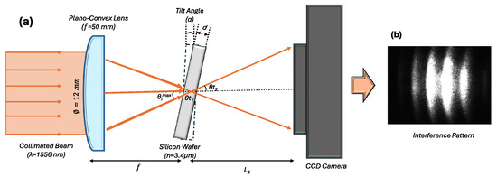
The experimental setup scheme implemented in this work is shown in Figure 1a. Here, the light emitted at 1550 nm by a DFB laser diode (Qphotonics QDFBLD-1550-5, Ann Arbor, MI, USA) was passed through a collimator with an output diameter of = 12 mm. Subsequently, the collimated beam was passed through the 50 mm focal length plano-convex lens (Thorlabs LA1433, Newton, NJ, USA). Later, its divergent beam illuminated a silicon wafer of thickness d = 800 m, which was double-side polished and has high parallelism (University Wafer, Boston, MA, USA). This wafer acted as an etalon, and it was mounted on a motorized continuous rotation stage. Furthermore, during the experiment, the Si wafer was kept at room temperature (25 °C) to avoid variations in its refractive index and thickness. After the wafer, the transmitted light strikes directly a CCD array (Point Gray CMLN-13S2M-CS, Richmond, BC, Canada), which has a resolution of 1296 × 966 pixels and an overall spatial dimension of 4.9 mm × 3.6 mm. Furthermore, the entire system was automated with LabVIEW software (National Instruments, Austin, TX, USA), allowing us to control the position wafer, acquire, and save images in a systematic way.
Figure 1.
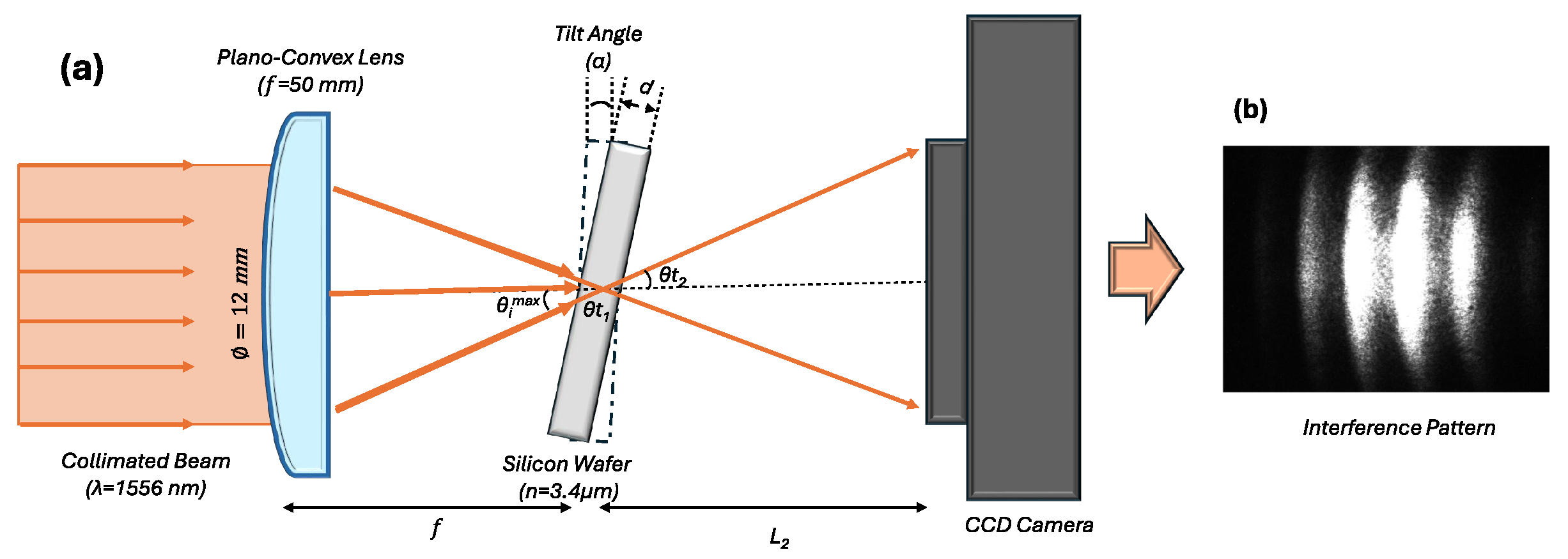
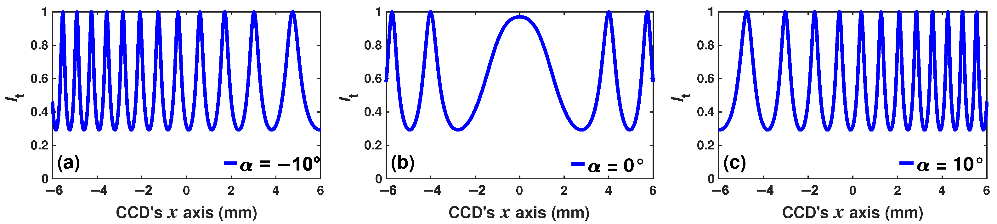
(a) Experimental setup for the wafer tilt angle measurement; (b) example of the image acquired for a fixed wafer angle.
In this setup, the etalon acts as a Fabry–Perot interferometer (FPI), which was precisely positioned on the axis and illuminated with a divergent beam. Therefore, a pattern of rings will be observed on the CCD screen [17]. Any change in either the optical thickness or the tilt angle of the FPI will induce a change in the transmitted intensity distribution pattern. Therefore, it is expected that the overall distribution pattern (interferogram) acquired with the CCD sensor will change as the wafer tilt angle is varied [18,19,20].
2.2. Simulated FPI Ring Pattern
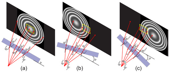
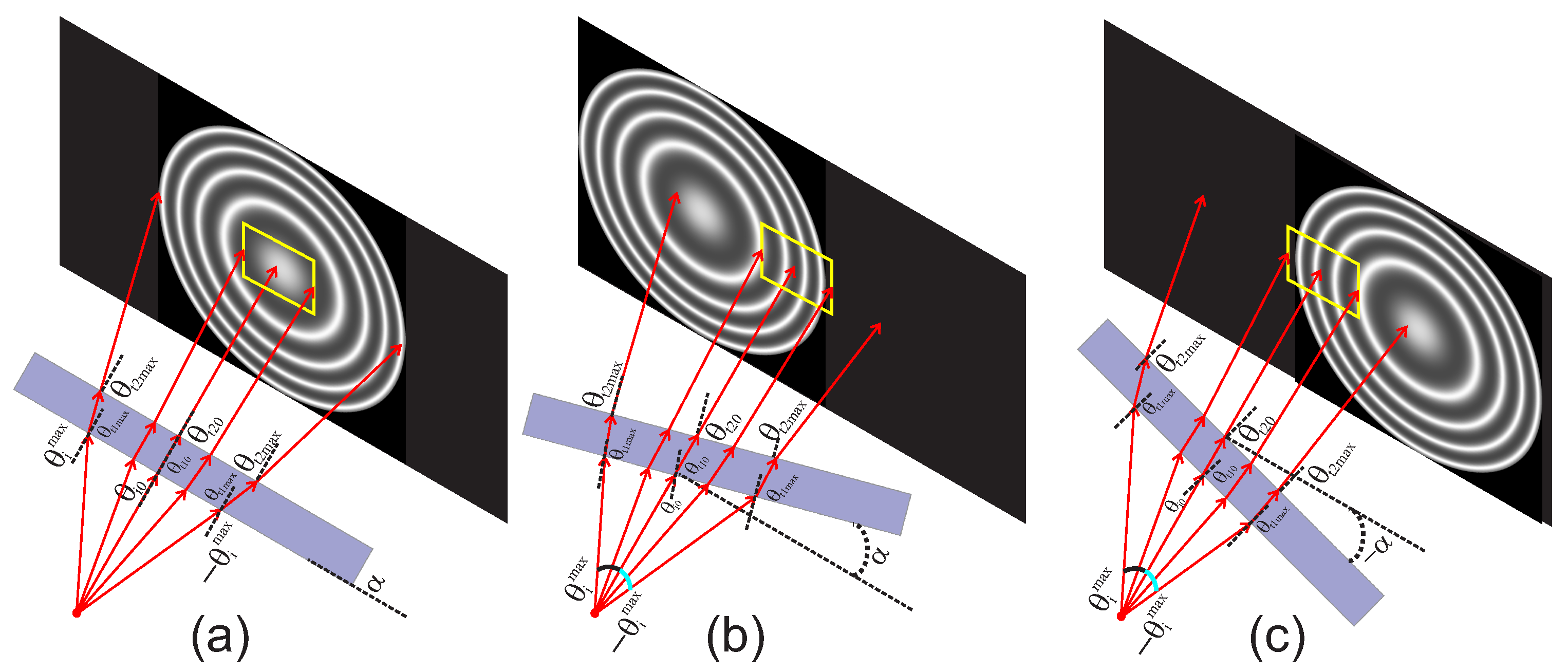
In the experimental setup (Figure 1) the Si wafer was illuminated with a cone of rays, which have different angles of incidence within the range ≤ ≤ (Figure 1). Moreover, the wafer can be tilted, over one axis, from ≤≤, in such a way that when 0 the Si wafer is placed parallel to the plane of the lens and the CCD array. Furthermore, when the wafer was tilted degrees, the angles of incidence of the rays were modified, and these can be described as . Later, the angles of the rays transmitted into the Si wafer, of thickness d, will generate the multiple internal reflections within the solid cavity, and these are given as , where the refractive indices of air and silicon are and , respectively. Moreover, the beams that were transmitted from the wafer to the air have angles defined as . Finally, the intensity distribution will be given by the Airy function, which can be represented as:
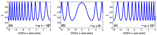
where . This intensity pattern will propagate from the wafer to the plane of the CCD array. The estimated spectra at the plane of view of the CCD for different tilt angles are presented in Figure 2. Moreover, as the CCD sensor remains fixed and has a limited area, only the part of the pattern will be detected.
Figure 2.
Relative transmitted intensity distribution at the plane of the CCD array when the tilt angle was (a) —10°, (b) 0° and (c) 10°.
In this arrangement, a spatial shift in the FPI ring pattern over the plane of observation of the CCD was induced as the wafer is tilted. In this way, the CCD sensor will detect rings segments as can be observed in Figure 3. For example, when the ring pattern will be centered in the CCD array and will capture only the central ring, as can be observed in Figure 3a. Here, it is important to mention that the area of the CCD is limited with a yellow rectangle in the figure. Moreover, when the Si wafer is tilted, the overall pattern of the rings is shifted and the CCD will capture just a few segments of the rings (Figure 3b,c).
Figure 3.
Ring pattern shifted over the CCD array as the tilt angle is fixed to (a) —10°, (b) 0° and (c) 10°.
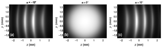
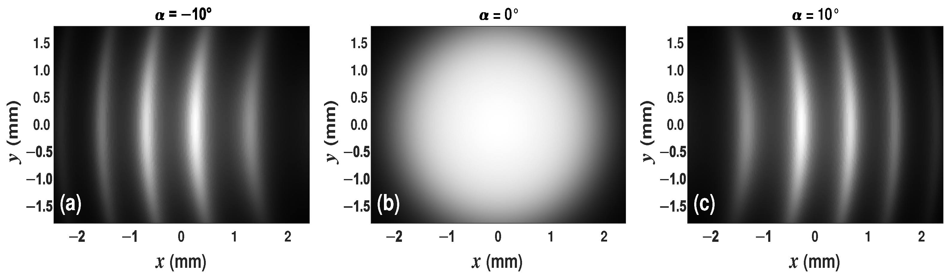
Finally, it is important to point out that, in order to take into consideration the beam profile of the DFB laser emission, the two-dimensional intensity distribution pattern must be multiplied by a Gaussian function. In Figure 4 are presented simulated images that will be provided by the CCD sensor for three different tilt angles.
Figure 4.
Simulated ring pattern segments observed by the CCD when the tilt angle of the Si wafer is (a) —10°, (b) 0° and (c) 10°.
2.3. Image Acquisition and Feature Extraction
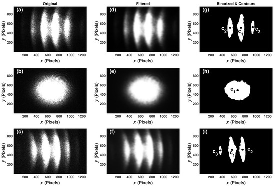
In order to characterize the operation of the optical sensing arrangement, a set of ring patterns (interferograms) was acquired for different angles of the wafer. Later, these were analyzed to extract some of their features to implement a machine learning regression capable of estimating the angle of the wafer from just one image. For each tilt angle at which the wafer was positioned, three images (interferograms) were acquired. In this way, 1071 images were captured, corresponding to 357 angular positions of the wafer, between —10.013° and 10.013° with steps of 0.056°, and their three corresponding replicas, labeled here as , and , respectively. As an example of the recorded images, in Figure 5a–c are shown the original raw interferograms acquired at —10.013°, 0° and 10.013°, respectively. In these images, it can be clearly seen that interferogram fringes were shifted as the Si wafer was tilted, as expected by the simulations. Also, it can be observed that the brightness and area of the fringes changed with the angle of incidence.
Figure 5.
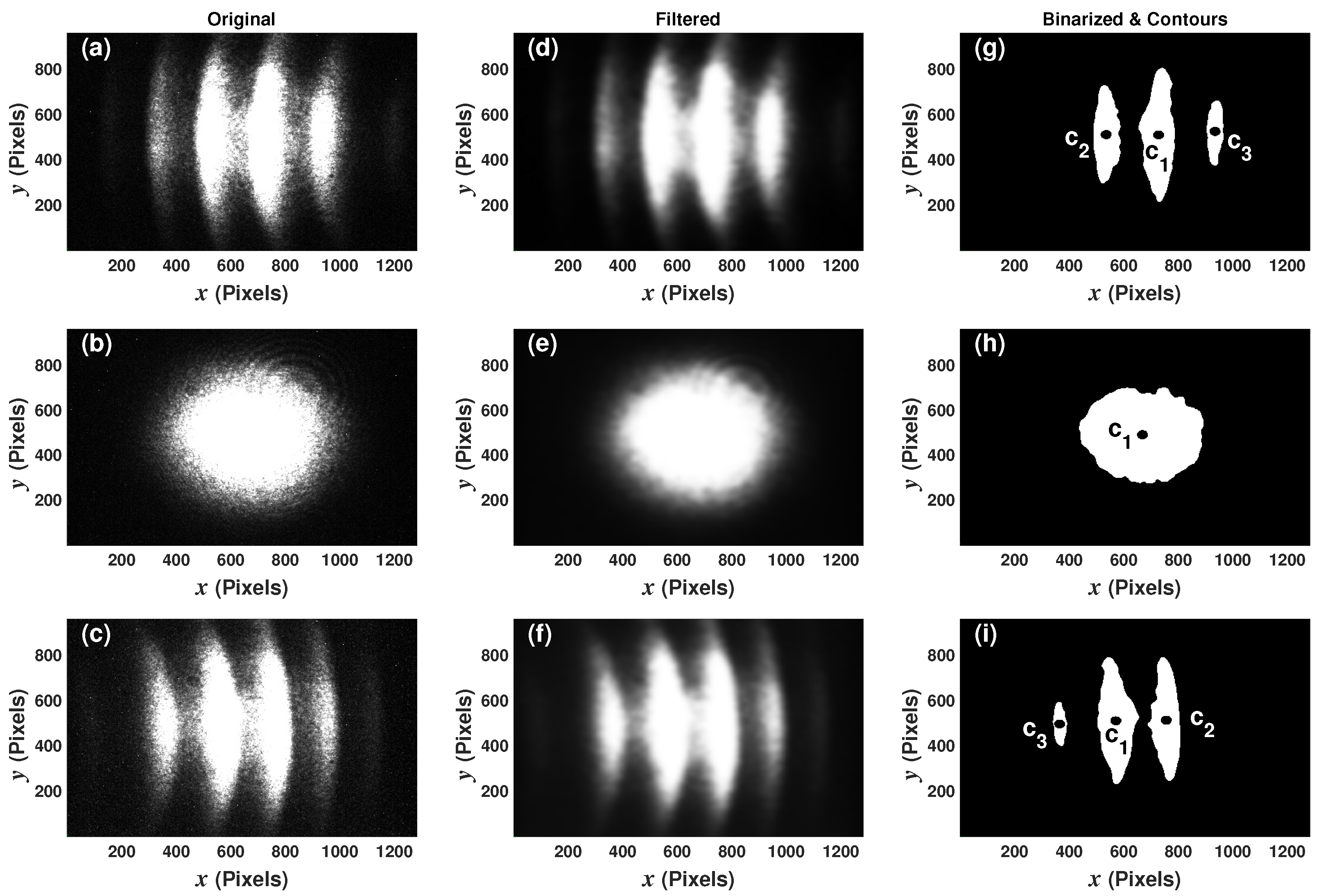
(a–c) Measured transmitted intensity distribution patterns; (d–f) low-pass filtered patterns; (g–i) detected objects in the acquired patterns at —10.013°, 0° and 10.013°, respectively.
2.4. Image Pre-Processing and Feature Extraction
The image pre-processing stage consisted of two steps. In the first one, images were filtered with a Gaussian low-pass filter for smoothing them and minimizing the high-frequency noise. In Figure 5d–f the filtered interferogram images are shown, which were acquired at —10.013°, 0° and 10.013°, respectively. In the second pre-processing stage step, images were binarized to highlight their most prominent objects. As an example, in Figure 5g–i the images obtained after the binarization step corresponding to the tilt angles of —10.013°, 0° and 10.013° are shown. Here, it was established that pixels with intensities larger than or equal to the threshold level of 220 in the filtered images must map as pixels with intensity of 255 (white) in the binarized images; otherwise, they must map as pixels with intensity 0 (black). The definition of the threshold level for the binarization procedure is important, since with a low level a few large objects can be found; as an example in Figure 6a shows the result of using a threshold level of 20. With higher levels the detected objects usually have a more detailed shape (Figure 6b); however, if the threshold is quite large, near 255, the detected object can be very small (Figure 6d) and even none can be identified. For this work, with a threshold level of 220, the detection of the most relevant segments of the rings presented in the interferogram was achieved (Figure 6c).
Figure 6.
Objects detected after the binarization procedure with threshold levels of (a) 20, (b) 150, (c) 220 and (d) 254.
The contours of all the localized objects in each image were then traced. In this case, the objects are the segments of the rings of the intensity distribution patterns. Finally, from these objects, the following features were extracted: the area of the region delimited by the contour (), the and coordinates of its centroid (ci) and its first-order moments of inertia and over the horizontal and vertical axes, respectively. Here, 1 corresponds to the largest object, while corresponds to the second larger object. For example, the centroids of the two largest objects detected in the images, acquired at —10.013°, 0°, and 10.013°, are shown in Figure 5g–i, respectively.
2.5. Interferogram Features and Dataset
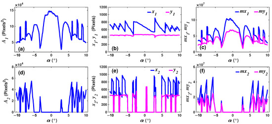
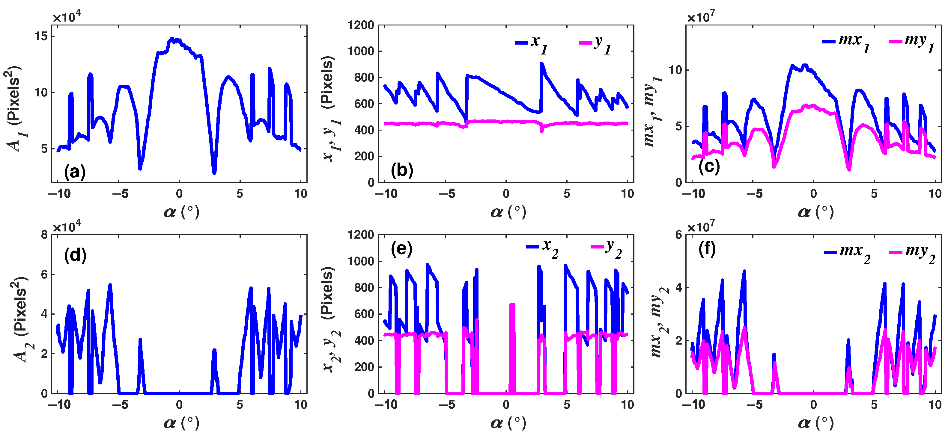
An experimental dataset (ED) was built with the extracted features of the three largest contours. In that way, each record (row) of the dataset has the predictors variables [] and the independent variable [] which is the angle at which the interferogram was acquired. Moreover, all predictor variables (X) have a nonlinear relationship with the tilt angle of the wafer , as can be observed in Figure 7 where the behavior of the features of the two largest objects (fringes) located in each interferogram are presented. For example, the coordinates and of the centroids c1 as a function of the angle are shown in Figure 7b. Similarly, the area of the largest object and the moments of inertia and are presented in Figure 7a and Figure 7c, respectively. The same features but corresponding to the second largest object are shown in Figure 7d–f.
Figure 7.
Relationship between the features (a,d) area (); (b,e) centroid coordinates (, ); (c,f) moment of inertia (, ) of the first () and second () largest objects detected in the captured interferograms as a function of the wafer’s tilt angle.
In addition, in these figures it can be observed that all features and the tilt angles have strong nonlinear relationships. Additionally, it can be seen that, for multiple wafer tilt angles, the same features were obtained, such as the centroid coordinates or (Figure 7b), which implies the presence of ambiguities. Moreover, the centroid coordinates of the second larger object presented a larger number of ambiguities and discontinuities (Figure 7e) within the same range of angles. Here, traditional methods such as linear regression or polynomial fits are not suitable to determine the tilt angle over the full range from —10.013° to 10.013°. Machine learning algorithms, such as artificial neural networks [21], can be an option to establish relationships between predictor variables (features) and tilt angle.
2.6. Training and Testing Datasets
The training dataset () was formed by randomly selecting 80% of the observations of each experimental replica , , and . The other 20% of the observations were used to build the testing dataset (). In this way, the training dataset has a size of 815 registers × 13 variables, while the testing dataset has a size of 215 registers × 13 variables.
3. Results
Due to ambiguities and the overall nonlinear behavior of extracted features, it can be quite difficult to determine the wafer tilt angle over a relatively wide measurement range by using traditional methods, such as multiple linear or polynomial regressions. Therefore, to overcome these issues, machine learning models can be used. Here, in particular, a regression based on an ensemble of artificial neural networks (ANNs) was implemented to estimate the tilt angle of the Si wafer considering the values of the extracted features of an interferogram.
3.1. Ensemble of ANNs
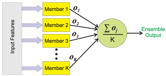
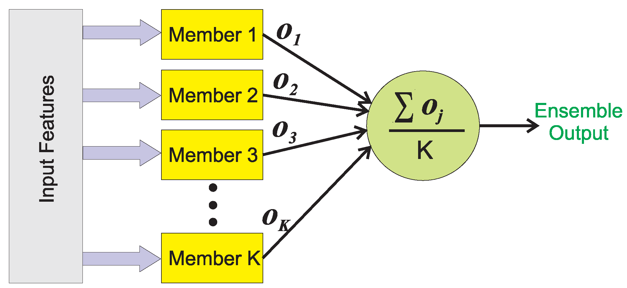
A regression can be implemented using an ensemble [22,23], that is a machine learning technique. Its main goal is to build a strong model by combining the output of multiple weak models [24]. This is important because in ANNs generally the models obtained after training will be different if this procedure is initialized with random weights. Therefore, each trained (weak) model will provide a different estimation of the output variable when the same feature values are presented as input. Here, an ensemble will take into account all different estimations of the weak models to generate a more robust overall output. There are different ways to implement an ensemble, for a regression, one of the simplest architecture consists in averaging the output of all weak members. The block diagram that represents this procedure is shown in Figure 8.
Figure 8.
Block diagram of an ensemble model for a regression.
3.2. Architecture of the Implemented ANNs
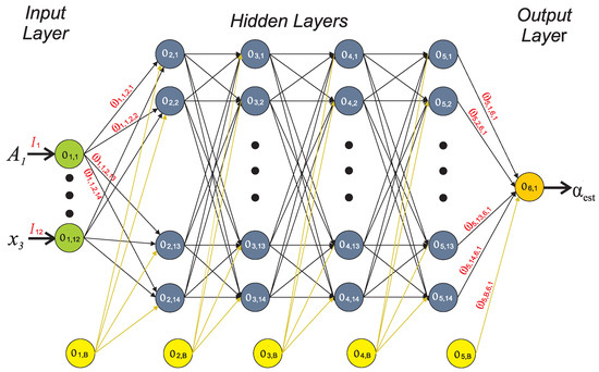
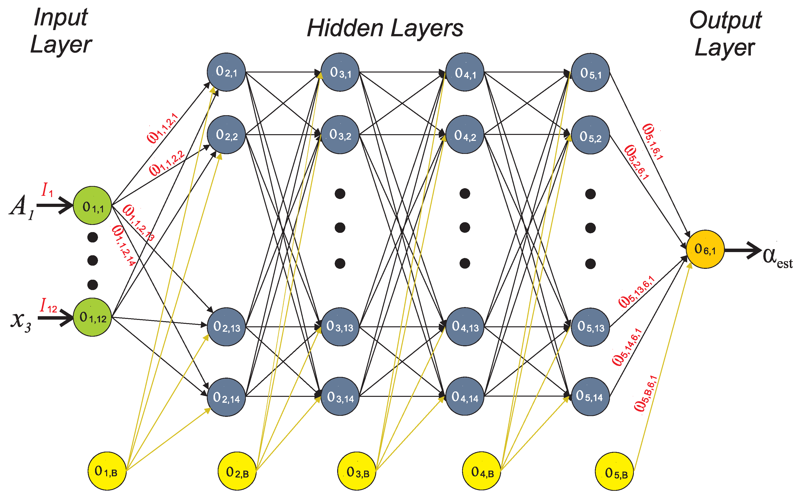
For this work, the weak members of the ensemble were five trained ANN models, which were all given the same input features values. In addition, the same ANN architecture was used for the five members. The architecture consisted of a network with one input and four hidden layers and one output layer. Moreover, the input layer has 12 neurons (denoted by green circles in Figure 9), one for each predictor (feature) variable. All hidden layers have 14 neurons (gray circles in Figure 9), while the output layer has one neuron that provides the estimated tilt angle (orange circle in Figure 9). Furthermore, for all neurons of hidden layers, a tangent hyperbolic (tanh) was used as activation function. Here, it is important to point out that, the output the k-th neuron of layer number l is denoted as (Figure 9). Moreover, for our ANN model, the neuron outputs of hidden layers can be expressed as [22]:
where tanh is the activation function of the neurons, is the weight of the linking connection between the output of the neuron () and the input of the neuron (), and M is the number of neurons in layer i. In the ANN model, a bias neuron () is aggregated in each layer, excepting in the output layer (yellow circles in Figure 9). Furthermore, for the input and the output layers the linear activation function was considered. Therefore, the outputs of the neurons of the input layer are given by:
where are the values of the features that feed the ANN model (Figure 9). Similarly, the result of the neuron of the output layer, that is the estimated tilt angle, can be written as:
Figure 9.
Architecture of the ANN models used for all members of the ensemble.
3.3. Performance of the Ensemble of ANNs
In this case, each ANN was trained with the same conditions: 10,000 epochs and Adam optimizer with learning rate of 0.0010. Moreover, the training of each model was initialized with random weight values, which induces that all members of the ensemble will have different performances, producing different estimated outputs [22]. Here, each ANN model was trained using the same training dataset, which has 856 registers (observations). Once the models were trained, the 215 observations contained in the testing dataset were presented to estimate the total output of the ensemble. Here, it is important to mention that the data from the testing dataset was not considered in the training procedure.
In addition, to estimate the performance of the implemented regression, two error metrics were evaluated, the mean absolute error (MAE) and the root mean squared error (RMSE), which are defined as:
and
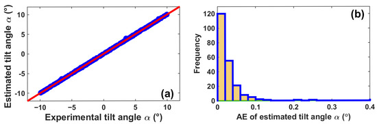
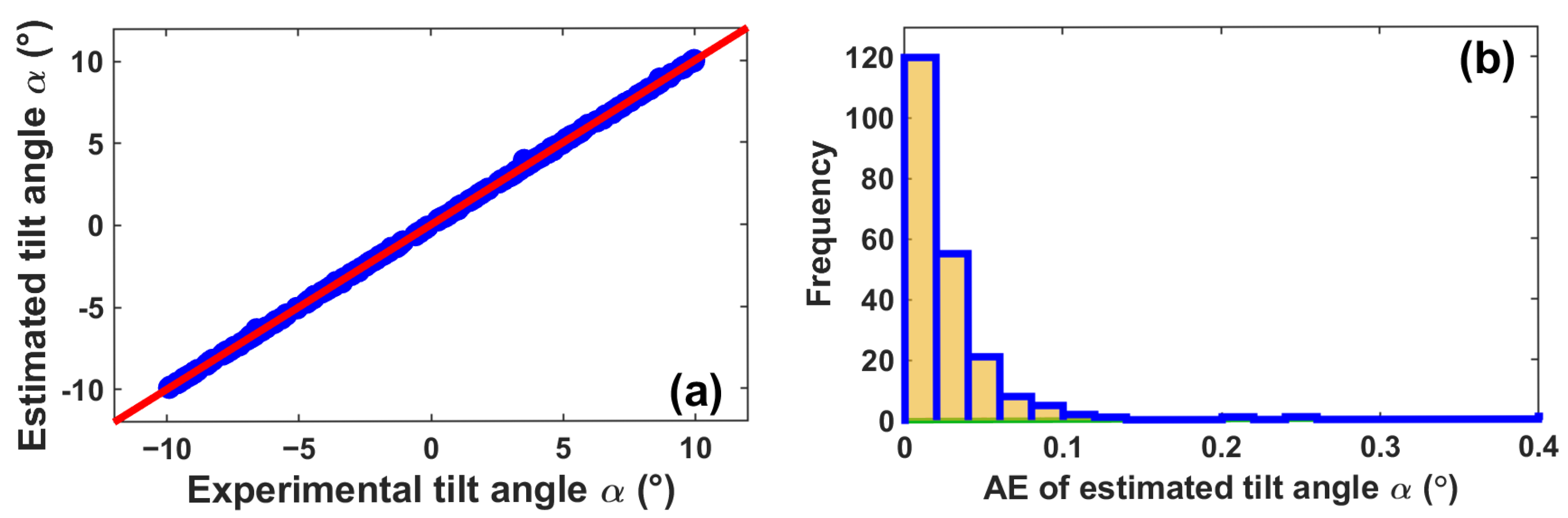
A comparison between the estimated tilt angles, provided by the ensemble, and the real angles is presented in Figure 10a, where it can be observed that the regression fits very well for all samples. It must be pointed out that in an perfect regression fit this comparison will generate a 45-degree straight line (red line). Here, it can be seen that practically all estimated angles form the straight line when compared with the real tilt angles (blue circles). Moreover, the distribution frequency of the absolute errors (AEs) between the estimated and real tilt angle values is shown in Figure 10b, where it can be observed that, for 175 cases, which represent the 81.39% observations of the test dataset, the AE is lower than 0.04°, and just a few cases presented errors larger than 0.2°, showing that the regression model generalizes very well in the measurement range from —10.013° to 10.013°. Furthermore, it was concluded that the tilt angle can be estimated with an MAE of 0.028° and an RMSE of 0.047°.
Figure 10.
(a) Comparison between estimated outputs of the ensemble () and the experimental tilt angles () and (b) their corresponding absolute error (AE) frequency distribution.
4. Discussion
In this work, it was demonstrated that the tilt angle of an optical etalon can be determined from a single-intensity distribution pattern (image) by applying machine learning algorithms. Moreover, an additional advantage of the proposal is that these results were achieved using a very simple optical experimental setup. Here, it should be pointed out that, in the optical arrangement, one of the most important sources of noise is the CCD itself. Practically all acquired images were quite noisy. However, this was minimized with the pre-processing stage, where images are low-pass filtered and the high-frequency noise was attenuated. Moreover, as the angle estimation depends on the position of the centroids, the high-frequency noise does not induce considerable negative effects. This represents an advantage and gives strength to the overall system. Furthermore, the ANN ensemble also contributes to minimization of the variability induced by the noise. Finally, in future work, the viability of using a similar ensemble to estimate the angles of the wafer when it is inclined over two axes.
5. Conclusions
It was shown that the tilt angle can be determined by means of an ensemble of ANN regression by extracting some features of a single interferogram. These features are used as inputs of the ANN models. Here, the extracted features were the area, the coordinates of the centroid, and the first-order moment of inertia of the largest fringes localized in the images. Furthermore, these features present a strong nonlinear relationship with the Si wafer tilt angle, with several discontinuities and ambiguities in a relatively short angle range. This nonlinear behavior was overcome by means of an ensemble of artificial neural networks that was able to estimate the tilt angle between the measurement range of —10.013° to 10.013°, with a mean absolute error of 0.028° and a mean squared error of 0.047°. This overall performance shows that by using this methodology the tilt angle can be estimated with high precision and also the direction of the tilt angle by taking just one image.
Author Contributions
Conceptualization, J.C.M.-C., E.V.-R. and A.D.G.-C.; methodology, J.C.M.-C. and R.G.-C.; software, J.C.M.-C., S.I.R.-Z. and R.G.-C.; formal analysis, J.C.M.-C., E.V.-R. and R.G.-C.; investigation, A.D.G.-C. and R.G.-C.; data curation, A.D.G.-C., J.J.P.-M. and S.I.R.-Z.; writing—original draft preparation, J.C.M.-C. and E.V.-R.; writing—review and editing, R.G.-C., A.D.G.-C., S.I.R.-Z. and J.J.P.-M.; funding acquisition, E.V.-R. and A.D.G.-C. All authors have read and agreed to the published version of the manuscript.
Funding
J.C. Morales-Castro is grateful to the Secretaría de Ciencia, Humanidades, Tecnología e Innovación de México (SECIHTI), for the provided student research grant under number 1104964.
Institutional Review Board Statement
Not applicable.
Informed Consent Statement
Not applicable.
Data Availability Statement
The raw data supporting the conclusions of this article are not readily available because they are part of an ongoing study but will be made available by the authors upon request.
Conflicts of Interest
The authors declare no conflicts of interest.
References
- Bajić, J.S.; Stupar, D.Z.; Manojlović, L.M.; Slankamenac, M.P.; Živanov, M.B. A simple, low-cost, high-sensitivity fiber-optic tilt sensor. Sens. Actuators A Phys. 2012, 185, 33–38. [Google Scholar] [CrossRef] [Scilit]
- Osuch, T.; Markowski, K.; Manujło, A.; Jędrzejewski, K. Coupling independent fiber optic tilt and temperature sensor based on chirped tapered fiber Bragg grating in double-pass configuration. Sens. Actuators A Phys. 2016, 252, 76–81. [Google Scholar] [CrossRef] [Scilit]
- Mou, J.; Huang, T.; Shu, X. Theory and error compensation method based on the tilt sensor adopted in dynamic angle measurement of the fiber optic gyroscope. Opt. Fiber Technol. 2020, 60, 102368. [Google Scholar] [CrossRef] [Scilit]
- Mandal, L.; Ganesan, A.R. Tilt measurement using multiple reflections Michelson interferometer and single interferogram. Optik 2025, 321, 172187. [Google Scholar] [CrossRef] [Scilit]
- Malacara, D.; Harris, O. Interferometric Measurement of Angles. Appl. Opt. 1970, 9, 1630–1633. [Google Scholar] [CrossRef] [Scilit] [PubMed]
- Pretheesh Kumar, V.C.; Charles, J.; Angarai, G.; Umapathy, S. Increasing the sensitivity for tilt measurement using a cyclic interferometer with multiple reflections. Opt. Eng. 2016, 55, 084103. [Google Scholar] [CrossRef] [Scilit]
- Zhong, Z.W.; Zhao, L.P.; Lin, H.H. Development and investigation of an optical tilt sensor. Opt. Commun. 2006, 261, 23–28. [Google Scholar] [CrossRef] [Scilit]
- Chen, Y.; Yu, Y.; Xu, Y.; Wang, Z.; Li, N.; Xu, W.; Zhang, Z. Seawater Dual Parametric Fiber Optic Temperature and Pressure Sensors Demodulated by Machine Learning Method. J. Phys. Conf. Ser. 2024, 2718, 012049. [Google Scholar] [CrossRef] [Scilit]
- Michelucci, U.; Baumgartner, M.; Venturini, F. Optical Oxygen Sensing with Artificial Intelligence. Sensors 2019, 19, 777. [Google Scholar] [CrossRef] [Scilit] [PubMed]
- Noor, M.Y.M.; Azizan, A.; Saimon, S.M.; Azmi, A.I.; Iqbal, F.; Abdullah, A.S.; Zhang, J.; Shapiai, M.I. Decision Tree Regression Supervised Machine Learning Assisted Large Dynamic Range Refractive Index Detection Using MMI Coreless Multimode Fiber Sensor. IEEE Sens. J. 2024, 24, 12433–12440. [Google Scholar] [CrossRef] [Scilit]
- Paniagua-Medina, J.J.; Vargas-Rodriguez, E.; Guzman-Chavez, A.D.; Morales-Castro, J.C.; Correa-Jurado, R.J. Random Forest Regression for Improving the Measurement Range of a Temperature Interferometric Sensor. IEEE Photon. Technol. Lett. 2025, 37, 101–104. [Google Scholar] [CrossRef] [Scilit]
- Guzman-Chavez, A.D.; Vargas-Rodriguez, E.; Vargas-Rodriguez, B.L.; Garcia-Ramirez, M.A. Viability of Artificial Neural Networks for Widen the Measurement Range of Interferometric Sensors. IEEE Photon. Technol. Lett. 2022, 34, 915–918. [Google Scholar] [CrossRef] [Scilit]
- Guzman-Chavez, A.D.; Vargas-Rodriguez, E. The Application of Kernel Ridge Regression for the Improvement of a Sensing Interferometric System. Sensors 2025, 25, 1292. [Google Scholar] [CrossRef] [Scilit] [PubMed]
- Cao, J.; Wang, X.; Huang, B.; Lou, S.; Chu, P.K.; Sheng, Z. Using machine learning to enlarge the measurement range and promote the compactness of the optical fiber torsion sensor based on the Sagnac interferometer. Opt. Express 2024, 32, 6929–6944. [Google Scholar] [CrossRef] [Scilit] [PubMed]
- Martinez-Manuel, R.; Valentin-Coronado, L.M.; Esquivel-Hernandez, J.; Monga, K.J.J.; La Rochelle, S. Machine learning implementation for unambiguous refractive index measurement using a self-referenced fiber refractometer. IEEE Sens. J. 2022, 22, 14134–14141. [Google Scholar] [CrossRef] [Scilit]
- Valentín-Coronado, L.M.; Martínez-Manuel, R.; Esquivel-Hernández, J.; Martínez-Guerrero, M.d.l.A.; LaRochelle, S. Bending classification from interference signals of a fiber optic sensor using shallow learning and convolutional neural networks. Pattern Recognit. Lett. 2024, 186, 354–360. [Google Scholar] [CrossRef] [Scilit]
- Vaughan, J.M. The Fabry-Perot Interferometer History, Theory, Practice and Applications; Adam Hilger: Bristol, UK, 1989. [Google Scholar] [CrossRef] [Scilit]
- Nakamura, K.; Kurosawa, Y.; Ishikawa, K. Tunable optical filters using a LiNbO3 torsional actuator with a Fabry–Perot etalon. Appl. Phys. Lett. 1996, 68, 2799–2800. [Google Scholar] [CrossRef] [Scilit]
- Lin, L.Y.; Shen, J.L.; Lee, S.S.; Wu, M.C.; Sergent, A.M. Tunable three-dimensional solid Fabry-Perot etalons fabricated by surface-micromachining. IEEE Photonics Technol. Lett. 1996, 8, 101–103. [Google Scholar] [CrossRef] [Scilit]
- Peterson, D.G.; Yariv, A. Interferometry and Laser Control with Solid Fabry–Perot Etalons. Appl. Opt. 1966, 5, 985–991. [Google Scholar] [CrossRef] [Scilit] [PubMed]
- Zavala-Guzmán, A.; Vargas-Rodriguez, E.; Guzman-Chavez, A.D.; Raja Ibrahim, R.K.; García-Ramírez, M.A. Artificial neural networks to control the wavelength and peak intensity of a DFB laser diode emission. Laser Phys. Lett. 2025, 22, 116203. [Google Scholar] [CrossRef] [Scilit]
- Heaton, J. Applications of Deep Neural Networks; Cornell University: Ithaca, NY, USA, 2020. [Google Scholar] [CrossRef] [Scilit]
- Nixon, J.; Lakshminarayanan, B.; Tran, D. Why Are Bootstrapped Deep Ensembles Not Better? In Proceedings of the ”1st I Can’t Believe It’s Not Better! Workshop (ICBINB @ NeurIPS 2020)”; Neural Information Processing Systems: Vancouver, BC, Canada, 2020. [Google Scholar]
- Jo, T. Machine Learning Foundations Supervised, Unsupervised, and Advanced Learning; Springer International Publishing: Berlin/Heidelberg, Germany, 2021. [Google Scholar] [CrossRef] [Scilit]


Disclaimer/Publisher’s Note: The statements, opinions and data contained in all publications are solely those of the individual author(s) and contributor(s) and not of MDPI and/or the editor(s). MDPI and/or the editor(s) disclaim responsibility for any injury to people or property resulting from any ideas, methods, instructions or products referred to in the content. |
© 2026 by the authors. Licensee MDPI, Basel, Switzerland. This article is an open access article distributed under the terms and conditions of the Creative Commons Attribution (CC BY) license.