Vector Vortices in Linear Optical Media

Abstract

The present work investigates the linear regime of propagation of modulated vector optical fields in isotropic dispersive media by focusing on the formation of complex vector vortex structures with amplitude-type singularities. A mathematical algorithm designed to derive novel exact analytical solutions for the linear vector amplitude equation is presented, enabling the systematic development and classification of diffraction-free vector solutions. Various types of solutions for the two orthogonal components of the vector amplitude function are obtained, resulting in non-trivial spatial amplitude structures in their cross sections. The proposed approach allows for precise analytical governance of the spatial and polarization properties of the obtained vortices via the vortex parameter n. The presented model offers a comprehensive framework for generating different types of vector vortex structures by choosing the values of the parameters n and m, depending on the initial phase of the components. The derived solutions extend the capabilities of conventional phase modulation techniques. It is demonstrated that by changing the vortex parameter n, the structural complexity of both the amplitude distributions and polarization patterns increases. A number of numerical simulations, based on the obtained analytical solutions, are performed. They validate the model and clearly illustrate the characteristic vectorial features via detailed vector diagrams.

1. Introduction

Modern singular optics is one of the fastest growing areas of contemporary photonics. Optical vortices can generally be divided into two main classes: phase vortices and polarization vortices. Phase vortices originate from singularities in the phase distribution of the optical field and have been extensively investigated, both theoretically and experimentally [1,2,3]. Their generation is relatively well understood, and their characteristic features such as the helical phase front and orbital angular momentum (OAM) have been widely demonstrated in laboratory conditions. These vortices are typically described by scalar beam models, such as Laguerre–Gaussian or Bessel beams, and exhibit phase dislocations. The topological charge of the vortex determines the number of $2\pi$ phase windings around the singularity and directly relates to the amount of OAM carried by the beam [4,5,6,7]. Ultra-short femtosecond laser pulses have proven especially effective in generating phase vortices, due to their broad spectral content and strong spatial-temporal localization [8]. By employing spatial light modulators, spiral phase plates, or nonlinear processes in anisotropic media, it is possible to imprint vortex phase structures onto femtosecond pulses with high precision [8,9]. The phase optical vortices have been extensively studied for their fundamental properties and their broad range of applications in optical trapping, high-resolution microscopy, and optical communications [10,11].

In contrast, the polarization vortices are not associated with helical phase structures or orbital angular momentum. Instead, they arise in the vector components of an optical field, exhibiting singularities in the amplitude distribution. These vortices are formed by two linearly polarized components, one along the axis x and the other along y, each of which has a vortex in its intensity field. A feature of this type of optical structure is that the superposition of the two linearly polarized components leads to their disappearance in the total intensity field. The solutions for the components of the amplitude function have a characteristic singularity at zero in the vortex. The polarization vortices cannot be directly observed in the total field but become visible only when one field component is selectively filtered (e.g., suppressing the $A_y$ component reveals the structure in $A_x$).

By optical vortices with amplitude-type singularity, we understand the well-known polarization vortices in the literature. In the linear regime of propagation, they do not differ significantly from phase vortices. In the nonlinear case, polarization vortex structures exist as solutions for the components of the vector amplitude function [12,13,14,15].

The generation of amplitude singularities poses significant experimental challenges. For this reason, in recent decades, the study of laser vortex structures with amplitude-type singularity has become important [16,17,18,19,20]. Polarization vortices are particularly relevant in the context of ultra-short laser pulse propagation, where the vectorial and dispersive properties of the medium become significant [12,13]. Optical fibers with a step-index profile, due to their simple geometry and well-understood modal structure, provide a convenient and widely used platform to study such phenomena [13].

Our current work focuses on the theoretical description and numerical investigation of vector vortex structures in media with a linear optical response. The linear regime of propagation of modulated optical waves in isotropic dispersive media is studied, taking into account the conditions under which the polarization vortices can be generated. By employing the vector linear amplitude equation, new exact analytical diffraction-free vector solutions that describe amplitude singularities in the components of the optical wave are derived. An important feature is the construction of vector diagrams that describe the local rotation of the electric field vector. These diagrams not only illustrate the underlying vector vortex structure but also serve as a confirmation of the formation of polarization vortices. The arrows in the vector diagrams indicate the polarization direction of the optical field. Their length is proportional to the magnitude of the electric field intensity vector. The vectors are referenced to their starting point.

With regard to the Laguerre–Gaussian beams with opposite topological charges or Hermite–Gaussian beams with orthogonal linear polarization, our newly obtained type of solution is conceptually closer to the second one, i.e., to beams with orthogonal linear polarization, and yet it represents a fundamentally different class of solution.

The obtained analytical solutions contribute to the theoretical foundation of singular optics in isotropic media and open new avenues for manipulating the spatial structure of laser light in optical systems. The polarization vortices are of particular interest because they expand the concept of structured light beyond the well-studied phase singularities, offering novel perspectives for fundamental studies and potential applications. The unique properties of these vortex structures are expected to play an important role in the next generation of photonic technologies, particularly in the areas of ultrafast signal processing, information encoding and encryption, polarization-sensitive sensing, the design of structured laser sources, and light–matter interaction in structured media.

2. Finding an Exact Analytical Solution to the Linear Amplitude Equation

2.1. Basic Equations

The vector linear amplitude equation in the local time coordinate system, describing the propagation of modulated optical waves in isotropic dispersive media, is of the kind [21,22]:

$$\begin{array}{c}\hfill 2i\alpha {\delta }^2{\displaystyle \frac{\partial \overrightarrow{\check{A}}}{\partial \check{z}}}+{\Delta }_{\perp }\overrightarrow{\check{A}}+\beta {\delta }^2{\displaystyle \frac{{\partial }^2\overrightarrow{\check{A}}}{\partial {\check{t}}^2}}+{\delta }^2\left[{\displaystyle \frac{{\partial }^2\overrightarrow{\check{A}}}{\partial {\check{z}}^2}}-2{\displaystyle \frac{{\partial }^2\overrightarrow{\check{A}}}{\partial \check{t}\partial \check{z}}}\right]=0,\end{array}$$

(1)

where $\overrightarrow{\check{A}}$ is the vector amplitude function and ${\Delta }_{\perp }$ is the transverse Laplace operator. In the Equation (1) the constant $\alpha$ gives the number of oscillations of the electric field at level $1/e$ of the amplitude function’s maximum, $\beta$ is a parameter, connected with the second-order dispersion of the medium, and $\delta$ presents a relation between the transverse and longitudinal dimensions of the modulation wave. They can be presented as follows:

$$\begin{array}{c}\hfill \alpha =k_0{z}_0,z_0=v_{gr}{T}_0,\beta =k_0{v}_{gr}^2\mid k^{″}\mid ,\delta ={\displaystyle \frac{r_0}{z_0}},{\Delta }_{\perp }=\left({\displaystyle \frac{{\partial }^2}{\partial {\check{x}}^2}}+{\displaystyle \frac{{\partial }^2}{\partial {\check{y}}^2}}\right),\end{array}$$

(2)

where $k_0$ is the wave number, $k^{″}$ is the second derivative of the wave number (group velocity dispersion), $z_0$ and $r_0$ are respectively the initial longitudinal and transverse sizes of the modulated optical wave, $T_0$ is the initial time duration and $v_{gr}$ is the group velocity.

Here, it is important to mention that the vector amplitude function describes both localized optical waves (pulses) and amplitude-modulated waves. In the case of laser pulses, the characteristic spatial and temporal dimensions correspond to its transverse width and time duration, measured at the level of $1/e$ of the amplitude’s peak. When modulated optical waves are considered, the transverse spot size is defined analogously, while the longitudinal temporal modulation is determined at the $1/e$ level of the amplitude of the periodic wave.

It is assumed that the vector amplitude function has components: $\overrightarrow{\check{A}}=({\check{A}}_x,{\check{A}}_y,0)$. Equation (1) can be written in dimensionless form by using the following substitutions:

$$\begin{array}{c}\hfill \overrightarrow{\check{A}}=A_0\overrightarrow{A},\check{z}=z_{0}z,\check{x}=r_{0}x,\check{y}=r_{0}y,t={\displaystyle \frac{\check{t}-v_{gr}\check{z}}{T_0}}.\end{array}$$

(3)

We can present the main equation in a cylindrical coordinate system by applying the following substitutions:

$$\begin{array}{c}\hfill x=rcos\theta ,y=rsin\theta ,x^2+y^2=r^2,\theta =arctg{\displaystyle \frac{y}{x}},\\ \hfill {\Delta }_{\perp }={\displaystyle \frac{{\partial }^2}{\partial x^2}}+{\displaystyle \frac{{\partial }^2}{\partial y^2}}={\displaystyle \frac{{\partial }^2}{\partial r^2}}+{\displaystyle \frac{1}{r}}{\displaystyle \frac{\partial }{\partial r}}+{\displaystyle \frac{1}{r^2}}{\displaystyle \frac{{\partial }^2}{\partial {\theta }^2}}.\end{array}$$

(4)

Thus, Equation (1) takes the following scalar dimensionless forms for each component of the modulated optical wave:

$$\begin{array}{c}\hfill 2i\alpha {\delta }^2{\displaystyle \frac{\partial A_x}{\partial z}}+\beta {\delta }^2{\displaystyle \frac{{\partial }^2{A}_x}{\partial t^2}}+{\delta }^2\left[{\displaystyle \frac{{\partial }^2{A}_x}{\partial z^2}}-2{\displaystyle \frac{{\partial }^2{A}_x}{\partial t\partial z}}\right]+\left[{\displaystyle \frac{{\partial }^2{A}_x}{\partial r^2}}+{\displaystyle \frac{1}{r}}{\displaystyle \frac{\partial A_x}{\partial r}}+{\displaystyle \frac{1}{r^2}}{\displaystyle \frac{{\partial }^2{A}_x}{\partial {\theta }^2}}\right]=0,\end{array}$$

(5)

$$\begin{array}{c}\hfill 2i\alpha {\delta }^2{\displaystyle \frac{\partial A_y}{\partial z}}+\beta {\delta }^2{\displaystyle \frac{{\partial }^2{A}_y}{\partial t^2}}+{\delta }^2\left[{\displaystyle \frac{{\partial }^2{A}_y}{\partial z^2}}-2{\displaystyle \frac{{\partial }^2{A}_y}{\partial t\partial z}}\right]+\left[{\displaystyle \frac{{\partial }^2{A}_y}{\partial r^2}}+{\displaystyle \frac{1}{r}}{\displaystyle \frac{\partial A_y}{\partial r}}+{\displaystyle \frac{1}{r^2}}{\displaystyle \frac{{\partial }^2{A}_y}{\partial {\theta }^2}}\right]=0.\end{array}$$

(6)

2.2. Finding Exact Analytical Solutions for the Components of the Amplitude Function

The system above contains two linear partial differential equations of second order with four variables ($r,\theta ,z$ and t). In order to find a solution of that system, we will use the method of separation of variables and search for diffraction-free solutions, for which the transverse profile of the modulation wave does not depend on z. For this purpose, the following assumptions are made: [23,24]

$$\begin{array}{c}\hfill A_x(r,\theta ,z,t)=V_x(z,t)P_x(r,\theta ),\end{array}$$

(7)

$$\begin{array}{c}\hfill A_y(r,\theta ,z,t)=V_y(z,t)P_y(r,\theta ).\end{array}$$

(8)

Only for this limited class of assumptions is it possible to obtain diffraction-free solutions that describe amplitude-type vortex structures in the field components. After a few simplifications, the following equations are obtained:

$$\begin{array}{c}\hfill \left[2i\alpha {\delta }^2{\displaystyle \frac{\partial V_x}{\partial z}}+\beta {\delta }^2{\displaystyle \frac{{\partial }^2{V}_x}{\partial t^2}}+{\delta }^2\left({\displaystyle \frac{{\partial }^2{V}_x}{\partial z^2}}-2{\displaystyle \frac{{\partial }^2{V}_x}{\partial t\partial z}}\right)\right]{\displaystyle \frac{1}{V_x}}+\\ \hfill \left[{\displaystyle \frac{{\partial }^2{P}_x}{\partial r^2}}+{\displaystyle \frac{1}{r}}{\displaystyle \frac{\partial P_x}{\partial r}}+{\displaystyle \frac{1}{r^2}}{\displaystyle \frac{{\partial }^2{P}_x}{\partial {\theta }^2}}\right]{\displaystyle \frac{1}{P_x}}=0.\end{array}$$

(9)

$$\begin{array}{c}\hfill \left[2i\alpha {\delta }^2{\displaystyle \frac{\partial V_y}{\partial z}}+\beta {\delta }^2{\displaystyle \frac{{\partial }^2{V}_y}{\partial t^2}}+{\delta }^2\left({\displaystyle \frac{{\partial }^2{V}_y}{\partial z^2}}-2{\displaystyle \frac{{\partial }^2{V}_y}{\partial t\partial z}}\right)\right]{\displaystyle \frac{1}{V_y}}+\\ \hfill \left[{\displaystyle \frac{{\partial }^2{P}_y}{\partial r^2}}+{\displaystyle \frac{1}{r}}{\displaystyle \frac{\partial P_y}{\partial r}}+{\displaystyle \frac{1}{r^2}}{\displaystyle \frac{{\partial }^2{P}_y}{\partial {\theta }^2}}\right]{\displaystyle \frac{1}{P_y}}=0.\end{array}$$

(10)

For the above equality to be fulfilled, both addends in the equation must be equal to the same constant, but with opposite sign. In this way, after several transformations, we derive the following system of equations:

$$\begin{array}{c}\hfill 2i\alpha {\displaystyle \frac{\partial V_x}{\partial z}}+\beta {\displaystyle \frac{{\partial }^2{V}_x}{\partial t^2}}+{\displaystyle \frac{{\partial }^2{V}_x}{\partial z^2}}-2{\displaystyle \frac{{\partial }^2{V}_x}{\partial t\partial z}}-{\displaystyle \frac{C}{{\delta }^2}}{V}_x=0,\end{array}$$

(11)

$$\begin{array}{c}\hfill {\displaystyle \frac{{\partial }^2{P}_x}{\partial r^2}}+{\displaystyle \frac{1}{r}}{\displaystyle \frac{\partial P_x}{\partial r}}+{\displaystyle \frac{1}{r^2}}{\displaystyle \frac{{\partial }^2{P}_x}{\partial {\theta }^2}}+C{P}_x=0,\end{array}$$

(12)

$$\begin{array}{c}\hfill 2i\alpha {\displaystyle \frac{\partial V_y}{\partial z}}+\beta {\displaystyle \frac{{\partial }^2{V}_y}{\partial t^2}}+{\displaystyle \frac{{\partial }^2{V}_y}{\partial z^2}}-2{\displaystyle \frac{{\partial }^2{V}_y}{\partial t\partial z}}-{\displaystyle \frac{C}{{\delta }^2}}{V}_y=0,\end{array}$$

(13)

$$\begin{array}{c}\hfill {\displaystyle \frac{{\partial }^2{P}_y}{\partial r^2}}+{\displaystyle \frac{1}{r}}{\displaystyle \frac{\partial P_y}{\partial r}}+{\displaystyle \frac{1}{r^2}}{\displaystyle \frac{{\partial }^2{P}_y}{\partial {\theta }^2}}+C{P}_y=0,\end{array}$$

(14)

where C is a separation constant [23,24].

The separation constant is introduced as a result of the mathematical model we utilize. Depending on whether C is equal to or different from zero, we obtain different classes of solutions, which carry distinct physical meanings.

2.2.1. Finding Exact Analytical Solutions for the Components of the Amplitude Function When $C\ne 0$

First, we will consider the case in which $C\ne 0$. We solve the equations above separately, starting with the expressions (12) and (14). Here, we will again use the method of separation of variables. Thus, the following substitutions are made:

$$\begin{array}{c}\hfill P_x(r,\theta )=f\left(r\right)cos(g\left(r\right)+n\theta ),\end{array}$$

(15)

$$\begin{array}{c}\hfill P_y(r,\theta )=f\left(r\right)sin(g\left(r\right)+n\theta ),\end{array}$$

(16)

where $n=const$. After a couple of transformations, we obtain the following equations:

$$\begin{array}{c}\hfill cos\left(g\right(r)+n\theta )\left[f^{″}-f{\left(g^{\prime }\right)}^2+{\displaystyle \frac{f^{\prime }}{r}}-{\displaystyle \frac{n^2}{r^2}}f+Cf\right]-\\ \hfill sin\left(g\right(r)+n\theta )\left[2f^{\prime }{g}^{\prime }+f{g}^{″}+{\displaystyle \frac{f{g}^{\prime }}{r}}\right]=0.\end{array}$$

(17)

$$\begin{array}{c}\hfill sin\left(g\right(r)+n\theta )\left[f^{″}-f{\left(g^{\prime }\right)}^2+{\displaystyle \frac{f^{\prime }}{r}}-{\displaystyle \frac{n^2}{r^2}}f+Cf\right]-\\ \hfill cos\left(g\right(r)+n\theta )\left[2f^{\prime }{g}^{\prime }+f{g}^{″}+{\displaystyle \frac{f{g}^{\prime }}{r}}\right]=0.\end{array}$$

(18)

In order for the equalities to be fulfilled, the expressions in brackets must be equal to zero. First, they are multiplied by functions $sin$ and $cos$. Thus, we obtain the following two differential equations for the two independent functions $f\left(r\right)$ and $g\left(r\right)$:

$$\begin{array}{c}\hfill f^{″}-f{\left(g^{\prime }\right)}^2+{\displaystyle \frac{f^{\prime }}{r}}-{\displaystyle \frac{n^2}{r^2}}f+Cf=0,\end{array}$$

(19)

$$\begin{array}{c}\hfill 2f^{\prime }{g}^{\prime }+f{g}^{″}+{\displaystyle \frac{f{g}^{\prime }}{r}}=0.\end{array}$$

(20)

Let us first consider Equation (20). We divide both sides by $\left(f{g}^{\prime }\right)$ and then integrate the obtained expression. After a couple of calculations, we find that

$$\begin{array}{c}\hfill f^{2}r{g}^{\prime }=B=const,\end{array}$$

(21)

where B is integration constant. From this expression we obtain a relation between the functions $f\left(r\right)$ and $g\left(r\right)$. To determine the two unknown functions, let us assume that

$$\begin{array}{c}\hfill g\left(r\right)=m{r}^{\mu },\end{array}$$

(22)

where m and $\mu$ are constants. We substitute expression (22) in Formula (21). Thus, we derive

$$\begin{array}{c}\hfill f=\sqrt{{\displaystyle \frac{B}{m\mu }}}{r}^{-{\displaystyle \frac{\mu }{2}}}.\end{array}$$

(23)

To determine $\mu$, we find the derivatives of the above expression and substitute them into Equation (17):

$$\begin{array}{c}\hfill r^{-{\displaystyle \frac{\mu }{2}}-2}\left({\displaystyle \frac{{\mu }^2}{4}}-n^2\right)-m^2{\mu }^2{r}^{2\mu -2-{\displaystyle \frac{\mu }{2}}}+C{r}^{-{\displaystyle \frac{\mu }{2}}}=0.\end{array}$$

(24)

In order for the equality to be fulfilled, the constants need to have the following values:

$$\begin{array}{c}\hfill \mu =1,n=\pm {\displaystyle \frac{1}{2}},m=\sqrt{C}.\end{array}$$

(25)

The introduced constants characterize the topology of the optical vortex.

Thus, by using the assumptions made so far, we obtain the following solutions for the x and y components of the optical wave:

$$\begin{array}{c}\hfill P_x^{\left(1\right)}=\sqrt{{\displaystyle \frac{B}{\sqrt{C}}}}{\displaystyle \frac{1}{\sqrt{r}}}cos(\sqrt{C}r\pm {\displaystyle \frac{\theta }{2}}),\end{array}$$

(26)

$$\begin{array}{c}\hfill P_y^{\left(1\right)}=\sqrt{{\displaystyle \frac{B}{\sqrt{C}}}}{\displaystyle \frac{1}{\sqrt{r}}}sin(\sqrt{C}r\pm {\displaystyle \frac{\theta }{2}}).\end{array}$$

(27)

As a next step in our considerations, we assume that

$$\begin{array}{c}\hfill g\left(r\right)=m=const.\end{array}$$

(28)

In this case, only the first expression remains from the system of Equations (17) and (18). After brief transformations, we obtain the following ordinary differential equation of second order:

$$\begin{array}{c}\hfill r^2{f}^{″}+r{f}^{\prime }+(C{r}^2-n^2)f=0.\end{array}$$

(29)

It reduces to a Bessel equation by the substitution

$$\begin{array}{c}\hfill C{r}^2={\xi }^2\Rightarrow \xi =r\sqrt{C}.\end{array}$$

(30)

It is of the kind

$$\begin{array}{c}\hfill {\xi }^2{\displaystyle \frac{d^{2}f}{d{\xi }^2}}+\xi {\displaystyle \frac{df}{d\xi }}+({\xi }^2-n^2)f=0.\end{array}$$

(31)

The solution to the Bessel equation is [24]

$$\begin{array}{c}\hfill f=D_1{J}_n\left(\xi \right)+D_2{N}_n\left(\xi \right),\end{array}$$

(32)

where $D_1$ and $D_2$ are constants. From the requirement for the solution to be bounded at infinity, we assume that $D_2=0$. Thus, we obtain the following solutions for the x and y components of the modulated optical wave:

$$\begin{array}{c}\hfill P_x^{\left(2\right)}=D_1{J}_n\left(r\sqrt{C}\right)cos(m+n\theta ),\end{array}$$

(33)

$$\begin{array}{c}\hfill P_y^{\left(2\right)}=D_1{J}_n\left(r\sqrt{C}\right)sin(m+n\theta ).\end{array}$$

(34)

Next, we assume that the unknown functions $P_x$ and $P_y$ are complex and they are of the form

$$\begin{array}{c}\hfill P_x(r,\theta )=f\left(r\right)cos\left(g\right(r\left)\right)e^{in\theta },\end{array}$$

(35)

$$\begin{array}{c}\hfill P_y(r,\theta )=f\left(r\right)sin\left(g\right(r\left)\right)e^{in\theta },\end{array}$$

(36)

where $n=const$. Following the same mathematical algorithm outlined earlier in this section, we obtain the following exact analytical solutions for the unknown functions [23,24]:

$$\begin{array}{c}\hfill P_x=\sqrt{{\displaystyle \frac{B}{\sqrt{C}}}}{\displaystyle \frac{1}{\sqrt{r}}}cos\left(r\sqrt{C}\right)e^{in\theta },\end{array}$$

(37)

$$\begin{array}{c}\hfill P_y=\sqrt{{\displaystyle \frac{B}{\sqrt{C}}}}{\displaystyle \frac{1}{\sqrt{r}}}sin\left(r\sqrt{C}\right)e^{in\theta },\end{array}$$

(38)

$$\begin{array}{c}\hfill P_x^{\left(2\right)}=D_1{J}_n\left(r\sqrt{C}\right)cos\left(m\right)e^{in\theta },\end{array}$$

(39)

$$\begin{array}{c}\hfill P_y^{\left(2\right)}=D_1{J}_n\left(r\sqrt{C}\right)sin\left(m\right)e^{in\theta }.\end{array}$$

(40)

Since the equations for the unknown functions $f\left(r\right)$ and $g\left(r\right)$, which we obtain from the corresponding identical Equations (12) and (14) for $P_x(r,\theta )$ and $P_y(r,\theta )$, are the same, their solutions can also be the same. This means that the transverse components of the amplitude functions $A_x$ and $A_y$ can be identical, i.e., $P_x(r,\theta )=P_y(r,\theta )$:

$$\begin{array}{c}\hfill P_x=P_y=\sqrt{{\displaystyle \frac{B}{\sqrt{C}}}}{\displaystyle \frac{1}{\sqrt{r}}}cos(r\sqrt{C}\pm {\displaystyle \frac{\theta }{2}}),\end{array}$$

(41)

$$\begin{array}{c}\hfill P_x=P_y=\sqrt{{\displaystyle \frac{B}{\sqrt{C}}}}{\displaystyle \frac{1}{\sqrt{r}}}sin(r\sqrt{C}\pm {\displaystyle \frac{\theta }{2}}),\end{array}$$

(42)

$$\begin{array}{c}\hfill P_x=P_y=\sqrt{{\displaystyle \frac{B}{\sqrt{C}}}}{\displaystyle \frac{1}{\sqrt{r}}}cos\left(r\sqrt{C}\right)e^{in\theta },\end{array}$$

(43)

$$\begin{array}{c}\hfill P_x=P_y=\sqrt{{\displaystyle \frac{B}{\sqrt{C}}}}{\displaystyle \frac{1}{\sqrt{r}}}sin\left(r\sqrt{C}\right)e^{in\theta },\end{array}$$

(44)

$$\begin{array}{c}\hfill P_x^{\left(2\right)}=P_y^{\left(2\right)}=D_1{J}_n\left(r\sqrt{C}\right)cos(m+n\theta ),\end{array}$$

(45)

$$\begin{array}{c}\hfill P_x^{\left(2\right)}=P_y^{\left(2\right)}=D_1{J}_n\left(r\sqrt{C}\right)sin(m+n\theta ).\end{array}$$

(46)

$$\begin{array}{c}\hfill P_x^{\left(2\right)}=P_y^{\left(2\right)}=D_1{J}_n\left(r\sqrt{C}\right)cos\left(m\right)e^{in\theta },\end{array}$$

(47)

$$\begin{array}{c}\hfill P_x^{\left(2\right)}=P_y^{\left(2\right)}=D_1{J}_n\left(r\sqrt{C}\right)sin\left(m\right)e^{in\theta }.\end{array}$$

(48)

As a next step in the present paper, we will find solutions to Equations (11) and (13). They are linear partial differential equations of second order with two dependent variables. We search for solutions of the type

$$\begin{array}{c}\hfill V_x(t,z)={\Phi }_x\left(\zeta \right)exp(iat+ibz),\end{array}$$

(49)

$$\begin{array}{c}\hfill V_y(t,z)={\Phi }_y\left(\zeta \right)exp(iat+ibz),\zeta =t+uz,\end{array}$$

(50)

where $a,b$ and u are constants. The last one represents the propagation speed of the modulation wave in the “local time” coordinate system. For $u=0$, the modulated optical wave is stationary in this coordinate frame. By substituting the expressions above into Equations (11) and (13), we obtain two complex linear differential equations of second order. To solve them we equate the real and imaginary parts on both sides. Thus, we obtain

$$\begin{array}{c}\hfill \Re \mid {\Phi }_x^{″}(\beta +u^2-2u)-{\Phi }_x(2\alpha b+\beta a^2+b^2-2ab+{\displaystyle \frac{C}{{\delta }^2}})=0,\end{array}$$

(51)

$$\begin{array}{c}\hfill \Re \mid {\Phi }_y^{″}(\beta +u^2-2u)-{\Phi }_y(2\alpha b+\beta a^2+b^2-2ab+{\displaystyle \frac{C}{{\delta }^2}})=0,\end{array}$$

(52)

$$\begin{array}{c}\hfill \Im \mid {\Phi }_x^{\prime }(2\alpha u+2a\beta +2bu-2b-2au)=0,\end{array}$$

(53)

$$\begin{array}{c}\hfill \Im \mid {\Phi }_y^{\prime }(2\alpha u+2a\beta +2bu-2b-2au)=0.\end{array}$$

(54)

Let us first consider Equations (53) and (54). It is clear that for arbitrary $\zeta$, ${\Phi }_x\left(\zeta \right)\ne 0$ and ${\Phi }_y\left(\zeta \right)\ne 0$. As a result we find a relation between the unknown constants:

$$\begin{array}{c}\hfill u={\displaystyle \frac{b-a\beta }{\alpha -a+b}}.\end{array}$$

(55)

In the next step, we will consider Equations (51) and (52). They are the same. To simplify their entries, and by using Formula (55), it is convenient to introduce the constants:

$$\begin{array}{c}\hfill N={\left({\displaystyle \frac{a(1-\beta )-\alpha }{\alpha -a+b}}\right)}^2-(1-\beta )=const>0,\end{array}$$

(56)

$$\begin{array}{c}\hfill M=b^2-2b(\alpha -a+b)-\beta a^2-{\displaystyle \frac{C}{{\delta }^2}}=const>0.\end{array}$$

(57)

Through these transformations, Equations (51) and (52) take the form:

$$\begin{array}{c}\hfill N{\Phi }_x^{″}+M{\Phi }_x=0,\end{array}$$

(58)

$$\begin{array}{c}\hfill N{\Phi }_y^{″}+M{\Phi }_y=0.\end{array}$$

(59)

It is clearly seen that we obtain two linear homogeneous differential equations with constant coefficients of second order. Their general solutions are the expressions

$$\begin{array}{c}\hfill {\Phi }_x\left(\zeta \right)=C_{1}cos\left(\zeta \sqrt{{\displaystyle \frac{M}{N}}}+C_2\right),\end{array}$$

(60)

$$\begin{array}{c}\hfill {\Phi }_y\left(\zeta \right)=C_{3}sin\left(\zeta \sqrt{{\displaystyle \frac{M}{N}}}+C_4\right),\end{array}$$

(61)

where $C_1$, $C_2$, $C_3$ and $C_4$ are constants. They can be defined by the initial conditions. In the obtained expressions, the constants $C_1$ and $C_3$ characterize the amplitudes, and $C_2$ and $C_4$ the initial phases of the harmonic oscillations. We substitute the obtained expressions into (49) and (50), and thus we find solutions for the longitudinal components $V_x(t,z)$ and $V_y(t,z)$ of the amplitude function:

$$\begin{array}{c}\hfill V_x(t,z)=C_{1}cos\left(\zeta \sqrt{{\displaystyle \frac{M}{N}}}+C_2\right)exp(iat+ibz),\end{array}$$

(62)

$$\begin{array}{c}\hfill V_y(t,z)=C_{3}sin\left(\zeta \sqrt{{\displaystyle \frac{M}{N}}}+C_4\right)exp(iat+ibz).\end{array}$$

(63)

A modulation optical wave exists only when the ratio M/N is positive, as required by the sinusoidal solutions (60) and (61).

Since the equations for the unknown functions $V_x$ and $V_y$ are the same, the corresponding solutions for them can also be the same. This means that the longitudinal components of the amplitude functions $A_x$ and $A_y$ can be identical, i.e., $V_x(t,z)=V_y(t,z)$.

As a result of the derivations made, we obtain the following solutions for the amplitude functions of the x and y components of the modulated optical wave, described by the system of Equations (5) and (6):

$$\begin{array}{c}\hfill A_x(r,\theta ,z,t)=\sqrt{{\displaystyle \frac{B}{\sqrt{C}}}}{\displaystyle \frac{1}{\sqrt{r}}}cos(r\sqrt{C}\pm {\displaystyle \frac{\theta }{2}})cos\left(\zeta \sqrt{{\displaystyle \frac{M}{N}}}+C_2\right)exp(iat+ibz),\end{array}$$

(64)

$$\begin{array}{c}\hfill A_y(r,\theta ,z,t)=\sqrt{{\displaystyle \frac{B}{\sqrt{C}}}}{\displaystyle \frac{1}{\sqrt{r}}}sin(r\sqrt{C}\pm {\displaystyle \frac{\theta }{2}})sin\left(\zeta \sqrt{{\displaystyle \frac{M}{N}}}+C_2\right)exp(iat+ibz),\end{array}$$

(65)

$$\begin{array}{c}\hfill A_x(r,\theta ,z,t)=\sqrt{{\displaystyle \frac{B}{\sqrt{C}}}}{\displaystyle \frac{1}{\sqrt{r}}}cos\left(r\sqrt{C}\right)cos\left(\zeta \sqrt{{\displaystyle \frac{M}{N}}}+C_2\right)exp(iat+ibz+in\theta ),\end{array}$$

(66)

$$\begin{array}{c}\hfill A_y(r,\theta ,z,t)=\sqrt{{\displaystyle \frac{B}{\sqrt{C}}}}{\displaystyle \frac{1}{\sqrt{r}}}sin\left(r\sqrt{C}\right)sin\left(\zeta \sqrt{{\displaystyle \frac{M}{N}}}+C_2\right)exp(iat+ibz+in\theta ),\end{array}$$

(67)

$$\begin{array}{c}\hfill A_x(r,\theta ,z,t)=C_1{J}_n\left(r\sqrt{C}\right)cos(m+n\theta )cos\left(\zeta \sqrt{{\displaystyle \frac{M}{N}}}+C_2\right)exp(iat+ibz),\end{array}$$

(68)

$$\begin{array}{c}\hfill A_y(r,\theta ,z,t)=C_3{J}_n\left(r\sqrt{C}\right)sin(m+n\theta )sin\left(\zeta \sqrt{{\displaystyle \frac{M}{N}}}+C_4\right)exp(iat+ibz),\end{array}$$

(69)

$$\begin{array}{c}\hfill A_x(r,\theta ,z,t)=C_1{J}_n\left(r\sqrt{C}\right)cos\left(m\right)cos\left(\zeta \sqrt{{\displaystyle \frac{M}{N}}}+C_2\right)exp(iat+ibz+in\theta ),\end{array}$$

(70)

$$\begin{array}{c}\hfill A_y(r,\theta ,z,t)=C_3{J}_n\left(r\sqrt{C}\right)sin\left(m\right)sin\left(\zeta \sqrt{{\displaystyle \frac{M}{N}}}+C_4\right)exp(iat+ibz+in\theta ),\end{array}$$

(71)

where C is a separation constant, $m,n,B$, $C_1,C_2,C_3$ and $C_4$ are constants, and N and M are given by Formulas (56) and (57). In the case where C is non-zero, this constant affects both the amplitude and the phase of the wave. Its value can be determined by the initial and boundary conditions. This leads to amplitude and phase modulation of the wave.

The constant n has the meaning of vortex parameter, which is an important characteristic of optical vortex structures.

We can also determine the constants a and b. If we assume that $u=0$, from Formula (55) we get the relation $b=a\beta$. For $M=N$, we obtain an algebraic equation for a, from which we find an expression for the constant

$$\begin{array}{c}\hfill a_{1,2}={\displaystyle \frac{\alpha }{1-\beta }}\left[1\pm \sqrt{1+{\displaystyle \frac{(1-\beta )}{{\alpha }^2}}{\displaystyle \frac{C}{{\delta }^2\beta }}+1}\right].\end{array}$$

(72)

It is convenient to assume that

$$\begin{array}{c}\hfill C=\beta {\delta }^2={\displaystyle \frac{L_{dif}}{L_{dis}}},\end{array}$$

(73)

where $L_{dis}={\displaystyle \frac{T_0}{\mid k^{″}\mid }}$ and $L_{dif}=k_0{r}_0^2$ are dispersion and diffraction lengths. In this case, the constant a takes the form

$$\begin{array}{c}\hfill a_{1,2}={\displaystyle \frac{\alpha }{1-\beta }}\left[1\pm \sqrt{1+2{\displaystyle \frac{(1-\beta )}{{\alpha }^2}}}\right].\end{array}$$

(74)

The existence of the solutions of the type ${\displaystyle \frac{1}{r}}$ for a monochromatic wave, governed by the two-dimensional scalar Leontovich equation, was first presented by Nye and Berry [1]. The solutions possess amplitude and phase singularities.

On the other hand, it is known that for the solutions of Nye and Berry as well as for our solutions (64)–(67) the energy integral is infinite. An elegant way to remove the amplitude singularities is by “dressing” the singular solution with a Gaussian function. This was proposed for the first time in [25].

2.2.2. Finding Exact Analytical Solutions for the Components of the Amplitude Function When $C=0$

Next, we will consider the case in which the separation constant $C=0$. In this scenario, Equations (11) and (13) of the system above remain the same. There are changes only in Equations (12) and (14), which characterize the evolution of the transverse components $P_x(r,\theta )$ and $P_y(r,\theta )$. They take the form

$$\begin{array}{c}\hfill {\displaystyle \frac{{\partial }^2{P}_x}{\partial r^2}}+{\displaystyle \frac{1}{r}}{\displaystyle \frac{\partial P_x}{\partial r}}+{\displaystyle \frac{1}{r^2}}{\displaystyle \frac{{\partial }^2{P}_x}{\partial {\theta }^2}}=0,\end{array}$$

(75)

$$\begin{array}{c}\hfill {\displaystyle \frac{{\partial }^2{P}_y}{\partial r^2}}+{\displaystyle \frac{1}{r}}{\displaystyle \frac{\partial P_y}{\partial r}}+{\displaystyle \frac{1}{r^2}}{\displaystyle \frac{{\partial }^2{P}_y}{\partial {\theta }^2}}=0.\end{array}$$

(76)

The following substitutions are made:

$$\begin{array}{c}\hfill P_x=f\left(r\right)cos(m+n\theta ),\end{array}$$

(77)

$$\begin{array}{c}\hfill P_y=f\left(r\right)sin(m+n\theta ),\end{array}$$

(78)

where m and n are constants.

We apply the same methodology as described above to solve the system. After brief transformations, we obtain the following equation for the unknown function $f\left(r\right)$:

$$\begin{array}{c}\hfill r^2{f}^{″}+r{f}^{\prime }-n^{2}f=0.\end{array}$$

(79)

This is the well-known Euler equation. Its general solution is of the kind

$$\begin{array}{c}\hfill f\left(r\right)=C_5{r}^n+C_6{r}^{-n},\end{array}$$

(80)

where $C_5$ and $C_6$ are constants. From the condition for the boundedness of the solution at infinity it follows that $C_5=0$; thus,

$$\begin{array}{c}\hfill f\left(r\right)=C_6{r}^{-n}.\end{array}$$

(81)

Therefore, the solutions for the radial components of the x and y components of the amplitude function are

$$\begin{array}{c}\hfill P_x={\displaystyle \frac{C_6}{r^n}}cos(m+n\theta ),\end{array}$$

(82)

$$\begin{array}{c}\hfill P_y={\displaystyle \frac{C_6}{r^n}}sin(m+n\theta ).\end{array}$$

(83)

As a next step, we assume that the unknown functions $P_x(r,\theta )$ and $P_y(r,\theta )$ are complex functions of the form

$$\begin{array}{c}\hfill P_x=f\left(r\right)cos\left(m\right)expin\theta ,\end{array}$$

(84)

$$\begin{array}{c}\hfill P_y=f\left(r\right)sin\left(m\right)expin\theta ,\end{array}$$

(85)

where m and n are constants.

Thus, after the already known transformations for the unknown function $f\left(r\right)$, we obtain Equation (79), whose solution was found above. We substitute (81) in the expressions (84) and (85), and we find new solutions for the functions $P_x$ and $P_y$:

$$\begin{array}{c}\hfill P_x={\displaystyle \frac{C_6}{r^n}}cos\left(m\right)expin\theta ,\end{array}$$

(86)

$$\begin{array}{c}\hfill P_y={\displaystyle \frac{C_6}{r^n}}sin\left(m\right)expin\theta .\end{array}$$

(87)

As we already mentioned before, in the considered case Equations (11) and (13) remain the same, so their solutions for the longitudinal components $V_x(t,z)$ and $V_y(t,z)$ of the x and y components of the amplitude function are also the same. Therefore, the expressions from (62) to (65) found above are valid here as well. The only difference is that the constant C is not involved in the constant M.

In the case when the separation constant $C=0$, the solutions for the components $A_x$ and $A_y$ of the amplitude function are determined, as in the initial conditions (7) and (8) the obtained expressions for their transverse components $P_x$ and $P_y$, respectively, (82), (83) and (86), (87), are replaced. The choice of solution depends on the imposed initial conditions.

Some possible solutions for the components $A_x$ and $A_y$ of the vector amplitude function are given as follows:

$$\begin{array}{c}\hfill A_x(r,\theta ,z,t)={\displaystyle \frac{C_6}{r^n}}cos(m+n\theta )cos\left(\zeta \sqrt{{\displaystyle \frac{M}{N}}}+C_2\right)exp(iat+ibz),\end{array}$$

(88)

$$\begin{array}{c}\hfill A_y(r,\theta ,z,t)={\displaystyle \frac{C_6}{r^n}}sin(m+n\theta )sin\left(\zeta \sqrt{{\displaystyle \frac{M}{N}}}+C_2\right)exp(iat+ibz),\end{array}$$

(89)

$$\begin{array}{c}\hfill A_x(r,\theta ,z,t)={\displaystyle \frac{C_6}{r^n}}cos\left(m\right)cos\left(\zeta \sqrt{{\displaystyle \frac{M}{N}}}+C_2\right)exp(iat+ibz),\end{array}$$

(90)

$$\begin{array}{c}\hfill A_y(r,\theta ,z,t)={\displaystyle \frac{C_6}{r^n}}sin\left(m\right)sin\left(\zeta \sqrt{{\displaystyle \frac{M}{N}}}+C_2\right)exp(iat+ibz),\end{array}$$

(91)

where $C_6$, m and n are constants and N and M are presented by Formulas (56) and (57) when $C=0$. Here as well, we can remove the amplitude singularities by using an approach similar to the one described by the authors in [25]. The vortex parameter n and the initial phase m are chosen for the specific case under consideration.

If we again consider the scenario in which $u=0$ and $M=N$, we obtain the following expressions for the constants a and b:

$$\begin{array}{c}\hfill a_{1,2}={\displaystyle \frac{\alpha }{1-\beta }}\left[1\pm \sqrt{1-{\displaystyle \frac{1-\beta }{{\alpha }^2}}}\right],b=a\beta .\end{array}$$

(92)

3. Results

In this section, we will present numerical simulations of optical vortex structures obtained on the basis of the exact analytical solutions from (64) to (71) and from (88) to (91) for the components $A_x$ and $A_y$ of the vector amplitude function, characterizing the envelope of the modulated optical wave. We will also show the corresponding vector diagrams, visualizing the rotation in the polarization in the spot of the laser field.

Let us first consider the solutions obtained for the separation constant different from zero $(C\ne 0)$ and equal to unit $(C=1)$. We assume that the ratio of the constants $M/N=1$ and $m=0$.

The following figures present the generated optical vortices in the case where the squares of the amplitudes of the two components of the optical wave are expressed by the Bessel function:

$$\begin{array}{c}\hfill \mid A_x{\mid }^2={(J_n\left(r\right)cos\left(n\theta \right)cos\left(\zeta \right))}^2,\end{array}$$

(93)

$$\begin{array}{c}\hfill \mid A_y{\mid }^2={(J_n\left(r\right)sin\left(n\theta \right)cos\left(\zeta \right))}^2.\end{array}$$

(94)

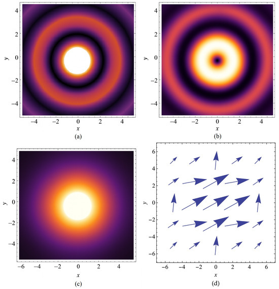
Optical vortices in both components $A_x$ and $A_y$ of the modulated optical wave are illustrated, the total intensity is presented, as well as the vector diagram in the laser radiation spot at $\zeta =0$ and for different values of the vortex parameter n.

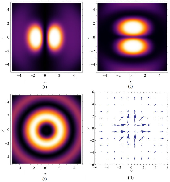
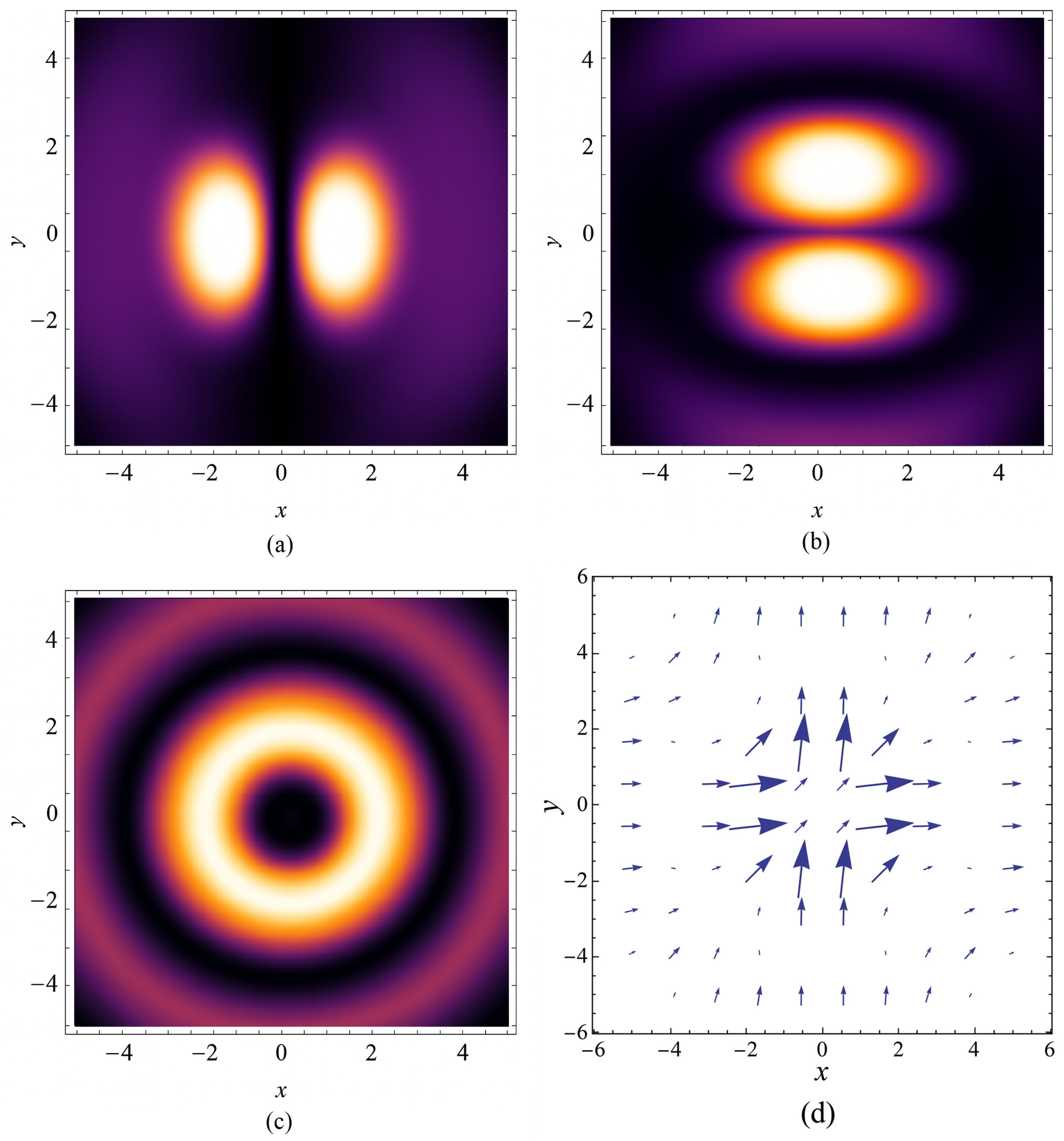
The vortex structures in the components of the modulated optical wave, the total intensity, as well as the vector diagram at $\zeta =0$ and $n=1$ are shown in Figure 1. Two bright spots are clearly visible in the components of the amplitude function. In the total intensity, however, a characteristic ring-shaped structure with a dark central spot due to the Bessel function is observed. As the vortex parameter n increases, its radius grows.

Figure 1. Optical vortices observed in the (a) $A_x$ component and the (b) $A_y$ component of the modulated optical wave; (c) the total intensity; (d) the vector diagram at $\zeta =0$ and $n=1$.

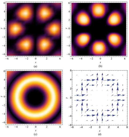
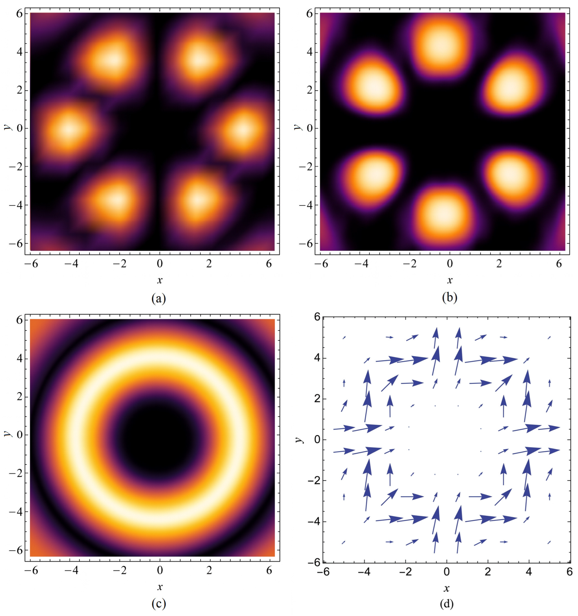
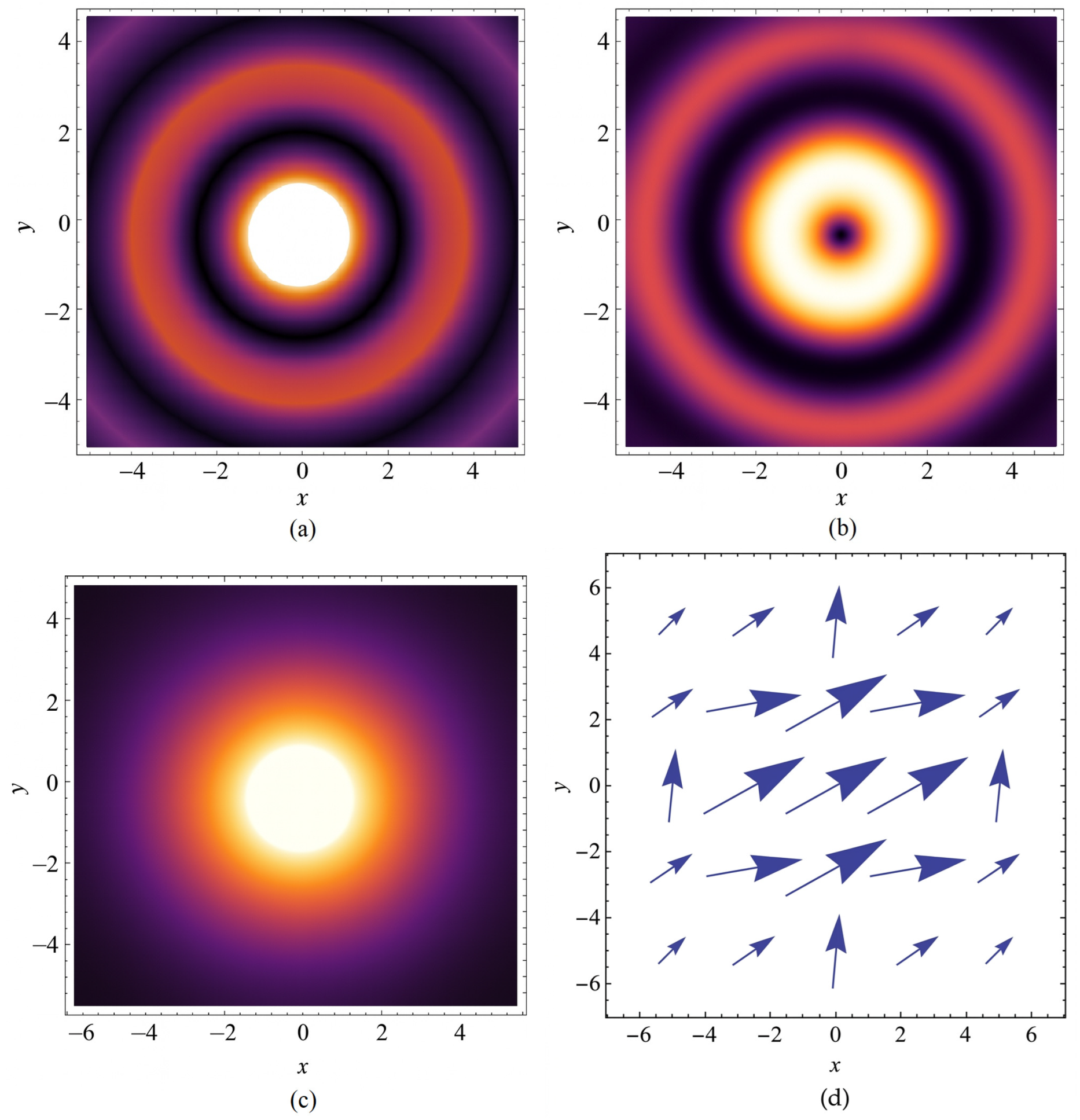
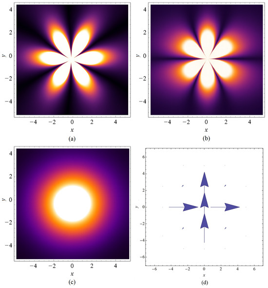
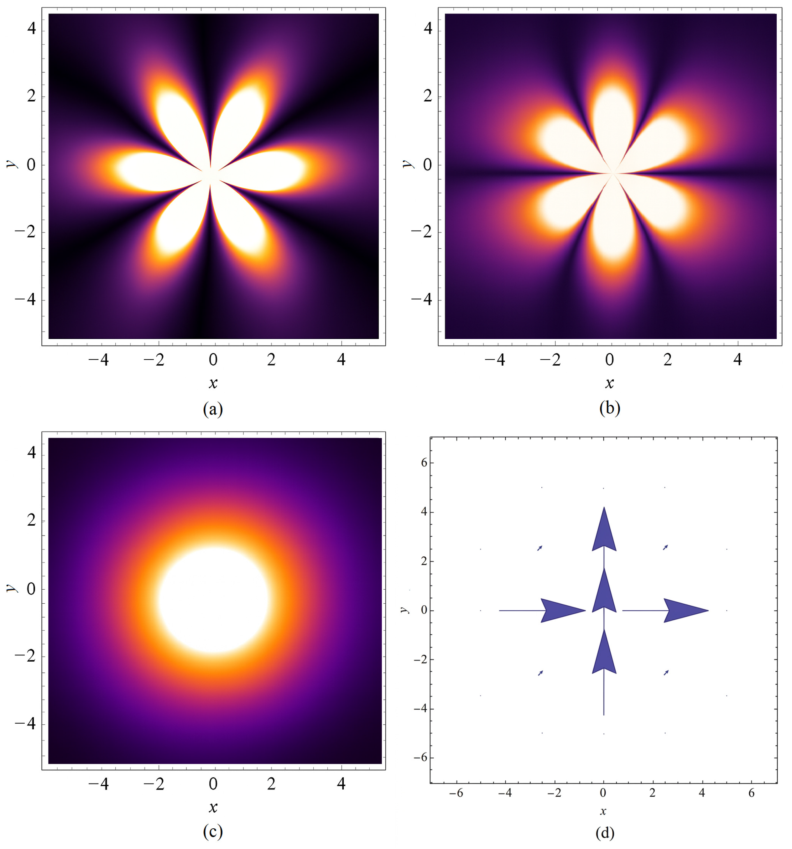
Optical vortex structures in the components of the modulated optical wave, its total intensity, as well as the vector diagram at $\zeta =0$ and $n=3$ are shown in Figure 2. It is interesting to note that in this case a “necklace” of bright spots arranged in a circle is observed. Their number is six, which corresponds to the doubled value of the vortex parameter $2n$. The total intensity of the wave is again composed of concentric rings with a dark central spot. The vector diagram becomes more complicated.

Figure 2. Optical vortices observed in the (a) $A_x$ component and the (b) $A_y$ component of the modulated optical wave; (c) the total intensity; (d) the vector diagram at $\zeta =0$ and $n=3$.

The same analogy can be found at higher values of the vortex parameter, but the bright elements in the components of the modulated optical wave are numerous. The total intensity is always in the form of concentric circles with a dark central spot, the radius of which grows with increasing the value of n. The corresponding vector diagrams demonstrate a high degree of rotation of the polarization in the spot of the laser light.

The figure below shows optical vortices in the case where the square of the amplitudes of the two components $A_x$ and $A_y$ of the laser radiation are represented by the following expressions:

$$\begin{array}{c}\hfill \mid A_x{\mid }^2={\left({\displaystyle \frac{1}{\sqrt{r}}}cos\left(r\right)cos\left(\zeta \right)\right)}^2,\end{array}$$

(95)

$$\begin{array}{c}\hfill \mid A_y{\mid }^2={\left({\displaystyle \frac{1}{\sqrt{r}}}sin\left(r\right)cos\left(\zeta \right)\right)}^2.\end{array}$$

(96)

From the given solutions it is clearly seen that the vortex parameter does not participate in the formulas above.

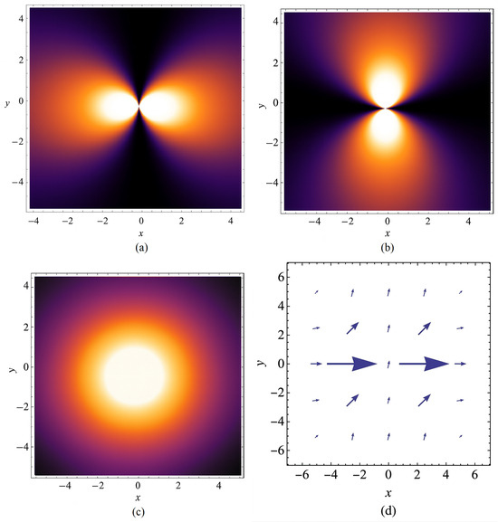
Figure 3 illustrates the typical ring-shaped structure for the amplitude-type vortices, observed in the two components of the vector amplitude function.

Figure 3. Optical vortices observed in the (a) $A_x$ component and the (b) $A_y$ component of the modulated optical wave; (c) the total intensity; (d) the vector diagram at $\zeta =0$.

As it can be seen, the minima in the $A_x$ component coincide with the maxima in the $A_y$ component. Therefore, no vortex structures are detected in the total intensity of the laser radiation. The optical vortex is registered only by the rotation of the polarization of the electric field in the vector diagram.

As a next step, we will consider the solutions obtained when the separation constant is zero $(C=0)$. We assume that the ratio of the constants $M/N=1$.

The next few figures show optical vortices in the case where the square of the amplitudes of the two components $A_x$ and $A_y$ of the modulated optical wave are presented by the following expressions:

$$\begin{array}{c}\hfill \mid A_x{\mid }^2={\left({\displaystyle \frac{1}{\sqrt{r^n}}}cos(m+n\theta )cos\left(\zeta \right)\right)}^2,\end{array}$$

(97)

$$\begin{array}{c}\hfill \mid A_y{\mid }^2={\left({\displaystyle \frac{1}{\sqrt{r^n}}}sin(m+n\theta )cos\left(\zeta \right)\right)}^2.\end{array}$$

(98)

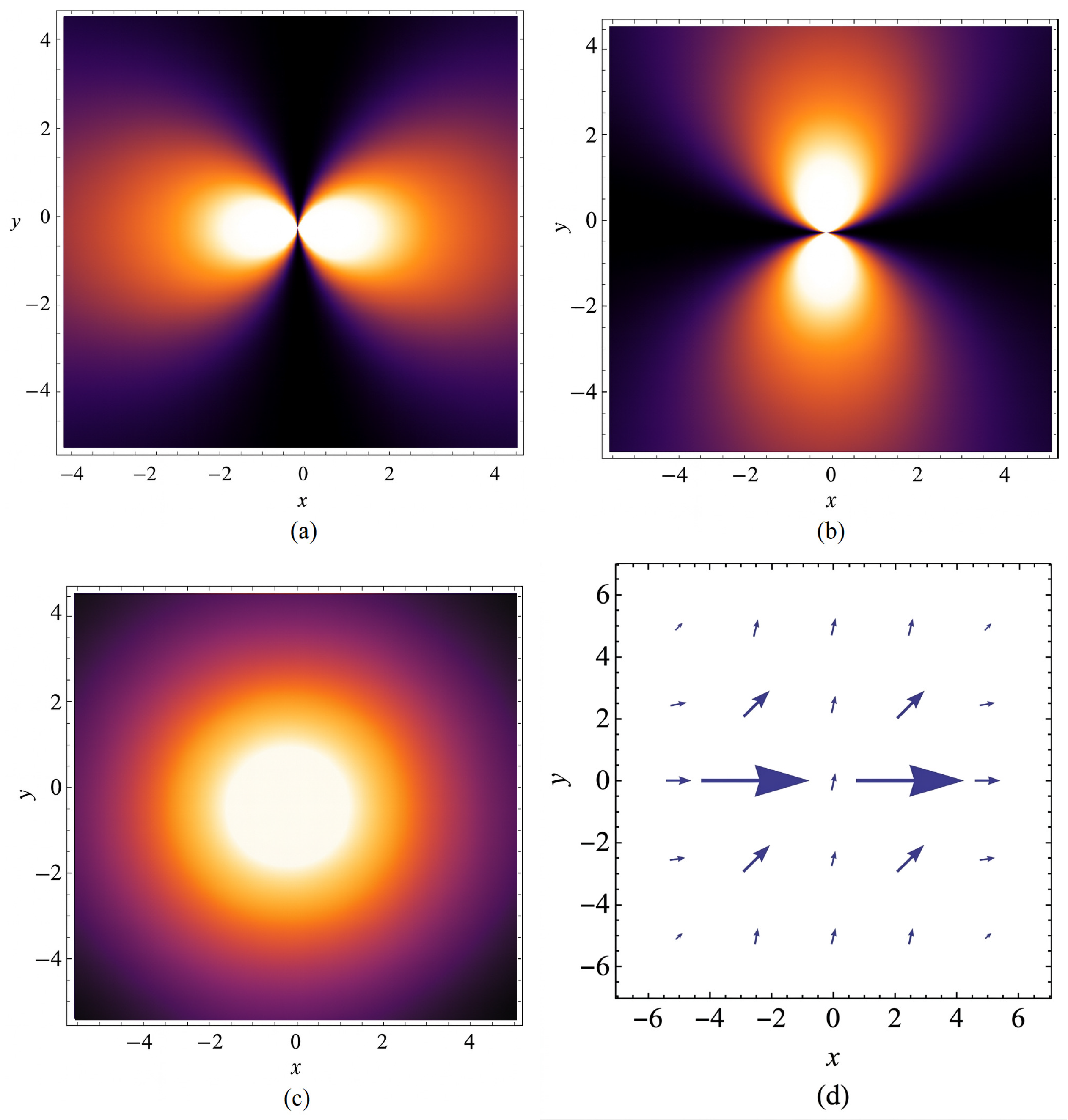
We assume that the modulated optical waves have no initial phase, i.e., $m=0$. Laser vortices at $\zeta =0$ and different values of the vortex parameter n are illustrated. Figure 4 demonstrates the case in which $n=1$.

Figure 4. Optical vortices observed in the (a) $A_x$ component and the (b) $A_y$ component of the modulated optical wave; (c) the total intensity; (d) the vector diagram at $m=0$ and $n=1$.

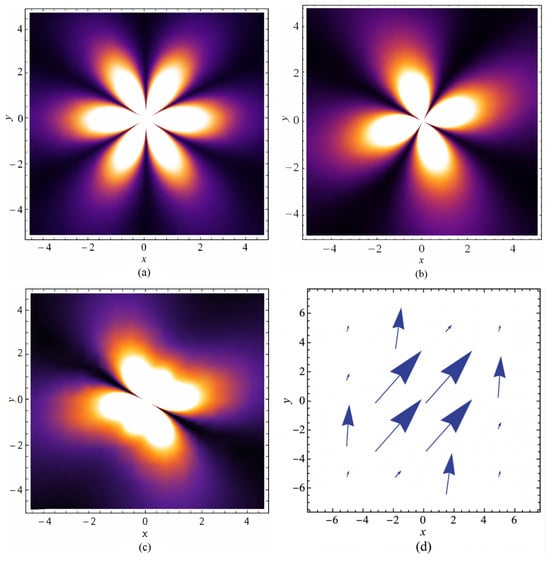
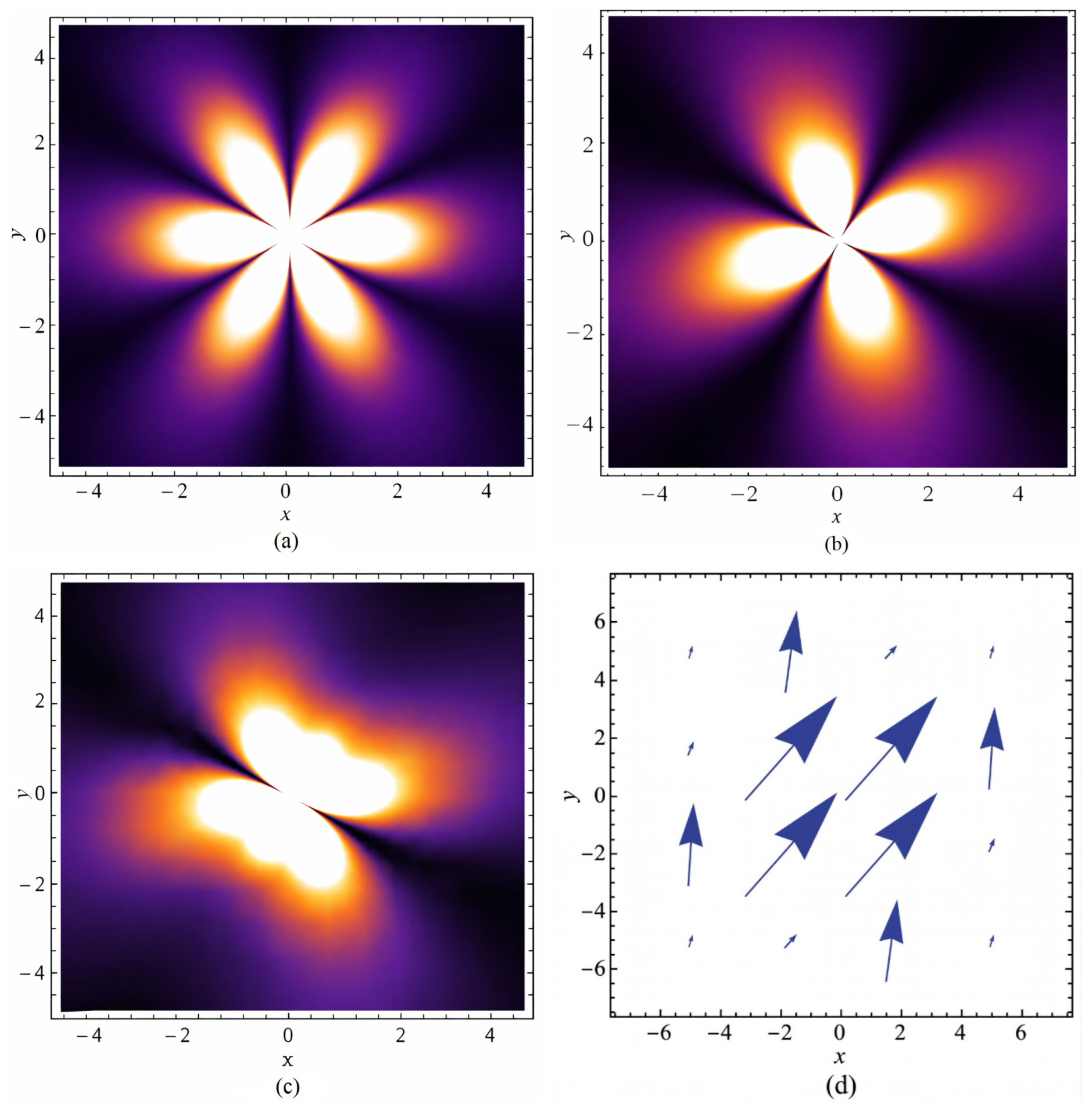
Figure 5 presents the case in which $m=0$ and $n=3$. Here, again the number of bright spots in the vortex structures of the laser light components corresponds to $2n$.

Figure 5. Optical vortices observed in the (a) $A_x$ component and the (b) $A_y$ component of the modulated optical wave; (c) the total intensity; (d) the vector diagram at $m=0$ and $n=3$.

The vector diagrams clearly demonstrate the degree of the rotation in the polarization of the optical field. With increasing value of the vortex parameter, the vortex structures and the vector diagrams become much more complex.

4. Discussions

In our earlier studies, it was demonstrated that laser vortices can also be generated in optical fibers with different refractive index profiles [12]. In particular, fibers with a concave refractive index profile support the formation of helical vortex structures, which arise due to the specific distribution of the refractive index in the medium. These results complement our later investigations for isotropic media, where the propagation of ultra-short laser pulses was shown to produce polarization vortices in the amplitude components $A_x$ and $A_y$, forming concentric ring-like structures [13,14,15].

For the analytical solutions (95) and (96), the maxima of the field of the $A_x$ component coincide with the minima of the field of the $A_y$ component, resulting in a homogeneous total intensity without clearly distinguishable vortex features. In the present study, however, we report new exact analytical solutions that lead to precise control of the parameters of the generated optical vortex structure. In particular, solutions (93) and (94), expressed through Bessel functions, represent oval-shaped elements in the amplitude components (Figure 1a,b), which are mutually shifted, so that their superposition forms the well-known ring-like structures in the total intensity (Figure 1c and Figure 2c). The vortex parameter n plays a decisive role, determining both the number ($2n$) and the complexity of the structural elements. For example, at $n=3$, a complex vortex structure is formed (Figure 2). The number of vortex elements in the intensity profile for each component is six. The vortex parameter can be considered as an analogue of the topological charge in phase vortices, but its physical meaning for polarization vortices is different. It is important to note that in the superposition of two phase vortices with opposite topological charges, they annihilate. In our case, the parameter n has the same sign for the vortices in both components of the wave, as a result of which they compensate each other. Unlike the topological charge, in our solutions n can also take non-integer values. Numerical simulations based on our solutions show that optical vortices are formed even with fractional values of the vortex parameter. They possess a similar structure and resulting spatial intensity distribution.

Additional solutions (97) and (98) lead to another class of vortex structures, where the total intensity appears as a single bright spot (Figure 4 and Figure 5), rather than as a ring-like distribution, while the polarization vortices remain confined only to the amplitude components. The corresponding vector diagrams clearly demonstrate the rotation in the polarization of the electric field, confirming the presence of polarization vortices. Figure 4 and Figure 5 present vortex structures obtained from the exact analytical solutions (97) and (98). These solutions further increase the diversity of possible vortex formations, since their shape and complexity depend not only on the parameter n but also on the additional parameter m, connected with the initial phase of the components of the modulated optical wave. In this case, n defines the complexity of the vortex structure of $A_x$ and $A_y$ and m defines the rotation of the bright elements in the intensity profile of each component.

The important thing in our analytical solutions for the two components of the optical field is that they are independent. Therefore, through the initial conditions we can choose appropriate values of the parameters m and n, so as to control very precisely the profile of the total intensity of the laser light. We have presented graphs for the same values of the parameters m and n for both components of the wave, in which a homogeneous distribution of the intensity in the cross section of the beam is observed. However, this is not necessarily for all possible cases. Different values of the parameters m and n can be chosen for the two solutions, as a result of which complex optical structures will be observed in the total intensity field (Figure 6).

Figure 6. Optical vortices observed in the (a) $A_x$ component ($m=0$ and $n=3$) and the (b) $A_y$ component ($m={\displaystyle \frac{\pi }{3}}$ and $n=2$); (c) the total intensity; (d) the vector diagram of the modulated optical wave.

Overall, the present results not only extend our previous findings but also reveal a controllable mechanism, through the vortex parameter n, for generating diverse vector vortex structures with increasing complexity, offering promising opportunities for different optical applications.

5. Conclusions

In the present paper, a mathematical algorithm for finding exact analytical solutions to the linear vector amplitude equation, describing the propagation of modulated optical wave in isotropic media, is developed. It is reduced to a system of scalar equations for the two components of a laser light. Each of them represents a second-order partial differential equation. They are solved by the method of separation of variables, where C is the constant of separation of variables. Depending on its value ($C\ne 0$ and $C=0$), different types of solutions are found for the two components of the vector amplitude function. Some of them are represented by Bessel functions. In the cross section of these components, amplitude vortices with a complex structure, depending on the value of the vortex parameter n, are formed. The number of repeating elements in the vortex structures corresponds to the doubled value of the vortex parameter $2n$. By increasing the value of n, the vortex structures and vector diagrams become significantly more complex. The presented vector diagrams convincingly prove the presence of optical vortex structures in the optical field. The parameter m is connected with the initial phase of the modulated optical wave’s components. It defines the degree of rotation of the bright elements in the intensity profile of each component. By allowing for arbitrary tuning of the two key parameters n and m, the model provides a flexible platform for generating a variety of vortex structures, complementing the capabilities of standard phase modulation.

The presented model offers a unified description of the generation of vector vortex structures in dispersive media and shows how complex amplitude vortices and polarization singularities can be engineered using exact analytical solutions. These results contribute to the theoretical foundation of singular optics and provide a flexible tool for manipulating structured laser fields in optical systems.

The development of new analytical solutions for modulated vector optical fields represents a significant step toward addressing the widespread challenges of scalable and precise control over complex modes. By enabling exact management of amplitude-type singularities and polarization patterns through parameters like vortex parameter n, this model provides the theoretical foundation needed for high-dimensional information encoding and enhanced sensitivity in metrology [26]. In practical terms, these analytical models offer a clearer path for building more reliable communication systems and optical devices [27,28]. Future work can use these diffraction-free patterns to improve how light travels through tricky environments, such as biological tissues or turbulent air, without losing its shape, opening new possibilities for smaller, more efficient sensors and communication chips [29,30].

References

- Nye, J.F.; Berry, M.V. Dislocations in wave trains. Proc. R. Soc. Lond. A Math. Phys. Sci. 1974, 336, 165–190. [Google Scholar] [CrossRef] [Scilit]
- Allen, L.; Beijersbergen, M.W.; Spreeuw, R.J.; Woerdman, J.P. Orbital angular momentum of light and the transformation of Laguerre-Gaussian laser modes. Phys. Rev. A 1992, 45, 8185. [Google Scholar] [CrossRef] [Scilit] [PubMed]
- Tidwell, S.C.; Ford, D.H.; Kimura, W.D. Generating radially polarized beams interferometrically. Appl. Opt. 1990, 29, 2234–2239. [Google Scholar] [CrossRef] [Scilit]
- Shen, Y.; Wang, X.; Xie, Z.; Min, C.; Fu, X.; Liu, Q.; Gong, M.; Yuan, X. Optical vortices 30 years on: OAM manipulation from topological charge to multiple singularities. Light. Sci. Appl. 2019, 8, 90. [Google Scholar] [CrossRef] [Scilit]
- Soskin, M.S.; Vasnetsov, M.V. Singular optics. Prog. Opt. 2001, 42, 219–276. [Google Scholar] [CrossRef] [Scilit]
- Dennis, M.R.; O’Holleran, K.; Padgett, M.J. Singular optics: Optical vortices and polarization singularities. Prog. Opt. 2009, 53, 293–363. [Google Scholar] [CrossRef] [Scilit]
- Bekshaev, A.Y.; Soskin, M.S.; Vasnetsov, M.V. Paraxial light beams with angular momentum. arXiv 2008, arXiv:0801.2309. [Google Scholar] [CrossRef] [Scilit]
- Bezuhanov, K.; Dreischuh, A.; Paulus, G.G.; Schätzel, M.G.; Walther, H. Vortices in femtosecond laser fields. Opt. Lett. 2004, 29, 1942–1944. [Google Scholar] [CrossRef] [Scilit]
- Stoyanov, L.; Zhekova, M.; Stefanov, A.; Stefanov, I.; Paulus, G.G.; Dreischuh, A. Zeroth- and first-order long range non-diffracting Gauss–Bessel beams generated by annihilating multiple-charged optical vortices. Sci. Rep. 2020, 10, 21981. [Google Scholar] [CrossRef] [Scilit]
- Wang, X.; Nie, Z.; Liang, Y.; Wang, J.; Li, T.; Jia, B. Recent advances on optical vortex generation. Nanophotonics 2018, 7, 1533–1556. [Google Scholar] [CrossRef] [Scilit]
- Marrucci, L.; Manzo, C.; Paparo, D. Optical spin-to-orbital angular momentum conversion in inhomogeneous anisotropic media. Phys. Rev. Lett. 2006, 96, 163905. [Google Scholar] [CrossRef] [Scilit] [PubMed]
- Slavchev, V.; Dakova, A.; Bojikoliev, I.; Dakova, D.; Kovachev, L. Helical vortex structures and depolarization in fiber with concave-gradient profile. Optik 2021, 242, 167124. [Google Scholar] [CrossRef] [Scilit]
- Slavchev, V.; Dakova, A.; Gocheva, N.; Bozhikoliev, I.; Kovachev, K.; Biswas, A. Laser ring structures in step-index fibers. J. Phys. Conf. Ser. 2022, 2339, 012007. [Google Scholar] [CrossRef] [Scilit]
- Slavchev, V.; Dakova, A.; Dakova, D.; Bozhikoliev, I.; Kovachev, L.; Biswas, A. New vector type optical vortex structures in isotropic media. J. Phys. Conf. Ser. 2023, 2487, 012030. [Google Scholar] [CrossRef] [Scilit]
- Slavchev, V.; Bozhikoliev, I.; Zamanchev, Z.; Dakova, A.; Kovachev, K.; Biswas, A. Optical vortices in waveguides with spatial dependence of the nonlinear refractive index. Opt. Quantum Electron. 2022, 54, 346. [Google Scholar] [CrossRef] [Scilit]
- Freund, I. Polarization flowers. Opt. Commun. 2001, 199, 47–63. [Google Scholar] [CrossRef] [Scilit]
- Nye, J. Dislocations and disclinations in transverse electromagnetic waves. In Physics of Defects; Balian, R., Kleman, M., Poirier, J.-P., Eds.; North-Holland: Amsterdam, The Netherlands, 1981; pp. 545–549. [Google Scholar]
- Berry, M.V.; Dennis, M.R. Polarization singularities in isotropic random vector waves. Proc. R. Soc. Lond. A 2001, 457, 141–155. [Google Scholar] [CrossRef] [Scilit]
- Nye, J.F. Polarization effects in the diffraction of electromagnetic waves: The role of dislocations. Proc. R. Soc. Lond. A 1983, 387, 105–132. [Google Scholar] [CrossRef] [Scilit]
- Jiang, J.-J.; Zhuang, K.-H.; Chen, J.-D.; Li, J.-X.; Chen, Y.-Y. Controlling the Polarization and Vortex Charge of γ Photons via Nonlinear Compton Scattering. Phys. Rev. Lett. 2025, 134, 153802. [Google Scholar] [CrossRef] [Scilit]
- Boyd, R.W. Nonlinear Optics, 3rd ed.; Academic Press: San Diego, CA, USA, 2003. [Google Scholar]
- Agrawal, G.P. Nonlinear Fiber Optics; Academic Press, Inc.: New York, NY, USA, 2008. [Google Scholar]
- Arfken, G.B.; Weber, H.J.; Harris, F.E. Mathematical Methods for Physicists: A Comprehensive Guide, 7th ed.; Academic Press: Waltham, MA, USA, 2012. [Google Scholar] [CrossRef] [Scilit]
- Evans, L.C. Partial Differential Equations, 2nd ed.; Graduate Studies in Mathematics; American Mathematical Society: Providence, RI, USA, 2010; Volume 19, 749p. [Google Scholar]
- Soskin, M.S.; Gorshkov, V.N.; Vasnetsov, M.V.; Malos, J.T.; Heckenberg, N.R. Topological charge and angular momentum of light beams carrying optical vortices. Phys. Rev. A 1997, 56, 4064. [Google Scholar] [CrossRef] [Scilit]
- Balasubramaniam, G.M.; Allam, S.R.; Anand, V.; Ansari, M.H.; Arockiaraj, F.G.; Arnon, S.; Badavath, P.S.; Baliyan, M.; Bouchal, P.; Bouchal, Z.; et al. Roadmap on singular optics and its applications. Appl. Phys. B 2026, 132, 58. [Google Scholar] [CrossRef] [Scilit] [PubMed]
- Zhang, H.; Zeng, J.; Lu, X.; Wang, Z.; Zhao, C.; Cai, Y. Review on fractional vortex beam. Nanophotonics 2022, 11, 241–273. [Google Scholar] [CrossRef] [Scilit] [PubMed]
- Wang, J. Advances in communications using optical vortices. Photon. Res. 2016, 4, B14–B28. [Google Scholar] [CrossRef] [Scilit]
- Fang, G.J.; Pu, J.X. Propagation properties of stochastic electromagnetic double-vortex beams in a turbulent atmosphere. Chin. Phys. B 2012, 21, 084203. [Google Scholar] [CrossRef] [Scilit]
- Ritsch-Marte, M.; Bernet, S.; Jesacher, A.; Fürhapter, S.; Maurer, C.; Schwaighofer, A. Singular Optics for Novel Biomedical Tools. In Conference on Coherence and Quantum Optics; OSA Technical Digest (CD), Paper CME3; Optica Publishing Group: Washington, DC, USA, 2007. [Google Scholar] [CrossRef] [Scilit]
Disclaimer/Publisher’s Note: The statements, opinions and data contained in all publications are solely those of the individual author(s) and contributor(s) and not of MDPI and/or the editor(s). MDPI and/or the editor(s) disclaim responsibility for any injury to people or property resulting from any ideas, methods, instructions or products referred to in the content. |
© 2026 by the authors. Licensee MDPI, Basel, Switzerland. This article is an open access article distributed under the terms and conditions of the Creative Commons Attribution (CC BY) license.