An SVM-Based High-Precision Reconstruction Algorithm for High-Power Laser Beam Spots with Large Divergence Angles

Abstract

Lasers are a key enabling technology across numerous engineering and scientific fields, especially in high-energy laser systems for defense, materials processing, and fusion research, where precise characterization of high-power, large-divergence-angle laser spots is critical. However, the inherent properties of high-power, large-divergence-angle lasers—such as large spot area and strong intensity contrast—pose real obstacles to existing methods, which often suffer from low accuracy and inefficiency. In this paper, a flat-field correction technique was proposed for the CCD to reduce the distortions produced by the non-uniform response of the sensor in spot measurements. Then, a spot recognition algorithm based on support vector machines was developed, which can effectively and accurately locate and identify laser spots with limited training samples and computational resources, achieving a classification accuracy of over 98.11%. Additionally, an efficient correction approach is proposed to assess the spot intensity and shape with high accuracy even at large tilt angles. Experimental results show that this proposed approach can measure the high-power laser spot with a large divergence angle precisely and efficiently, and improves both the measurement precision and operational efficiency remarkably.

1. Introduction

As a reliable and highly controllable light source, the applications of lasers can be found in position location, dimensional measurement, and three-dimensional reconstruction. Nevertheless, non-ideal properties in the optical system itself, lens vignetting [1,2,3], the non-uniform responsivity of the CCD sensor [4,5,6], and the angle of incidence [7,8]—frequently lead to common imaging distortions, including light spots [9,10], luminance non-uniformity [11,12], and geometric distortion [13], which severely impact the accuracy of the measurement. Therefore, it is important to obtain the precise characterization of a laser spot in order to improve the accuracy of vision measurement systems based on laser vision sensors.

Recent advancements in laser measurement technology have yielded significant progress across multiple technical fronts. Gaussian fitting applied to laser spot images has enabled precise manipulation of optical assembly measurements in large LiDAR systems, facilitating more accurate alignment and calibration of optical components [14]. The integration of collimation techniques has markedly improved beam quality measurement accuracy, reducing M² deviation to below 0.6% [15]. CCD-based methodologies have achieved arcsecond-level zero-drift measurements in optical sights with exceptional angular stability assessment capabilities [16]. Multi-focal-plane-constrained coherent modulation imaging has enabled simultaneous measurement of near-field and focal-spot intensity distributions, advancing comprehensive laser beam characterization [17]. A novel spatial-scanning hyperspectral imaging system utilizing rotating slits and Dove prisms has been developed [18], while in-plane spin splitting in the photonic spin Hall effect has been exploited for high-precision beam waist estimation [19]. Conically arranged optical fibers with decimeter-scale receiving apertures and millimeter-scale resolution have been proposed for laser parameter measurement [20]. Systematic analysis of speckle noise influence on laser triangulation has resulted in effective suppression strategies [21], and optimization of temperature-induced laser spot centroid drift has achieved positioning accuracy of 3.6 μm [22]. Image fusion techniques have enabled effective measurement of far-field divergence angles [23], while phase-retrieval methods applied to liquid lenses have improved M² measurement efficiency [24], complemented by dual linear-array CCD systems for effective infrared divergence angle measurement [25]. Multi-laser displacement sensors and transport-of-intensity equations have contributed to surface-normal measurements and complex-amplitude reconstruction of beam quality, respectively [26,27]. The fusion of piecewise polynomial fitting with Kalman filtering has enhanced quadrant-detector tracking accuracy [28], and quadratic models describing temperature–spot centroid drift relationships have improved understanding of optical sensor environmental adaptability [29]. By optimizing the detection window combined with high-order moment weighting, accelerating parallel computing on FPGA, and adopting neural network-based technical alternatives, the issues of noise interference, insufficient speed, and multispectral failure in the centroid detection algorithm for laser beam measurement can be effectively improved [30,31,32].

In this paper, we describe a vision-based speckle measurement system and its application to addressing the problem of the method we use to test high-power laser spots. Although research into cutting-edge laser spot measurement has progressed greatly, it has primarily been focused on specific working conditions for particular purposes. There is a clear absence of research pertaining to designing and setting up the optical structure to adequately test quality for high-power and large-divergence-angle laser spots. Three crucial aspects for this topic will be covered, and we will determine the method’s influence on identification precision for all: selection of CCD cameras, installation setup design, and image processing. Measurement difficulties with optical systems are addressed in this paper, and a complete solution is provided. First, the paper introduces a flat-field correction technique for CCD sensors, compensating for the inconsistency of sensor values, which might distort spot values during large-scale spot measurements. Then, the paper proposes an effective spot detection algorithm for image processing, aimed at rapid and correct spot identification for lasers, even when the available training set is small, and the computing capacity is restricted. Finally, the paper puts forward a correction approach for spot shape and brightness, making it possible to measure both geometric spot shape and emission intensity, even at steep incidence angles. In general, the paper deals with extreme parameter values within a whole optical-system design and corresponding detection techniques, which play a vital part in the overall integrated measurement procedure and are strongly needed today.

2. Hardware System Construction

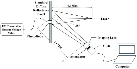
A laser spot measurement system has two components: a laser emission unit and a spot measurement unit. In the laser emission unit, the laser diode used is manufactured by Sharp Corporation, located in Osaka, Japan, model GH04C05Y9G, with a center wavelength of 440 nm, an output power of 5 W, and a continuous-wave (CW) operating mode. According to the datasheet, the output beam dimensions (waist radii) at the laser aperture are approximately 0.37 µm for the fast axis and 1.60 µm for the slow axis. The beam divergence angles (full width at $1\backslash e^2$) are typically 43° for the fast axis and 10° for the slow axis. The output polarization is linearly polarized (TE mode). The beam quality factors M_x² and M_y² will be measured and calculated in subsequent experiments to further characterize the beam quality. In the spot measurement unit, there is a diffuse-reflection plate, a silicon photo-diode, an imaging lens, a CCD camera, and a data processing unit. The standard diffuse-reflection plate used in this experiment is manufactured by Ruike Optoelectronics, Guangzhou, China, model RK-WB. It is made of PTFE material and has a reflectance of up to 99% across the 200–2500 nm wavelength range. The plate features Lambertian scattering characteristics, meaning the reflected radiance remains constant for all angles of illumination and views. Therefore, it is well-suited for reflectance calibration and response uniformity correction of optical systems such as spectrometers and cameras. The plate has a silicon photodiode that turns light into an electrical current. These currents are further turned into voltages through an I–V conversion circuit, thus directly connecting image intensity in its grayscale levels to actual electrical voltages. The photodiode used is the NSPU1.3-F2 silicon PIN photodiode manufactured by Hangzhou Ningguang Technology Co., Ltd., Hangzhou, China, with a spectral response range of 200–1100 nm and an effective photosensitive area of 1.3 mm × 1.3 mm. The CCD camera is a Mercury II series industrial camera, model MER2-507-23GM-P, produced by Daheng Image, Beijing, China, with a resolution of 2592 × 1944, a pixel size of 2.2 μm × 2.2 μm, and pixel depths supporting 8-bit and 12-bit. The imaging lens is a Computar V5024-MPZ manual iris lens manufactured by Computar Corporation in Tokyo, Japan. It has a focal length of 50 mm, a sensor format of 1 inch, a C-mount interface, and a nominal distortion of 0.0%, indicating good aberration correction. In addition to more accurate measurement results, there are optional specific attenuation filters that suit various applications that are designed to modulate the laser light while reducing spurious light effects. The attenuators used in the experiment are neutral density filters with a typical optical density of OD 2.0, corresponding to a transmittance of 1%. The measurement system shown in Figure 1 was set up with the semiconductor laser diode positioned 0.155 m from the diffuse-reflection plate, the imaging lens located 1.172 m from the diffuse-reflection plate, and the CCD camera capturing the target plane laterally at an angle of 35°.

Figure 1. Visual measurement system based on light spots.

3. CCD Sensor Flat-Field Correction

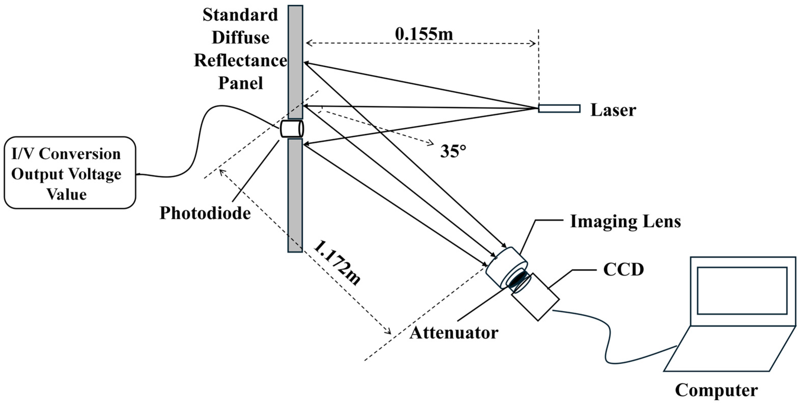
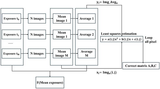
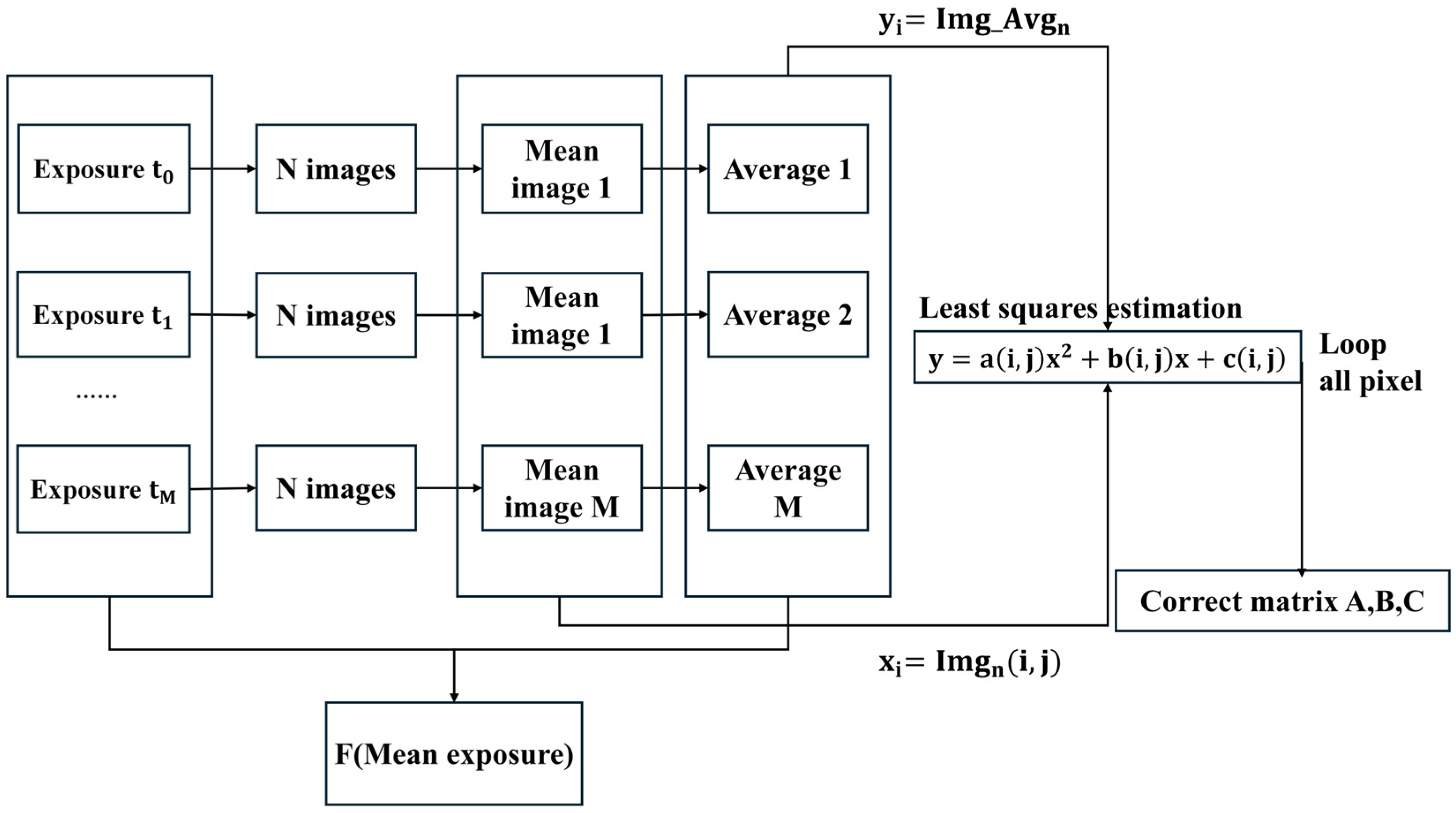
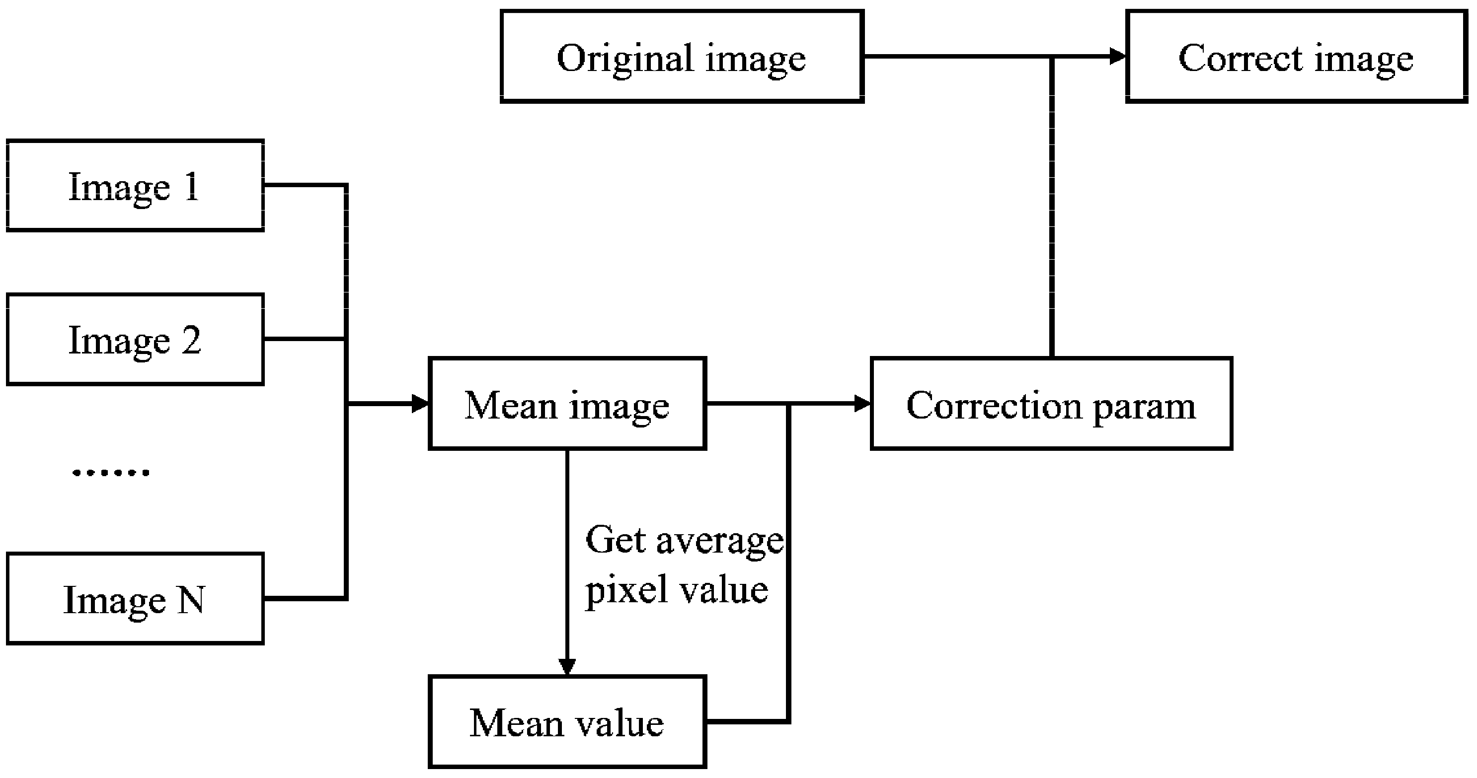
The precision of our measurements depends on two characteristics of the cameras: their signal-to-noise ratio and their uniformity of response across the field. For this reason, camera calibration is crucial for accurate spot measurements. In CCD sensors, pixel-to-pixel variations are usually observed even under perfectly uniform illumination, while the lens also plays a crucial role in the image homogeneity [33]. In order to address these mismatches, this paper proposes a flat-field correction methodology, as illustrated in Figure 2.

Figure 2. Flat-field correction algorithm.

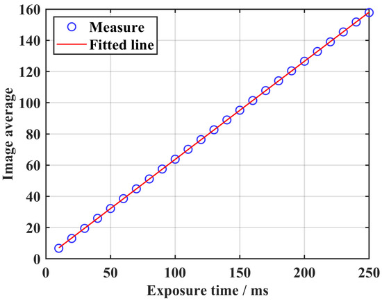
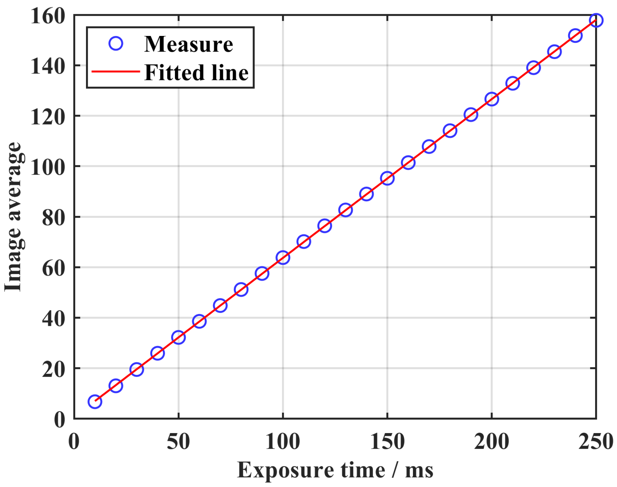
The system response curve is computed as follows: Place the camera so that it takes a uniform white target filling its frame, and shoot five photos at varying exposure times. Once the image is enhanced through time domain averaging, get the average intensity for every image (associated with its respective exposure time), so that an exposure time versus mean intensity is created, and estimate a system response curve through least squares, as shown in Figure 3.

Figure 3. System response curve fitting using least squares.

The image mean is used as a value that represents what is expected from a pixel, while pixel intensity represents what is observed and what is worked with. The connection between what is expected and what is observed is given by

$$\mathrm{y}(\mathrm{i},\mathrm{j})=\mathrm{a}(\mathrm{i},\mathrm{j})\times {\mathrm{x}(\mathrm{i},\mathrm{j})}^2+\mathrm{b}(\mathrm{i},\mathrm{j})\times \mathrm{x}(\mathrm{i},\mathrm{j})+\mathrm{c}(\mathrm{i},\mathrm{j})$$

(1)

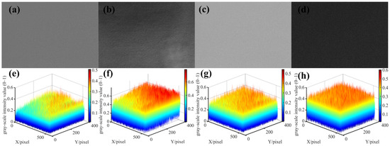
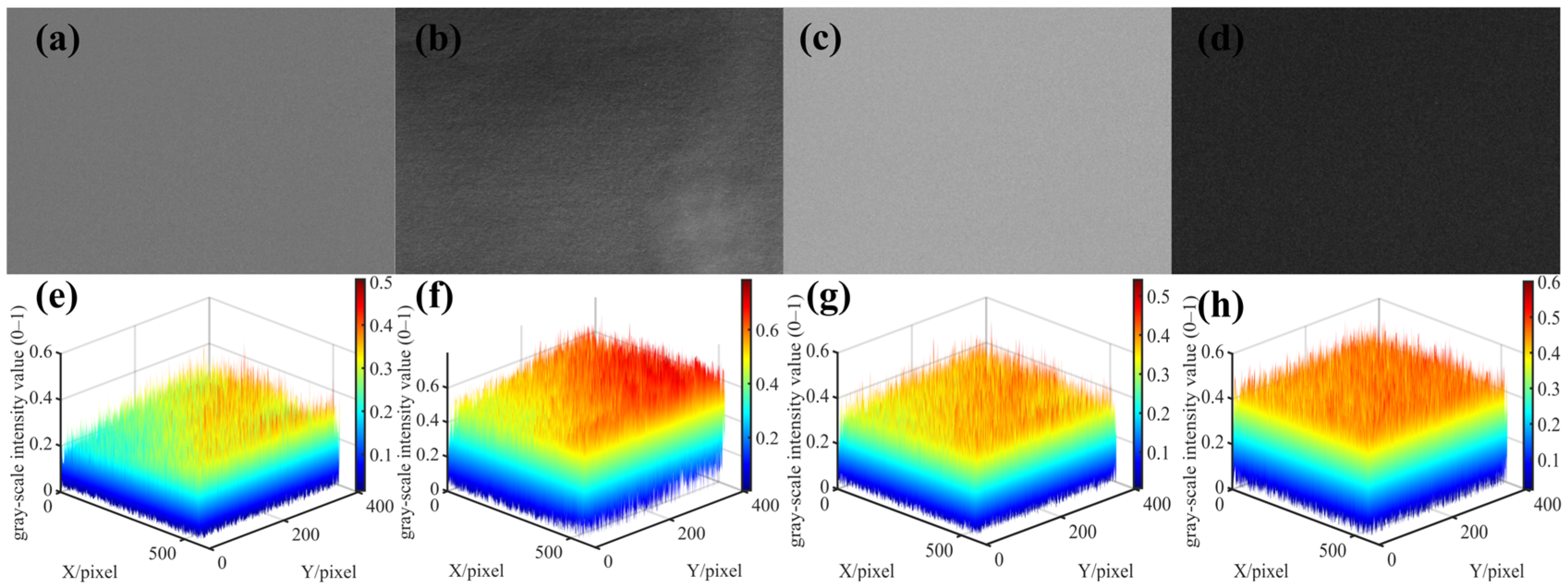
Here, “i” and “j” represent the pixel location, while “a,” “b,” and “c” represent the corresponding elements. A least squares problem is formulated for each pixel to solve for the parameters. In Figure 4, the correction removes the effect of sensitivity variations between the pixels by forcing all pixel responses to the global mean value of the image. Figure 4a–c,e–g present the grayscale images and corresponding 3D surface visualizations of the three final correction coefficient matrices A, B, and C. Figure 4d,h show the grayscale image and corresponding 3D surface visualization of the correction error. It can be observed from the figures that the coefficient matrices are not entirely uniform but exhibit a certain spatial structure. Matrix A (the quadratic coefficient) is generally small in magnitude, but its variation is relatively more pronounced near the edges of the image, reflecting differences in the sensor’s response characteristics within the nonlinear region. Matrix B (the linear coefficient) reveals the response difference between the center and the edge of the sensor, with the central area typically having higher gain and the edges lower gain due to lens vignetting. Matrix C (the constant term) primarily compensates for dark current non-uniformity and circuit offset.

Figure 4. Flat-field correction result. (a–d) Grayscale images; (e–h) Corresponding 3D surface images.

4. Design of the Light Spot Extraction Algorithm

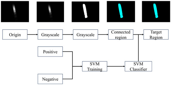
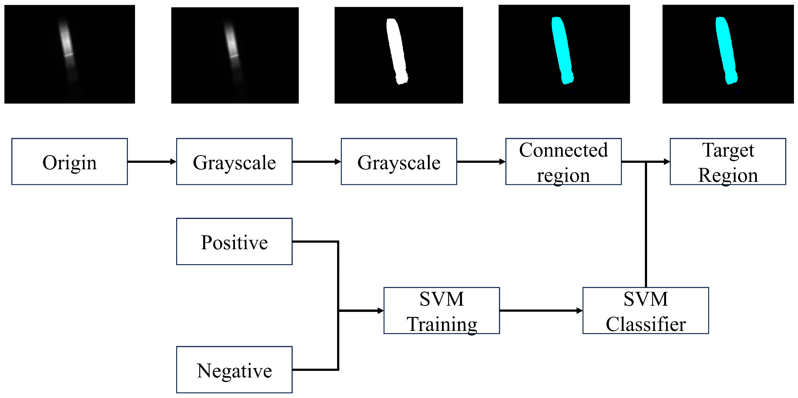
First, we locate and distinguish the laser spot area. The process of image processing is described in Figure 5 and can be summarized as follows: Take the original image and turn it into a grayscale image. Next, the image undergoes a process of optimal global thresholding using the Otsu algorithm, but for the binary platform, 20% of the obtained threshold level is actually applied, producing a binary image with a clearly delimited spot area [34]. Connected component analysis then supplies a number of spots and noise areas. To provide a high level of accuracy during classification, each of these components is resized using a bounding rectangle and then saved as positive (spots) and negative (noises) samples, retaining a complete set of brightness and geometric attributes.

Figure 5. Spot recognition algorithm.

Support vector machines (SVMs) excel at processing samples with a high-dimensional vector, making them fit for this task. The sizes of the light spot and non-light-spot regions may differ greatly. To provide a steady input to the SVM, the images have to be preprocessed for equal dimensions while maintaining aspect ratios. To accomplish this for an image of M × N dimensions, it has to be determined whether M or N needs to be padded and by how many values. The image has to be padded on the shorter side, i.e., min(M,N), by values of max(M,N)−amin(M,N). The image will now be reshaped into a square matrix of max(M,N) × max(M,N) dimensions and then transformed to 128 × 128-resolution images for processing. We assembled a diverse set of light spot images and performed image segmentation based on the light spot area against non-light-spot areas. These light spot areas were labeled as positive samples, while the non-light-spot areas were labeled as negative samples. This yielded a dataset of 199 positives and 230 negatives for a total of 429 images: 343 for training and 86 for validation. The kernel used was linear; thus, these 128 × 128 images were reshaped into a column vector in 1 × 16 × 384 format for training. The best accuracy upon validation was 98.11%.

5. Spot Shape and Intensity Correction

5.1. Spot Shape Correction

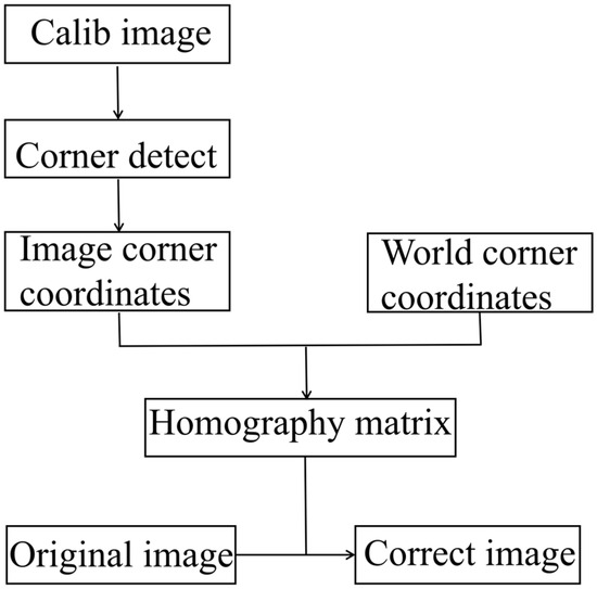
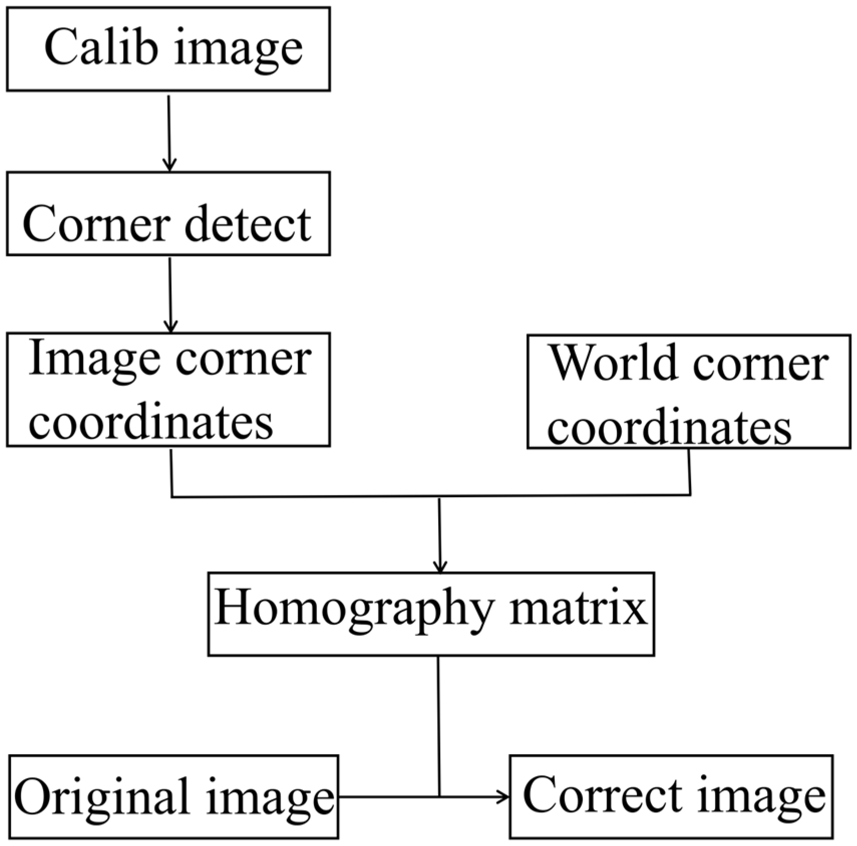
In practical measurement, when mounting the camera, it is difficult to ensure that the optical axis of the camera is strictly perpendicular to the projection surface. If the camera directly captures the image, there might be errors involved in the measurement process due to the perspective effect on the image. Thus, it is necessary to correct the geometric shape of the light spot. Isometric correction is one of the fundamental tools of geometric correction that deals with distortions from images when viewed from an oblique perspective. In this paper, perspective transformation is used to correct the geometric shape. Figure 6 is the algorithm flowchart of perspective transformation.

Figure 6. Perspective transformation correction algorithm.

A homography defines a projective transformation between two 2D planes. Given any point in the image, this matrix provides the equivalent location of that point in the other plane. Also, when an image patch is on a real plane surface, its geometry from two different viewpoints can be represented with precision by a homography, as expressed by Equation (2):

$${\left[\begin{array}{c}\mathrm{u}\\ \mathrm{v}\\ 1\end{array}\right]}_1=\mathrm{H}{\left[\begin{array}{c}\mathrm{u}\\ \mathrm{v}\\ 1\end{array}\right]}_0$$

(2)

Here, “u” and “v” describe the coordinate position of a point on the image, while “H” is the homography matrix.

A chessboard with known dimensions is mounted on the projection plane, and an image of the board is captured by the camera. Corners in the image are detected using a checkerboard detection method. In the experiment, the angle between the camera’s optical axis and the projection surface was set at 35°, with a distance of 1.172 m, which is consistent with the angle and distance between the CCD and the diffuser plate shown in Figure 1.

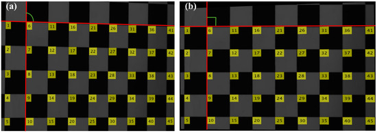
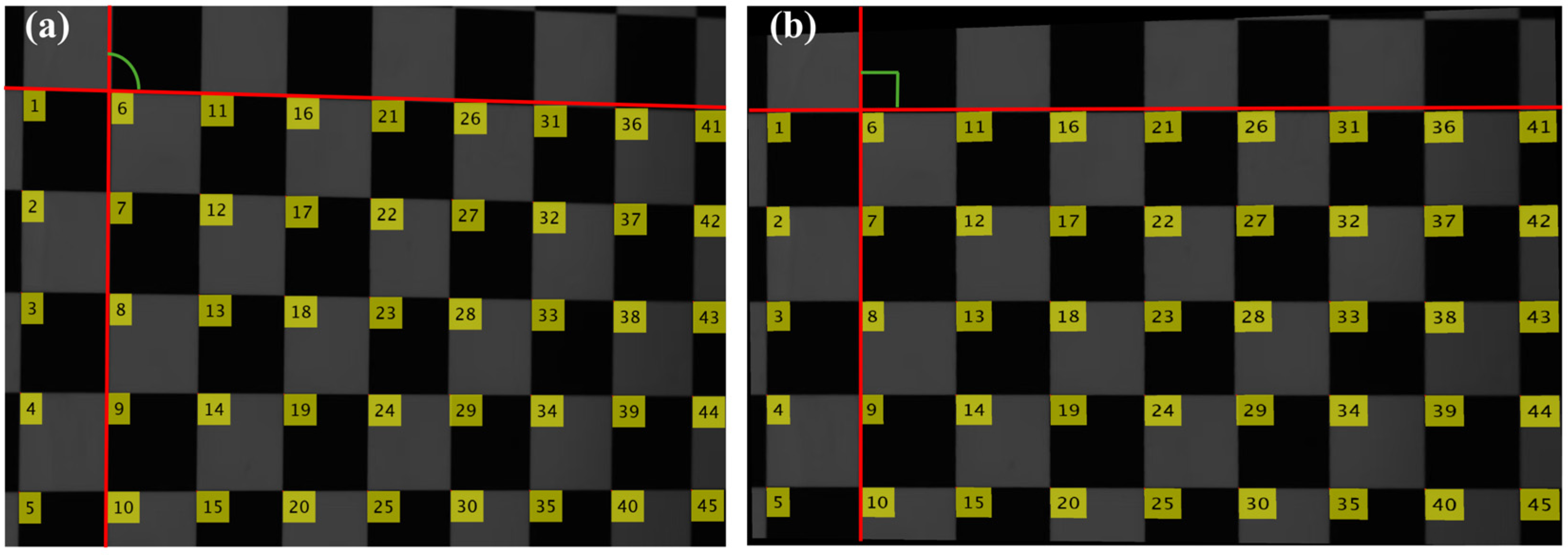
A Cartesian coordinate frame is established with the upper-left corner of the checkerboard at the origin, the larger side of the checkerboard along the X-axis, and the shorter side along the Y-axis. Using measurements, the actual world coordinates of the corners in this reference frame are calculated, providing pairs of image points with their world points, with the relationship between the two systems of points being represented in a 3 × 3 homography matrix, which is calculated using a least squares fit, ensuring an accurate representation of the image world with a reprojection error of 2.48 pixels, as shown in Figure 7 below, showing the difference before and after applying the homography. (a) shows the image before correction, where the distortion of the checkerboard pattern is evident, with the angles appearing as obtuse rather than right angles. (b) shows the image after correction, where the squares in the checkerboard pattern exhibit right angles.

Figure 7. Perspective transformation correction results. (a) Before correction. The numbers indicate the order of the corners, and the red and green lines are added later to highlight the correction effect; (b) After correction.

5.2. Spot Intensity Correction

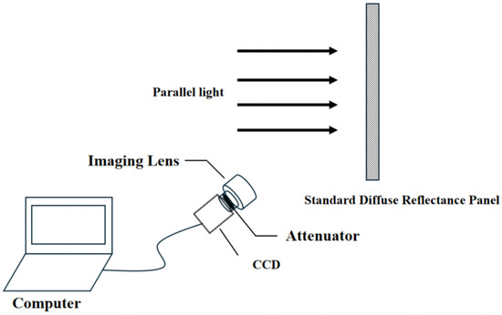
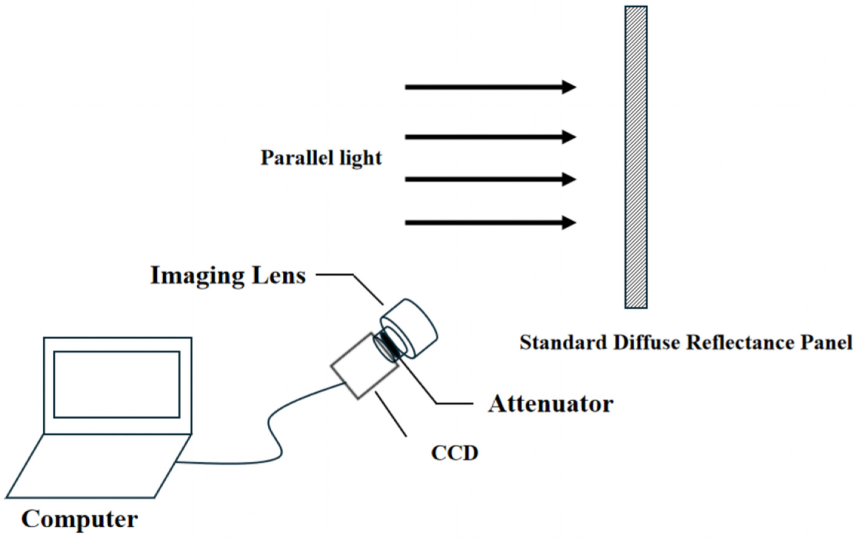
The true illumination pattern is modulated by lens vignetting, stray light, and non-uniform transmittance through the optics. Things are further complicated by considering that the plane of the CCD tilted with respect to the object plane will induce an angular variation of the incident light on the sensor. These result in intensities that differ substantially from the actual distribution of laser irradiance. Therefore, it is necessary to radiometrically correct images by acquiring compensation for geometric effects and system-specific non-uniformities. A parallel beam of light (solar light) illuminates the white diffuse-reflector screen perpendicularly, and the camera captures the reflected radiance along its viewing direction. The angle between the camera’s optical axis and the projection surface was set at 35°, with a distance of 1.172 m. The configuration is illustrated in Figure 8. Figure 9 is the flowchart of the energy correction algorithm.

Figure 8. Spot intensity correction test method.

Figure 9. Energy correction algorithm.

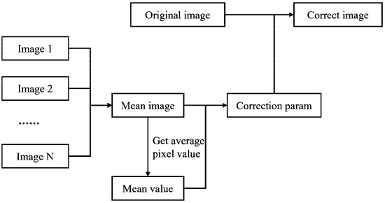
A ten-frame sequence was captured where the reflector was bathed with uniform collimated light. The average frame intensity over all frames on a pixel-by-pixel basis was calculated, representing the reference (optimal) intensity pattern for the white diffuse reflector under normal incidence. The mean image value shows the overall luminance average across all pixels, as shown in Equation (3).

$$\mathrm{V}\mathrm{a}\mathrm{l}\mathrm{u}\mathrm{e}={\displaystyle \frac{1}{\mathrm{h}\times \mathrm{w}}}\sum _{\mathrm{i}=1}^{\mathrm{h}}\sum _{\mathrm{j}=1}^{\mathrm{w}}\mathrm{I}\mathrm{m}\mathrm{g}(\mathrm{i},\mathrm{j})$$

(3)

Here, “Value” represents the average frame brightness value across all frames, while “h” and “w” are the total pixel values of the image’s height and width, respectively.

Under regular lighting conditions, the incident light on the white diffuse reflector is uniform. If the incident light is at an angle, then the intensity varies over space and its distribution can be pre-calculated using the formula provided.

$${\mathrm{I}\mathrm{m}\mathrm{g}}_{\mathrm{C}\mathrm{o}\mathrm{r}\mathrm{r}\mathrm{e}\mathrm{c}\mathrm{t}}(\mathrm{i},\mathrm{j})=\mathrm{V}\mathrm{a}\mathrm{l}\mathrm{u}\mathrm{e}/\mathrm{I}\mathrm{m}\mathrm{g}(\mathrm{i},\mathrm{j})$$

(4)

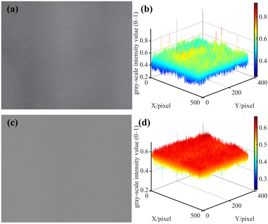
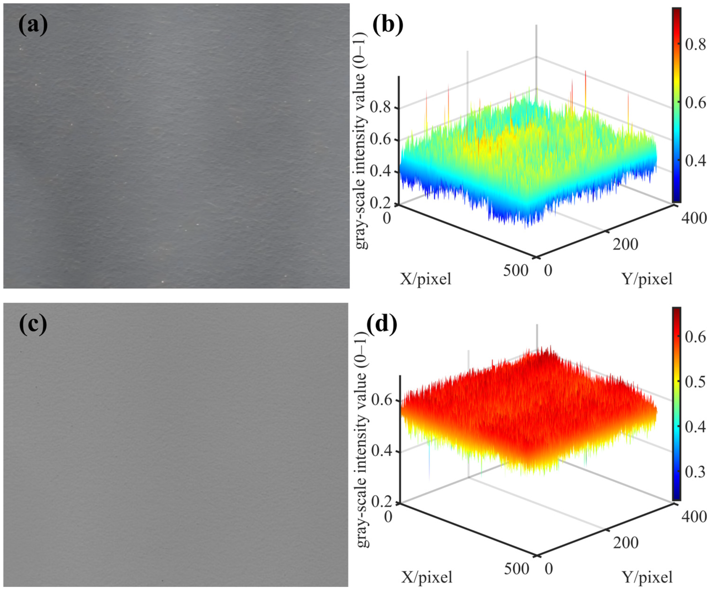
Later, after recording the image of the laser spot, it is multiplied on a pixel-by-pixel basis by the calibrated illumination intensity matrix to produce the radiometrically calibrated power distribution. Figure 10 presents the grayscale image of the captured uniform-white-light image (a) and the image after correction using the computed correction coefficient matrix (c), along with their corresponding 3D surface visualizations (b) and (d).

Figure 10. Spot intensity correction. (a) Grayscale image before correction; (b) 3D surface image before correction; (c) Grayscale image after correction; (d) 3D surface image after correction.

6. Results and Discussion

6.1. Spot Measurement

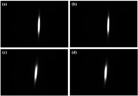
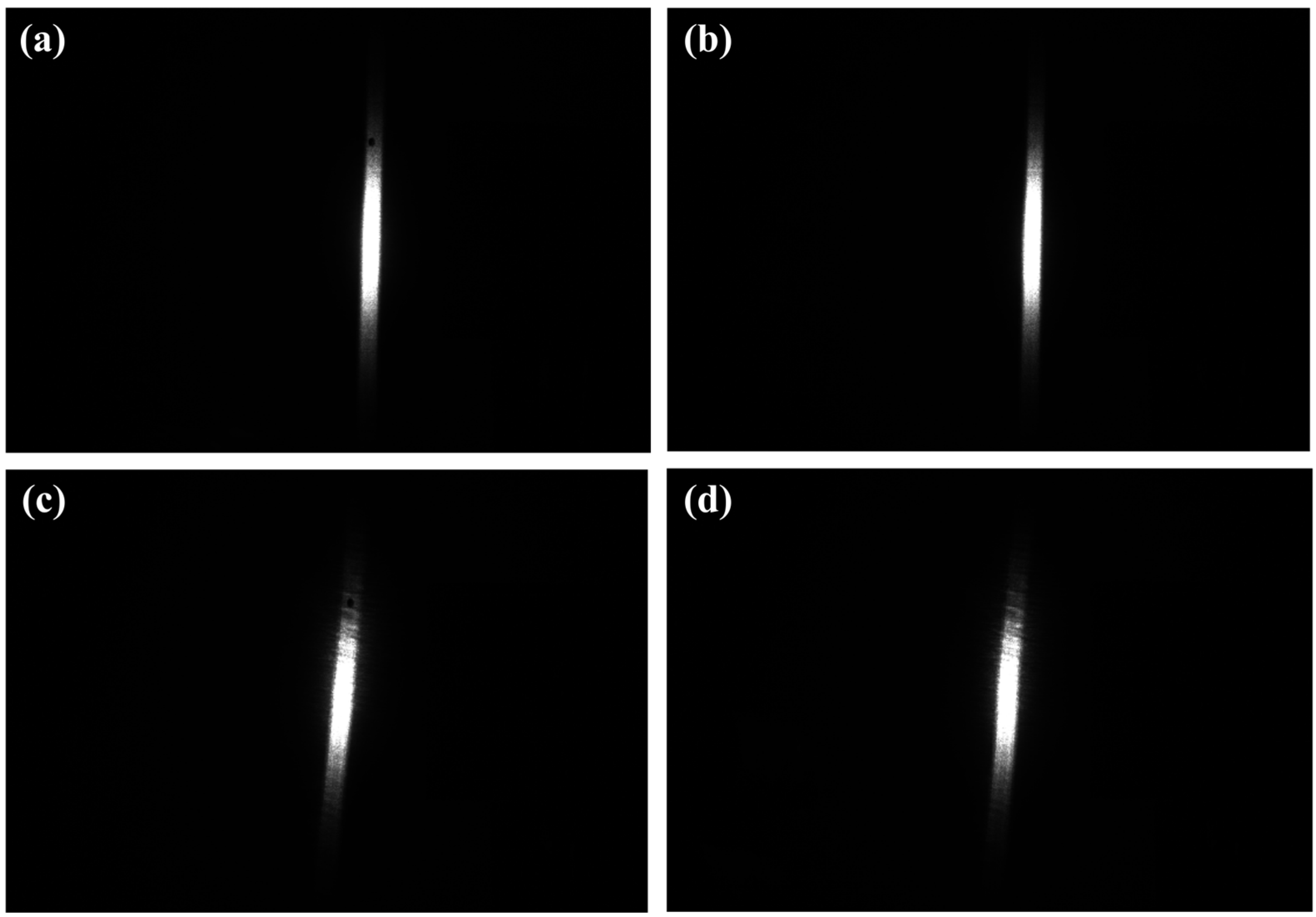
With CCD measurements, what we have is a series of quantized grayscale values provided by the camera that accurately reflect the intensity of the incident light. Then, because we need a calibration that will translate these grayscale values into actual values of optical power, we have to radiometrically calibrate our measurement system. The manner by which we perform our calibration has been mentioned above, with a diffuse-reflector screen that has a hole in it and a calibrated photodiode placed behind it that actually measures the amount of light that goes through. The procedure for calibration is as follows: Turn on the laser and record two sets of images with different exposure times while ensuring that none of the images are overexposed. During the first experiment, keep the aperture open to capture images of the laser spot while simultaneously measuring the optical power using the calibrated photodiode. For the second experiment, use a flat plate made of the same material as the diffuse reflector and record images at the same location as before. Figure 11 shows the laser spots captured under different exposure times: (a) and (b) were taken with an exposure time of 40 ms, with the diffuser plate aperture opened and closed, respectively; (c) and (d) were taken with an exposure time of 20 ms, with the aperture opened and closed, respectively. The purpose of the experiment shown in Figure 11 is to allow us to reliably gauge the background level and the system response, which is very important for the next step of radiometric calibration.

Figure 11. Spot images under different exposure times. (a) Laser spot with exposure time of 40 ms (aperture opened); (b) Laser spot with exposure time of 40 ms (aperture closed); (c) Laser spot with exposure time of 20 ms (aperture opened); (d) Laser spot with exposure time of 20 ms (aperture closed).

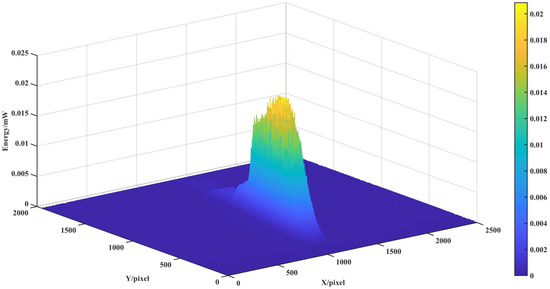
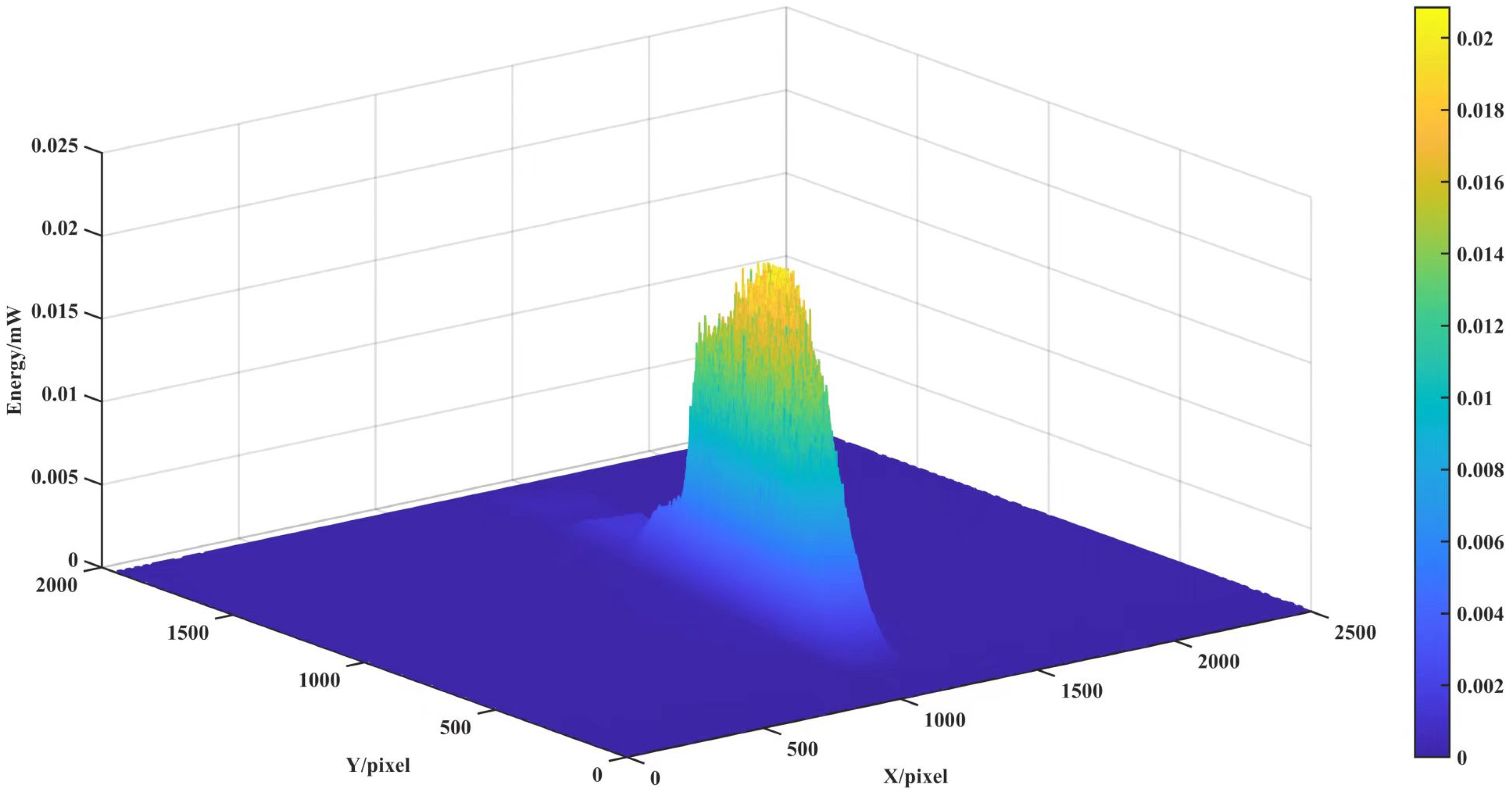
By analyzing the total grayscale values inside the aperture—the hole in the images taken while the aperture was closed—we establish a conversion between the integrated pixel sum and optical energy as detected by the calibrated photodiodes for varying exposure durations. During this process, the diffuse plate remains stationary, and only the light energy value at the opening is measured by the photodiode. We calculate the optical power incident on the system for each exposure value for which a unit grayscale intensity corresponds to each pixel. By fitting and averaging the results for several exposure values, an accurate average conversion factor can be derived to relate per-pixel grayscale intensity values to incident optical power. The power distribution for a typical spot can then be calibrated and is shown in Figure 12.

Figure 12. Spot energy distribution.

6.2. Performance Comparison

From the measurement categories we established in our previous discussions, we conducted some experimentation using several laser beams. The categories of parameters we chose to experiment on include the beam area, smallest enclosing rectangle dimension in length and width, mean luminance, max luminance, and variance of luminance in the beam area. The data from four samples of laser beams is summarized in Table 1.

Table 1. Spot measurement result.

Spot	Spot Area (mm2)	Minimum Bounding Rectangle Width (Y-Axis Direction) (mm)	Minimum Bounding Rectangle Width (X-Axis Direction) (mm)	Average Intensity	Maximum Intensity	Intensity Variance	Total Energy (mW)
Spot1	3076.42	122.45	28.47	66.04	242	64.13	6445.2
Spot2	2835.41	110.36	27.23	91.32	252	52.34	6803.5
Spot3	2553.15	90.32	30.25	85.38	215	59.68	5340.3
Spot4	2623.21	70.35	43.21	100.78	227	50.23	6402.5

Given the pronounced elliptical shape of the laser diode output beam in our experiment, we first calculated the ellipticity, defined as the ratio of the beam waist radii in the horizontal and vertical directions, which was approximately 0.231, indicating significant asymmetry. To further characterize the beam quality, we used the beam radius data measured at various propagation distances and followed the M² factor theory proposed by Siegman [35]. By fitting the beam radius evolution using the hyperbolic propagation formula,

$$\mathrm{w}(\mathrm{z})={\mathrm{w}}_0\sqrt{1+{\left({\displaystyle \frac{{\mathrm{M}}^2\mathsf{\lambda }\left(\mathrm{z}-{\mathrm{z}}_0\right)}{\mathsf{\pi }{{\mathrm{w}}_0}^2}}\right)}^2}$$

(5)

In the formula, w₀, is the waist radius, z₀ is the position of the waist on the z-axis, and M² denotes the beam quality factor. The variable z represents the distance from the laser aperture to the diffuse reflector along the beam propagation path, while $\mathrm{w}(\mathrm{z})$ is the beam radius at that point, which can be directly obtained from the data acquired by the measurement system.

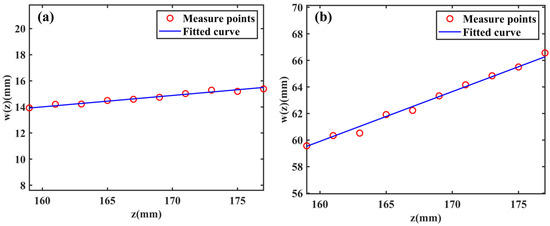
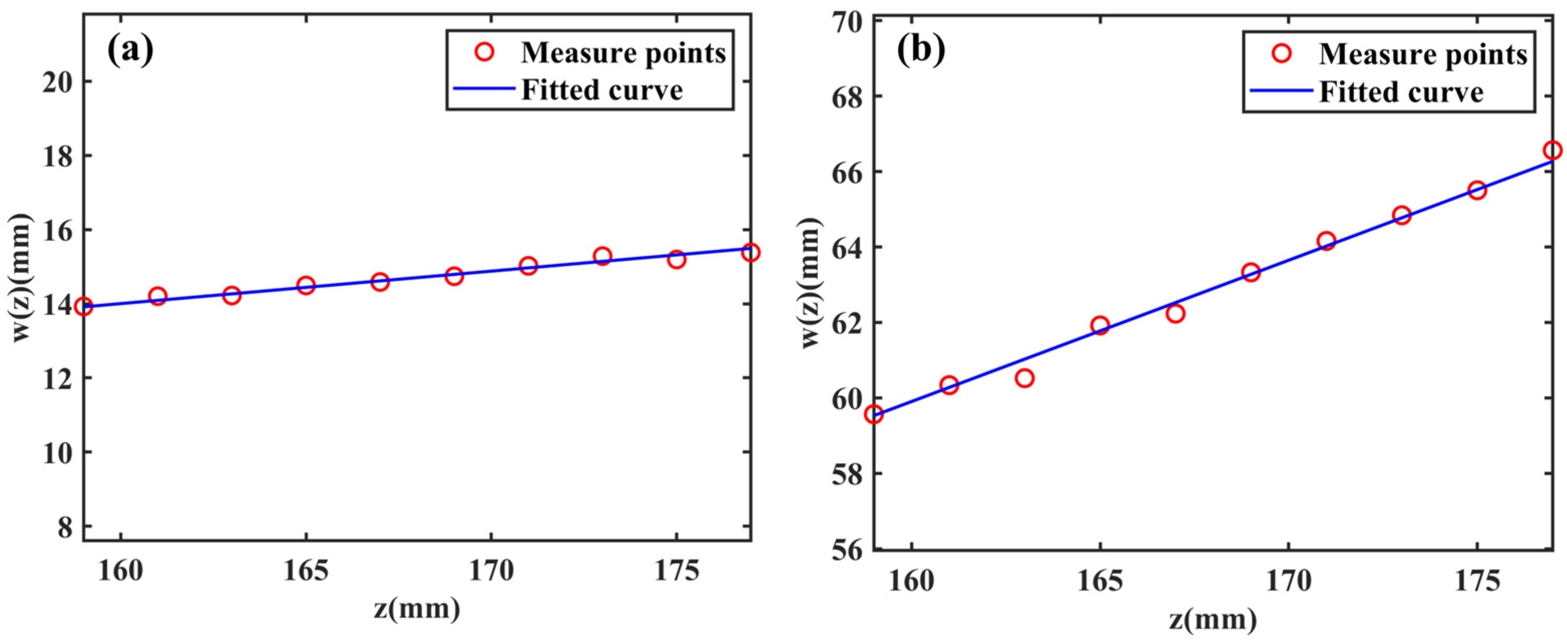
Based on the propagation equation, a set of nonlinear equations was formulated and solved under physical constraints to obtain the waist radii ${\mathrm{w}}_0$, fast ${\mathrm{w}}_0$, and slow ${\mathrm{w}}_0$; their corresponding positions ${\mathrm{z}}_0$, fast ${\mathrm{z}}_0$, and slow ${\mathrm{z}}_0$; and the corresponding M_x² and M_y² values along the fast and slow axes. The nonlinear solution was obtained by curve fitting the experimental results using the Levenberg–Marquardt method. Due to the inherently asymmetric emission characteristics of the laser diode, the beam waist was determined separately for the fast and slow axes. The experimentally obtained spot patterns are compared with the corresponding Gaussian beam patterns in Figure 13 below, where (a) represents the slow-axis direction curve and (b) represents the fast-axis direction curve.

Figure 13. Measure points and fitted curve. (a) Measured spot radii and fitted curve at different distances in the fast axis direction; (b) Measured spot radii and fitted curve at different distances in the slow axis direction.

The beam waist size of the laser diode was determined using a combination of experimental verification and theoretical calculations (the calculation is performed with the light-emitting facet of the semiconductor laser chip as the coordinate origin), and it was found to be approximately 0.39 µm for the fast axis and 1.96 µm for the slow axis. The fitting results of the experimental data yield M_x² ≈ 2.13 and M_y² ≈ 8.75, further confirming the difference in beam quality between the horizontal and vertical directions, ensuring that the accuracy of the data obtained can be used for proper optical system design.

6.3. Discussion

In this work, a flat-field correction method is introduced for CCD cameras to mitigate distortions caused by the non-uniform photoresponse of the imaging sensor during laser spot measurements. Furthermore, a spot detection algorithm based on support vector machines is presented, which enables efficient and precise localization and identification of laser spots with limited training data and computational cost. This study still has certain limitations in experimental verification and methodological completeness, which will be further explored and improved in future work.

(1)

Although a preliminary error analysis has been conducted for the system response, spot extraction and correction processes, a systematic evaluation framework has not yet been established. Specifically, quantitative indicators such as repeatability statistics, confidence interval estimation and noise tests are lacking for the random noise, systematic deviations and fitting residuals of the correction model introduced during measurement. Future work will carry out systematic error propagation analysis and uncertainty quantification to more comprehensively evaluate the reliability and repeatability of the measurement results.

(2)

The polarization characteristics of the diffuse reflector used in the experiment have not been fully verified. An ideal diffuse scatterer should be polarization-independent to ensure measurement consistency under different incident polarization states. Since the laser used in this study outputs linearly polarized light, follow-up experiments will further investigate the differences in measurement results before and after rotating the polarization direction by 90°, to clarify the influence of the polarization characteristics of the diffuse reflector on measurement accuracy and provide a basis for the system’s applicability under complex polarization conditions.

(3)

The experimental verification range of the spot intensity distribution is relatively limited. At present, only the intensity distribution under a typical spot size and single observation angle is presented, and the variation law of the spot aspect ratio under different spot sizes and incident angles has not been systematically investigated. Supplementing speckle distribution images and analyses under different geometric conditions will help to more comprehensively verify the stability of the method in diverse application scenarios.

7. Conclusions

In order to overcome the difficulties in spot measurements with high-power, wide-angle laser spots, a dedicated spot measurement system is proposed. It comprises an intensity and flat-field correction technique based on calibration of the spot measurements on a CCD detector. To address the issue of spot identification with limited computational resources, an SVM spot recognition technique is presented. It is capable of spot parameter retrieval with a high recognition accuracy of 98.11%. Before spot parameter retrieval, an intensity/shape correction technique is carried out to compensate for the system spot measurement offset due to hardware imbalance/arrangements. Various parameters of a transverse/tangential beam waist with their corresponding values are measured with a high degree of accuracy by employing a Levenberg–Marquardt algorithm. The proposed spot measurement system is capable of accurate spot measurements at high speed.

References

- Bal, A.; Palus, H. Image vignetting correction using a deformable radial polynomial model. Sensors 2023, 23, 1157. [Google Scholar] [CrossRef] [Scilit] [PubMed]
- Tian, B.; Juefei-Xu, F.; Guo, Q.; Xie, X.; Li, X.; Liu, Y. AVA: Adversarial vignetting attack against visual recognition. In Proceedings of the Thirtieth International Joint Conference on Artificial Intelligence, Montreal, QC, Canada, 21–26 August 2021. [Google Scholar]
- Liu, Y.; Long, T.; Jiao, W.; He, G.; Chen, B.; Huang, P. A general relative radiometric correction method for vignetting and chromatic aberration of multiple CCDs: Take the Chinese series of Gaofen satellite Level-0 images for example. IEEE Trans. Geosci. Remote Sens. 2022, 60, 5616725. [Google Scholar] [CrossRef] [Scilit]
- Liu, X.; Ba, D.; Jiao, D.; Shao, X.; Mu, X.; Wang, Y. Influences of analog-to-digital conversion accuracy and response uniformity of CCD on small-scale laser focal spot measurements. Laser Part. Beams 2021, 2021, e20. [Google Scholar] [CrossRef] [Scilit]
- Fossum, E.R.; Hondongwa, D.B. A review of the pinned photodiode for CCD and CMOS image sensors. IEEE J. Electron Devices Soc. 2014, 2, 33–43. [Google Scholar] [CrossRef] [Scilit]
- Li, J.; Wang, J.; Zhou, B.; Shen, W. Nonuniformity correction and calibration method in the high-precision CCD measurement and servo control system. In Proceedings of the 48th IEEE Conference on Decision and Control, CDC 2009, Combined with the 28th Chinese Control Conference, Shanghai, China, 15 December 2009. [Google Scholar]
- Zhou, F.; Cui, Y.; Liu, L.; Gao, H. Distortion correction using a single image based on projective invariability and separate model. Opt. Int. J. Light Electron Opt. 2013, 124, 3125–3130. [Google Scholar] [CrossRef] [Scilit]
- Kukko, A.; Kaasalainen, S.; Litkey, P. Effect of incidence angle on laser scanner intensity and surface data. Appl. Opt. 2008, 47, 986–992. [Google Scholar] [CrossRef] [Scilit] [PubMed]
- Bal, A.; Palus, H. A smooth non-iterative local polynomial (SNILP) model of image vignetting. Sensors 2021, 21, 7086. [Google Scholar] [CrossRef] [Scilit] [PubMed]
- Goldman, D.B. Vignette and exposure calibration and compensation. IEEE Trans. Pattern Anal. Mach. Intell. 2010, 32, 2276–2288. [Google Scholar] [CrossRef] [Scilit]
- Lee, J. Offset and Gain FPN Calibrated Linear-Logarithmic Image Sensor With Shared Pixel Architecture. IEEE Trans. Circuits Syst. II Express Briefs 2021, 68, 3518–3521. [Google Scholar] [CrossRef] [Scilit]
- Fossum, E.R.; Teranishi, N.; Theuwissen, A.J. Digital image sensor evolution and new frontiers. Annu. Rev. Vis. Sci. 2024, 10, 171–198. [Google Scholar] [CrossRef] [Scilit]
- Li, J.; Su, J.; Zeng, X. A solution method for image distortion correction model based on bilinear interpolation. Comput. Opt. 2019, 43, 99–104. [Google Scholar] [CrossRef] [Scilit]
- Ye, Y.; Xia, M.; Kong, D.; Zhai, W.; Xu, M.; Ge, P.; Zhou, A.; Zheng, X. Study of 256 fiber array biaxial LiDAR optical assembly measurements. Opt. Express 2023, 31, 27136–27146. [Google Scholar] [CrossRef] [Scilit] [PubMed]
- Ke, Y.; Zeng, C.; Xie, P.; Jiang, Q.; Liang, K.; Yang, Z.; Zhao, M. Measurement system with high accuracy for laser beam quality. Appl. Opt. 2015, 54, 4876–4880. [Google Scholar] [CrossRef] [Scilit] [PubMed]
- Zhao, Y.; Xiao, Z.; Liang, X.; Bao, L. Study of zero position variation for an optical sight by using a CCD. J. Opt. Technol. 2019, 86, 374–378. [Google Scholar] [CrossRef] [Scilit]
- He, X.; Pan, X.; Tao, H.; Liu, C.; Zhu, J. Single-shot measurement of the near-field and focal spot profiles of a 351 nm laser beam for SGII-upgraded facility with multiple-focal-plane constraint coherent modulation imaging. Opt. Express 2022, 30, 42861–42874. [Google Scholar] [CrossRef] [Scilit]
- Abdo, M.; Badilita, V.; Korvink, J. Spatial scanning hyperspectral imaging combining a rotating slit with a Dove prism. Opt. Express 2019, 27, 20290–20304. [Google Scholar] [CrossRef] [Scilit]
- Li, S.; Chen, Z.; Xie, L.; Liao, Q.; Zhou, X.; Chen, Y.; Lin, X. Weak measurements of the waist of an arbitrarily polarized beam via in-plane spin splitting. Opt. Express 2021, 29, 8777–8785. [Google Scholar] [CrossRef] [Scilit]
- Luo, J.; Qin, L.; Hou, Z.; Zhang, S.; Zhu, W.; Guan, W. Study on laser parameter measurement system based on cone-arranged fibers and CCD camera. Sensors 2022, 22, 7892. [Google Scholar] [CrossRef] [Scilit] [PubMed]
- Miao, C.; Xiao, W.; Qinghua, Y. Influence analysis of laser spot noise on the measurement accuracy of laser triangulation method. Int. J. u- e-Serv. Sci. Technol. 2016, 9, 39–46. [Google Scholar] [CrossRef] [Scilit]
- Nan, Z.; Feng, Y.; Zhao, H.; Tao, W. Research on laser source drift with temperature of laser triangular displacement sensor. In Proceedings of the Ninth International Symposium on Precision Mechanical Measurements, Chongqing, China, 18 October 2019. [Google Scholar]
- Zhou, X.; Wang, J.; Liang, X.; Xiao, Y.; Liu, J. Application of an image fusion algorithm in measuring the laser beam far-field divergence angle. J. Opt. Technol. 2018, 85, 148–152. [Google Scholar] [CrossRef] [Scilit]
- Ji, K.-H.; Hou, T.-R.; Li, J.-B.; Meng, L.-Q.; Han, Z.-G.; Zhu, R.-H. Fast measurement of the laser beam quality factor based on phase retrieval with a liquid lens. Appl. Opt. 2019, 58, 2765–2772. [Google Scholar] [CrossRef] [Scilit] [PubMed]
- Xie, J.; Chen, H.; Tan, Z.; Hou, D.; Wang, X. Novel measurement method of infrared laser beam divergence angle based on two linear array CCDs. In Proceedings of the International Symposium on Photoelectronic Detection and Imaging 2013: Infrared Imaging and Applications, Beijing, China, 25 June 2013. [Google Scholar]
- Pan, S.; Ma, J.; Zhu, R.; Ba, T.; Zuo, C.; Chen, F.; Dou, J.; Wei, C.; Zhou, W. Real-time complex amplitude reconstruction method for beam quality M2 factor measurement. Opt. Express 2017, 25, 20142–20155. [Google Scholar] [CrossRef] [Scilit]
- Meng, F.; Yang, G.; Yang, J.; Lu, H.; Dong, Z.; Kang, R.; Guo, D.; Qin, Y. Error analysis of normal surface measurements based on multiple laser displacement sensors. Sensors 2024, 24, 2059. [Google Scholar] [CrossRef] [Scilit]
- Zhang, W.; Guo, W.; Zhang, C.; Zhao, S. An improved method for spot position detection of a laser tracking and positioning system based on a four-quadrant detector. Sensors 2019, 19, 4722. [Google Scholar] [CrossRef] [Scilit] [PubMed]
- Nan, Z.; Zhou, L.; Wan, S.; Wang, Y.; Tao, W. Research on laser spot location accuracy of low-power laser diode source applied to high precision laser measurement system. Meas. Sci. Technol. 2022, 34, 015124. [Google Scholar] [CrossRef] [Scilit]
- Kudryashov, A.V.; Rukosuev, A.; Kopylov, E.; Samarkin, V.; Galaktionov, I. Fast adaptive optical system for 1.5 km horizontal beam propagation. Proc. SPIE 2018, 10772, 250–258. [Google Scholar] [CrossRef] [Scilit]
- Li, X.; Wang, A.; Fan, M.; Yu, L.; Liang, X. Multi-Spectral and Single-Shot Wavefront Detection Technique Based on Neural Networks. Photonics 2025, 12, 1110. [Google Scholar] [CrossRef] [Scilit]
- Xia, A.-L.; Ma, C.-W. An improved centroid detection method based on higher moment for Shack-Hartmann wavefront sensor. Proc. SPIE 2010, 7850, 356–361. [Google Scholar] [CrossRef] [Scilit]
- Chen, N.; Zhang, J.; Zhong, S.; Mao, W.; Hu, D.; Yao, L. Two-dimensional calibration for fixed-pattern noise reduction of thermal images. In Proceedings of the 2019 IEEE International Symposium on Circuits and Systems (ISCAS), Sapporo, Japan, 26 May 2019. [Google Scholar]
- Patil, P.V.; Patil, N.C. Survey on Otsu Image Segmentation Algorithm. Int. J. Sci. Dev. Res. 2016, 1, 4. Available online: https://openrgate.org/viewfulldetails.php?id=5592 (accessed on 26 February 2026).
- Siegman, A.E. New developments in laser resonators. In Optical Resonators; SPIE: Bellingham, WA, USA, 1990; Volume 1224, pp. 2–14. [Google Scholar]
Disclaimer/Publisher’s Note: The statements, opinions and data contained in all publications are solely those of the individual author(s) and contributor(s) and not of MDPI and/or the editor(s). MDPI and/or the editor(s) disclaim responsibility for any injury to people or property resulting from any ideas, methods, instructions or products referred to in the content. |
© 2026 by the authors. Licensee MDPI, Basel, Switzerland. This article is an open access article distributed under the terms and conditions of the Creative Commons Attribution (CC BY) license.