


Abstract
Background: Transcranial magnetic stimulation (TMS) enables functional brain mapping by linking stimulation (electric field) to motor evoked responses (MEPs), but accurate mapping often requires many empirical samples. Prediction models based only on TMS setup parameters have limited ability to account for subject-specific anatomy, whereas 3D intracranial E-Fields provide richer biophysical information but may suffer from sparse volumetric representations. This study aimed to predict MEPs from individualized cortical E-Field distributions using flattened two-dimensional cortical maps. Methods: TMS–MEP experiments were conducted in seven healthy participants. MRI-derived head models were used to simulate FEM-based intracranial E-Fields for each stimulation condition. Primary motor cortex E-Fields were transformed into two-dimensional cortical maps, and multiple deep learning models were evaluated using nested cross-validation with held-out-subject testing with subject-wise inner validation (HOS-SIV) as a stricter setting and held-out-subject testing with random inner validation (HOS-RIV). Results: ROC-AUC values ranged from 0.710 to 0.811 and from 0.840 to 0.872 across muscles under the held-out-subject testing with subject-wise inner validation (HOS-SIV) and held-out-subject testing with random inner validation (HOS-RIV) settings, respectively. Under the primary HOS-SIV setting, conventional classifiers and CNN-based models showed broadly comparable performance, whereas CNN- and ResNet-based models tended to perform better under the HOS-RIV setting. Predicted spatial MEP maps partially reproduced the measured response distributions. Conclusions: The presence of TMS-induced MEPs can be predicted from flattened maps of subject-specific cortical E-fields, providing proof-of-concept support for future approaches to improve the efficiency of TMS motor mapping.
1. Introduction
Transcranial magnetic stimulation (TMS) is a noninvasive brain stimulation technique that induces an electric field (E-field) in the brain according to Faraday’s law [1]. When applied to the motor cortex, TMS activates cortical neurons, and this activity propagates through the corticospinal tract to evoke motor evoked potentials (MEPs) in target muscles [2]. The cortical site at which MEPs are most readily elicited is referred to as the hotspot [3], and identifying this site is fundamental for functional brain mapping [4]. For example, TMS-based functional mapping has been reported to support preoperative mapping with navigated TMS, improving both surgical safety and efficacy [5].
It has become increasingly evident that TMS-based mapping cannot rely solely on external stimulation parameters, such as position and orientation of the TMS coil, because participant-specific anatomical and electrical factors also shape the cortical E-field. These include scalp-to-cortex distance [6,7], cortical geometry, cerebrospinal fluid volume, and tissue electrical properties [8,9]. These factors affect the spatial distribution and magnitude of the E-field reaching the cortex. Consequently, the same external stimulation parameters may induce different cortical E-field patterns across individuals, making it difficult to predict the cortical site and stimulation conditions that elicit MEPs. To account for these effects, numerical modeling of the TMS-induced E-field has emerged as an important approach. Typically, subject-specific head models are reconstructed from MRI data, and computational methods, such as the finite element method (FEM), are used to simulate the distribution and strength of the induced E-field within the brain [10]. However, although FEM-based modeling provides a subject-specific estimate of the neural dose, predicting whether a given E-field distribution will elicit an MEP remains challenging because the relationship between cortical field patterns and corticospinal output is nonlinear and non-trivial [11]. In conventional TMS-based motor mapping, this relationship is usually characterized by sampling across multiple coil positions, orientations, stimulation intensities, and target muscles [12,13]. Such sampling can improve the reliability of individualized motor maps, but it also prolongs experimental sessions and increases participant or patient burden, and recent approaches have sought to reduce this burden [14]. If MEP responses can be predicted from subject-specific stimulation information, the time required for motor mapping procedures may be reduced.
Predictions of MEP occurrence have been made using conventional machine learning models based on TMS setup parameters, including coil position, coil orientation, and stimulation intensity [15]. Although encouraging results were obtained within subjects, results between subjects decreased substantially, suggesting limited generalizability across individuals. One possible reason is that the stimulation parameters alone do not explicitly represent the subject-specific intracranial E-field shaped by individual anatomy, as mentioned earlier, and they provide only an indirect description of the neural dose. To date, only one group combined FEM-based E-field simulation with a deep neural network to predict multi-muscle responses [16], and this framework was later extended to estimate the intracranial E-field from MEPs as an inverse problem [17]. However, because these approaches relied on three-dimensional volumetric E-field inputs, dimensionality reduction with an autoencoder was required, resulting in a two-stage learning process. Such a design increases model complexity and may reduce practicality for efficient motor mapping. In addition, when the 3D E-field is represented only within the cortical mask, where activation occurs, the resulting input becomes highly sparse, with many zero-valued voxels. Such sparsity may reduce learning efficiency and limit the model’s ability to capture broader cortical field patterns relevant to MEP generation.
Although three-dimensional E-field volumes preserve anatomical detail, they contain substantial information that is weakly relevant to motor mapping, particularly outside the cortical regions most directly involved in MEP generation. A cortical flat-map representation offers a more targeted alternative by projecting the subject-specific E-field onto the cortical sheet and expressing it as a compact two-dimensional map [18]. This approach reduces irrelevant volumetric information while retaining the spatial organization of the cortical field pattern relevant to MEP generation. To the best of our knowledge, no previous deep learning study has directly used TMS-induced cortical E-fields represented as two-dimensional flat maps for MEP prediction.
In this study, we aimed to determine whether TMS-induced MEPs could be predicted from cortical E-field distributions while reducing the dependence of motor mapping on extensive empirical sampling. To achieve this, we collected TMS–MEP data from seven participants and generated individualized three-dimensional E-field distributions based on MRI-derived head models. Then, a flattened, two-dimensional representation of a three-dimensional cortical E-field distribution was used as a computationally efficient alternative to the original three-dimensional input. We then trained different models to predict MEPs from these simulated fields. Finally, nested cross-validation was employed to evaluate the generalization performance of the proposed approach on unseen subjects.
2. Methods
2.1. Data Acquisition
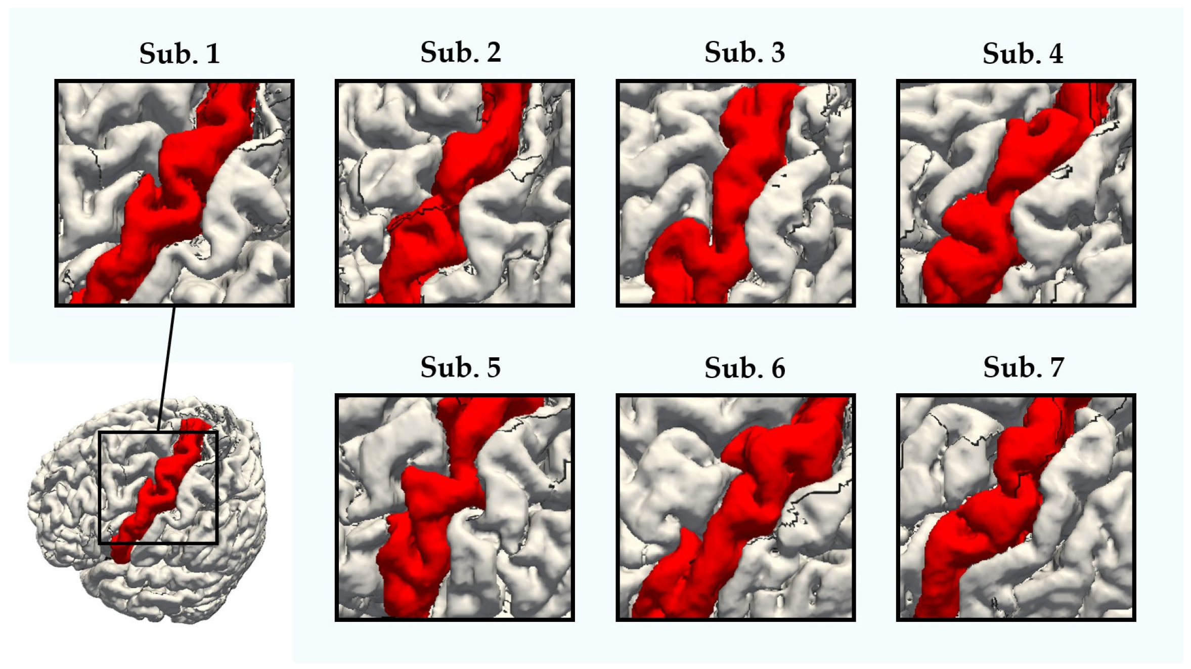
Seven healthy volunteers participated in the study (mean age, 22 ± 1.5 years; 6 males and 1 female). Written informed consent was obtained from all participants before participation. For each participant, a T1-weighted MRI scan (MP-RAGE; TR = 2400 ms, TE = 2.24 ms, TI = 1060 ms, flip angle = 8°, field of view = 240 × 256 mm2, matrix size = 300 × 320, voxel size = 0.8 × 0.8 × 0.8 mm3) and T2-weighted MRI scan (3D-SPACE; TR = 3200 ms, TE = 560 ms, flip angle = 120°, FOV = 240 × 256, matrix = 302 × 320, voxel size = 0.8 × 0.8 × 0.8 mm3) were acquired on 3T scanner (Magnetom Verio, Siemens Healthineer, Erlangen, Germany) prior to the experiments. It was confirmed that the subjects showed distinct gyrification patterns in the primary motor area (Appendix A), even within a relatively homogeneous cohort.
On a separate day, TMS experiments were conducted to measure the MEP under different stimulation conditions. Stimulation was delivered using a Magstim Rapid2 stimulator (The Magstim Company Ltd., Whitland, UK) with a 70 mm Double AirFilm coil. The position and orientation of the coil relative to the participant’s head were continuously monitored using Brainsight TMS neuronavigation software (Rogue Research Inc., Montreal, QC, Canada, version 2.4.11).
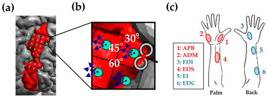
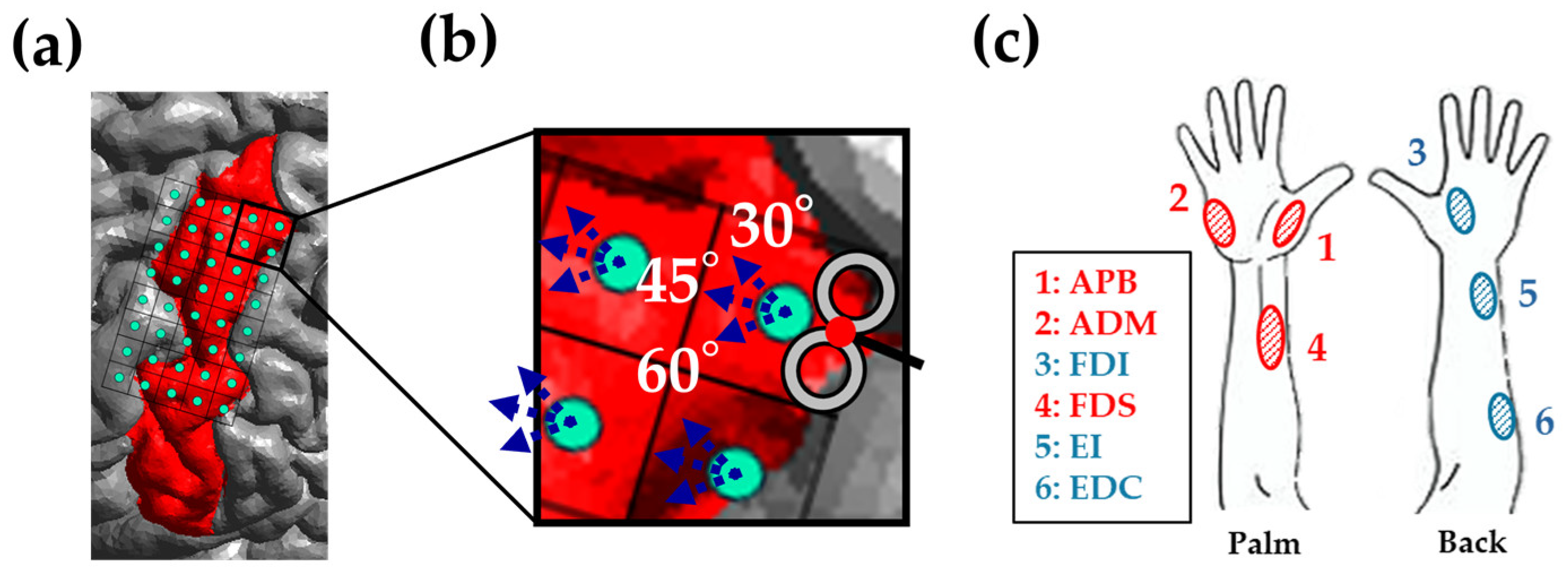
For coil placement, an 8 × 5 grid with 5 mm spacing was defined on the gray matter surface of the primary motor cortex, centered on the previously identified hotspot of the abductor pollicis brevis (APB) (Figure 1a). Coil orientation varied relative to the direction parallel to the interhemispheric fissure, with three angles tested: 30°, 45°, and 60° (Figure 1b). Stimulation intensity was then applied at 100% and 120% of the motor threshold. The stimulation parameters were selected to produce non-identical changes in the induced E-field in the brain and MEPs [7,19].
Figure 1.
Experimental setup for TMS and MEP recordings. (a) A stimulation grid (8 × 5) with 5 mm spacing was defined over the cortical surface, and the TMS coil was positioned at each grid point; (b) Coil orientation was varied relative to the sagittal plane, with three angles (30°, 45°, and 60°), while maintaining the coil perpendicular to the cortical surface; (c) Target muscles for MEP recording on the right arm. On the palmar side: APB, ADM, and FDS; on the dorsal side: FDI, EI, and EDC. Red color indicates the primary motor cortex.
MEPs were recorded using an evoked potential/electromyography system (Neuropack MEB-2200, Nihon Kohden, Tokyo, Japan) and disposable foam surface electrodes (130 Foam ECG electrodes, Cardinal Health). Each MEP signal was denoised by removing TMS-pulsed-dominated frequency components. Recordings were obtained from six muscles in the right hand and forearm: the abductor pollicis brevis (APB), abductor digiti minimi (ADM), first dorsal interosseous (FDI), flexor digitorum superficialis (FDS), extensor indicis (EI), and extensor digitorum communis (EDC) (Figure 1c). Resting motor threshold (RMT) was measured at the APB hotspot, defined as the minimum intensity required to evoke MEPs with a peak-to-peak amplitude of at least 50 μV in at least 5 out of 10 trials [20,21].
For each combination of coil position, orientation, and intensity, MEPs were recorded five times per muscle with inter-stimulus intervals of approximately 5 s. Peak-to-peak amplitudes were extracted and averaged for 5 repetitions within each trial. Because MEP responses typically exhibit substantial trial-to-trial variability, averaging five repetitions improves the reliability of the MEP amplitude estimate [22], while providing a practical compromise with experimental duration. In total, 7200 MEP measurements were obtained per participant (40 coil positions × 3 coil angles × 2 intensities × 6 muscles × 5 repetitions). After averaging across repetitions, the dataset comprised 240 mean peak-to-peak MEP amplitudes per muscle for each participant (40 coil positions × 3 coil angles × 2 intensities).
2.2. Numerical Modeling
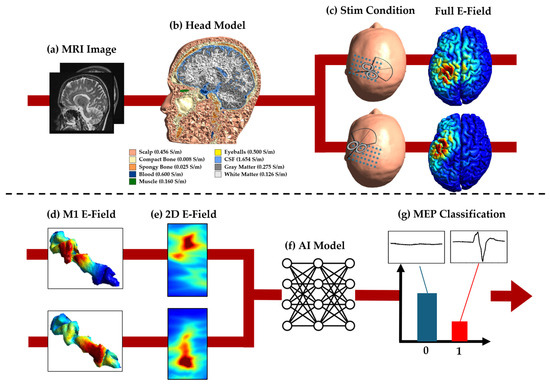
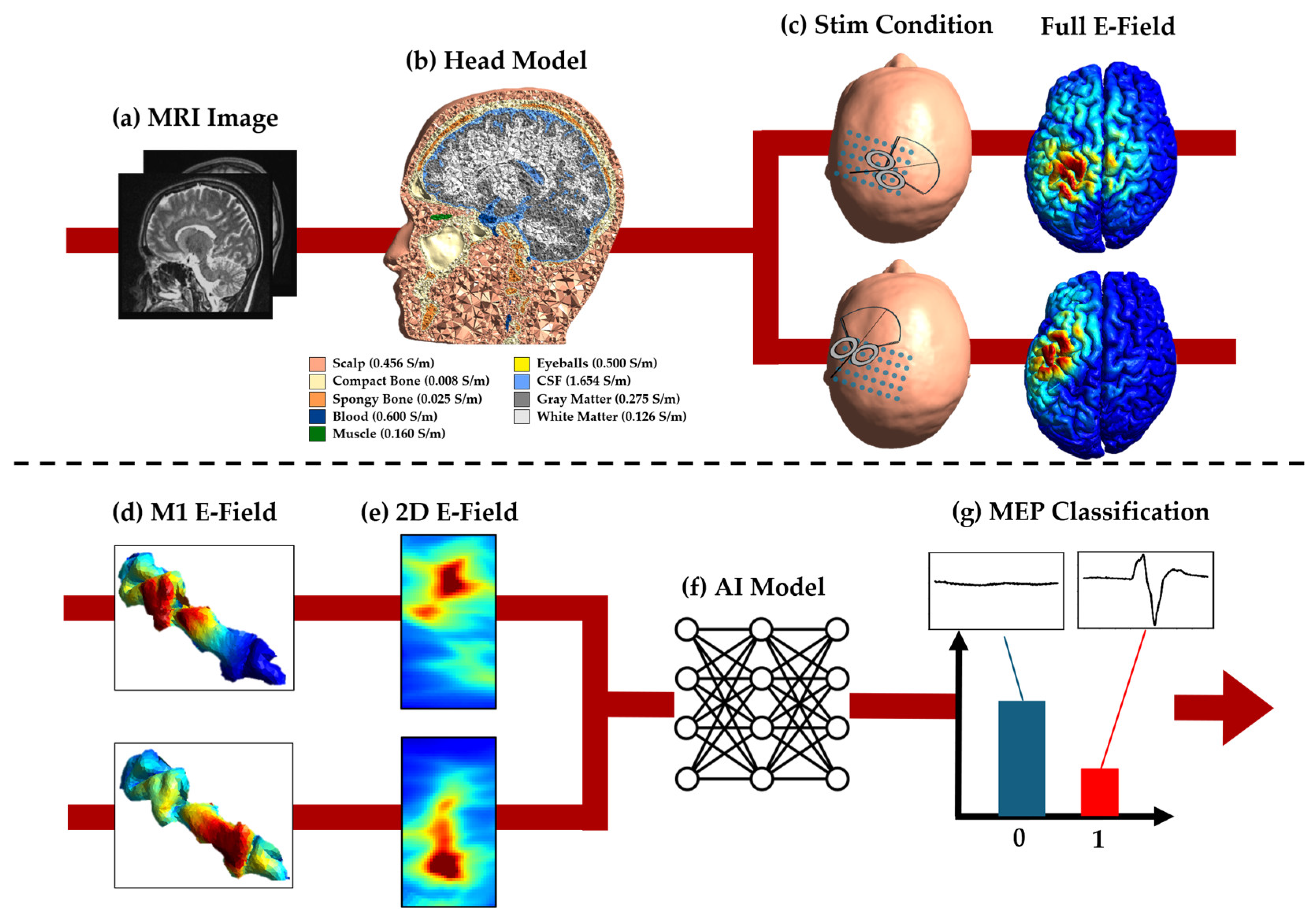
Figure 2a–c show the use of individualized head models. A head model for each participant was constructed from structural MRI data using the charm pipeline available in SimNIBS (version 4.0) [23]. The electrical conductivity values, (S/m), assigned to each segmented tissue were as follows: white matter ( = 0.126), gray matter ( = 0.275), cerebrospinal fluid ( = 1.654), scalp ( = 0.465), eyeballs ( = 0.500), compact bone ( = 0.008), spongy bone ( = 0.025), blood ( = 0.600), and muscle ( = 0.160) [24,25,26]. For each stimulation condition, an individualized, induced E-field was computed in a numerical FEM solver (SimNIBS) under the quasi-static approximation. The scalar electric potential was obtained by
and the E-field was calculated as
Figure 2.
Workflow for predicting MEP presence using MRI-based E-field simulations. (a) T1- and T2-weighted MRI scans were obtained from each of the seven participants; (b) Individualized head models were generated using the charm command in SimNIBS 4.0; (c) E-field distributions were simulated in SimNIBS for each averaged peak-to-peak MEP sample; (d,e) The E-field in the primary motor cortex was extracted from the whole-brain and unfolded into a 2D grid using the Cgrid toolbox; (f) MEP presence was predicted from the 2D E-field maps using multiple deep learning models; (g) Binary labeling of MEP presence based on peak-to-peak amplitude (≥50 μV = 1, <50 μV = 0).
The magnetic vector potential was derived from a coil model generated using Kodein Box (version 1.0), a tool for constructing user-defined TMS coil geometries from conductor path data [27]. The coil model was configured to match the one used in the experiment, consisting of 12 turns, each with an inner diameter of 21 mm and an outer diameter of 105 mm.
2.3. E-Field and MEP Preprocessing
MEP generation is primarily driven by neuronal activation in cortical regions. Therefore, large portions of the intracranial E-field volume are not directly relevant [28,29]. Moreover, using full volumetric data as input to the deep learning model would substantially increase dimensionality and computational cost.
To obtain a compact, functionally relevant representation, the region of interest was flattened (see Figure 2d,e). The brain was first parcellated using FreeSurfer (Ver. 6.0), and the region of interest (the primary motor cortex) was identified [30]. The open-source Cgrid-toolbox was then used to perform a geometry-preserving flattening of the curved cortical patch and resample it onto a regular 2D Cartesian grid (60 × 40 × 1 representation) [31]. This flattened representation preserves cortical topology and spatial relationships, including both gyral crowns and sulcal banks relevant for MEP generation [32]. The resulting two-dimensional E-field maps were used as inputs to the deep learning model (Figure 2f). The averaged peak-to-peak MEPs were binarized at 50 μV (≥50 μV: 1; <50 μV: 0) in Figure 2g, following the criterion for resting motor threshold [20,21].
2.4. Model Training and Evaluation
Before model training, the E-field maps were standardized using z-score normalization based on the training participants in each outer fold. The held-out test participant was excluded when calculating the mean and standard deviation.
Three CNN-based models and four ResNet-based models were used for classification, as summarized in Table 1. The CNN-based models were used to examine the effects of different network depths and channel dimensions on classification performance. The ResNet-based models were used to evaluate the effects of residual connections, channel width, and residual block configuration. The input to the model was a two-dimensional E-field map of size 60 × 40 × 1 per stimulation condition. We trained a separate binary classification model for each muscle to predict the presence of an MEP.
Table 1.
Summary of model architectures and configurations.
CNN-based models
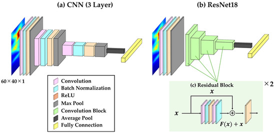
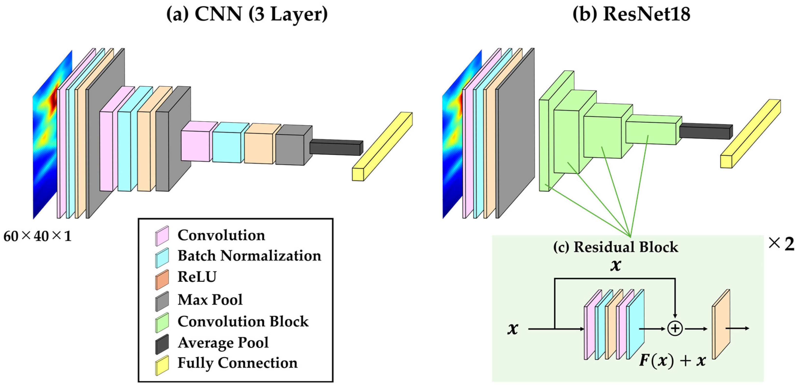
Three CNN-based models were used: CNN2Layer, CNN3Layer, and CNN4Layer. All models consist of stacked convolutional blocks, adaptive average pooling, and a fully connected output layer. Each convolutional block includes a 3 × 3 convolution with stride 1 and padding 1, batch normalization [33], ReLU activation, and 2 × 2 max pooling. The channel dimensions were [32, 64], [32, 64, 128], and [32, 64, 128, 256] for CNN2Layer, CNN3Layer, and CNN4Layer, respectively. The extracted feature maps were then aggregated into a 1 × 1 representation using adaptive average pooling and passed to a fully connected layer with one output unit. The architecture of CNN3Layer, used as a representative CNN-based model, is shown in Figure 3a.
Figure 3.
Architectures of the CNN-based and ResNet-based models used in this study. (a) CNN-based architecture composed of stacked convolutional blocks; (b) ResNet-based architecture composed of residual blocks; (c) Residual Block structure used in the ResNet-based models, where the input is added to the residual mapping via a shortcut connection.
ResNet-based models
Four ResNet-based models were used: ResNet18, ResNet18SmallInput, ResNet18Lite, and ResNetTiny. ResNet18 [34] was used as a standard model (Figure 3b). It is based on residual blocks, in which the input feature map is added to the output of the convolutional layers via a shortcut connection. In this model, each stage contains two residual blocks, resulting in a block configuration of [2, 2, 2, 2]; the residual block structure is shown in Figure 3c. ResNet18SmallInput is a modified version of the standard ResNet18, designed to account for the small spatial size of the input images. The initial convolutional layer is replaced with a 3 × 3 convolution with a stride of 1 and padding of 1, and the max pooling layer is removed to reduce excessive early-stage downsampling. The residual block configuration remains the same as in ResNet18, with channel dimensions of 64, 128, 256, and 512. ResNet18Lite is also designed for small input images. Similar to ResNet18SmallInput, it uses a 3 × 3 initial convolution, with a stride of 1 and a padding of 1, and does not use max pooling. The number of residual blocks is kept as [2, 2, 2, 2], preserving the depth of ResNet18. However, the initial number of channels is reduced to 32, resulting in stage-wise channel dimensions of 32, 64, 128, and 256. Therefore, ResNet18Lite maintains the same residual block depth as ResNet18SmallInput while reducing the number of parameters by narrowing the channel width. ResNetTiny is the most compact ResNet-based model used in this study. Like ResNet18Lite, it uses a 3 × 3 initial convolution with stride 1 and padding 1, without max pooling, to preserve spatial information for small input images. In addition, the number of residual blocks is reduced to one per stage, resulting in a block configuration of [1, 1, 1, 1]. The initial number of channels is set to 16, and the channel dimensions of the four stages are 16, 32, 64, and 128. As a result, ResNetTiny preserves the residual learning structure while reducing both the network depth and channel width.
Model Training and Evaluation for CNN- and ResNet-Based Models
Binary cross-entropy (BCE) was used as the loss function. Model parameters were optimized using AdamW [35] with a weight decay of 0.001. For hyperparameter tuning, we performed a random search over the learning rate by sampling 40 values on a logarithmic scale between 0.0004 and 0.04. Training was performed for up to 100 epochs with a batch size of 64, and early stopping with a patience of 5 epochs was applied to reduce overfitting (Appendix B). Classification performance was assessed separately for each muscle using ROC-AUC and PR-AUC.
All models were implemented in PyTorch 2.9.1 and trained on a workstation equipped with an Intel Xeon w3-2435 CPU (8 cores, 3.1 GHz), an NVIDIA RTX 4000 SFF Ada GPU (20 GB), and 64 GB RAM.
Machine-Learning Classifiers
To evaluate whether convolutional architectures provided advantages over simpler classifiers, performance was compared with conventional machine-learning classifiers. Specifically, logistic regression and linear support vector machine (SVM) were used as baseline models. Unlike the CNN model, these classifiers do not explicitly learn local spatial features from the two-dimensional E-field maps. Therefore, this comparison was conducted to examine whether the spatial feature extraction capability of CNNs contributes to improved MEP prediction performance. Model performance was evaluated using nested cross-validation, ensuring that hyperparameter tuning was performed only within the training data of each outer fold. The regularization parameter was optimized by grid search. For both logistic regression and linear SVM, the candidate values of were set to 0.01, 0.1, 1, 10, and 100. Logistic regression was implemented with the liblinear solver, and the linear SVM with LinearSVC. Balanced class weights were used for both classifiers to account for class imbalance. The E-field input maps were flattened into one-dimensional feature vectors before being provided to the conventional classifiers. This preprocessing was required because logistic regression and linear SVM operate on vectorized feature representations rather than two-dimensional image-like inputs. The resulting classification performance was then compared with that of the deep learning models using the same evaluation metrics.
2.5. Data Splitting and Validation Procedure
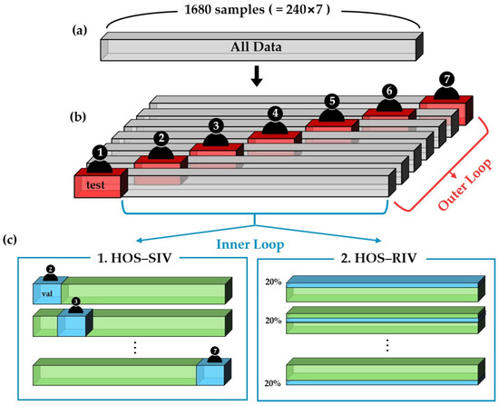
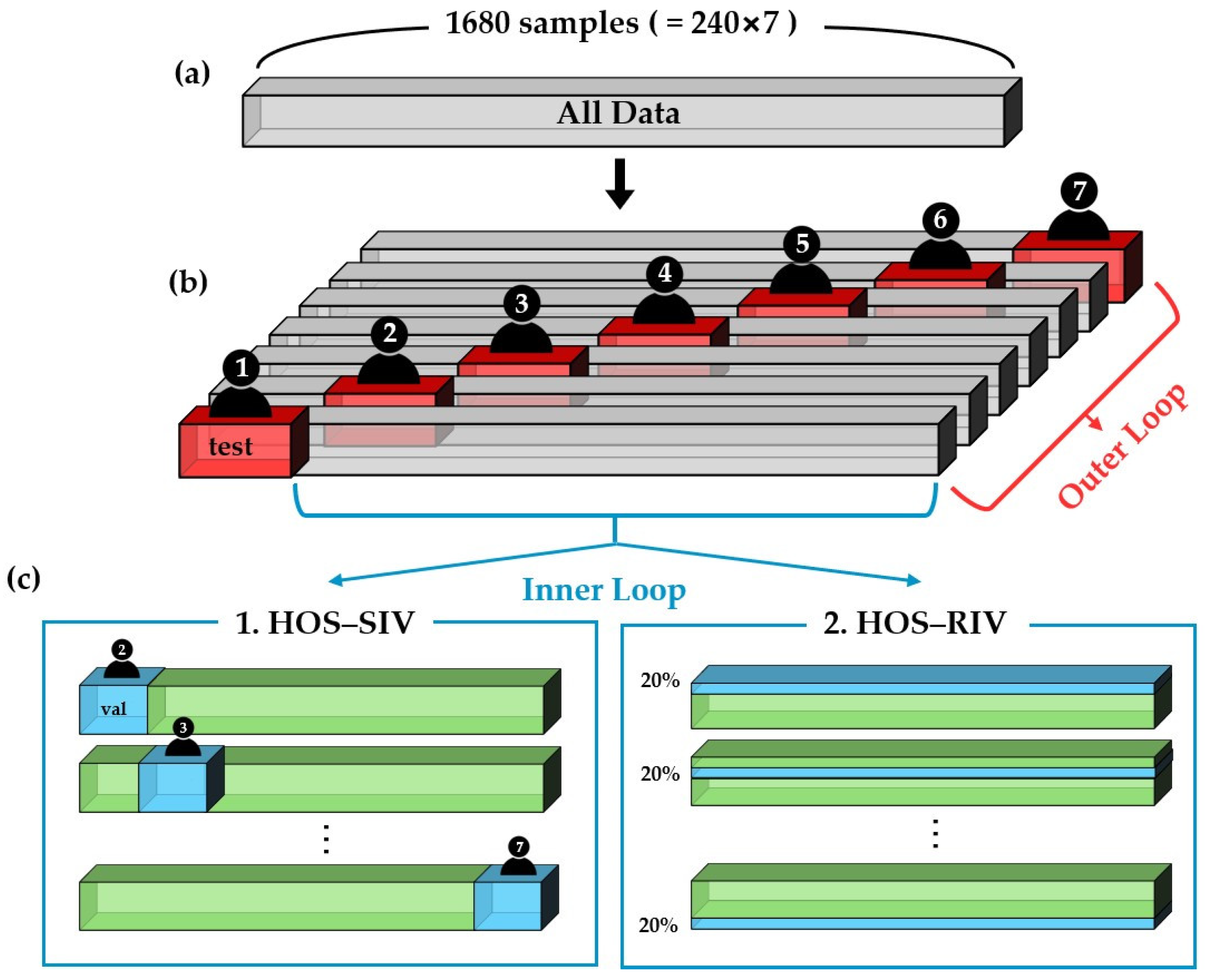
As shown in Figure 4, to properly evaluate predictive performance on unseen subjects, nested cross-validation [36] was adopted as the data-splitting strategy. In the outer loop, one participant was held out as the test set, and the remaining participants were used to develop the model. This subject-wise outer separation was used to prevent data leakage across subjects. In the inner loop, two validation strategies were examined. We refer to these two settings as held-out-subject testing with subject-wise inner validation (HOS-SIV) and held-out-subject testing with random inner validation (HOS-RIV). In the HOS-SIV setting, one participant from the outer training set was used as the validation subject. Therefore, both the inner validation subject and the outer test subject were unseen during their respective training stages. This was regarded as the primary analysis, as this strategy provides the most conservative assessment of subject-level generalization during model selection. In the HOS-RIV setting, the inner-training and inner-validation samples share participant-specific characteristics; the outer test subject remained completely excluded in all cases. Here, 20% of the pooled samples from the outer training participants were randomly assigned to the validation set. This setting was evaluated as a secondary analysis to assess performance when validation data were drawn from the same participant pool as the training data.
Figure 4.
Overview of the nested cross-validation procedure. (a) The full dataset consisted of 240 simulations per participant’s muscle (40 coil positions × 3 coil angles × 2 intensities) in 7 participants; (b) In the outer loop, subject-wise splitting was performed, with one participant held out as the test set in each fold; (c) In the inner loop, two validation strategies were examined for hyperparameter selection: (1) in the HOS-SIV setting, one participant from the training set was used for validation, and (2) in the HOS-RIV setting, 20% of the pooled training samples were randomly assigned to the validation set.
In each inner fold, the hyperparameter set yielding the lowest validation loss was selected. The same outer folds and the same train/test splits were used for the ResNet, CNN, and conventional machine-learning methods.
3. Results
3.1. Distribution of Experimental MEP Responses
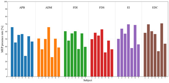
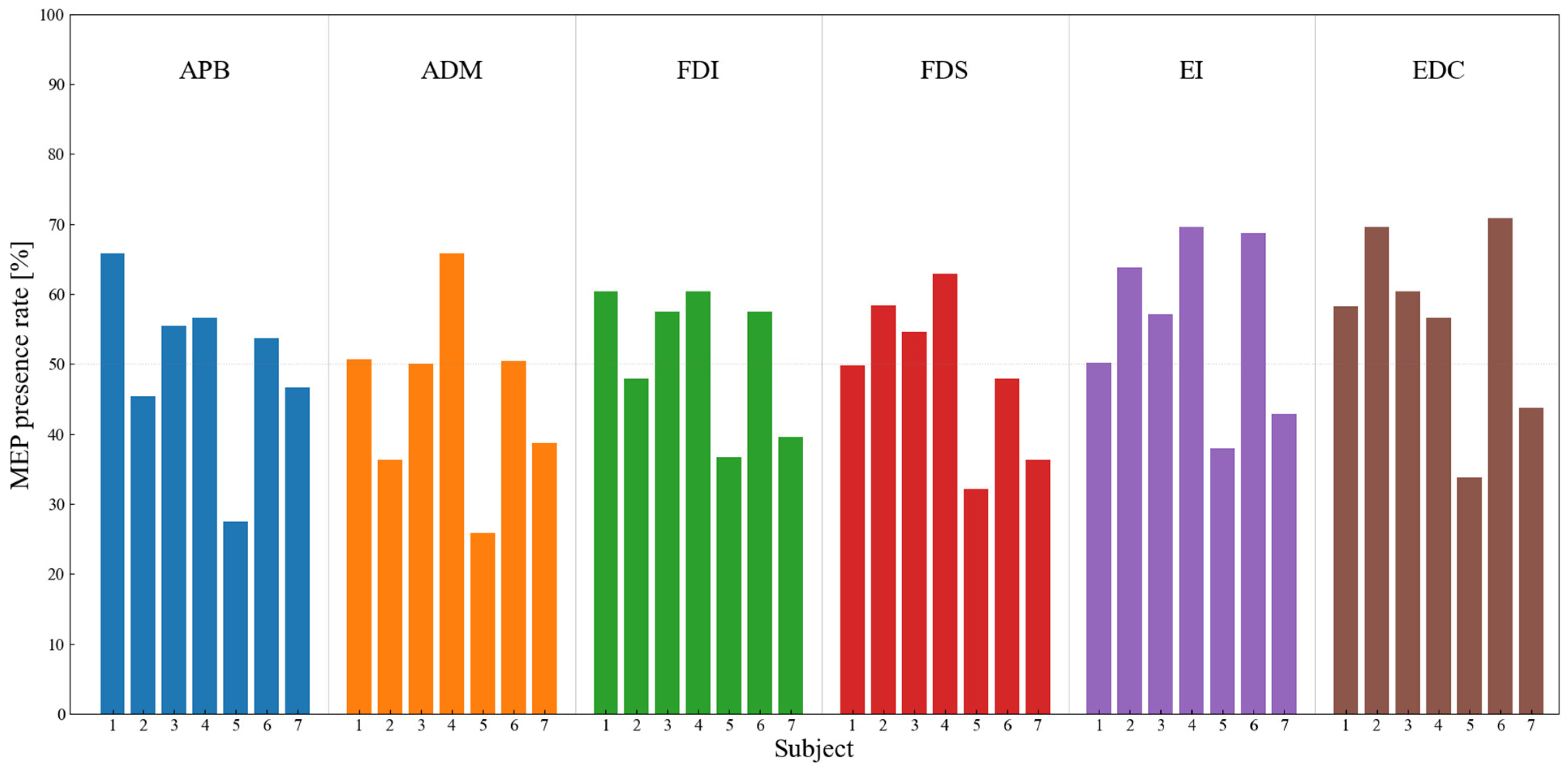
Figure 5 shows the portion of stimulation samples that elicited MEP-positive responses for each participant and each target muscle. Variability was observed both across participants and within participants across muscles. Among the seven participants, participant 5 exhibited the lowest MEP-positive rate, with a mean of 32.3% (25.8–37.9%), whereas participant 4 showed the highest rate, with a mean of 62.0% (56.7–69.6%). Across the six muscles, ADM had the lowest MEP-positive rate, with a mean of 45.3% (25.8–65.8%), whereas EDC had the highest, at 56.0% (33.8–70.8%). Thus, the proportion of MEP-present samples ranged from 25% to 70% across participants, with the largest variation observed in ADM.
Figure 5.
Presence rate (%) of TMS-elicited MEPs per participant and target muscle. MEPs were classified based on peak-to-peak amplitude, with responses ≥50 μV coded as 1 and <50 μV as 0. Each bar represents the proportion of MEPs for each muscle (APB, ADM, FDI, FDS, EI, and EDC) in each participant. In total, 240 peak-to-peak MEP measurements were obtained per muscle for each participant (40 coil positions × 3 coil angles × 2 stimulation intensities).
3.2. Effect of Inner-Validation Strategy on Predictive Performance
Table 2 presents the predictive performance of the models on the outer test data based on ROC-AUC and PR-AUC. Additional evaluation metrics, including accuracy, recall, precision, and F1-score, are provided in Appendix C. To specifically assess the effect of the inner-validation strategy, the model architecture was fixed to ResNet18 in both settings, thereby eliminating differences attributable to model architecture. Table 2 summarizes the results obtained under the HOS-SIV setting. Under this setting, ROC-AUC values were consistently above 0.7 across all muscles, ranging from 0.710 to 0.811. Overall, predictive performance was broadly comparable across muscles, with no marked differences. Table 2 also summarizes the results obtained under the HOS-RIV setting. Under this setting, ROC-AUC values were consistently around 0.85 across all muscles, ranging from 0.840 to 0.872. As in the HOS-SIV setting, no substantial differences in predictive performance were observed across muscles. When comparing the two settings, the HOS-RIV setting yielded higher values than the HOS-SIV setting for most evaluation metrics across muscles. This trend was consistently observed for ROC-AUC, PR-AUC, accuracy, recall, precision, and F1-score. In general, both settings yield performance with relatively wide confidence intervals given the limited number of subjects.
Table 2.
Model performance based on AUC, reported as mean ± SD [95% CI].
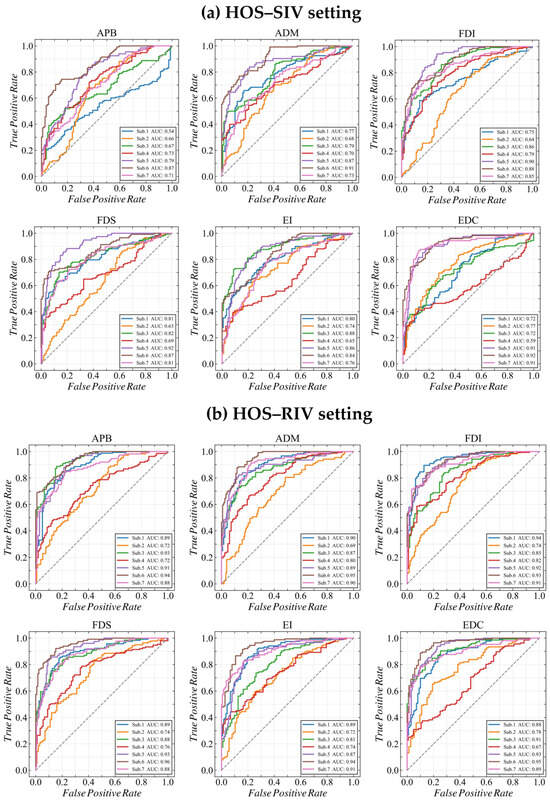
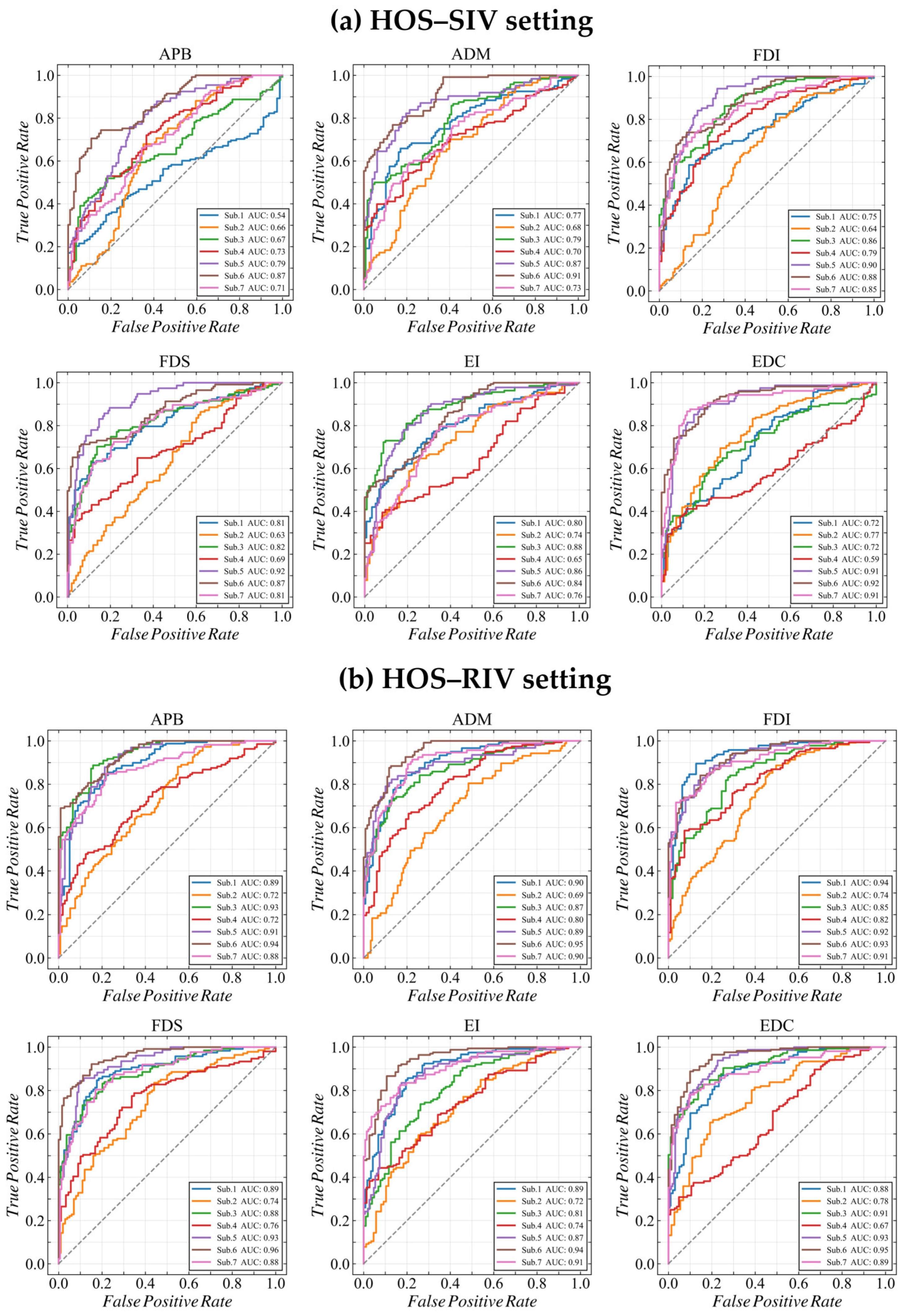
Figure 6 shows the ROC curves for each muscle and each outer test subject under the HOS-SIV and HOS-RIV settings. Under the HOS-SIV setting, participants 5, 6, and 7 showed consistently high ROC-AUC values across muscles, ranging from 0.71 to 0.92. In contrast, participants 1, 2, and 4 showed greater variability across muscles and generally lower ROC-AUC values. Notably, for the APB muscle in participant 1, the ROC-AUC value was relatively low compared with those of the other muscles. However, participant 1 had the highest MEP-positive rate for APB, as described in Section 3.1. In the HOS-RIV setting, the overall ROC-AUC values were higher than those in the HOS-SIV setting. Participants 2 and 4 exhibited lower predictive performance in some muscles, with ROC-AUC values decreasing to around 0.67, whereas the other participants showed consistently high ROC-AUC values across all muscles. As described in Section 3.1, participant 5, who had the lowest MEP-positive rate, nevertheless showed a high mean ROC-AUC of 0.91 (0.87–0.93). The largest difference in MEP-positive rate was observed for ADM between participant 4 (65.8%) and participant 5 (25.8%); however, the difference in ROC-AUC was small, at only 0.09 (participant 4: 0.80; participant 5: 0.89). These results suggest that the proportion of MEP-positive samples alone does not determine prediction performance.
Figure 6.
Receiver operating characteristic (ROC) curves for MEP prediction in each muscle (APB, ADM, FDI, FDS, EI, and EDC) under the (a) HOS-SIV and (b) HOS-RIV split settings. The x-axis indicates the false positive rate (FPR = FP/(FP + TN)), and the y-axis indicates the true positive rate (TPR = TP/(TP + FN)). Each colored curve represents one participant, and the corresponding area under the curve (AUC) is listed in the legend. The dashed diagonal line indicates chance-level performance. Curves closer to the upper-left corner indicate better discrimination between MEP presence and absence.
3.3. Effect of Model Architecture on Predictive Performance
The predictive performance is compared between conventional classifiers, simple CNN models, and ResNet-based models under the two inner-validation settings.
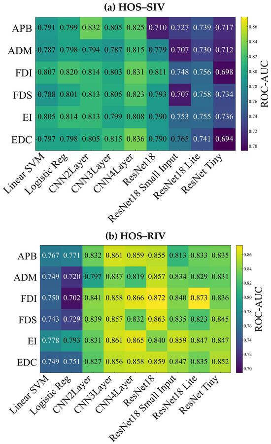
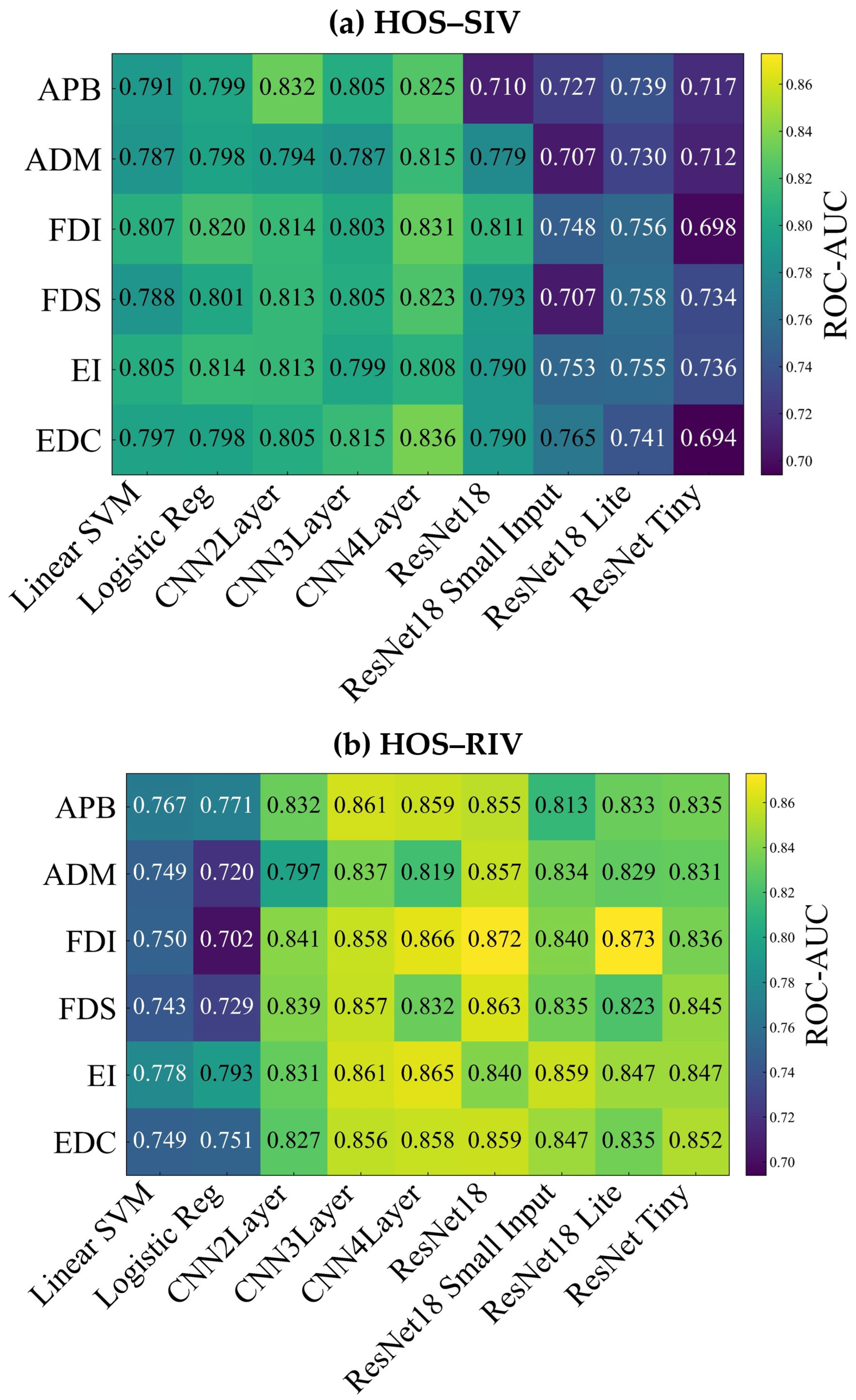
Figure 7a shows the results obtained using the HOS-SIV setting. The conventional classifiers achieved moderate predictive performance, with ROC-AUC values ranging from 0.787 to 0.807 for linear SVM and from 0.798 to 0.820 for logistic regression across muscles. Among the simple CNN models, CNN4Layer achieved the highest ROC-AUC across four of the six muscles, ranging from 0.808 to 0.836. The ResNet-based models generally showed lower ROC-AUC values than the conventional classifiers and CNN-based models (e.g., ResNet18, with ROC-AUC ranging from 0.710 to 0.811 across muscles).
Figure 7.
Heatmap comparison of ROC-AUC values across model architectures. (a) Results under the HOS-SIV inner-validation setting; (b) Results under the HOS-RIV inner-validation setting. Rows indicate target muscles, columns indicate model architectures, and the shared color scale represents ROC-AUC values across both heatmaps.
Figure 7b shows the results obtained using the HOS-RIV setting. The ROC-AUC values of linear SVM and logistic regression ranged from 0.743 to 0.778 and from 0.702 to 0.793, respectively, whereas most simple CNN and ResNet-based models achieved ROC-AUC values above 0.80 across muscles. Among them, ResNet18 showed consistently higher performance, with ROC-AUC values ranging from 0.840 to 0.872.
Statistical comparisons confirmed that model architecture did not significantly affect ROC-AUC under the primary HOS-SIV setting for any muscle. Under the secondary HOS-RIV setting, significant model effects were observed for APB, FDS, EI, and EDC, with selected CNN- or ResNet-based models outperforming linear SVM. These findings indicate that the advantage of convolutional architectures was not consistent under the stricter subject-wise validation scheme (Appendix D).
3.4. Agreement Between Measured and Predicted Spatial MEP Maps
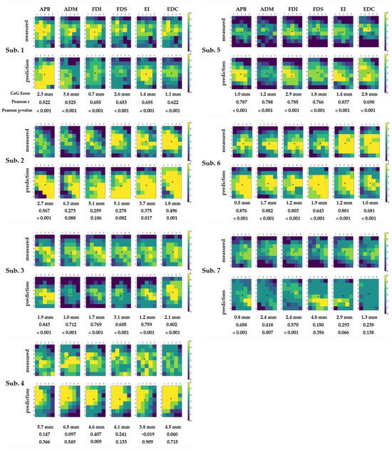
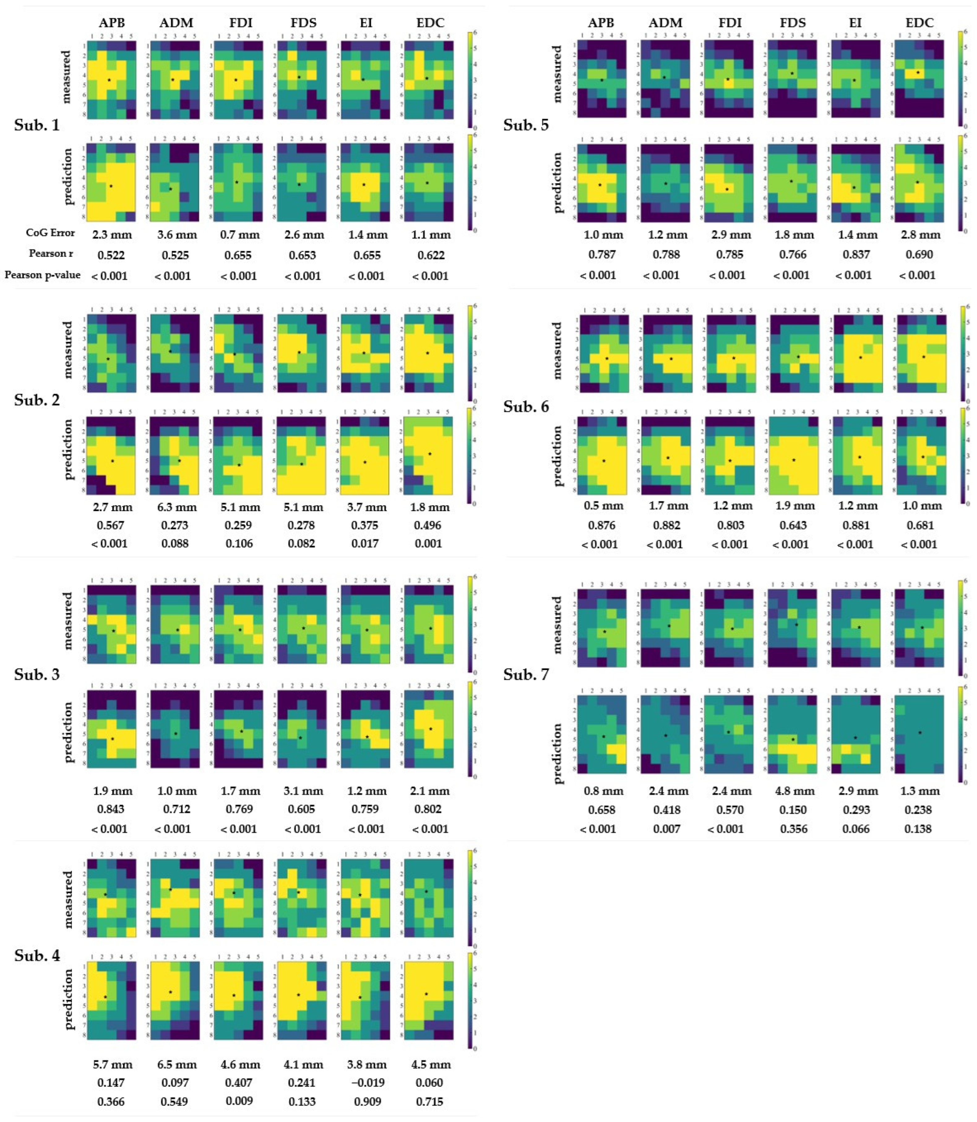
Figure 8 compares two-dimensional heatmaps of the measured and predicted MEP responses for each muscle under an HOS-RIV setting using ResNet18. The two-dimensional representation corresponds to the same 8 × 5 grid on which TMS was delivered (see Figure 1a). The number of MEP-positive responses at each grid ranged from 0 to 6, corresponding to the six stimulation conditions tested at that location: two stimulation intensities and three coil orientations. Then, the CoG error was the distance between the measured and predicted centroids. In addition, the Pearson correlation coefficient was computed between the measured and predicted heatmaps to assess similarity.
Figure 8.
Two-dimensional heatmaps of measured and predicted MEP response distributions for each muscle in each subject (Sub. 1 to Sub. 7) under the HOS-RIV setting. In each subject-specific panel, the upper row shows the measured distribution, and the lower row shows the predicted distribution. Each heatmap represents the spatial distribution of MEP responses on the stimulation grid. A black dot indicates the center of gravity of each distribution, and the center-of-gravity error was defined as the distance between the centers of gravity of the measured and predicted distributions. The Pearson correlation coefficient was also calculated for each heatmap pair to quantify the similarity between the measured and predicted spatial distributions.
The results show that the centroids of different muscles were closely clustered in most cases. In terms of the CoG error, the smallest was observed for APB in participant 6, at 0.5 mm. In contrast, participants 2 and 4, who showed relatively low ROC-AUC values, exhibited larger CoG errors than the other participants, ranging from 1.8 to 6.3 mm in participant 2 and from 3.8 to 6.5 mm in participant 4. Most of these errors were within the grid size of 5 mm.
In terms of the MEP heatmaps, the measured heatmaps revealed clear differences in distribution patterns, including differences in spread, concentration, and spatial bias. This indicates that the model did not simply generate a stereotyped output with nearly identical spatial patterns across all conditions. When comparing the measured and predicted maps, the Pearson correlation coefficients in participants with lower ROC-AUC values ranged from 0.259 to 0.567 and from −0.019 to 0.407 for participants 2 and 4, respectively. In contrast, relatively significant correlations were observed in most muscles of the other participants. The highest Pearson correlation coefficient was observed for ADM in participant 6 (r = 0.882).
4. Discussion
In this study, we investigated whether TMS-induced MEPs could be predicted from subject-specific intracranial E-field distributions using a compact two-dimensional representation of the motor cortex for the first time. As a proof of concept, this approach is practically relevant because predicting MEP responses under untested stimulation conditions may support more efficient TMS motor mapping.
4.1. Prediction from Subject-Specific E-Field Maps
The present study demonstrated the feasibility of predicting MEP elicitation in unseen test subjects using subject-specific E-field maps. These findings suggest that the spatial distribution of the cortical E-field contains meaningful information for predicting whether an MEP will be elicited. A recent deep-learning study reported that between-subject prediction performance was lower than within-subject prediction performance [15]. In contrast to the present approach, that study relied on coil position, coil orientation, and stimulation intensity, without incorporating subject-specific E-field simulations. Because the induced E-field more directly reflects the cortical stimulation produced after accounting for individual anatomy, subject-specific E-field maps may provide additional information for predicting MEP responses.
4.2. Influence of Inner-Validation
We compared two inner-loop validation strategies for hyperparameter optimization: HOS-SIV and HOS-RIV. HOS-SIV was treated as the primary analysis because both inner-loop validation and outer-loop testing were performed at the subject level, consistent with the intended application to unseen participants. Early stopping and hyperparameter selection were therefore based on performance on a participant not represented in the inner training set, providing a stricter assessment of subject-independent generalization.
HOS-RIV was evaluated as a secondary analysis. After one participant was held out for outer testing, samples from all six outer-training participants were randomly divided into inner-training and validation subsets. This strategy can stabilize model selection in a small dataset because validation samples are drawn from multiple participants and all outer-training participants remain represented during model fitting. In contrast, HOS-SIV relies on a single validation participant and may therefore yield higher variance in model selection for small datasets. The higher outer-test performance observed under HOS-RIV may thus reflect a trade-off between greater validation stability and weaker subject-level independence. However, HOS-RIV provides weaker subject-level independence than HOS-SIV. Although the outer-test participant remains completely excluded, the inner training and validation subsets may share participant-specific characteristics. In addition, spatial correlation among neighboring stimulation conditions is expected in TMS motor mapping, because adjacent coil positions are intentionally sampled to characterize spatial gradients in cortical E-fields and MEP responses. Thus, this correlation represents physiologically meaningful structure rather than duplicate sampling. Nevertheless, under HOS-RIV, spatially correlated samples from the same participant may be assigned to both inner-training and validation subsets, which may partly contribute to the higher performance observed under HOS-RIV. Accordingly, HOS-SIV provides the more direct assessment of unseen-subject generalization, whereas HOS-RIV should be interpreted as a complementary limited-data analysis. Future studies should evaluate spatially blocked or grouped validation strategies to further examine the influence of within-subject spatial autocorrelation.
4.3. Two-Dimensional Cortical Representation
A key feature of this study is the transformation of three-dimensional cortical E-field data into a compact two-dimensional cortical representation. This representation preserves the organization of the cortical sheet, including spatial relationships between gyral crowns and sulcal walls, making it well-suited for CNN-based learning of spatial patterns on the cortical surface (Appendix E). This results in a compact, physics-informed representation well suited for subject-specific analysis of TMS-induced E-fields. Compared with approaches that use three-dimensional E-field volumes as input [16], the proposed representation is computationally simpler and less sparse. Three-dimensional inputs typically include many voxels outside the cortical surface of interest, thereby increasing data dimensionality without necessarily providing additional information relevant to MEP generation. As a focused control analysis, Appendix F compared the proposed 2D input with a 3D input for APB prediction under the HOS-RIV setting. The 2D input achieved comparable or higher ROC-AUC values than the 3D input in most held-out subjects and substantially reduced training time. These results suggest that the 2D cortical representation retained sufficient information to predict MEPs while reducing the dimensionality and sparsity of the volumetric input. Therefore, the proposed 2D representation may provide an efficient input format for predicting TMS-induced MEPs from subject-specific E-field maps. However, broader evaluation across muscles and validation schemes is required. Also, graph neural networks may be evaluated for e-field data represented on surface meshes and compared with models using flattened field maps in future work.
4.4. Effect of Model Architecture
The comparison across model architectures provides further insight into the role of spatial feature learning in MEP prediction (Appendix D). Under the primary HOS-SIV setting, no significant differences between model architectures were observed for any muscle. Under the secondary HOS-RIV setting, significant post hoc differences were detected only for selected muscles, with CNN4Layer or ResNet18 outperforming the linear SVM. Thus, the present results do not demonstrate a consistent superiority of convolutional architectures over conventional classifiers. In selected HOS-RIV cases, CNN4Layer and ResNet18 benefited from the spatial organization of the two-dimensional E-field inputs (Appendix E). However, this spatial sensitivity does not necessarily translate into consistently superior performance relative to conventional classifiers, which may already capture substantial predictive information from global E-field characteristics and location-specific pixel values. Nevertheless, the significant advantages observed for CNN4Layer and ResNet18 over LinearSVC in selected muscles under HOS-RIV provide preliminary evidence that spatial feature learning may offer an additional benefit when model selection is more stable. This benefit may have been modest and difficult to detect consistently under HOS-SIV because of the limited number of participants available for subject-wise validation and evaluation with sufficient training data [37]. Future studies with larger, more diverse datasets and possibly higher-resolution cortical E-field representations are required to determine whether CNN- and ResNet-based models offer a clear advantage over conventional machine-learning classifiers for MEP prediction.
4.5. Heatmap Prediction
The heatmap evaluated whether predicted MEP responses preserve spatial response patterns within the stimulation grid. The predicted heatmaps partially reproduced the spatial structure of the measured MEP distributions, suggesting that the model retained spatial trends related to individualized E-field maps. Although the relatively small CoG errors do not necessarily indicate accurate spatial reconstruction, positive correlations between predicted and measured heatmaps were observed across most subject–muscle pairs, despite substantial variability in spatial distributions among subjects and muscles. It should also be noted that the heatmaps in this study were generated on the two-dimensional coil-position grid, rather than on the native three-dimensional cortical surface. This representation was used because it allows direct comparison between predicted responses and experimentally measured MEPs at each coil position. Therefore, future studies should validate the predicted heatmap to determine whether these predictions can guide the selection of stimulation targets in clinical motor mapping.
4.6. Limitations and Future Work
The present study presents some limitations. First, although the present study included more participants than the previous E-field-based MEP prediction study [16], the participants were limited to a small cohort of young, healthy volunteers, and the sex distribution was imbalanced, with a predominance of male participants. Therefore, this study should be regarded as a preliminary validation of the proposed framework. Larger and more diverse cohorts, including participants across a wider age range, balanced sex distributions, and clinical populations, will be required to confirm its robustness and generalizability. Second, TMS intensity was tested only at 100% and 120% of the resting motor threshold. Future studies should include a wider range of stimulation intensities to assess whether the proposed model generalizes across varying levels of cortical excitability. Third, MEP responses were treated as binary labels based on whether the peak-to-peak amplitude exceeded 50 μV. This binary classification approach is useful for evaluating the presence or absence of MEPs, but it does not capture the continuous variation in MEP amplitude required for brain mapping using regression-based models [38,39]. In the future, adopting multiscale neural modeling can bring an additional layer to predict activation with deep learning for more complex prediction on MEP waveform [32]. Fourth, the conventional machine-learning baselines were limited to logistic regression and linear SVM. Future studies should examine additional conventional classifiers, including nonlinear SVM kernels, and systematically optimize kernel-related hyperparameters within the same nested cross-validation framework.
5. Conclusions
This proof-of-concept study demonstrated a deep-learning-based prediction of TMS-induced MEPs from two-dimensional flattened cortical maps. Flattened cortical E-field representations preserve meaningful subject-specific biophysical information relevant to MEP elicitation while reducing the dimensionality of the original three-dimensional E-field data. Overall, the results support the feasibility of using individualized cortical E-field maps for MEP prediction and provide a basis for future studies aimed at reducing empirical sampling in TMS motor mapping. Further validation in larger and more diverse cohorts will be required.
Author Contributions
Conceptualization, J.G.-T.; methodology, all; software, H.T.; validation, H.T. and J.G.-T.; formal analysis, H.T. and J.G.-T.; investigation, H.T. and J.G.-T.; resources, M.F. and J.G.-T.; data curation, H.T. and J.G.-T.; writing—original draft preparation, H.T. and J.G.-T.; writing—review and editing, all; visualization, H.T. and J.G.-T.; supervision, W.Y. and J.G.-T.; project administration, J.G.-T.; funding acquisition, M.F. and J.G.-T. All authors have read and agreed to the published version of the manuscript.
Funding
This study was supported by the JSPS Grant-in-Aid for Scientific Research (JSPS KAKENHI Grant No. 25K15887), the JSPS Program for Forming Japan’s Peak Research (J-PEAKS, Grant No. JPJS00420230002), and the Joint Research Program (25NIPS632) of the National Institute for Physiological Sciences and MEXT/CURE JPMXP1323015488 (Spin-L program No. spin25XN050).
Institutional Review Board Statement
The study was conducted in accordance with the Declaration of Helsinki and approved by the Ethics Committees of Chiba University (approval code: R6-33; approval date: 31 March 2025) and the National Institute of Natural Sciences (approval code: EC01-098, 23 April 2025).
Informed Consent Statement
Written informed consent has been obtained from the patient(s) to publish this paper.
Data Availability Statement
Source code and processed flattened cortical E-field maps used for model training and evaluation will be made available at https://github.com/Haruto2000001/mep-prediction-from-efield-maps (accessed on 23 July 2026).
Conflicts of Interest
The authors declare no conflicts of interest.
Appendix A. Cortical Gyrification Difference
Figure A1 shows the precentral cortex for each participant. This illustrates inter-subject variability in the morphology and spatial extent of the precentral cortex, even within this relatively homogeneous cohort. Because cortical geometry affects the spatial distribution of TMS-induced E-fields, this anatomical variability helps explain why unseen-subject prediction remains non-trivial.
Figure A1.
Visualization of the precentral cortex in the seven participants. The red region indicates the gray matter surface corresponding to the precentral cortex. Participant characteristics were as follows: Sub. 1, 23 years, male, RMT 65%; Sub. 2, 19 years, male, RMT 53%; Sub. 3, 22 years, male, RMT 50%; Sub. 4, 21 years, male, RMT 58%; Sub. 5, 23 years, male, RMT 62%; Sub. 6, 23 years, female, RMT 62%; and Sub. 7, 23 years, male, RMT 56%.
Appendix B. Training and Validation Loss Curves
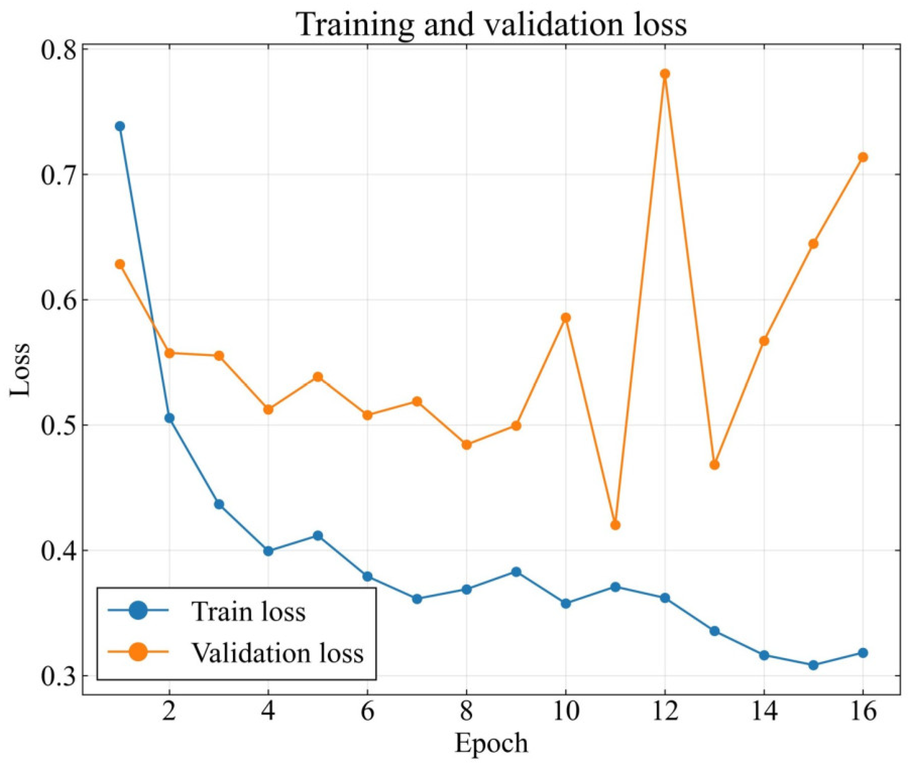
Figure A2 shows one representative training and validation loss curve for the ResNet-based model. Similar loss-curve behavior was observed across the other training runs, confirming that Figure A2 is representative. The training loss decreased steadily across epochs, indicating that the model parameters were optimized during training. In contrast, the validation loss fluctuated and began to increase after reaching its minimum. This illustrates the rationale for applying early stopping based on validation loss to reduce overfitting, and the model checkpoint with the lowest validation loss was used for test-set evaluation. This procedure was performed within the inner loop of the nested cross-validation, without using the held-out outer test participant.
Figure A2.
Representative training and validation loss curves for the ResNet-based model.
Appendix C. Additional Evaluation Metrics
Table A1 and Table A2 present additional threshold-dependent evaluation metrics for the outer test data under the HOS-SIV and HOS-RIV settings, respectively. Specifically, accuracy, recall, precision, and F1-score are reported as mean ± standard deviation across the outer test folds, with 95% confidence intervals shown in brackets. Predicted probabilities were binarized using a fixed threshold of 0.3 for threshold-dependent metrics such as the F1-score. This threshold was determined before test-set evaluation by averaging the F1-score-optimized thresholds from the validation folds and rounding the result to the nearest 0.1. The held-out test data were not used for threshold selection.
Compared with the ROC-AUC values reported in the main text, these threshold-dependent metrics tended to be lower and exhibit greater variability across outer test folds. This difference may be partly explained by the use of a fixed probability threshold for binarizing predicted probabilities. The relatively wide confidence intervals, particularly for recall and F1-score, suggest that these threshold-dependent metrics were sensitive to inter-participant variability and to the selected decision threshold. For this reason, ROC-AUC was used as the primary performance metric in the main text, whereas the threshold-dependent metrics are provided here.
Table A1.
Additional Model performance under the HOS-SIV setting, reported mean ± SD [95% CI].
Table A2.
Additional Model performance under the HOS-RIV setting, reported mean ± SD [95% CI].
Appendix D. Statistical Analysis Among Model Architectures
To examine whether the apparent differences in ROC-AUC among model architectures were statistically significant, paired statistical analyses were performed across the same outer test folds. For each muscle and validation setting, a Friedman test was first applied across model architectures, and Kendall’s W was calculated as an effect-size measure. When the Friedman test was significant, post hoc paired comparisons were performed, and p-values were adjusted using the Holm correction. The paired mean difference in ROC-AUC (Δ), the 95% confidence interval, and the Holm-adjusted p-value are reported.
Table A3 summarizes the statistical comparisons among model architectures based on ROC-AUC. No statistically significant differences among model architectures were observed under the primary HOS-SIV setting for any muscle. The Friedman p values ranged from 0.180 to 0.651, and Kendall’s W ranged from 0.061 to 0.245, indicating small to moderate effect sizes. In contrast, under the secondary HOS-RIV setting, significant model effects were observed for APB, FDS, EI, and EDC. Post hoc comparisons showed that CNN4Layer significantly outperformed Linear SVM on APB, FDS, and EI. ResNet18 also significantly outperformed Linear SVM for FDS and EDC.
Table A3.
Summary of statistical comparisons among model architectures based on ROC-AUC.
Appendix E. Spatial Information in the Two-Dimensional E-Field Maps
To investigate the importance of spatial information in the two-dimensional E-field maps for CNN and ResNet under HOS-RIV, a spatial-shuffling control analysis was performed for the model–muscle combinations that showed significant post hoc differences in Table A3. As illustrated in Figure A3, a single fixed random permutation was applied identically to all input maps. This procedure preserved the distribution of E-field values within each sample while disrupting the original cortical neighborhood structure and local spatial continuity of the 2D maps. Using the shuffled inputs, the same training and evaluation procedure used in this study was repeated, and the resulting ROC-AUC values were compared with those obtained using the original inputs.
Table A4 summarizes the results of spatial-shuffling control analysis. Original-input and shuffled-input models were compared using paired outer-fold ROC-AUC values, and FDR correction was applied across the tested comparisons. In all tested conditions, the original-input models significantly outperformed the shuffled-input models after FDR correction. Significant differences were observed for CNN4Layer in APB, FDS, and EI, and for ResNet18 in FDS and EDC.
These results suggest that for the model–muscle combinations that showed significant post hoc differences under HOS-RIV, the performance advantages of CNN4Layer and ResNet18 depended at least in part on the spatial organization of the two-dimensional cortical E-field maps. However, because this control analysis was applied only to the significant HOS-RIV comparisons identified in Table A4, the results should be interpreted as supporting the contribution of spatial organization in those specific cases, rather than as evidence for a general advantage of deep-learning architecture across all muscles or validation settings.
Figure A3.
A fixed random permutation was applied to all samples. This control preserved the E-field (EF) values but disrupted the original spatial arrangement of the cortical map.
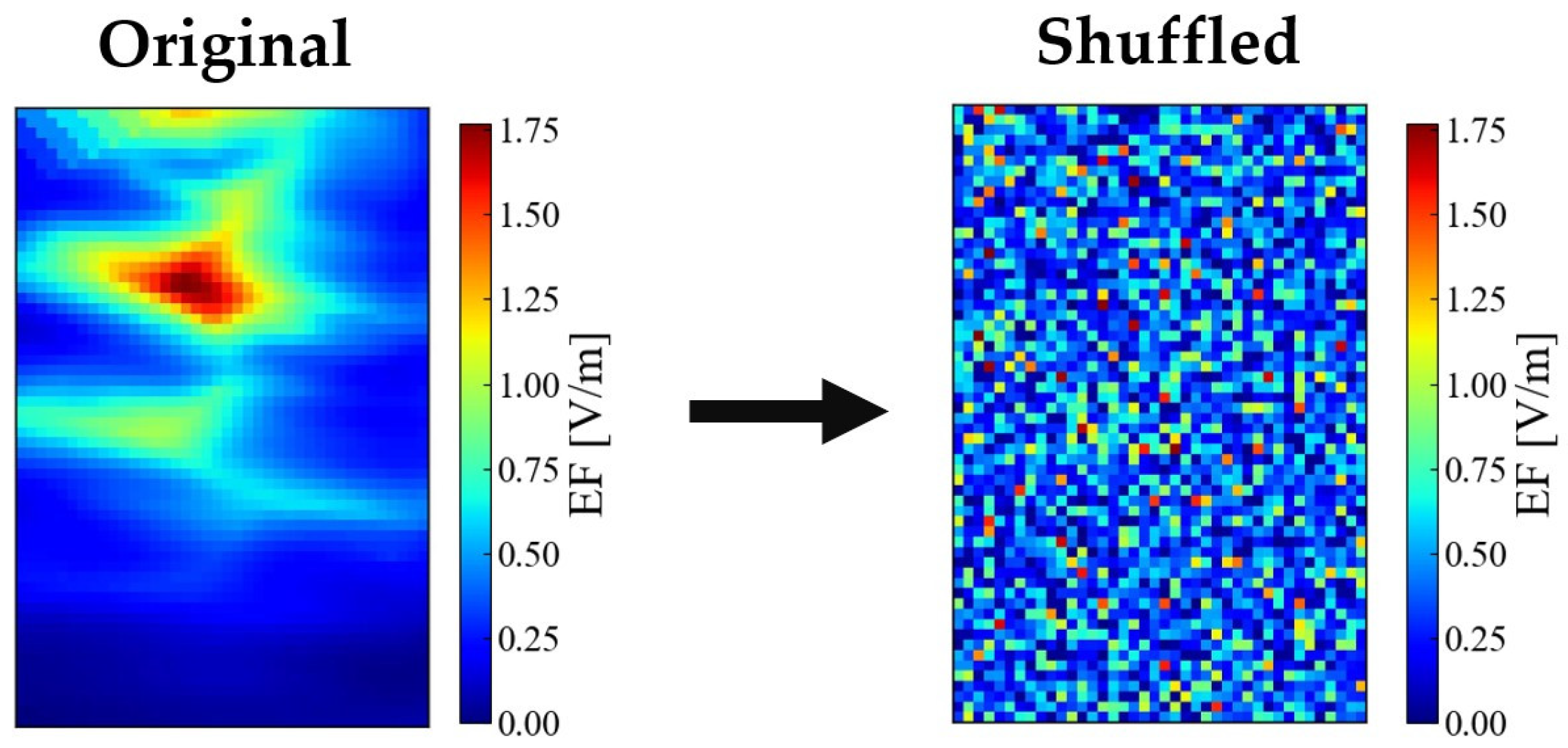
Table A4.
ROC-AUC-based spatial-shuffling control for significant HOS-RIV cases.
Appendix F. Comparison of 2D and 3D E-Field Inputs
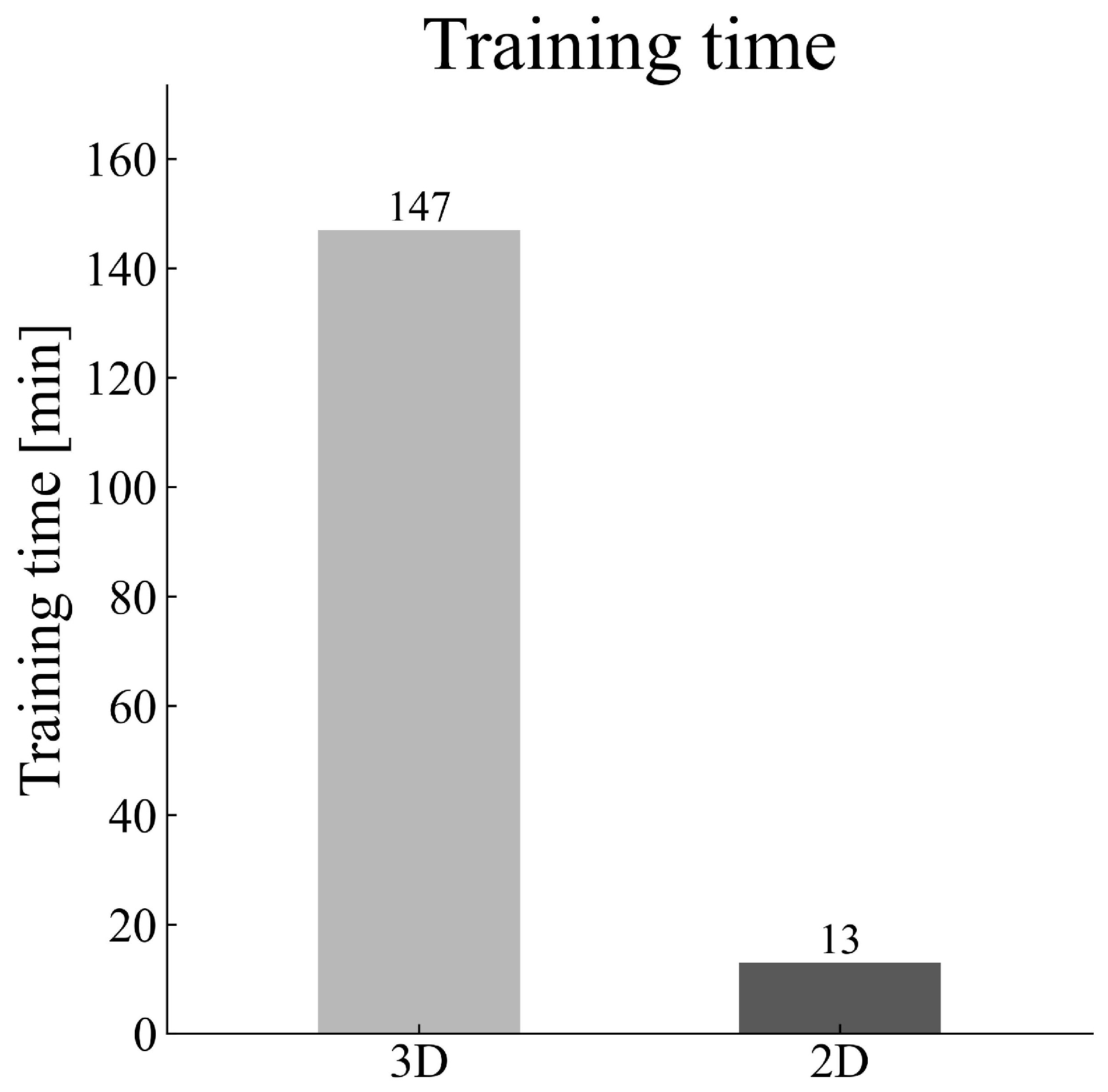
We compared the proposed 2D input with a 3D input for APB prediction under the HOS-RIV inner-validation setting. For the 3D input, the E-field distribution was extracted from the motor cortical region and resampled into a 64 × 64 × 64 volume. Three-dimensional versions of ResNet18 and CNN4Layer were then trained and evaluated using the same procedure as the 2D models. As shown in Figure A4, the 2D input achieved comparable or higher ROC-AUC values than the 3D input in most cases. In particular, 2D ResNet18 outperformed 3D ResNet18 across all seven test subjects (p = 0.0016, FDR-adjusted p = 0.0032), while 2D CNN4Layer showed comparable or higher performance in several subjects compared with 3D CNN4Layer (p = 0.1440, FDR-adjusted p = 0.1440). Using ResNet18 with the HOS-RIV split, the 2D representation substantially reduced training time from 147 min for the 3D input to 13 min for the 2D input (Figure A5). All models were implemented in PyTorch 2.9.1 and trained on a workstation equipped with an Intel Xeon w3-2435 CPU (8 cores, 3.1 GHz), an NVIDIA RTX 4000 SFF Ada GPU (20 GB), and 64 GB RAM.
Figure A4.
Comparison of ROC-AUC values between 3D and 2D E-field inputs for APB prediction in the HOS-RIV inner-validation setting. (a) Results obtained using ResNet18; (b) Results obtained using CNN4Layer. For the 3D input, the E-field distribution was extracted from the motor cortical region and represented as a 64 × 64 × 64 volume. For the 2D input, the same cortical E-field information was represented as a flattened cortical map. Bars indicate the ROC-AUC values for each held-out test subject. Light blue and dark blue bars indicate the 3D and 2D inputs, respectively.
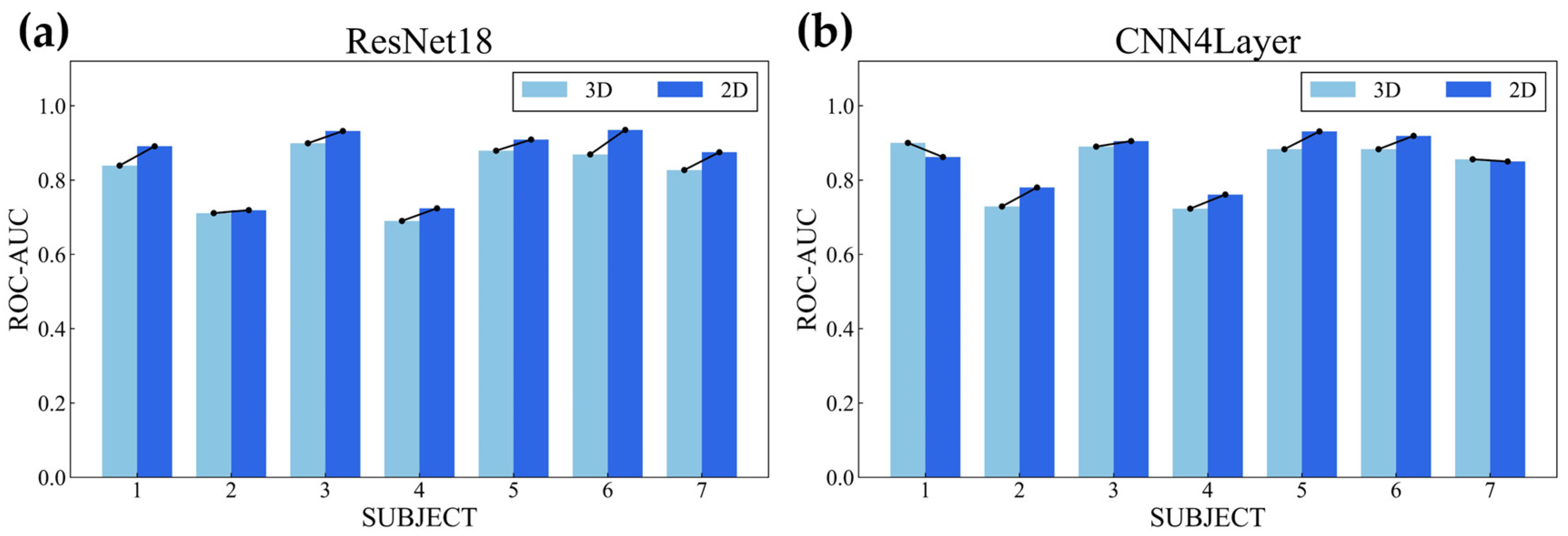
Figure A5.
Comparison of training time between 3D and 2D E-field inputs. Training time obtained using ResNet18 under the HOS-RIV setting; the 3D and 2D inputs required 147 min and 13 min, respectively.
References
- Barker, A.T.; Jalinous, R.; Freeston, I.L. Non-invasive magnetic stimulation of human motor cortex. Lancet 1985, 325, 1106–1107. [Google Scholar] [CrossRef] [Scilit]
- Bestmann, S.; Krakauer, J.W. The uses and interpretations of the motor-evoked potential for understanding behaviour. Exp. Brain Res. 2015, 233, 679–689. [Google Scholar] [CrossRef] [Scilit] [PubMed]
- Bastani, A.; Jaberzadeh, S. A Higher Number of TMS-Elicited MEP from a Combined Hotspot Improves Intra- and Inter-Session Reliability of the Upper Limb Muscles in Healthy Individuals. PLoS ONE 2012, 7, e47582. [Google Scholar] [CrossRef] [Scilit] [PubMed]
- Takahashi, S.; Vajkoczy, P.; Picht, T. Navigated transcranial magnetic stimulation for mapping the motor cortex in patients with rolandic brain tumors. Neurosurg. Focus 2013, 34, E3. [Google Scholar] [CrossRef] [Scilit] [PubMed]
- Raffa, G.; Scibilia, A.; Conti, A.; Ricciardo, G.; Rizzo, V.; Morelli, A.; Angileri, F.F.; Cardali, S.M.; Germanò, A. The role of navigated transcranial magnetic stimulation for surgery of motor-eloquent brain tumors: A systematic review and meta-analysis. Clin. Neurol. Neurosurg. 2019, 180, 7–17. [Google Scholar] [CrossRef] [Scilit] [PubMed]
- Kozel, F.A.; Nahas, Z.; deBrux, C.; Molloy, M.; Lorberbaum, J.P.; Bohning, D.; Risch, S.C.; George, M.S. How Coil–Cortex Distance Relates to Age, Motor Threshold, and Antidepressant Response to Repetitive Transcranial Magnetic Stimulation. J. Neuropsychiatry Clin. Neurosci. 2000, 12, 376–384. [Google Scholar] [CrossRef] [PubMed]
- Gomez-Tames, J.; Hamasaka, A.; Laakso, I.; Hirata, A.; Ugawa, Y. Atlas of optimal coil orientation and position for TMS: A computational study. Brain Stimul. 2018, 11, 839–848. [Google Scholar] [CrossRef] [Scilit] [PubMed]
- Janssen, A.M.; Oostendorp, T.F.; Stegeman, D.F. The effect of local anatomy on the electric field induced by TMS: Evaluation at 14 different target sites. Med. Biol. Eng. Comput. 2014, 52, 873–883. [Google Scholar] [CrossRef] [Scilit] [PubMed]
- Saturnino, G.B.; Madsen, K.H.; Thielscher, A. Electric field simulations for transcranial brain stimulation using FEM: An efficient implementation and error analysis. J. Neural Eng. 2019, 16, 066032. [Google Scholar] [CrossRef] [Scilit] [PubMed]
- Gomez-Tames, J.; Laakso, I.; Hirata, A. Review on biophysical modelling and simulation studies for transcranial magnetic stimulation. Phys. Med. Biol. 2020, 65, 24TR03. [Google Scholar] [CrossRef] [Scilit] [PubMed]
- Koponen, L.M.; Martinez, M.; Wood, E.; Murphy, D.L.K.; Goetz, S.M.; Appelbaum, L.G.; Peterchev, A.V. Transcranial magnetic stimulation input–output curve slope differences suggest variation in recruitment across muscle representations in primary motor cortex. Front. Hum. Neurosci. 2024, 18, 1310320. [Google Scholar] [CrossRef] [Scilit] [PubMed]
- Bungert, A.; Antunes, A.; Espenhahn, S.; Thielscher, A. Where does TMS Stimulate the Motor Cortex? Combining Electrophysiological Measurements and Realistic Field Estimates to Reveal the Affected Cortex Position. Cereb. Cortex. 2016, 27, 5083–5094. [Google Scholar] [CrossRef] [Scilit]
- Weise, K.; Numssen, O.; Thielscher, A.; Hartwigsen, G.; Knösche, T.R. A novel approach to localize cortical TMS effects. NeuroImage 2020, 209, 116486. [Google Scholar] [CrossRef] [Scilit] [PubMed]
- Tervo, A.E.; Metsomaa, J.; Nieminen, J.O.; Sarvas, J.; Ilmoniemi, R.J. Automated search of stimulation targets with closed-loop transcranial magnetic stimulation. NeuroImage 2020, 220, 117082. [Google Scholar] [CrossRef] [Scilit] [PubMed]
- Jin, F.; Bruijn, S.M.; Daffertshofer, A. Machine learning approaches to predict whether MEPs can be elicited via TMS. J. Neurosci. Methods 2024, 410, 110242. [Google Scholar] [CrossRef] [Scilit] [PubMed]
- Akbar, M.N.; Yarossi, M.; Martinez-Gost, M.; Sommer, M.A.; Dannhauer, M.; Rampersad, S.; Brooks, D.; Tunik, E.; Erdoğmuş, D. Mapping Motor Cortex Stimulation to Muscle Responses: A Deep Neural Network Modeling Approach. In Proceedings of the 13th ACM International Conference on PErvasive Technologies Related to Assistive Environments, Corfu, Greece, 30 June–3 July 2020; pp. 1–6. [Google Scholar]
- Akbar, M.N.; Yarossi, M.; Rampersad, S.; Lockwood, K.; Masoomi, A.; Tunik, E.; Brooks, D.; Erdoğmuş, D. M2M-InvNet: Human Motor Cortex Mapping From Multi-Muscle Response Using TMS and Generative 3D Convolutional Network. IEEE Trans. Neural Syst. Rehabil. Eng. 2024, 32, 1455–1465. [Google Scholar] [CrossRef] [Scilit] [PubMed]
- Fischl, B.; Sereno, M.I.; Dale, A.M. Cortical Surface-Based Analysis: II: Inflation, Flattening, and a Surface-Based Coordinate System. NeuroImage 1999, 9, 195–207. [Google Scholar] [CrossRef] [Scilit] [PubMed]
- Richter, L.; Neumann, G.; Oung, S.; Schweikard, A.; Trillenberg, P. Optimal Coil Orientation for Transcranial Magnetic Stimulation. PLoS ONE 2013, 8, e60358. [Google Scholar] [CrossRef] [Scilit] [PubMed]
- Rossini, P.M.; Barker, A.T.; Berardelli, A.; Caramia, M.D.; Caruso, G.; Cracco, R.Q.; Dimitrijević, M.R.; Hallett, M.; Katayama, Y.; Lücking, C.H. Non-invasive electrical and magnetic stimulation of the brain, spinal cord and roots: Basic principles and procedures for routine clinical application. Report of an IFCN committee. Electroencephalogr. Clin. Neurophysiol. 1994, 91, 79–92. [Google Scholar] [CrossRef] [Scilit] [PubMed]
- Karabanov, A.N.; Raffin, E.; Siebner, H.R. The Resting Motor Threshold—Restless or Resting? A Repeated Threshold Hunting Technique to Track Dynamic Changes in Resting Motor Threshold. Brain Stimul. 2015, 8, 1191–1194. [Google Scholar] [CrossRef] [Scilit] [PubMed]
- Osnabruegge, M.; Kanig, C.; Schwitzgebel, F.; Litschel, K.; Seiberl, W.; Mack, W.; Schecklmann, M.; Schoisswohl, S. On the reliability of motor evoked potentials in hand muscles of healthy adults: A systematic review. Front. Hum. Neurosci. 2023, 17, 1237712. [Google Scholar] [CrossRef] [Scilit] [PubMed]
- Thielscher, A.; Antunes, A.; Saturnino, G.B. Field modeling for transcranial magnetic stimulation: A useful tool to understand the physiological effects of TMS? In Proceedings of the 2015 37th Annual International Conference of the IEEE Engineering in Medicine and Biology Society (EMBC), Milan, Italy, 25–29 August 2015; pp. 222–225. [Google Scholar]
- Wagner, T.A.; Zahn, M.; Grodzinsky, A.J.; Pascual-Leone, A. Three-Dimensional Head Model Simulation of Transcranial Magnetic Stimulation. IEEE Trans. Biomed. Eng. 2004, 51, 1586–1598. [Google Scholar] [CrossRef] [Scilit] [PubMed]
- Dannhauer, M.; Lanfer, B.; Wolters, C.H.; Knösche, T.R. Modeling of the human skull in EEG source analysis. Hum. Brain Mapp. 2011, 32, 1383–1399. [Google Scholar] [CrossRef] [Scilit] [PubMed]
- Goncalves, S.I.; de Munck, J.C.; Verbunt, J.P.A.; Bijma, F.; Heethaar, R.M.; Lopes da Silva, F. In vivo measurement of the brain and skull resistivities using an eit-based method and realistic models for the head. IEEE Trans. Biomed. Eng. 2003, 50, 754–767. [Google Scholar] [CrossRef] [Scilit] [PubMed]
- Köhler, M.; Götz, S. TMS coil design instrument (Kl/Codein Box): A toolbox for creating user-defined coils from conductor path data. Brain Stimul. 2023, 16, 698–700. [Google Scholar] [CrossRef] [Scilit] [PubMed]
- Di Lazzaro, V.; Ziemann, U. The contribution of transcranial magnetic stimulation in the functional evaluation of microcircuits in human motor cortex. Front. Neural Circuits 2013, 7, 18. [Google Scholar] [CrossRef] [Scilit] [PubMed]
- Macdonell, R.A.L.; Jackson, G.D.; Curatolo, J.M.; Abbott, D.F.; Berkovic, S.F.; Carey, L.M.; Syngeniotin, A.; Fabinyi, G.; Scheffer, I. Motor cortex localization using functional MRI and transcranial magnetic stimulation. Neurology 1999, 53, 1462–1467. [Google Scholar] [CrossRef] [Scilit] [PubMed]
- Desikan, R.S.; Ségonne, F.; Fischl, B.; Quinn, B.T.; Dickerson, B.C.; Blacker, D.; Buckner, R.L.; Dale, A.M.; Maguire, R.P.; Hyman, B.T.; et al. An automated labeling system for subdividing the human cerebral cortex on MRI scans into gyral based regions of interest. NeuroImage 2006, 31, 968–980. [Google Scholar] [CrossRef] [Scilit] [PubMed]
- Raemaekers, M.; Bruurmijn, M.; Ramsey, N. The brain in a box: A toolbox for creating Cartesian geometric representations with isometric dimensions (Cgrids). J. Neurosci. Methods 2020, 339, 108738. [Google Scholar] [CrossRef] [Scilit] [PubMed]
- Gomez–Tames, J.; Laakso, I.; Murakami, T.; Ugawa, Y.; Hirata, A. TMS activation site estimation using multiscale realistic head models. J. Neural Eng. 2020, 17, 036004. [Google Scholar] [CrossRef] [Scilit] [PubMed]
- Ioffe, S.; Szegedy, C. Batch Normalization: Accelerating Deep Network Training by Reducing Internal Covariate Shift. In Proceedings of the 32nd International Conference on Machine Learning, Lille, France, 7–9 July 2015; Volume 37, pp. 448–456. [Google Scholar]
- He, K.; Zhang, X.; Ren, S.; Sun, J. Deep Residual Learning for Image Recognition. In Proceedings of the 2016 IEEE Conference on Computer Vision and Pattern Recognition (CVPR), Las Vegas, NV, USA, 27–30 June 2016; pp. 770–778. [Google Scholar]
- Loshchilov, I.; Hutter, F. Decoupled Weight Decay Regularization. In Proceedings of the International Conference on Learning Representations 2019, New Orleans, LA, USA, 6–9 May 2019. [Google Scholar]
- Wainer, J.; Cawley, G. Nested cross-validation when selecting classifiers is overzealous for most practical applications. Expert Syst. Appl. 2021, 182, 115222. [Google Scholar] [CrossRef] [Scilit]
- Alzubaidi, L.; Zhang, J.; Humaidi, A.J.; Al-Dujaili, A.; Duan, Y.; Al-Shamma, O.; Santamaría, J.; Fadhel, M.A.; Al-Amidie, M.; Farhan, L. Review of deep learning: Concepts, CNN architectures, challenges, applications, future directions. J. Big Data 2021, 8, 53. [Google Scholar] [CrossRef] [Scilit] [PubMed]
- Diekhoff, S.; Uludağ, K.; Sparing, R.; Tittgemeyer, M.; Cavuşoğlu, M.; von Cramon, D.Y.; Grefkes, C. Functional localization in the human brain: Gradient-echo, spin-echo, and arterial spin-labeling fMRI compared with neuronavigated TMS. Hum. Brain Mapp. 2011, 32, 341–357. [Google Scholar] [CrossRef] [Scilit] [PubMed]
- Numssen, O.; Zier, A.L.; Thielscher, A.; Hartwigsen, G.; Knösche, T.R.; Weise, K. Efficient high-resolution TMS mapping of the human motor cortex by nonlinear regression. NeuroImage 2021, 245, 118654. [Google Scholar] [CrossRef] [Scilit] [PubMed]

Disclaimer/Publisher’s Note: The statements, opinions and data contained in all publications are solely those of the individual author(s) and contributor(s) and not of MDPI and/or the editor(s). MDPI and/or the editor(s) disclaim responsibility for any injury to people or property resulting from any ideas, methods, instructions or products referred to in the content. |
© 2026 by the authors. Licensee MDPI, Basel, Switzerland. This article is an open access article distributed under the terms and conditions of the Creative Commons Attribution (CC BY) license.