The MiniMarket80 Dataset for Evaluation of Unique Item Segmentation in Point Clouds

Abstract

The effectiveness of deep learning methods in image segmentation has led to interest in their deployment for 3D point cloud segmentation, particularly in the context of pre-grasp identification of a unique object amongst distractors. However, existing 3D object datasets are not ideal for training and evaluation of these methods. Datasets developed for grasp planning are often CAD models that are too clean for sim-to-real transfer. Real-world datasets can lack texture information or have been collected using sets of objects and/or specialized sensor setups that are hard to reproduce. In this work, we introduce the MiniMarket80 dataset to address this gap.The dataset consists of 1200 colored point cloud partial views, each of 80 standard grocery objects, collected with widely used Realsense RGB-D cameras (D415 and D435) under variable lighting conditions. We also provide a complete pipeline to generate a per-object segmentation dataset from these partial views suitable for use in training. We use this dataset to evaluate 11 state-of-the-art point cloud segmentation methods. Only four of these are able to (partially) segment the target object in a real-world test, still producing significant false positives and false negatives.

1. Introduction

Robots are often required to grasp a specific object from a cluttered set of similar objects. A standard robot grasping system thus includes three critical elements: object identification/segmentation; grasp planning; and gripper design. Although the relationship between grasp planning and gripper geometry is well understood, the interaction of object segmentation methodology and the type of end-effector employed is often overlooked. Typically, segmentation methodologies used in the context of grasping automation are trained on conventional 2D image datasets [1,2,3], promoting the use of simple grippers (e.g., two-fingered or suction types) [4,5,6,7,8] in a top-down, 2D planning framework. In this paradigm, depth information is often reduced to determining the vertical approach of the gripper [6,9], resulting in a 2.5D grasping process. While 2D grasp planning would be sufficient for top-down bin picking or side shelving applications—currently dominating grasping research due to industrial interest in warehouse automation—other critical and emerging applications require 3D grasping. This includes the use of simple grippers to grasp from any direction around the object and the use of more complex end-effectors such as multifinger hands. Examples include industrial kitting [10], assisted living [11], humanoid service robots [12] or even—in the warehouse scenario—untidy bins.

It is thus essential to advance 3D object segmentation in pointclouds (discrete sets of data points representing the location and properties of points on surfaces in 3D space). Current solutions to this problem are dominated by deep learning approaches that in turn require vast realistic 3D object datasets. In the context of robotic grasping, several 3D object datasets have been made available. One of the first was the Princeton Shape Benchmark [13], a collection of CAD models retrieved online, followed by the Colombia Grasp Database, which is based on the CAD models of the Princeton Shape Benchmark in four different scales, with the addition of grasp candidates generated by the GraspIt! [14] simulator. The expansion of CAD model-based datasets continued with 3DNet [15], consisting of 3655 CAD models intended for object class recognition and pose estimation learning. Further datasets include ModelNet [16] (130 K models), ShapeNet [17] (3 M models) and Objaverse-XL [18] (10.2 M models), compiled by web crawling a variety of online sources and aimed at enabling a natural language processing-like breakthrough in 3D vision. A summary of these datasets is presented in Table 1, including an assessment of reproducibility, defined as how easy it is to obtain these dataset objects for comparative real-world evaluation. For simplicity, this can be categorized as “low” for objects that are very difficult to obtain in the real world, “medium” for those with limited global availability, or “high” for items easily found worldwide.

Table 1. Summary of 3D object grasping datasets in chronological order, hyperlinked to the respective hosting repositories. Attention is given primarily for object model datasets that have been used in data-driven grasping.

Dataset		Unique Objects	Object Samples	Grasp Candidates	CAD/Real	Year	Data Source	Reproduc- ability
1	Princeton ShapeBenchmark [13]	1814	1814 mesh models	−	CAD	2004	online, from 293 different web domains	low
2	Columbia GraspDatabase [19]	7256	7256 mesh models	238,737 for 2 hand models	CAD	2009	Princeton Shape Benchmark [13]	low
3	Cornell GraspingDataset [20]	224	885 images+ 885 depth maps	5310∼ 7080	Real	2011	author collected	low
4	RGB-D ObjectDataset [21]	300	250 K RGB-D	−	Real	2011	author collected	low
5	KIT ObjectDatabase [22]	152	608 textured meshes + 110 K images	for 3 types of grippers	Real	2012	author collected	medium
6	3DNet [15]	3433	3433 mesh models + 3200 RGB-D test scenes	−	CAD	2012	online 3D model repositories	low
7	BigBIRD [23]	100	60 K RGB-D + 60 K images	−	Real	2014	author collected	medium
8	YCB Object andModel Set [24]	77	46 K RGB-D + 46 K images + 77 textured meshes	−	Real	2015	author collected	medium
9	ModelNet [16]	128 K	127,915 mesh models	−	CAD	2015	261 CAD model websites	low
10	ShapeNet [17]	3 M	3 M mesh models	−	CAD	2015	online 3D model repositories	low
11	Dex-Net 1.0 [25]	13,252	13,252 mesh models	2.5 M	355 Real + 12,897 CAD	2016	KIT [22], BigBIRD [23], YCB [24], SHREC [26], 3DNet [15], ModelNet [16]	low
12	Jacquard [27]	11,619	54,485 RGB-D scenes	1,181,330	CAD	2018	ShapeNet [17]	low
13	EGAD [28]	2331	2331 meshes	∼1 M	imaginary CAD	2020	author generated	high
14	GraspNet-1Billion [29]	88	97,280 RGB-D images of 190 cluttered scenes + 88 textured meshes	∼1 B	Real	2020	32 of YCB [24] + 13 of Dex-Net 1.0 [25] + 43 author collected	medium
15	ACRONYM [30]	8872	8872 mesh models	17.744 M	CAD	2021	ShapeNet [17]	low
16	OCRTOC [31]	154	6 K labelled RGB-D images for 76 RGB-D scenes + 154 textured meshes	−	Real	2022	54 of YCB [24] + 101 author collected	medium
17	MetaGraspNet [32]	82	217 K RGB-D synthetic images + 2.3 K RGB-D real bin scenes	for vacuum and parallel- jaw grippers	73 Real + 9 CAD	2022	33 of YCB [24] + 4 of OCRTOC [31] + 45 author collected	medium
18	REGRAD [33]	50 K	900 K RGB-D synthetic images + 111.8 K scenes	100 M	CAD	2022	ShapeNet [17]	low
19	Objaverse-XL [18]	10.2 M	10.2 M mesh models	−	CAD	2023	online 3D model repositories	low
20	MetaGraspNetV2 [34]	82	296 K RGB-D synthetic images + 3.2 K RGB-D real bin scenes	for vacuum and parallel- jaw grippers	73 Real + 9 CAD	2024	33 of YCB [24] + 4 of OCRTOC [31] + 45 author collected	medium
21	MiniMarket80 (ours)	80	96 K RGB-D images	−	Real	2025	author collected	high

Other CAD-based datasets focused on expanding the grasp candidates generated in simulation as in Jacquard [27] and ACRONYM [30]. The REGRAD [33] is based on ModelNet and particularly addresses the relationship between objects in clutter and the order in which grasping should be executed. A notable deviation from the CAD-based datasets is EGAD [28], a collection of imaginary objects motivated by the fact that the majority of research work in grasping uses irreproducible objects. Additionally, it was concluded in [35] that unrealistic procedural-generated objects can outperform the CAD models if domain adapted (made to look realistic). Unrealistic, imaginary objects were also produced in [36] and used for training networks for grasping applications.

Despite the scale of these CAD model databases, typically used with random Gaussian noise augmentation to address robustness, real-world datasets remain crucial for successful deployment in practical applications. In [35], it is concluded that the amount of real-world data used in training is directly proportional to the grasp success rate. Early examples of such datasets can be found in the literature, starting with the Cornell Grasping Dataset and RGB-D Object Dataset [21] made up of colored point cloud samples of 224 and 300 unique objects, respectively. These were soon followed by the KIT Object Model Database [22], the BigBIRD [23], and the YCB Object and Model [24]. Those pioneering datasets were used quite often to augment subsequent datasets to add robustness against real-world noise and help close the simulation-to-real (sim-to-real) gap. For instance, ref. [25] introduces Dex-Net, a collection of 3D CAD models from 3DNet, ModelNet, and real models from the KIT Object Model Database, BigBIRD, and YCB Object and Model datasets. Similarly, ref. [29] presents GraspNet, which provides numerous grasps for 88 objects in cluttered scenes; half of these objects are from YCB and Dex-Net, while the other half were collected using an RGB-D camera pair (RealSense 435 and Kinect Azure) mounted on a robot arm traversing 256 viewpoints. The OCRTOC benchmark [31] focuses on table organization and incorporates 154 textured 3D mesh models for rearrangement tasks, with 53 sourced from YCB and 101 custom-scanned. In [32], MetaGraspNet introduces a photo-realistic synthetic dataset for bin picking, generated via physics-based metaverse synthesis. It offers RGB-D images of 82 unique objects, with annotations for manipulation order and grasp labels for both parallel-jaw and vacuum grippers, later extended in MetaGraspNetV2 [34]. The 82 objects used in simulation are real high-quality scans, with some collected by the authors and the remainder obtained from the YCB and OCRTOC datasets. Other specialized real datasets include the OmniObject3D [37], PhoCaL [38] with photometrically challenging objects, and in [39,40] aimed primarily at trial-and-error grasp learning. The ScanObjectNN [41] and ScanNet [42] datasets provide real-world object and scene scans; however, they are more oriented towards indoor navigation, while the object scans in [43] are texture-less and as such excluded from Table 1.

In practice, real-world applications require the segmentation of a specific target object for tasks like grasping, making binary segmentation of a point cloud to identify a specific unique object amongst distractor objects (for brevity, referred to as “unique item segmentation” in this work) more critical than part segmentation. As explored in [44], few existing datasets (such as those described so far) are suitable for exploring this problem, severely limiting progress in this research area. While texture-rich data is essential, CAD-based models are often too pristine, failing to bridge the sim-to-real gap. Consequently, only datasets featuring scans of real, physical objects—rather than synthetic CAD models—can effectively support the development of unique item segmentation. Among those reviewed in the literature, we have identified the RGB-D Object Dataset [21], KIT Object Model Database [22], BigBIRD [23], and the YCB Object and Model [24] as possible candidates for such practical application. However, the last three of these are collected using high-accuracy RGB-D sensor setups that can rarely be used on wide scale, and only the YCB Object and Model objects are reproducible (can be physically obtained for real-world testing). Therefore, on the one hand, the usable real object datasets that can be used in unique item segmentation are quite rare and outdated. On the other hand, the data-driven point cloud segmentation methods are either tailored for texture-less ShapeNetPart [17] or texture-poor S3DIS [45], ScanNet, and SemanticKITTI [46] datasets, or at the very least untested on texture-rich object dataset.

In this work, we present a real-world object dataset of 80 widely available supermarket objects in the form of a total of 96K RGB-D images (colored pointcloud) collected using 2 of the most commonly used RGB-D sensors, namely the Realsense D435 and D415. We also present a complete pipeline for generating a segmentation dataset with arbitrary resolution to facilitate training across different hardware capabilities. Experiments are conducted using 2 generated datasets with varying resolutions and used to train 11 different state-of-the-art point cloud segmentation methods with the sole aim of unique object segmentation. The contribution of the MiniMarket80 dataset is threefold:

• It adds to the limited pool of real-world point cloud datasets that is proven to be crucial [35] for real-world successful deployment,
• It serves as texture-rich benchmark for testing point cloud segmentation architectures that otherwise are mostly tested on shapes,
• It presents a low-cost, widely accessible object benchmark for data-driven segmentation, collected using the popular Realsense RGB-D sensors for high applicability.

In the following sections, we first describe the structure of the dataset and the setup employed for data collection. Subsequently, the preprocessing steps undertaken to generate the segmentation dataset are detailed. This dataset is then used to train eleven state-of-the-art models, the results of which are presented and discussed. Additional information regarding the dataset and the parameters of the models evaluated is provided in Appendix A and Appendix B, respectively.

2. Materials and Methods

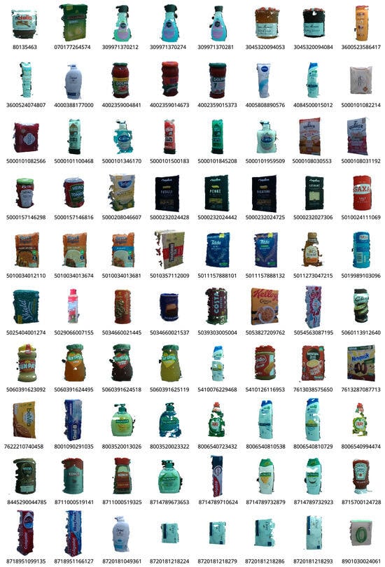
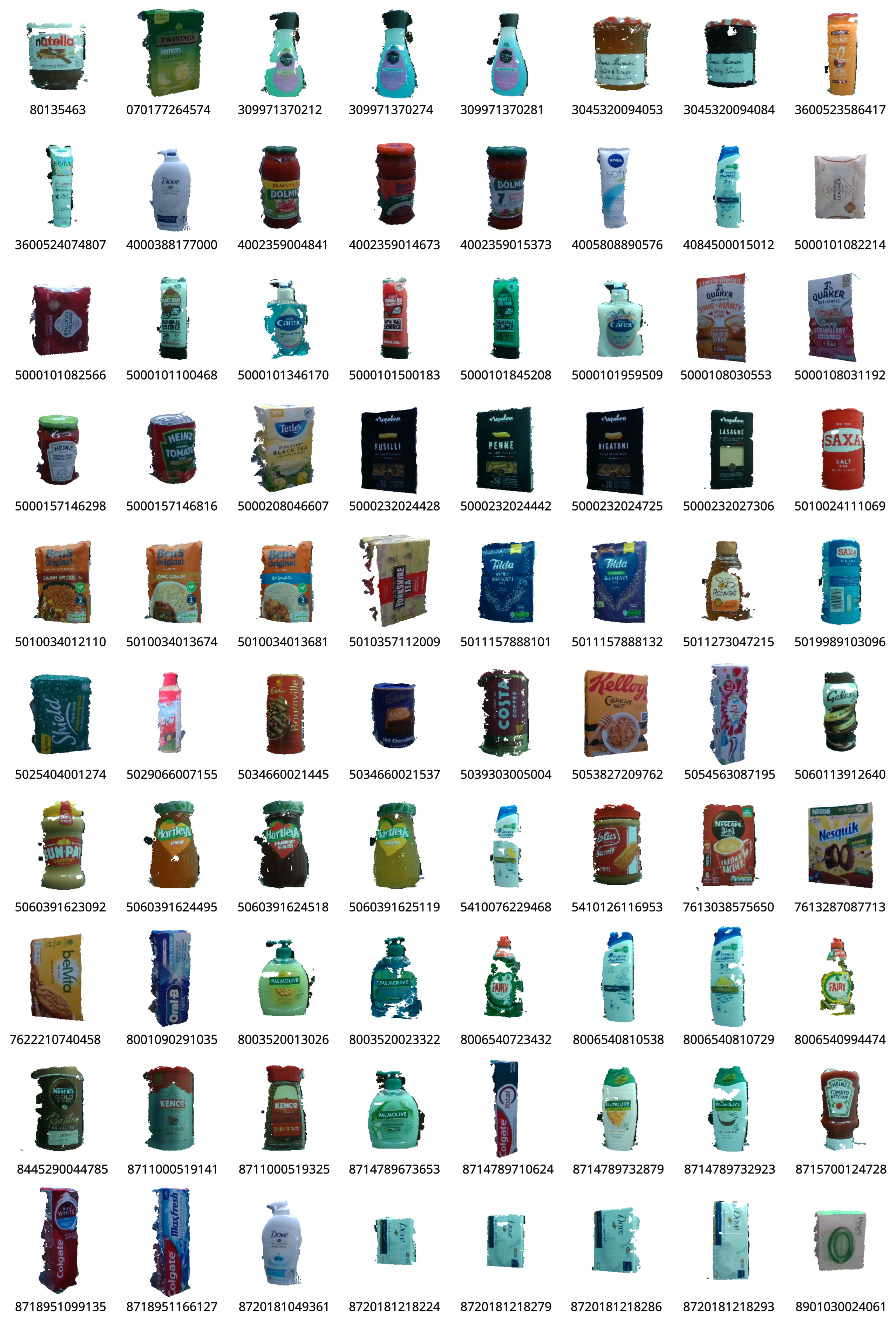
The MiniMarket80 dataset https://www.kaggle.com/datasets/mohamedsorour/minimarket80 (accessed on 26 December 2025) is made up of 1200 partial view samples per object for a total number of 80 objects. The grocery objects shown in Figure 1 and listed in Appendix A are chosen to span a range of sizes, textures and rigidities to serve as a low-cost, widely available benchmark dataset for point-cloud object segmentation in the context of robotic grasping. In the respective figure, these are named using their EAN (European Article Number) codes for higher reproducibility.

Figure 1. The MiniMarket80 dataset with each object’s EAN code.

Each view sample contains a number of colored points ranging from a few hundred to tens of thousands depending on the object’s visible features, RGB-D camera type, etc., and are publicly available in PCD (Point Cloud Data) format. The raw dataset is provided rather than a processed one for two reasons; firstly, to allow for arbitrary-resolution dataset generation based on the available processing power, and secondly, to facilitate dataset expansion, where only raw partial point cloud views for new bar-coded objects are needed (preferably 1200 unique views). Similarly, it would be straightforward to expand this dataset with scans of scenes containing multiple objects from the existing set, as we have done in this paper to provide test data for inference. In the following, we will present the collection setup and the processing necessary for the per-object segmentation dataset generation.

2.1. Collection Setup

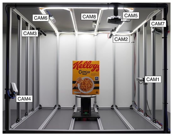
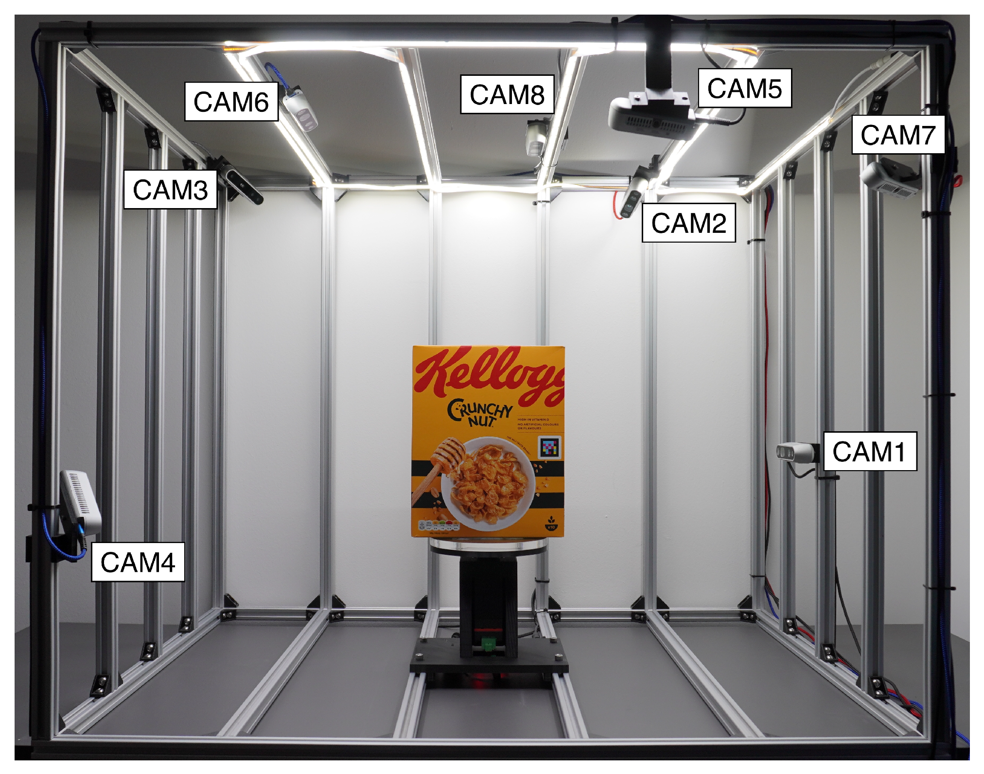
The dataset collection setup is shown in Figure 2, a video of which is available online (https://youtu.be/-Oes4mGOQhw) (accessed on 26 December 2025). The setup consists of 8 Realsense RGB-D cameras, 2 of which are D415, and the remaining 6 are D435. All of these are fitted in varying orientations facing a rotating table on which the object to be scanned is placed. The setup also features an LED array with controllable light intensity. As shown in the videos and in Figure 2, at each object pose, light intensity toggles between 3 values, and at each value, 8 partial views are captured. This gives a total of 24 partial views per object pose. The rotating table then rotates the object in 50 increments between 0° and 360°, giving rise to a total of 1200 partial view samples. Capturing the same view by each camera at 3 different light intensity values not only provides a robust training dataset against light variation but also against sensor noise. Also included in the dataset is a collection of 10 real-world multi-object scenes captured separately using a Realsense D415 camera and featuring a unique target object (EAN code 5410126116953) and a similar (in shape/color) distractor object (EAN code 503466002144) for the purpose of real-world inference testing.

Figure 2. Dataset collection setup.

2.2. Data Processing

The MiniMarket80 dataset is a collection of raw point cloud data with varying numbers of points. The pre-learning processing consists of two steps; a script for each is publicly provided (https://github.com/msorour/MiniMarket80) (accessed on 26 December 2025). In the first step, the raw 3D point cloud data is converted from PCD (Point Cloud Data) files into structured, fixed-size samples stored in HDF5 format; this is performed for each object dataset. While generating the fixed-size object dataset, the algorithm segments each large point cloud sample into smaller, uniform chunks with arbitrary size while preserving spatial relationships within each chunk, and it handles zero-padding for incomplete samples to maintain consistent sample dimensions. For example, if a raw object sample consists of 5 K points and a sample output of size 2048 points is required, the first 2048 points along the z-axis are packed into a first sample. The same goes for the second 2048 points, and a third sample is constructed from the final 904 points, zero-padded with the remaining 1144 points. Compared to random sampling, this methodology serves two purposes. First, it preserves spatial correlation between colored points (object texture), and second, it makes full use of all collected data.

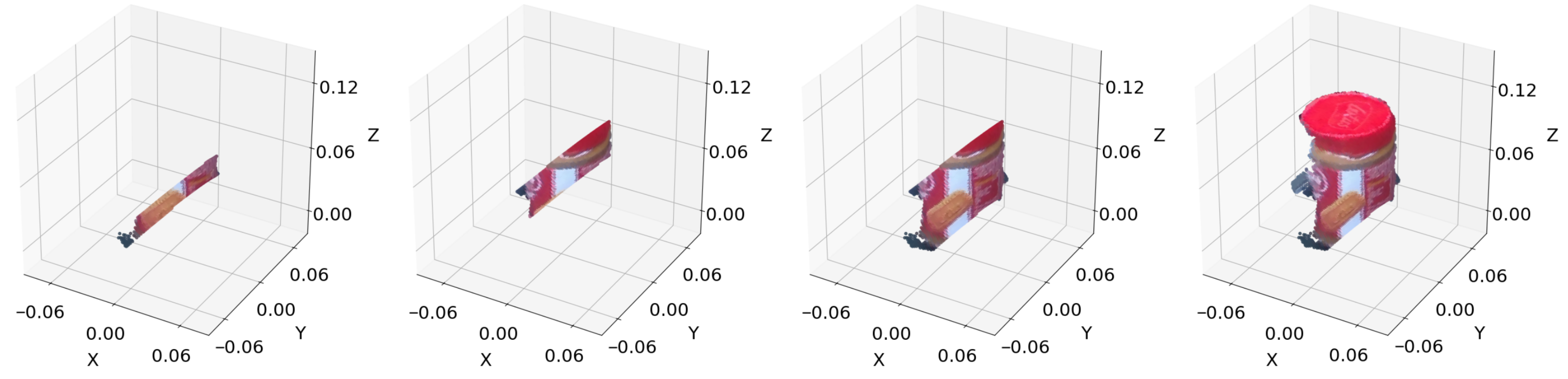
The output file consists of two primary HDF5 datasets: point cloud $(N\times P\times 3)$ storing $XYZ$ spatial coordinates and point cloud $(N\times P\times 3)$ storing corresponding $RGB$ color values, where N denotes the number of samples and P represents the number of points per sample. Both N and P are supplied to the algorithm to control the output—per object—dataset size depending on the available computation power and the number of points available in the raw PCD dataset. An example of varying numbers of points per object sample is shown in Figure 3, showing $P=1024$, 2048, 4096, and 8192, respectively, from left to right. It is evident that as the number of points per sample increases, more global features are present in a single sample at the expense of a very large object dataset. Whether or not this will enhance the “post-training” model performance will be examined below.

Figure 3. Examples of varying P (number of points per sample) with 1024, 2048, 4096, and 8192 points, respectively, from left to right.

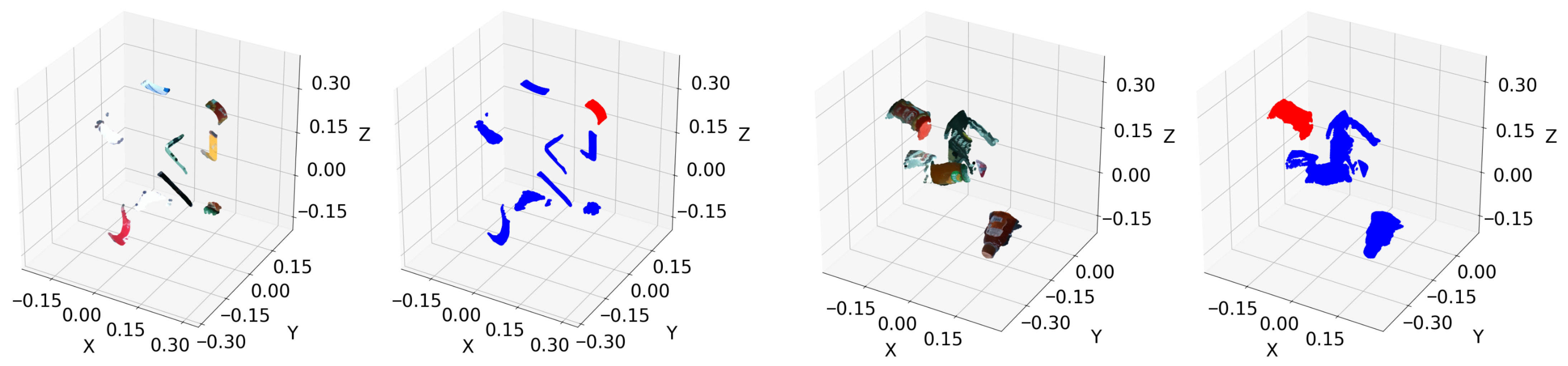
In a second step, a segmentation dataset is generated for a single unique target object by compositing the target samples with randomly selected “alien” objects under randomized spatial transformations, creating challenging training scenarios for unique item segmentation in point clouds; that is, the task of binary classification of the points belonging to a specific object among distractors. For each sample, it applies randomly generated rigid transformations—rotations (0–180°) and translations—to both target and alien objects, ensuring non-overlapping configurations through constrained spatial sampling. The output HDF5 structure contains three datasets: point cloud $(N\times P\times 3)$ for 3D coordinates, point cloud $(N\times P\times 3)$ for RGB values, and segmentation labels (or segmentation mask) $(N\times P\times 2)$ for one-hot encoded labels distinguishing target ([1, 0]), alien ([0, 1]), and padding ([0, 0]) points. The methodology introduces controlled variability by allowing 0 to k alien objects per sample (k configurable) and incorporating a user-defined percentage of negative samples (target absent). Two training segmentation samples are depicted in Figure 4; each sample is a pair of input colored point cloud and output segmentation mask (colored in red and blue, designating the target and alien objects, respectively). The sample pair to the (left) and (right) of the respective figure are constructed from object datasets generated with 2048 and 8192 points per object sample, respectively, giving rise to a segmentation sample of 20,480 and 81,920 points for a 10-object sample.

Figure 4. Examples of two segmentation sample pairs (sample and mask), with 20,480 points (left) and 81,920 points (right). The target and alien objects are colored in red and blue respectively in the segmentation mask.

2.3. Experiments and Methodology

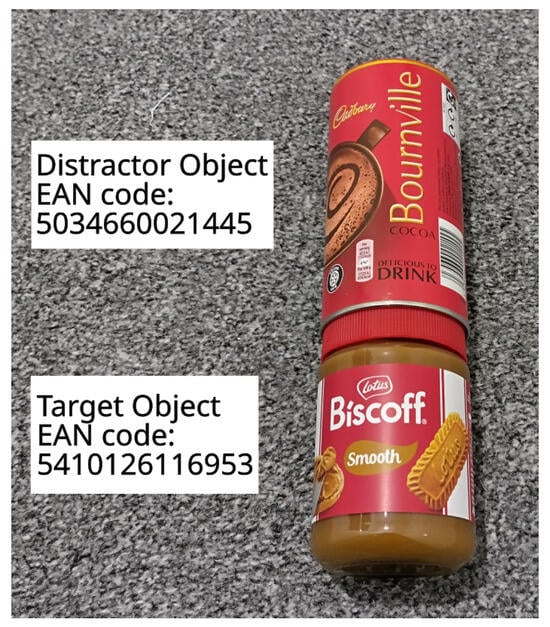
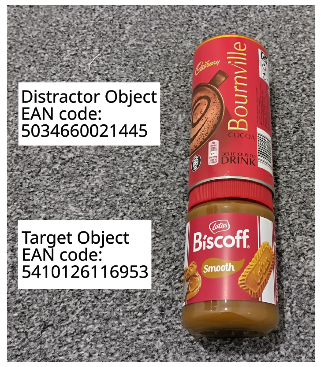
In the first experiment, a collection of 11 state-of-the-art segmentation networks (briefly described in the following) are adapted to accept 6D colored point coordinates as well as binary segmentation score output for the two classes: target or alien. These are then trained on our dataset, aiming at unique object segmentation. In this initial experiment, we use a segmentation dataset with 2048 points per object sample. An example of such sample is depicted in Figure 4 left, where the target object has the EAN code 5410126116953. The inference of each trained model will be performed on an arbitrary real-world scene among 10 supplied in the dataset designed to have several alien objects. One of these is designated as the distractor object 5034660021445, characterized by similar geometry (cylindrical), dimension and overall color as the target object, as shown in Figure 5. This is to test if a particular trained network architecture can recognize the object texture and features rather than just general shape and color. To facilitate future reference to this benchmark, we have termed this experiment “binary Segmentation of Unique Object among Distractor Objects” (SUODO_20480) with the appended numeral representing the segmentation sample size. In the second experiment, the best-performing architectures are trained using a segmentation dataset with 8192 points per object sample (SUODO_81920) (an example of such sample is depicted in Figure 4 right) to check if increasing the sample size can improve training and to compare the architecture inference results on all real-world scenes.

Figure 5. Target and distractor objects.

The segmentation network architectures are chosen to cover a range of methods, including point-based, graph, convolution, and transformer-based methods. These are also picked to fit practical hardware constraints, namely plausibility for training on a single RTX3090 GPU. In the following, we will describe these in brief starting with the pioneering baseline model, PointNet [47], presenting a breakthrough in direct point cloud processing by introducing a network architecture that consumes unordered point sets without requiring voxelization or projection. It achieves permutation invariance through symmetric functions, enabling robust processing of unordered point clouds. Shared multi-layer perceptrons (MLPs) independently map each point to a high-dimensional feature space, followed by symmetric max-pooling to aggregate a global feature vector. An input transformation network (T-Net) canonicalizes point sets via an affine matrix, ensuring invariance to rigid transformations. This design makes the network’s output a function of the overall set rather than point order. For segmentation, the architecture concatenates the global feature with point-wise local features from intermediate layers. The resulting enriched vectors are processed by subsequent MLPs to assign semantic labels per point, integrating both global shape context and local geometric details.

The PointNet architecture is further enhanced in PointNet++ [48] by introducing a hierarchical architecture that enables robust learning of local features at multiple scales. This is constructed through a series of set abstraction layers, each of which progressively subsamples the point cloud, groups points into local regions, and applies a mini-PointNet to extract features from these groups. To handle non-uniform point densities commonly found in real-world data, PointNet++ incorporates novel sampling and grouping layers via two key strategies, namely Multi-Scale Grouping and Multi-Resolution Grouping. By systematically capturing local features, PointNet++ achieves significantly greater generalization and accuracy compared to its predecessor.

Subsequent point-based architectures focused on efficiency and local feature extraction. RandLANet [49] prioritized scalability for large scenes by employing random sampling and a local feature aggregation module with attentive pooling, bypassing the computational cost of iterative farthest point sampling. PointWeb [50] introduced dense inter-point connections within local patches via its Adaptive Feature Adjustment (AFA) module, creating a rich web for feature context exchange between all points in a neighborhood. In a complementary approach, PointMLP [51] demonstrated that state-of-the-art performance could be achieved with a simpler approach, using a series of residual MLPs augmented with geometric affine transformations for deep feature refinement, proving that sophisticated local feature extraction modules are not always necessary.

PointNext [52] enhances the PointNet++ architecture by optimizing its core components and training strategies. The framework introduces an Inverted Residual MLP block, which incorporates residual connections to aid training, separable MLPs for computational efficiency, and an inverted bottleneck design to enrich features. These are complemented by architectural changes, including a unified deeper encoder, a symmetric decoder, and an initial stem MLP, collectively enabling effective and efficient model scaling. In [53], the PointeNet architecture introduced a lightweight framework that effectively captures comprehensive point cloud features by combining non-learnable components with minimal learnable parameters. Its core innovations are the Multivariate Geometric Encoding (MGE) module, which uses sampling, grouping, and pooling operations to adaptively aggregate diverse 3D geometric features (spatial, curvature, normal), and the Distance-aware Semantic Enhancement (DSE) module, which introduces a distance-aware factor into semantic segmentation to enhance perception for distant points for autonomous driving scenarios. This design claims to achieve state-of-the-art performance on object-level and scene-level tasks with significantly fewer parameters and lower computational cost.

Significant research efforts aim to adapt successful 2D convolution networks for point cloud processing. PointCNN [54] introduced the seminal $\chi$-Transformation, which learns a canonical ordering and weighting of points in a local region. This transformation effectively convolves over the features of neighboring points, allowing for the application of a standard convolution operator on the now-ordered set. DGCNN [55] instead constructs a dynamic graph in the feature space at each layer, connecting points to their k-nearest neighbors. Its core operator, EdgeConv, applies a convolution-like operation on the edges of this graph, aggregating features from a point’s neighbors.

The significant success achieved by the transformer self-attention [56] mechanisms in machine translation has motivated substantial research efforts to adapt these architectures for point cloud segmentation. Transformer-based approaches abandon pooling and convolution in favor of the self-attention mechanism to define local neighborhoods. Point Transformer [57], for example, replaces the symmetric aggregation function in PointNet++ or the edge convolution in DGCNN with a transformer block that computes self-attention within a local point set. Building on this, the Fast Point Transformer [58] addresses the computational bottleneck of applying self-attention to large point clouds by introducing a novel architecture that uses voxel-based hashing to efficiently group points and compute self-attention only within these local, spatially coherent groups. Further advancing this trend, Point Transformer V3 [59] diverges from its predecessor by replacing the computationally intensive vector self-attention with a much simpler, yet highly effective, grouped linear attention mechanism, which dramatically reduces the operational complexity.

3. Results

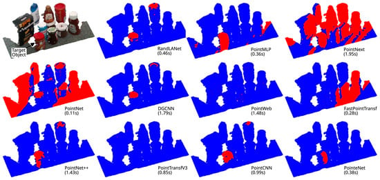
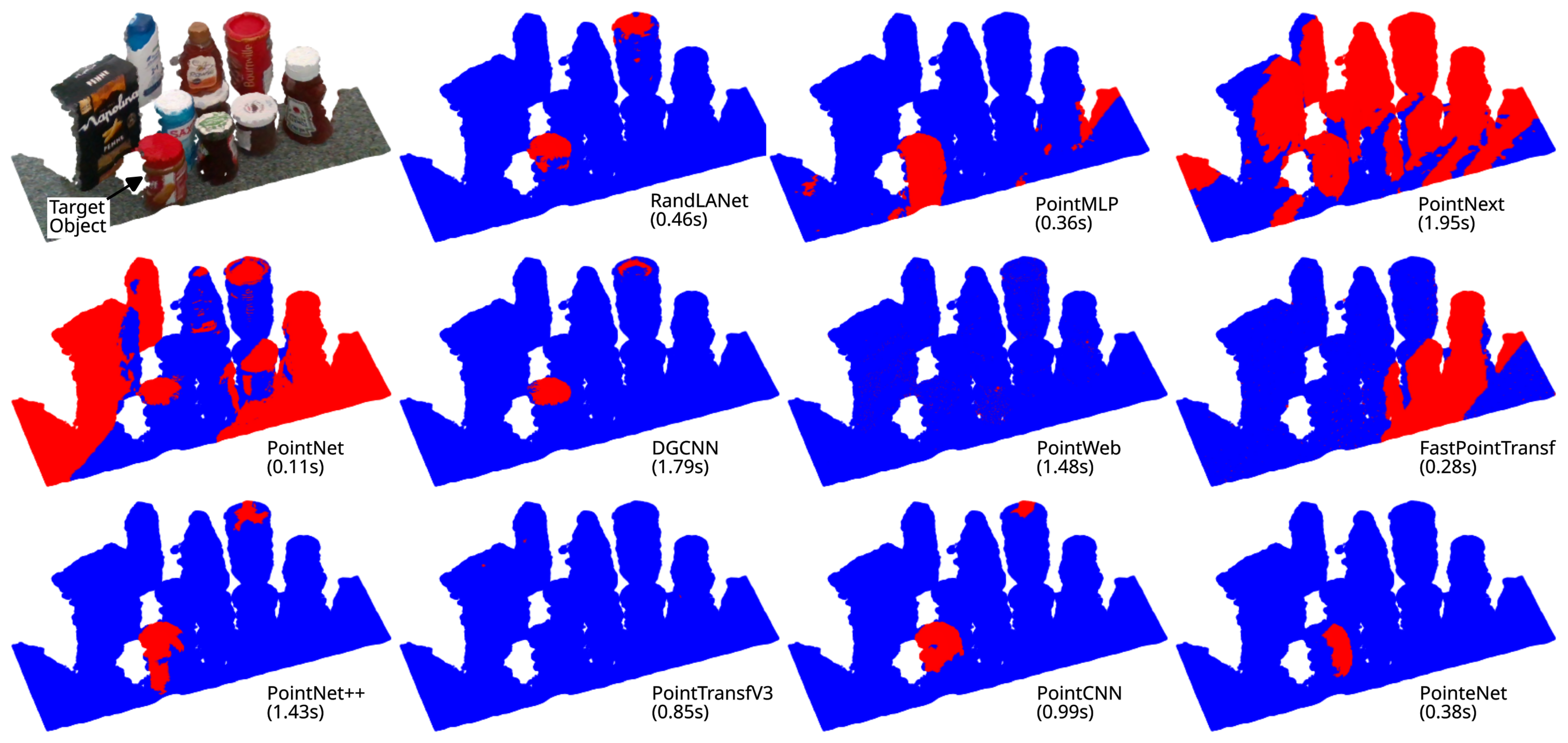
In a first benchmark SUODO_20480, the segmentation methods described in the previous section are adapted and trained on our dataset, where default architecture configuration and parameter settings are used. Details of each network model and training parameters are provided in Appendix B, and training results are listed in Table 2, arranged in ascending order of the mean Intersection Over Union (mIOU) obtained in validation. In this experiment, the segmentation datasets for training were generated with a size of 20,480 colored points consisting of object samples with 2048 points each. A sample of such dataset is shown in Figure 4 left. The inference result of each of the 11 methods on a real-world scene (supplied with the dataset) is depicted in Figure 6.

Table 2. Training duration and results of the first experiment.

Method	Parameter Count (M)	Training Time per Epoch (s)	Best Valid mIOU (%)	Best Epoch/Total
PointWeb	0.98	583	71.3	55/75
FastPointTransf	36	495	75.8	04/25
PointNext	17.6	1367	81.2	121/175
PointTransfV3	31.7	531	81.4	48/75
RandLANet	1.3	2800	83.9	09/50
DGCNN	1.28	1974	85.3	54/75
PointNet	3.5	167	86.9	11/150
PointCNN	1.45	1004	92.7	03/25
PointNet++	0.97	356	93.7	32/75
PointMLP	15.3	189	98.1	46/50
PointeNet	8.68	187	99.7	50/50

Figure 6. Inference results of the first experiment on real-world scene 7 with number of points = 200,715. Predictions of target and alien objects are colored in red and blue respectively.

It is important to note that the presented inference results are based on real-world experiments, not on synthetic validation data. The number of points in this particular scene is 200,715 and the inference time is shown per network architecture. Although we lack ground truth for the real-world scene, it is readily apparent to what extent each method is able to segment the target object without misclassification of alien objects including the distractor.

As illustrated in Figure 6, only four methods—PointeNet, PointCNN, PointNet++, and PointMLP—successfully learned to capture unique object features, including both shape and texture. This can be eye-judged in the respective figure, where the segmented target object and aliens are colored in red and blue, respectively. An ideal segmentation result would show only the target object (labeled in the top-left image of Figure 6) colored red with all other points in blue. However, PointMLP and PointeNet produced significant false positives and negatives, respectively, for such a high mIOU validation result. It is worth pointing out that a false negative where the correct object is partially segmented has less severe consequences compared to false positives where alien objects are mistakenly identified as the target.

In contrast, PointNet, PointNeXt, PointWeb, and the transformer-based models failed to train on our dataset, where from the inference results in Figure 6, it is evident these were not able to distinguish the target object or aliens. Meanwhile, RandLA-Net and DGCNN managed to learn some distinguishing features and were not confused by alien objects, yet these did not capture unique object textures, as evident by just segmenting the circular red cap in both the object and the distractor, but none of the side texture of the target. The best-performing methods are then used in a second experiment to be trained on a higher-resolution segmentation dataset with a sample size of 81,920 points consisting of object samples with 8192 points each; an example of such sample is shown in Figure 4 right. The rationale for this experiment stems from the inference process: applying a model trained on x points per sample necessitates dividing a scene point cloud into segments of x points. Consequently, increasing the training sample size reduces the number of segments, leading to fewer iterative inferences and a shorter total inference duration.

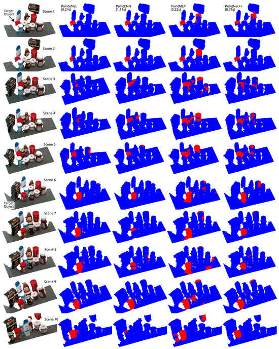
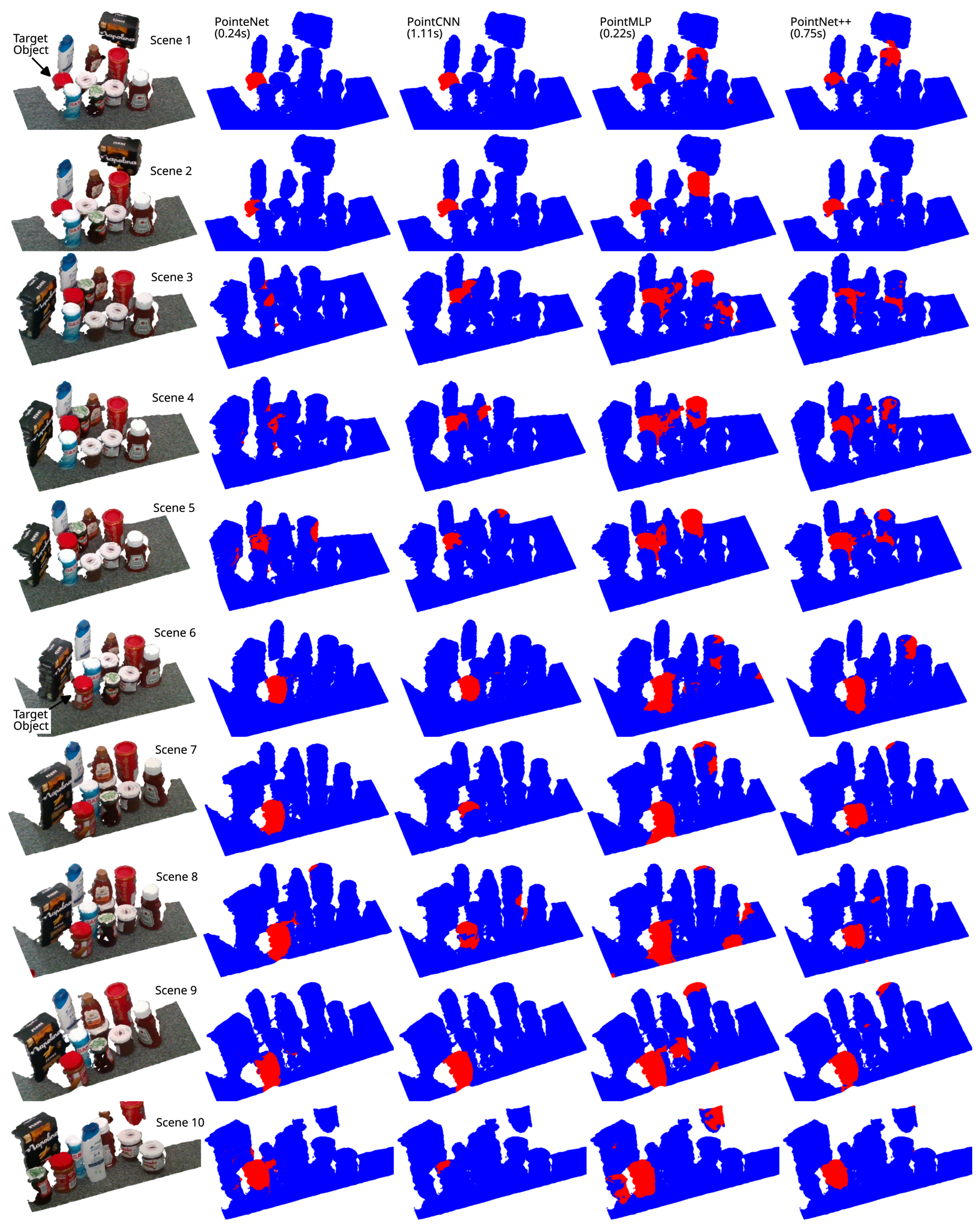
The training and inference results for the second benchmark experiment SUODO_81920 are shown in Figure 7 and Table 3 for the 10 real-world scenes, respectively. As shown, PointeNet performed reasonably well compared to the other methods, specially when the target object’s unique texture is visible, as was the case in scenes 6 to 10. The inference time improved by 1.78 times as well from 0.38 s for 200,715 points in the first experiment (1.893 s per million points) to an average of 0.24 s for 225,852 points in the second experiment (1.062 s per million points).

Figure 7. Inference results of the second experiment on 10 real-world scenes, with an average 225,852 points per scene. Predictions of target and alien objects are colored in red and blue respectively.

Table 3. Training duration and results of the second experiment.

Method	Parameter Count (M)	Training Time per Epoch (s)	Best Valid mIOU (%)	Best Epoch/Total
PointNet++	0.97	1228	94.5	64/100
PointCNN	1.45	3815	95.9	32/100
PointMLP	15.3	527	97.4	89/100
PointeNet	8.68	632	99.4	81/100

The inference results also appear to improve with the larger segmentation sample (e.g., comparing scene 7 of the second experiment in Figure 7 to the first experiment in Figure 6), likely because these training samples preserve more of the spatial and texture relationships unique to the target object.

4. Discussion

The evaluation of 3D deep learning architectures is largely dependent on a standardized suite of benchmark datasets. Typical benchmarks include ModelNet40 for object classification, ShapeNetPart for part segmentation, and S3DIS [45], ScanNet, and SemanticKITTI [46] for indoor and outdoor semantic segmentation, respectively. A significant limitation of these datasets is their predominant focus on textureless objects and scenes, which does not adequately assess a model’s capability for recognizing unique, textured items. Consequently, architectures tested primarily on these benchmarks may not generalize well to real-world applications requiring fine-grained texture discrimination, as tested in the current work.

For instance, Point Transformer V3 and Fast Point Transformer were previously evaluated on indoor scene segmentation (ScanNet), achieving mIOUs of 78.6% and 72.1%, respectively, with voxel grid sizes of 0.005 and 0.02 mm. Their relatively poor performance on textured real-world data, as shown in Figure 6, aligns with this benchmark limitation. Similarly, PointNeXt and PointWeb achieved their best reported mIOUs on S3DIS (6-fold) at 74.9% and 66.7%, respectively, while attaining higher mAcc scores of 90.8% and 89.4%. This disparity suggests these models are more optimized for geometric shape learning than for texture reasoning, further underscored by the absence of their evaluation on part segmentation benchmarks like ShapeNetPart.

In contrast, architectures such as PointeNet, PointCNN, PointMLP, DGCNN, and PointNet++ have been validated on ShapeNetPart for part segmentation, reporting instance segmentation mIOUs of 85.6%, 84.6%, 85.7%, 85.2%, and 85.1%, respectively. A general trend emerges: models that perform well on the shape-oriented ShapeNetPart benchmark also demonstrate reasonable efficacy on our segmentation dataset, which involves greater texture variability. This further highlights the need for benchmarks that incorporate textured data to comprehensively evaluate model capabilities.

The PointeNet architecture demonstrated superior performance in the second experiment (Figure 7), establishing it as the optimal baseline for future development due to its balance of accuracy and computational efficiency. This effectiveness stems from its Multivariate Geometric Encoding (MGE) module, which integrates Farthest Point Sampling (FPS) and k-Nearest Neighbors (k-NN) with a core Multivariate Local Geometric Aggregation (MLGA) component. The MLGA module directly encodes critical surface properties, such as curvature and normals, alongside spatial relationships through position encoding and adaptive aggregation. This design enables the capture of rich geometric information with notably low computational overhead compared to more complex fusion strategies.

Alternative methods, PointCNN and PointNet++, also performed competitively, occasionally surpassing PointeNet in specific segmentation scenes (2–4). On the one hand, PointCNN adapts convolutional principles to point clouds via its core $\chi$-Conv operator. This operation first achieves translation invariance by transforming neighboring points into a local coordinate system. It then lifts these coordinates into a higher-dimensional feature space using an MLP, concatenates them with existing features, and applies a learned $\chi$-transformation matrix to weight and order the data before final convolution. This process systematically aggregates local neighborhood information into richer features for representative points. On the other hand, PointNet++ employs a hierarchical framework to capture multi-scale context. Its iterative Set Abstraction layers first use FPS to select centroid points, then they group neighboring points via a ball query. A core innovation is its multi-scale grouping (MSG) strategy, which enhances robustness to varying point densities and scales. Instead of using a single radius for the ball query grouping operation, MSG simultaneously extracts features from the same centroid point using multiple radii, capturing local patterns at different spatial scales. Each local neighborhood is processed by a shared MLP—acting as a localized PointNet—to generate a single feature vector encoding that region’s geometry. Through recursion, these local features are progressively aggregated, allowing the network to build increasingly complex representations from local patterns to global structure. We suggest that combining local feature aggregation approaches from PointeNet’s MGE, PointCNN’s $\chi$-Conv operator, and PointNet++ MSG could yield a more robust feature extraction framework and superior segmentation performance. Although the four network architectures demonstrated superior performance (among the limited pool of networks tested) and achieved high optimization values (Table 3), their real-world testing results (Figure 7) exhibited clear segmentation errors. The varying magnitude of these errors, as visually assessed, indicates that the architectures differ in their ability to capture local object features, with some—particularly PointMLP—potentially overfitting.

Inference speed is a critical performance metric. Among the 11 methods evaluated, PointeNet achieved a competitive inference throughput of 1.062 s per million points. For context, this rate must increase by a factor of at least 31 to match the real-time data output of a RealSense D415 RGB-D camera (approximately 1 million points at 30 Hz). On the one hand, it is important to note that the reported benchmark was conducted in a pure Python environment on an RTX 3090 GPU. Significant acceleration is anticipated by porting the model to a C/C++ implementation and utilizing more recent GPU hardware. On the other hand, a comparison of the inference results—specifically from scene 7 of the second experiment in Figure 7 with those from the first experiment in Figure 6—allows us to generally conclude that increasing the size of the segmentation sample consequently increases the object features per sample, yielding better results. These improvements were observed both in terms of inference accuracy and speed. However, due to constraints on the available GPU hardware, we were not able to investigate this relationship further for potential inference time efficiency gains. This limitation, alongside model and implementation enhancements, constitutes part of our motivation for future work.

It should be noted that the real-world inference experiments, although conducted using real scenarios, may not fully capture the complexities associated with densely packed shelves or containers in practical deployments. As such, the current real-world validation dataset serves as a preliminary benchmark for evaluating state-of-the-art network architectures. Future work will involve expanding these validation scenes and providing comprehensive annotations for the various objects to enable quantitative evaluation of segmentation performance. This would also make possible a more detailed analysis of the relative contribution to success of specific components in the pipeline, such as inclusion of scans with varied lighting or noise-filtering thresholds for the Realsense cameras. In addition, the methods for generating synthetic scenes with multiple objects for training could be further adapted to be consistent with specific real-world scenarios.

5. Conclusions

In this work, we presented the MiniMarket80 dataset to address a gap in the availability of suitable training and evaluation data for unique item segmentation from point cloud data. Existing 3D object grasping datasets are mostly CAD based and grasp planning oriented, while datasets benchmarking point cloud segmentation methods are mostly textureless. In contrast, the MiniMarket80 dataset provides multiple RGB-D scans, under varying viewpoints and lighting conditions, of easily procured standard objects to enhance reproducibility. A pipeline for generating a per-object segmentation dataset is presented and used to train 11 existing segmentation methods, tested against real-world multi-object scenes. The results suggest that those segmentation methods reportedly performing well on the ShapeNetPart benchmark are more likely to capture unique texture-rich local features in our dataset, but they also indicate substantial need for improvement of these methods to obtain robust performance.

Appendix B.1. PointNet

• Network Architecture:

• Spatial Transformer Networks (T-nets):

  –

  Input T-net: $6\to 64\to 128\to 1024\to 512\to 256\to 36$ (output: $6\times 6$ transformation matrix)

  –

  Feature T-net: $64\to 128\to 1024\to 512\to 256\to 4096$ (output: $64\times 64$ transformation matrix)

  –

  Each layer: Batch normalization + ReLU activation

  –

  Max pooling over all points before fully connected layers

• PointNet Backbone:

  –

  Input transformation via T-net (3D coordinates + RGB features)

  –

  First shared MLP: $6\to 64\to 64$ (implemented as $1\times 1$ convolutions)

  –

  Feature transformation via T-net ($64\times 64$)

  –

  Second shared MLP: $64\to 64\to 128\to 1024$ ($1\times 1$ convolutions)

  –

  Global feature extraction via max pooling over all points

  –

  Local features (64-dim) concatenated with global features (1024-dim) for segmentation

• Heads:

  –

  Classification: $1024\to 512\to 256\to k$ classes

  *

  Batch normalization in first two layers

  *

  Dropout ($p=0.3$) before final layer

  –

  Segmentation: $1088\to 512\to 256\to 128\to m$ classes

  *

  Batch normalization in first three layers

  *

  No dropout

• Training Parameters:

• Optimization:

  –

  Optimizer: Adam with learning rate $0.001$, weight decay $1\times {10}^{-4}$

  –

  Scheduler: CyclicLR with $\mathrm{base}\text{\_}\mathrm{lr}=0.0001$, $\max \text{\_}\mathrm{lr}=0.01$, $\mathrm{step}\text{\_}\mathrm{size}\text{\_}\mathrm{up}=2000$

• Loss Functions:

  –

  Segmentation: Balanced Cross-Entropy with focal modulation ($\gamma =1$) + Dice loss

  –

  Orthogonal regularization weight: $0.001$ (for feature transformation matrix)

Appendix B.2. PointNet++

• Network Architecture:

• Set Abstraction Layers:

  –

  SA1: 1024 points, radius = 0.01, 32 neighbors

  –

  SA2: 256 points, radius = 0.05, 32 neighbors

  –

  SA3: 64 points, radius = 0.2, 32 neighbors

  –

  SA4: 16 points, radius = 0.3, 32 neighbors

  –

  MLP configurations: SA1: $[32,32,64]$, SA2: $[64,64,128]$, SA3: $[128,128,256]$, SA4: $[256,256,512]$ channels

• Feature Propagation Layers:

  –

  FP4: $768\to 256\to 256$ channels

  –

  FP3: $384\to 256\to 256$ channels

  –

  FP2: $320\to 256\to 128$ channels

  –

  FP1: $128\to 128\to 128\to 128$ channels

• Input Representation:

  –

  Farthest point sampling for point selection

  –

  Ball query with radius-based grouping

• Training Parameters:

• Optimization:

  –

  Optimizer: Adam with learning rate $0.001$, weight decay $1\times {10}^{-4}$

  –

  Scheduler: CyclicLR with $\mathrm{base}\text{\_}\mathrm{lr}=0.0001$, $\max \text{\_}\mathrm{lr}=0.01$, $\mathrm{step}\text{\_}\mathrm{size}\text{\_}\mathrm{up}=2000$

  –

  Gradient clipping: $\max \text{\_}\mathrm{norm}=1.0$

• Loss Function: Focal loss ($\gamma =1$) + Dice loss
• Regularization:

  –

  Batch normalization after each convolutional layer

  –

  Dropout ($p=0.5$) before final classification layer

  –

  Weight decay ($L_2$ regularization) coefficient $1\times {10}^{-4}$

Appendix B.3. RandLA-Net

• Network Architecture:

• Local Feature Aggregation (LFA) Modules:

  –

  4 hierarchical LFA layers (encoder) with feature dimensions: $(8\to 16\to 64\to 128\to 256)$

  –

  Neighborhood search: K-nearest neighbors with $K=16$

  –

  Local Spatial Encoding (LSE): 10-dimensional spatial encoding

  –

  Attentive pooling with learned importance scores

• Architecture Structure:

  –

  Encoder–decoder with 4 encoding and 4 decoding layers

  –

  Decimation factor: $4\times$ point reduction per encoding level

  –

  4 upsampling layers (decoder) (512 → 256 → 128 → 32 → 8)

  –

  Skip connections between encoder and decoder layers

  –

  Output layer: MLP $(8\to 64\to 32\to \mathrm{num}\text{\_}\mathrm{classes})$ with dropout

• Training Parameters:

• Optimization:

  –

  Optimizer: Adam with learning rate $0.001$, weight decay $1\times {10}^{-4}$

  –

  Scheduler: CyclicLR with $\mathrm{base}\text{\_}\mathrm{lr}=0.0001$, $\max \text{\_}\mathrm{lr}=0.01$, $\mathrm{step}\text{\_}\mathrm{size}\text{\_}\mathrm{up}=2000$

  –

  Gradient clipping: $L_2$ norm clipping with $\max \text{\_}\mathrm{norm}=1.0$

• Loss Function: Focal loss ($\gamma =1$) + Dice loss
• Regularization:

  –

  Batch normalization ($ϵ=1\times {10}^{-6}$, momentum = 0.99)

  –

  Dropout

Appendix B.4. PointWeb

• Network Architecture:

• Core Components:

  –

  Adaptive Feature Adjustment (AFA) Module: Learns point-wise relationships

  –

  Hierarchical Set Abstraction that progressively down-samples the point cloud with 4 SA modules

  –

  4 Feature Propagation modules that up-sample features back to original resolution

• Set Abstraction Layers:

  –

  SA1: 1024 points, 32 neighbors, MLP $[C,32,32,64]$, AFA MLP $[16,16]$

  –

  SA2: 256 points, 32 neighbors, MLP $[64,64,64,128]$, AFA MLP $[16,16]$

  –

  SA3: 64 points, 32 neighbors, MLP $[128,128,128,256]$, AFA MLP $[16,16]$

  –

  SA4: 16 points, 32 neighbors, MLP $[256,256,256,512]$, AFA MLP $[16,16]$

• Feature Propagation (FP) Modules:

  –

  FP1: MLP $[128+C,128,128,128]$, C denotes feature channels

  –

  FP2: MLP $[256+64,256,128]$

  –

  FP3: MLP $[256+128,256,256]$

  –

  FP4: MLP $[512+256,256,256]$

• Key Features:

  –

  Farthest Point Sampling (FPS) for point selection

  –

  K-Nearest Neighbors (KNN) with $k=32$

  –

  Shared MLPs as 2D convolutions

  –

  Max pooling for local feature aggregation

  –

  Skip connections between SA and FP modules

• Training Parameters:

• Optimization:

  –

  Optimizer: Adam with weight decay $1\times {10}^{-4}$, learning rate $0.001$

  –

  Scheduler: StepLR with step size = 20 epochs, $\gamma =0.5$

  –

  Gradient clipping: $L_2$ norm clipping with $\max \text{\_}\mathrm{norm}=1.0$

• Loss Function: Focal loss ($\gamma =2$) + Dice loss + Cross-entropy with class weighting
• Regularization:

  –

  Batch normalization on all convolutional layers

  –

  Dropout in final classification layer

  –

  Weight decay coefficient $1\times {10}^{-4}$

Appendix B.5. PointCNN

• Network Architecture:

• Core Components:

  –

  X-Convolution: Convolution on X-transformed points

  –

  X-Transformation Matrix: Learned $K\times K$ matrix

  –

  Hierarchical encoder–decoder structure

• Encoder Configuration:

  –

  Multiple RandPointCNN layers that progressively downsample the point cloud

  –

  Each layer applies X-Convolution (core operation of PointCNN)

  –

  Layer 1: 64 output channels, 8 neighbors, dilation 1, 1024 representative points

  –

  Layer 2: 128 output channels, 12 neighbors, dilation 2, 512 points

  –

  Layer 3: 256 output channels, 16 neighbors, dilation 2, 128 points

  –

  Layer 4: 512 output channels, 16 neighbors, dilation 3, 32 points

• Decoder Configuration:

  –

  Multiple PointCNN layers that upsample features back to original resolution

  –

  Uses skip connections from encoder layers

  –

  Layer 1: 256 output channels, 16 neighbors, dilation 2, 128 points

  –

  Layer 2: 128 output channels, 12 neighbors, dilation 2, 512 points

  –

  Layer 3: 128 output channels, 8 neighbors, dilation 1, 1024 points

• Key Features:

  –

  Depthwise separable convolutions

  –

  Farthest Point Sampling (FPS)

  –

  K-Nearest Neighbors (KNN) with dilation factor D

  –

  Inverse distance weighting for upsampling

  –

  Skip connections

• Segmentation Head: Dense(128) → Dropout(0.5) → Dense(num_classes)

• Training Parameters:

• Loss Function: Combined focal loss ($\gamma =2.0$) and Dice loss
• Optimizer: Adam with weight decay $1\times {10}^{-4}$, initial lr = 0.001
• Scheduler Options: StepLR
• Gradient Clipping: Max norm 1.0
• Regularization: Batch normalization (momentum = 0.9), Dropout (0.5)

Appendix B.6. PointMLP

• Network Architecture:

• Encoder Components:

  –

  Initial embedding: 1D convolution with 64 output channels

  –

  Four hierarchical stages with downsampling factors $[4,4,4,4]$

  –

  Each stage: LocalGrouper (FPS + KNN, $K=32$) + PreExtraction + PosExtraction

  –

  Channel dimensions: $[64,128,256,512]$ (expansion factor of 2 per stage)

  –

  Anchor-based normalization with learnable parameters

• Decoder Components:

  –

  Three upsampling stages: $[512,256,128]$ channels

  –

  Each decoder stage: 2 residual blocks

  –

  Skip connections from encoder

• Classification Head:

  –

  Global context via multi-scale max pooling

  –

  Class token integration (16-dimensional)

  –

  Final classifier: 128-channel hidden layer with dropout → output layer

Training Parameters:

• Optimization:

  –

  Optimizer: Adam with weight decay $1\times {10}^{-4}$, lr = 0.001

  –

  Scheduler: CyclicLR ($\mathrm{base}\text{\_}\mathrm{lr}=0.0001$, $\max \text{\_}\mathrm{lr}=0.01$, $\mathrm{step}\text{\_}\mathrm{size}\text{\_}\mathrm{up}=2000$)

  –

  Gradient clipping: Max norm 1.0

• Loss Function: Focal loss ($\gamma =2$) + Dice loss + Cross-entropy
• Regularization: Batch normalization, Dropout, Weight decay

Appendix B.7. DGCNN

• Network Architecture:

• Graph Construction:

  –

  K-nearest neighbors graph with $k=20$ neighbors per point

  –

  Edge features: concatenation of relative coordinate differences + original features

  –

  Dynamic graph updating at each layer

• Feature Extraction:

  –

  Four EdgeConv layers: $64\to 64\to 128\to 256$ channels

  –

  Each EdgeConv: 2D convolution ($1\times 1$) + BatchNorm + LeakyReLU (slope = 0.2)

  –

  Max pooling after each EdgeConv

  –

  Feature concatenation across layers

• Embedding Layer:

  –

  1D convolution: 512 → 1024 channels

  –

  BatchNorm + LeakyReLU

• Segmentation Head:

  –

  Sequential 1D convolutions: $1024\to 512\to 256\to$ num_classes

  –

  BatchNorm + LeakyReLU in first two layers

  –

  No activation on final layer

• Training Parameters:

• Optimization:

  –

  Optimizer: Adam (lr = 0.001)

  –

  Weight decay: $1\times {10}^{-4}$

  –

  Scheduler: CyclicLR ($\mathrm{base}\text{\_}\mathrm{lr}=0.0001$, $\max \text{\_}\mathrm{lr}=0.01$)

  –

  Gradient clipping: max norm=1.0

• Loss Function: Focal loss ($\gamma =1$) + Dice loss + Cross-entropy with class weighting

Appendix B.8. Point Transformer V3

• Network Architecture:

• Core Architecture:

  –

  Serialized attention with Z-order and Hilbert curve encoding

  –

  Encoder–decoder with skip connections

• Encoder Configuration:

  –

  4-stage hierarchical encoder with depths: $(2,2,2,2)$ transformer blocks

  –

  Channel dimensions: $(64,128,256,512)$

  –

  Multi-head attention heads: $(2,4,8,16)$ per stage

  –

  Patch sizes: $(2048,1024,512,256)$

  –

  Strided downsampling factors: $(2,2,2)$

• Decoder Configuration:

  –

  3-stage decoder with depths: $(1,1,1)$ transformer blocks

  –

  Channel dimensions: $(256,128,64)$

  –

  Multi-head attention heads: $(8,4,2)$ per stage

  –

  Patch sizes: $(512,1024,2048)$

  –

  Serialized unpooling with skip connections

• Attention Mechanism:

  –

  Serialized attention with spatial ordering

  –

  Scaled dot-product attention

• Normalization and Activation:

  –

  Pre-normalization with LayerNorm in attention blocks

  –

  GroupNorm (32 groups) in convolutional layers

  –

  GELU activation

  –

  Stochastic depth with drop path rate 0.01

• Training Parameters:

• Optimization:

  –

  Optimizer: Adam with lr = 0.001, weight decay $1\times {10}^{-4}$

  –

  Scheduler: CyclicLR ($\mathrm{base}\text{\_}\mathrm{lr}=0.0001$, $\max \text{\_}\mathrm{lr}=0.01$)

  –

  Gradient clipping: max norm = 1.0

• Loss Function: Focal Loss ($\gamma =1$) + Dice Loss + Cross-entropy with class weighting
• Voxel grid size: 0.005 for spatial discretization

Appendix B.9. PointNeXt

• Network Architecture:

• Core Architecture:

  –

  Hierarchical encoder–decoder with Set Abstraction (SA) and Feature Propagation (FP)

  –

  Inverted Residual MLP (InvResMLP) blocks

• Encoder Configuration (SA Layers):

  –

  Point sampling: Farthest Point Sampling (FPS)

  –

  Progressive downsampling: $[2048,512,128,32]$ points

  –

  Ball query radius values: $[0.02,0.05,0.1,0.3]$

  –

  Neighborhood sampling: 32 points per ball radius region

  –

  MLP channels: $[64,64,128]\to [128,128,256]\to [256,256,512]\to [512,512,1024]$

• Decoder Configuration (FP Layers):

  –

  Feature propagation with interpolation-based upsampling

  –

  MLP channels: $[256,256]\to [256,256]\to [256,128]\to [128,128,128]$

  –

  Skip connections from encoder

  –

  Final segmentation head with dropout (0.5) and $1\times 1$ convolutions

• Inverted Residual MLP (InvResMLP):

  –

  Expansion ratio: 4 (similar to MobileNetV2)

  –

  Residual connections with ReLU activation

  –

  Batch normalization after each convolution

  –

  Two-layer structure: expansion ($1\times 1$ conv) → projection ($1\times 1$ conv)

  –

  Alleged Key innovation over original PointNet++ architecture

• Training Parameters:

• Optimization:

  –

  Optimizer: Adam with lr = 0.001, weight decay $1\times {10}^{-4}$

  –

  Gradient clipping: max norm = 1.0

  –

  Scheduler: cyclic

• Loss Function:

  –

  Focal loss ($\gamma =2.0$) + Dice loss + Cross-entropy with class weighting

Appendix B.10. Fast Point Transformer

• Network Architecture:

• Architectural Parameters:

  –

  Initial dimension: 32 channels

  –

  Encoder dimension: 32 channels for positional encoding

  –

  Layer configuration (base model): $(2,3,4,6,2,2,2,2)$

  –

  Feature dimensions (planes): $(64,128,384,640,384,384,256,128)$

  –

  Model variant: Base

• Key Components:

  –

  LightweightSelfAttentionLayer:

  *

  Multi-head attention (8 heads)

  *

  Kernel size: $3\times 3\times 3$

  *

  Positional encoding via inter- and intra-positional MLPs

  *

  Cosine similarity-based attention

  –

  LightweightSelfAttentionBlock:

  *

  Residual connection architecture

  *

  Dual-layer attention with LayerNorm

  *

  ReLU activation

  –

  Positional Encoding:

  *

  3D coordinate normalization relative to centroids

  *

  MLP with Tanh activation

• Hierarchical Processing:

  –

  4-stage encoder with downsampling (stride = 2)

  –

  4-stage decoder with skip connections

  –

  Farthest Point Sampling (FPS)

  –

  K-nearest neighbors (KNN) grouping

  –

  Inverse distance weighting for upsampling

• Training Parameters:

• Optimization:

  –

  Optimizer: SGD with lr = 0.1, momentum = 0.9

  –

  Weight decay: $1\times {10}^{-4}$

  –

  Gradient clipping: max norm = 1.0

• Learning Rate Scheduling:

  –

  Cosine annealing after warmup

  –

  Warmup steps ratio: 0.1 (10% of total)

  –

  Minimum learning rate (${\eta }_{min}$): 0.0

• Loss Function: Cross-entropy loss
• Voxel size for quantization: 0.02 (default for ScanNet)

Appendix B.11. PointeNet

• Network Architecture:

• Core Components:

  –

  Multi-variate Geometry Encoder (MGE): 4-stage hierarchical encoder

  –

  Multi-variate Local Geometry Aggregation (MLGA): Position encoding with $\alpha =1000$, $\beta =100$

  –

  Multi-variate Adaptive Aggregation (MAA): Learnable scaling parameters

  –

  Feature Propagation Decoder: 4 stages, $[512,256,128,128]$ dimensions

  –

  Global Context Integration: Global max-pooled features + class embeddings

• Key Parameters:

  –

  Embedding dimension: 66

  –

  Dimension expansion factors: $[2,2,2,2]$ across encoder stages

  –

  Residual expansion: 1.0

  –

  Global max pooling dimension: 64

  –

  Class embedding dimension: 64

  –

  Activation: ReLU (configurable)

• Sampling and Grouping:

  –

  Farthest Point Sampling (FPS) with reduction factors $[4,4,4,4]$

  –

  k-Nearest Neighbors (kNN) with $k=32$

• Training Parameters:

• Loss Function: Focal loss ($\gamma =2$) + Dice loss
• Optimizer: Adam with learning rate 0.003
• Scheduler: StepLR (step size = 40, $\gamma =0.5$)
• Gradient Clipping: Maximum norm of 1.0

References

- Lin, T.; Maire, M.; Belongie, S.J.; Bourdev, L.D.; Girshick, R.B.; Hays, J.; Perona, P.; Ramanan, D.; Dollár, P.; Zitnick, C.L. Microsoft COCO: Common Objects in Context. arXiv 2014, arXiv:1405.0312. [Google Scholar] [CrossRef] [Scilit]
- Shao, S.; Li, Z.; Zhang, T.; Peng, C.; Yu, G.; Zhang, X.; Li, J.; Sun, J. Objects365: A Large-Scale, High-Quality Dataset for Object Detection. In 2019 IEEE/CVF International Conference on Computer Vision (ICCV); IEEE: New York, NY, USA, 2019; pp. 8429–8438. [Google Scholar]
- Zhang, H.; Lan, X.; Zhou, X.; Tian, Z.; Zhang, Y.; Zheng, N. Visual Manipulation Relationship Network for Autonomous Robotics. In 2018 IEEE-RAS 18th International Conference on Humanoid Robots (Humanoids); IEEE: New York, NY, USA, 2018; pp. 118–125. [Google Scholar]
- Sun, R.; Wu, C.; Zhao, X.; Zhao, B.; Jiang, Y. Object Recognition and Grasping for Collaborative Robots Based on Vision. Sensors 2024, 24, 195. [Google Scholar] [CrossRef] [Scilit]
- Yan, Y.; Tong, L.; Song, K.; Tian, H.; Man, Y.; Yang, W. SISG-Net: Simultaneous instance segmentation and grasp detection for robot grasp in clutter. Adv. Eng. Inform. 2023, 58, 102189. [Google Scholar] [CrossRef] [Scilit]
- Fujita, M.; Domae, Y.; Kawanishi, R.; Ricardez, G.A.G.; Kato, K.; Shiratsuchi, K.; Haraguchi, R.; Araki, R.; Fujiyoshi, H.; Akizuki, S.; et al. Bin-picking Robot using a Multi-gripper Switching Strategy based on Object Sparseness. In 2019 IEEE 15th International Conference on Automation Science and Engineering (CASE); IEEE: Vancouver, BC, Canada, 2019; pp. 1540–1547. [Google Scholar]
- Khor, K.S.; Liu, C.; Cheah, C.C. Robotic Grasping of Unknown Objects Based on Deep Learning-Based Feature Detection. Sensors 2024, 24, 4861. [Google Scholar] [CrossRef] [Scilit] [PubMed]
- Liu, X.; Zhang, Y.; Shan, D. Unseen Object Few-Shot Semantic Segmentation for Robotic Grasping. IEEE Robot. Autom. Lett. 2023, 8, 320–327. [Google Scholar] [CrossRef] [Scilit]
- Yu, K.T.; Fazeli, N.; Chavan-Dafle, N.; Taylor, O.; Donlon, E.; Lankenau, G.D.; Rodriguez, A. A Summary of Team MIT’s Approach to the Amazon Picking Challenge 2015. arXiv 2016, arXiv:1604.03639. [Google Scholar]
- von Drigalski, F.; Nakashima, C.; Shibata, Y.; Konishi, Y.; Triyonoputro, J.C.; Nie, K.; Petit, D.; Ueshiba, T.; Takase, R.; Domae, Y.; et al. Team O2AS at the world robot summit 2018: An approach to robotic kitting and assembly tasks using general purpose grippers and tools. Adv. Robot. 2020, 34, 514–530. [Google Scholar] [CrossRef] [Scilit]
- Sørensen, L.; Johannesen, D.T.; Johnsen, H.M. Humanoid robots for assisting people with physical disabilities in activities of daily living: A scoping review. Assist. Technol. 2025, 37, 203–219. [Google Scholar] [CrossRef] [Scilit]
- Iwata, H.; Sugano, S. Design of human symbiotic robot TWENDY-ONE. In 2009 IEEE International Conference on Robotics and Automation; IEEE: New York, NY, USA, 2009; pp. 580–586. [Google Scholar]
- Shilane, P.; Min, P.; Kazhdan, M.; Funkhouser, T. The Princeton Shape Benchmark. In Proceedings Shape Modeling Applications; IEEE: New York, NY, USA, 2004; pp. 167–178. [Google Scholar]
- Miller, A.; Allen, P. Graspit! A versatile simulator for robotic grasping. IEEE Robot. Autom. Mag. 2004, 11, 110–122. [Google Scholar] [CrossRef] [Scilit]
- Wohlkinger, W.; Aldoma, A.; Rusu, R.B.; Vincze, M. 3DNet: Large-scale object class recognition from CAD models. In 2012 IEEE International Conference on Robotics and Automation; IEEE: New York, NY, USA, 2012; pp. 5384–5391. [Google Scholar]
- Wu, Z.; Song, S.; Khosla, A.; Yu, F.; Zhang, L.; Tang, X.; Xiao, J. 3D ShapeNets: A deep representation for volumetric shapes. In 2015 IEEE Conference on Computer Vision and Pattern Recognition (CVPR); IEEE: New York, NY, USA, 2015; pp. 1912–1920. [Google Scholar]
- Chang, A.X.; Funkhouser, T.A.; Guibas, L.J.; Hanrahan, P.; Huang, Q.; Li, Z.; Savarese, S.; Savva, M.; Song, S.; Su, H.; et al. ShapeNet: An Information-Rich 3D Model Repository. arXiv 2015, arXiv:1512.03012. [Google Scholar]
- Deitke, M.; Liu, R.; Wallingford, M.; Ngo, H.; Michel, O.; Kusupati, A.; Fan, A.; Laforte, C.; Voleti, V.; Gadre, S.Y.; et al. Objaverse-XL: A universe of 10M+ 3D objects. In Proceedings of the 37th International Conference on Neural Information Processing Systems; Curran Associates Inc.: Red Hook, NY, USA, 2023. [Google Scholar]
- Goldfeder, C.; Ciocarlie, M.; Dang, H.; Allen, P.K. The Columbia grasp database. In 2009 IEEE International Conference on Robotics and Automation; IEEE: New York, NY, USA, 2009; pp. 1710–1716. [Google Scholar]
- Jiang, Y.; Moseson, S.; Saxena, A. Efficient grasping from RGBD images: Learning using a new rectangle representation. In 2011 IEEE International Conference on Robotics and Automation; IEEE: New York, NY, USA, 2011; pp. 3304–3311. [Google Scholar]
- Lai, K.; Bo, L.; Ren, X.; Fox, D. A large-scale hierarchical multi-view RGB-D object dataset. In 2011 IEEE International Conference on Robotics and Automation; IEEE: New York, NY, USA, 2011; pp. 1817–1824. [Google Scholar]
- Kasper, A.; Xue, Z.; Dillmann, R. The KIT object models database: An object model database for object recognition, localization and manipulation in service robotics. Int. J. Robot. Res. 2012, 31, 927–934. [Google Scholar] [CrossRef] [Scilit]
- Singh, A.; Sha, J.; Narayan, K.S.; Achim, T.; Abbeel, P. BigBIRD: A large-scale 3D database of object instances. In 2014 IEEE International Conference on Robotics and Automation (ICRA); IEEE: New York, NY, USA, 2014; pp. 509–516. [Google Scholar]
- Calli, B.; Walsman, A.; Singh, A.; Srinivasa, S.; Abbeel, P.; Dollar, A.M. Benchmarking in Manipulation Research: Using the Yale-CMU-Berkeley Object and Model Set. IEEE Robot. Autom. Mag. 2015, 22, 36–52. [Google Scholar] [CrossRef] [Scilit]
- Mahler, J.; Pokorny, F.T.; Hou, B.; Roderick, M.; Laskey, M.; Aubry, M.; Kohlhoff, K.; Kröger, T.; Kuffner, J.; Goldberg, K. Dex-Net 1.0: A cloud-based network of 3D objects for robust grasp planning using a Multi-Armed Bandit model with correlated rewards. In 2016 IEEE International Conference on Robotics and Automation (ICRA); IEEE: New York, NY, USA, 2016; pp. 1957–1964. [Google Scholar]
- Li, B.; Lu, Y.; Li, C.; Godil, A.; Schreck, T.; Aono, M.; Burtscher, M.; Chen, Q.; Chowdhury, N.K.; Fang, B.; et al. A comparison of 3D shape retrieval methods based on a large-scale benchmark supporting multimodal queries. Comput. Vis. Image Underst. 2015, 131, 1–27. [Google Scholar] [CrossRef] [Scilit]
- Depierre, A.; Dellandréa, E.; Chen, L. Jacquard: A Large Scale Dataset for Robotic Grasp Detection. In 2018 IEEE/RSJ International Conference on Intelligent Robots and Systems (IROS); IEEE: New York, NY, USA, 2018; pp. 3511–3516. [Google Scholar]
- Morrison, D.; Corke, P.; Leitner, J. EGAD! An Evolved Grasping Analysis Dataset for Diversity and Reproducibility in Robotic Manipulation. IEEE Robot. Autom. Lett. 2020, 5, 4368–4375. [Google Scholar] [CrossRef] [Scilit]
- Fang, H.S.; Wang, C.; Gou, M.; Lu, C. GraspNet-1Billion: A Large-Scale Benchmark for General Object Grasping. In 2020 IEEE/CVF Conference on Computer Vision and Pattern Recognition (CVPR); IEEE: New York, NY, USA, 2020; pp. 11441–11450. [Google Scholar]
- Eppner, C.; Mousavian, A.; Fox, D. ACRONYM: A Large-Scale Grasp Dataset Based on Simulation. In 2021 IEEE International Conference on Robotics and Automation (ICRA); IEEE: New York, NY, USA, 2021; pp. 6222–6227. [Google Scholar]
- Liu, Z.; Liu, W.; Qin, Y.; Xiang, F.; Gou, M.; Xin, S.; Roa, M.A.; Calli, B.; Su, H.; Sun, Y.; et al. OCRTOC: A Cloud-Based Competition and Benchmark for Robotic Grasping and Manipulation. IEEE Robot. Autom. Lett. 2022, 7, 486–493. [Google Scholar] [CrossRef] [Scilit]
- Gilles, M.; Chen, Y.; Robin Winter, T.; Zhixuan Zeng, E.; Wong, A. MetaGraspNet: A Large-Scale Benchmark Dataset for Scene-Aware Ambidextrous Bin Picking via Physics-based Metaverse Synthesis. In 2022 IEEE 18th International Conference on Automation Science and Engineering (CASE); IEEE: New York, NY, USA, 2022; pp. 220–227. [Google Scholar]
- Zhang, H.; Yang, D.; Wang, H.; Zhao, B.; Lan, X.; Ding, J.; Zheng, N. REGRAD: A Large-Scale Relational Grasp Dataset for Safe and Object-Specific Robotic Grasping in Clutter. IEEE Robot. Autom. Lett. 2022, 7, 2929–2936. [Google Scholar] [CrossRef] [Scilit]
- Gilles, M.; Chen, Y.; Zeng, E.Z.; Wu, Y.; Furmans, K.; Wong, A.; Rayyes, R. MetaGraspNetV2: All-in-One Dataset Enabling Fast and Reliable Robotic Bin Picking via Object Relationship Reasoning and Dexterous Grasping. IEEE Trans. Autom. Sci. Eng. 2024, 21, 2302–2320. [Google Scholar] [CrossRef] [Scilit]
- Bousmalis, K.; Irpan, A.; Wohlhart, P.; Bai, Y.; Kelcey, M.; Kalakrishnan, M.; Downs, L.; Ibarz, J.; Pastor, P.; Konolige, K.; et al. Using Simulation and Domain Adaptation to Improve Efficiency of Deep Robotic Grasping. In 2018 IEEE International Conference on Robotics and Automation (ICRA); IEEE: New York, NY, USA, 2018; pp. 4243–4250. [Google Scholar]
- Tobin, J.; Biewald, L.; Duan, R.; Andrychowicz, M.; Handa, A.; Kumar, V.; McGrew, B.; Ray, A.; Schneider, J.; Welinder, P.; et al. Domain Randomization and Generative Models for Robotic Grasping. In 2018 IEEE/RSJ International Conference on Intelligent Robots and Systems (IROS); IEEE: New York, NY, USA, 2018; pp. 3482–3489. [Google Scholar]
- Wu, T.; Zhang, J.; Fu, X.; Wang, Y.; Jiawei Ren, L.P.; Wu, W.; Yang, L.; Wang, J.; Qian, C.; Lin, D.; et al. OmniObject3D: Large-Vocabulary 3D Object Dataset for Realistic Perception, Reconstruction and Generation. In IEEE/CVF Conference on Computer Vision and Pattern Recognition (CVPR); IEEE: New York, NY, USA, 2023. [Google Scholar]
- Wang, P.; Jung, H.; Li, Y.; Shen, S.; Srikanth, R.P.; Garattoni, L.; Meier, S.; Navab, N.; Busam, B. PhoCaL: A Multi-Modal Dataset for Category-Level Object Pose Estimation with Photometrically Challenging Objects. In 2022 IEEE/CVF Conference on Computer Vision and Pattern Recognition (CVPR); IEEE: New York, NY, USA, 2022; pp. 21190–21199. [Google Scholar]
- Levine, S.; Pastor, P.; Krizhevsky, A.; Ibarz, J.; Quillen, D. Learning hand-eye coordination for robotic grasping with deep learning and large-scale data collection. Int. J. Robot. Res. 2018, 37, 421–436. [Google Scholar] [CrossRef] [Scilit]
- Pinto, L.; Gupta, A. Supersizing self-supervision: Learning to grasp from 50K tries and 700 robot hours. In 2016 IEEE International Conference on Robotics and Automation (ICRA); IEEE: New York, NY, USA, 2016; pp. 3406–3413. [Google Scholar]
- Uy, M.A.; Pham, Q.H.; Hua, B.S.; Nguyen, D.T.; Yeung, S.K. Revisiting Point Cloud Classification: A New Benchmark Dataset and Classification Model on Real-World Data. In 2019 IEEE/CVF International Conference on Computer Vision (ICCV); IEEE: New York, NY, USA, 2019. [Google Scholar]
- Dai, A.; Chang, A.X.; Savva, M.; Halber, M.; Funkhouser, T.; Nießner, M. ScanNet: Richly-annotated 3D Reconstructions of Indoor Scenes. In 2017 IEEE Conference on Computer Vision and Pattern Recognition (CVPR); IEEE: New York, NY, USA, 2017. [Google Scholar]
- Choi, S.; Zhou, Q.Y.; Miller, S.; Koltun, V. A Large Dataset of Object Scans. arXiv 2016, arXiv:1602.02481. [Google Scholar] [CrossRef] [Scilit]
- Lopez, D.; Haas, C.; Narasimhan, S. Specific object finding in point clouds based on semantic segmentation and iterative closest point. Autom. Constr. 2023, 156, 105116. [Google Scholar] [CrossRef] [Scilit]
- Armeni, I.; Sener, O.; Zamir, A.R.; Jiang, H.; Brilakis, I.; Fischer, M.; Savarese, S. 3D Semantic Parsing of Large-Scale Indoor Spaces. In 2016 IEEE Conference on Computer Vision and Pattern Recognition (CVPR); IEEE: New York, NY, USA, 2016; pp. 1534–1543. [Google Scholar]
- Behley, J.; Garbade, M.; Milioto, A.; Quenzel, J.; Behnke, S.; Gall, J.; Stachniss, C. Towards 3D LiDAR-based semantic scene understanding of 3D point cloud sequences: The SemanticKITTI Dataset. Int. J. Robot. Res. 2021, 40, 959–967. [Google Scholar] [CrossRef] [Scilit]
- Charles, R.Q.; Su, H.; Kaichun, M.; Guibas, L.J. PointNet: Deep Learning on Point Sets for 3D Classification and Segmentation. In 2017 IEEE Conference on Computer Vision and Pattern Recognition (CVPR); IEEE: New York, NY, USA, 2017; pp. 77–85. [Google Scholar]
- Qi, C.R.; Yi, L.; Su, H.; Guibas, L.J. PointNet++: Deep hierarchical feature learning on point sets in a metric space. In Proceedings of the 31st International Conference on Neural Information Processing Systems; Curran Associates Inc.: Red Hook, NY, USA, 2017; pp. 5105–5114. [Google Scholar]
- Hu, Q.; Yang, B.; Xie, L.; Rosa, S.; Guo, Y.; Wang, Z.; Trigoni, N.; Markham, A. RandLA-Net: Efficient Semantic Segmentation of Large-Scale Point Clouds. In 2020 IEEE/CVF Conference on Computer Vision and Pattern Recognition (CVPR); IEEE: New York, NY, USA, 2020; pp. 11105–11114. [Google Scholar]
- Zhao, H.; Jiang, L.; Fu, C.W.; Jia, J. PointWeb: Enhancing Local Neighborhood Features for Point Cloud Processing. In 2019 IEEE/CVF Conference on Computer Vision and Pattern Recognition (CVPR); IEEE: New York, NY, USA, 2019; pp. 5560–5568. [Google Scholar]
- Ma, X.; Qin, C.; You, H.; Ran, H.; Fu, Y. Rethinking network design and local geometry in point cloud: A simple residual MLP framework. arXiv 2022, arXiv:2202.07123. [Google Scholar] [CrossRef] [Scilit]
- Qian, G.; Li, Y.; Peng, H.; Mai, J.; Al Kader Hammoud, H.A.; Elhoseiny, M.; Ghanem, B. PointNeXt: Revisiting PointNet++ with improved training and scaling strategies. arXiv 2022, arXiv:2206.04670. [Google Scholar]
- Gu, L.; Yan, X.; Nan, L.; Zhu, D.; Chen, H.; Wang, W.; Wei, M. PointeNet: A lightweight framework for effective and efficient point cloud analysis. Comput. Aided Geom. Des. 2024, 110, 102311. [Google Scholar] [CrossRef] [Scilit]
- Li, Y.; Bu, R.; Sun, M.; Wu, W.; Di, X.; Chen, B. PointCNN: Convolution on X-transformed points. In Proceedings of the 32nd International Conference on Neural Information Processing Systems; Curran Associates Inc.: Red Hook, NY, USA, 2018; pp. 828–838. [Google Scholar]
- Wang, Y.; Sun, Y.; Liu, Z.; Sarma, S.E.; Bronstein, M.M.; Solomon, J.M. Dynamic Graph CNN for Learning on Point Clouds. ACM Trans. Graph. 2019, 38, 146. [Google Scholar] [CrossRef] [Scilit]
- Vaswani, A.; Shazeer, N.; Parmar, N.; Uszkoreit, J.; Jones, L.; Gomez, A.N.; Kaiser, L.u.; Polosukhin, I. Attention is All you Need. In Advances in Neural Information Processing Systems; Guyon, I., Luxburg, U.V., Bengio, S., Wallach, H., Fergus, R., Vishwanathan, S., Garnett, R., Eds.; Curran Associates, Inc.: Red Hook, NY, USA, 2017; Volume 30. [Google Scholar]
- Zhao, H.; Jiang, L.; Jia, J.; Torr, P.; Koltun, V. Point Transformer. In 2021 IEEE/CVF International Conference on Computer Vision (ICCV); IEEE: New York, NY, USA, 2021; pp. 16239–16248. [Google Scholar]
- Park, C.; Jeong, Y.; Cho, M.; Park, J. Fast Point Transformer. In 2022 IEEE/CVF Conference on Computer Vision and Pattern Recognition (CVPR); IEEE: New York, NY, USA, 2022; pp. 16949–16958. [Google Scholar]
- Wu, X.; Jiang, L.; Wang, P.S.; Liu, Z.; Liu, X.; Qiao, Y.; Ouyang, W.; He, T.; Zhao, H. Point Transformer V3: Simpler Faster Stronger. In 2024 IEEE/CVF Conference on Computer Vision and Pattern Recognition (CVPR); IEEE: New York, NY, USA, 2024; pp. 4840–4851. [Google Scholar]
Disclaimer/Publisher’s Note: The statements, opinions and data contained in all publications are solely those of the individual author(s) and contributor(s) and not of MDPI and/or the editor(s). MDPI and/or the editor(s) disclaim responsibility for any injury to people or property resulting from any ideas, methods, instructions or products referred to in the content. |
© 2026 by the authors. Licensee MDPI, Basel, Switzerland. This article is an open access article distributed under the terms and conditions of the Creative Commons Attribution (CC BY) license.