When Does Representation Learning Help Attack-Path Forecasting? A Controlled Multi-Cloud Study with CAPTURE-MC

Abstract

Cloud defenders increasingly want to anticipate an attacker’s next move, not merely detect the last one. We study attack-path forecasting in multi-cloud environments: given the partial trace of an in-progress campaign, predict the next ATT&CK technique. We present CAPTURE-MC, a heterogeneous temporal-graph model that encodes cross-provider telemetry and forecasts the next technique under a transition prior, and we release MC-PathBench, a synthetic but structurally faithful benchmark with four leakage-controlled generalization splits (temporal, cross-cloud, unseen-composition, and campaign hold-out). Our central contribution is an honest, carefully controlled account of when learned temporal-graph representations help and when they do not. We find that the technique-transition structure is a very strong predictor: when the attacker’s current technique is known, a first-order Markov model and a uniform-over-allowed-transitions rule match or exceed CAPTURE-MC and a temporal-graph network, so the deep models add little in that idealized regime. The picture reverses in the realistic regime where the current technique must be inferred: as current-technique certainty degrades, the structural baselines, indexed entirely by it, collapse toward chance, whereas CAPTURE-MC degrades gracefully and nearly doubles their accuracy when the current technique is unknown. CAPTURE-MC is likewise robust to a substantially corrupted transition prior (missing, spurious, or misdirected edges). We also report, transparently, where CAPTURE-MC does not help: gradient-boosted trees remain the best per-event and campaign-level detectors; next-entity and time-to-transition prediction are at chance for every model; and the conformal layer, while achieving coverage, yields prediction sets larger than the list of allowed successors and so is not an efficiency gain. The prior is estimated only from training data, never the generator’s graph, which removes a leakage path present in an earlier version of this work and changes several conclusions. The practical lesson for predictive cloud defense is that structural baselines are strong and must be reported, and that the value of representation learning appears precisely where structural assumptions break down.

1. Introduction

Enterprises now run workloads across several public clouds and one or more Kubernetes fabrics at once. That arrangement buys resilience and flexibility, but it also fragments the evidence a defender needs: an attacker who phishes a federated identity in one provider, assumes a role in a second, and exfiltrates from a managed data store in a third leaves a trail that is scattered across consoles, log formats, and control planes that were never designed to be read together. The dominant response has been detection: score each event, raise an alert, and let a human reconstruct the story afterwards. Detection is necessary, but it is intrinsically retrospective. By the time a high-confidence alert fires on the exfiltration step, the identity compromise and the lateral movement that made it possible are already in the past.

This paper starts from a different question. Given the partial trace of an attack that is in progress, can we predict the next move, the next entity the attacker will touch, the next technique they will use, and roughly when, so that a defender can act before the damage is done? And because a prediction that is wrong or overconfident is worse than useless in a security operations center, can we attach a calibrated, distribution-free notion of uncertainty to that prediction, and can we turn it into a concrete, least-disruptive containment action? We call this shift the move from reactive detection to predictive, uncertainty-aware, counterfactual defense, and we instantiate it in a system we name CAPTURE-MC (Cross-cloud Attack-Path Prediction with Temporal Uncertainty-aware Reasoning and counterfactual Enforcement, for Multi-Cloud).

Three properties of the multi-cloud setting make the problem genuinely difficult and, we argue, mismatched to the tools most commonly used against it. First, the signal is structural and temporal, not marginal: an individual API call that assumes a role or reads a bucket is, in isolation, indistinguishable from the millions of benign such calls that happen every hour. What makes it an attack is the sequence of steps, the graph of entities they connect, and the causal order in which capabilities are acquired. Tabular anomaly detectors that score events independently discard exactly this information.

Second, the graph is heterogeneous and dynamic: identities, workloads, resources, and actions are different kinds of nodes connected by different kinds of relations, and both the nodes and the edges appear, change, and disappear over time. Static or homogeneous graph models cannot represent it faithfully. Third, the deployment reality is cross-provider: a model trained on one cloud’s telemetry must generalize to another cloud whose naming, timing, and feature distributions differ, and to attack compositions that were never seen in training.

Contributions:

We make the following contributions.

• A controlled study of attack-path forecasting with strong, honest baselines:
  We ask when learned temporal-graph models beat simple transition-structure baselines for next-technique forecasting, and answer it with a first-order Markov model, a uniform-over-allowed-transitions rule, a plain Temporal-Graph Network (TGN), and a prior-augmented TGN, all evaluated under an identical protocol (Section 6).
• The finding that the operating regime decides the winner:
  When the current technique is known (an oracle), structural baselines match or beat the deep models. When it must be inferred, the realistic case, the learned representation of CAPTURE-MC is markedly more robust, nearly doubling the structural baselines’ accuracy as current-technique certainty vanishes (Section 6.4).
• A leakage-controlled benchmark and a training-only prior:
  MC-PathBench encodes maliciousness through sequence, graph, and causal context rather than any per-event shortcut, with four generalization splits. Critically, the forecaster’s transition prior is estimated only from training data, never from the generator’s graph; we show this removes a leakage path and we quantify sensitivity to missing, spurious, and misdirected prior edges (Section 6.5).
• A heterogeneous temporal-graph encoder and an integrated pipeline (detection, forecasting, conformal sets, counterfactual response) described in full (Section 4), with every component ablated on the split where it is active.
• A transparent negative-result accounting:
  We report, without embellishment, that gradient-boosted trees remain the best detectors, that next-entity and time prediction are at chance for all models, and that the conformal sets are larger than the allowed-successor list and so are not an efficiency gain. These are as much a part of the contribution as the positive findings.

Because there is no public labeled corpus of multi-cloud attack paths, our experiments are conducted on a synthetic benchmark and on a single-CPU reference implementation. We regard this as a controlled study of a problem formulation, not a validated operational claim. Section 7 discusses the threats to validity and what would close them.

The remainder of the paper reviews related work (Section 2), formalizes the problem (Section 3), details the method (Section 4) and protocol (Section 5), reports results (Section 6), and discusses implications and limitations (Section 7).

2. Related Work

GNNs have become a standard tool for network intrusion detection because attacks manifest as unusual structure rather than unusual individual records [1,2,3]. Surveys catalog a rapid move from homogeneous, static formulations toward models that respect node and edge types and, increasingly, time. Relation-aware representation learning on heterogeneous graphs [4] and spatio-temporal attention models for anomalous telemetry [5] are directly relevant precedents, as are self-sustaining and multi-layer intrusion detection pipelines that combine several signals [6,7]. Our encoder builds on this line but differs in purpose: rather than scoring the present, we use the learned representation to forecast the attacker’s next move.

Detection on evolving graphs requires representations that change with time. Deep models for dynamic graphs, surveyed recently [8,9], range from snapshot-based recurrence to continuous-time memory networks that update a per-node state on each interaction. We adopt a memory-based temporal encoder as our backbone and extend it with relation-aware attention and a causal prior. The most closely related security application is lateral-movement detection via scalable temporal link prediction [10], which, like us, treats malicious activity as a prediction problem on a temporal graph; we go further by forecasting the technique and time of the next step and by attaching calibrated uncertainty.

Recurrent and attention-based sequence models remain strong baselines for security telemetry, including time-aware transformers for intrusion detection [11] and generative models for flow-based anomaly detection [12]. Sequence models capture temporal order on a per-entity stream but not the cross-entity graph structure that multi-cloud attacks exploit; our experiments include LSTM, GRU, and transformer baselines to quantify this gap.

Deep models are frequently overconfident, which is dangerous in a security operations context; uncertainty quantification is therefore essential [13]. Conformal prediction provides distribution-free, finite-sample coverage guarantees without retraining the underlying model [14,15], and recent work extends the guarantees to non-exchangeable data and distribution shift [16], which is precisely the regime induced by concept drift and cross-cloud transfer. Applications of conformal prediction to dynamic systems are emerging [17]. We use adaptive-conformal inference to wrap the next-technique forecaster, producing prediction sets and an abstention rule; to our knowledge, this is the first application of conformal attack-path forecasting in a multi-cloud setting.

Zero-trust architecture reframes defense around continuous verification of every request [18], which aligns naturally with a graph over identities, workloads, and actions. The MITRE ATT&CK knowledge base [19] encodes adversary techniques and their typical progression; we distil its allowed technique transitions into a causal prior for the forecaster. Standardized feature sets for intrusion datasets [20] motivate our attention to fair, leakage-free features. Where most of this literature stops at detection or at manual playbooks, CAPTURE-MC closes the loop with an automated counterfactual response planner.

Table 1 summarizes the gap. Existing systems typically address one or two of the five capabilities we target; none, to our knowledge, jointly delivers cross-cloud heterogeneous temporal representation, causal attack-path forecasting, calibrated uncertainty, and counterfactual response in a single model. Our statistical comparison protocol follows established practice for comparing classifiers across datasets and seeds [21].

Table 1. Capability comparison against representative lines of work. •: supported; ∘: partial; blank: not addressed. CAPTURE-MC provides calibrated sets and a response planner (∘) but, as Section 6 shows, neither currently outperforms a simple baseline, so we mark them partial.

Approach Family	Hetero. Temporal	Next-Step	Calibrated	Counterfactual	Cross-Cloud
	Graph	Forecast	Uncertainty	Response	Transfer
Tabular anomaly detectors					∘
Sequence IDS (LSTM/transformer)		∘			∘
Static GNN IDS	∘
Temporal link prediction [10]	•	∘
Conformal UQ [14]			•
CAPTURE-MC (ours)	•	•	∘	∘	•

3. Problem Formulation and Threat Model

3.1. Multi-Cloud Telemetry as a Heterogeneous Temporal Graph

We observe a stream of security-relevant events $\mathcal{E}={\left\{e_i\right\}}_{i=1}^N$ ordered by time. Each event $e_i=(t_i,u_i,w_i,r_i,p_i,{\mathbf{x}}_i)$ records a timestamp $t_i$, a source entity $u_i$, a destination entity $w_i$, a relation type $r_i\in \mathcal{R}$, the originating provider $p_i\in \mathcal{P}$ (e.g., AWS, Azure, GCP, Kubernetes), and an observed feature vector ${\mathbf{x}}_i\in {\mathbb{R}}^d$. Entities are typed: each node v has a type $\varphi \left(v\right)$ drawn from identities, workloads, resources, and control-plane objects. The events up to time t induce a heterogeneous temporal security graph

$$G_t=(V_t,E_t,X_t,\mathcal{R}),E_t=\{(u_i,w_i,r_i,t_i):t_i\le t\},$$

(1)

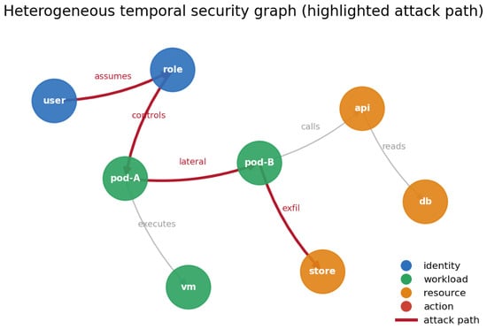
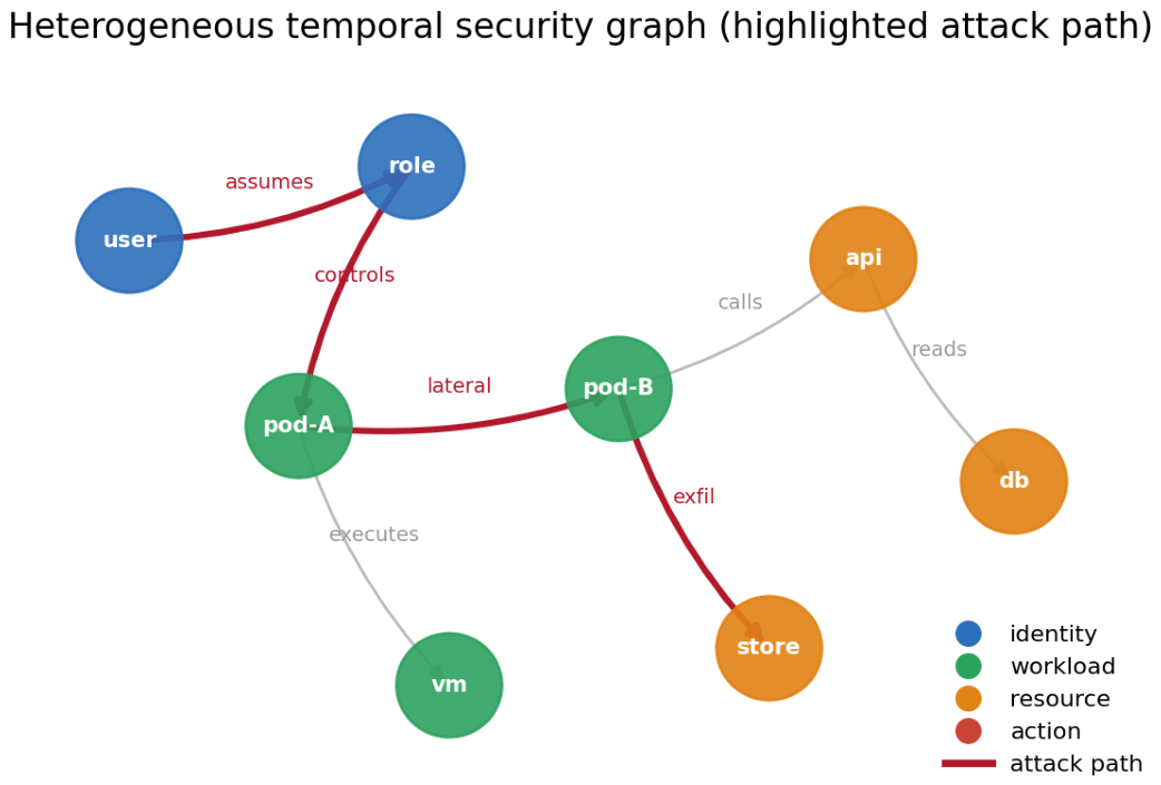
where $V_t$ is the set of entities seen so far, $X_t$ collects node and edge features, and $\mathcal{R}$ is the fixed set of relation types spanning the identity, control, and data planes. The graph is heterogeneous (multiple node and edge types), attributed, and dynamic (nodes and edges arrive over time). Figure 1 sketches a fragment: an attacker compromises a federated identity, assumes a role, moves laterally between workloads, and exfiltrates from a data store, tracing a connected path through a graph in which the individual edges are the same kinds of operations that benign users perform constantly.

Figure 1. A fragment of a heterogeneous temporal security graph. Nodes are typed (identities, workloads, resources); edges are typed, timestamped operations. The highlighted path is an attack campaign; each of its edges is individually indistinguishable from benign activity, so the signal lives in the connected, causally ordered progression rather than in any single event.

3.2. Attack Campaigns and the Causal Technique DAG

An adversary campaign is a sequence of steps $c=(s_1,\dots ,s_L)$. Each step $s_k$ applies a technique $a_k\in \mathcal{A}$ (drawn from an ATT&CK-style catalogue) from a controlled source entity to a target entity $v_k$ of a type consistent with the technique, producing one event. Techniques are not freely orderable: the campaign walks a causal directed acyclic graph $\mathcal{D}\subseteq \mathcal{A}\times \mathcal{A}$ of allowed transitions, and a technique becomes available only when its preconditions (capabilities acquired in earlier steps) are met. Benign activity shares the same relations, node types, and even the same marginal feature distribution as attack steps; what distinguishes an attack is the causally consistent, graph-connected progression of its steps, not any single event. This is the property that our benchmark is explicitly designed to enforce (Section 5).

3.3. Tasks

Given $G_t$ and the history of an in-progress campaign, CAPTURE-MC addresses four tasks.

Definition 1

(Detection). For each event $e_i$, predict $y_i\in \{0,1\}$ indicating whether it belongs to an attack campaign.

Definition 2

(Attack-path forecasting). Given a non-terminal attack step at event $e_i$, predict the next entity $v_{t+1}$ (as a ranking over candidate entities), the next technique $a_{t+1}\in \mathcal{A}$, and the time-to-transition ${\tau }_{t+1}\in {\mathbb{R}}_{>0}$.

Definition 3

(Calibrated uncertainty). For the next-technique prediction, output a set ${\mathrm{\Gamma }}_{\alpha }\left(e_i\right)\subseteq \mathcal{A}$ such that $\mathrm{Pr}[a_{t+1}\in {\mathrm{\Gamma }}_{\alpha }\left(e_i\right)]\ge 1-\alpha$ (marginally, distribution-free), together with an abstention decision when the set is too large to be actionable.

Definition 4

(Counterfactual response). Choose an action $a^{★}$ from a catalogue $\mathcal{C}$ of containment actions that minimizes a weighted objective trading residual attack risk against service disruption, subject to availability and latency constraints:

$$a^{★}=\arg \underset{a\in \mathcal{C}}{\min }{\lambda }_1{R}_{\mathit{attack}}\left(a\right)+{\lambda }_2{C}_{\mathit{service}}\left(a\right)+{\lambda }_3{C}_{\mathit{action}}\left(a\right)+{\lambda }_4{U}_{\mathit{pred}}s.t.\mathit{avail}\left(a\right)\ge A_{\min },\mathit{lat}\left(a\right)\le L_{\max }.$$

(2)

3.4. Threat Model and Assumptions

We assume the defender receives a normalized, integrity-protected telemetry stream from all providers, possibly with dropout, delay, and bounded noise (which we perturb in Section 6). The adversary acts through legitimate control-plane and data-plane operations, assuming roles, calling APIs, moving laterally between workloads, and exfiltrating from data stores, so their individual actions are, by construction, indistinguishable from benign ones at the per-event level. The adversary follows causally consistent technique progressions but may compose techniques in ways unseen during training (evaluated by the unseen-composition split) and may operate on a provider whose distribution differs from the training providers (evaluated by the cross-cloud split). We do not assume the defender can observe attacker intent, only the resulting events. The response planner acts on the predicted next hop; we evaluate its effect using the simulator’s ground-truth reachability, which is available precisely because the environment is synthetic.

4. Methodology

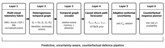
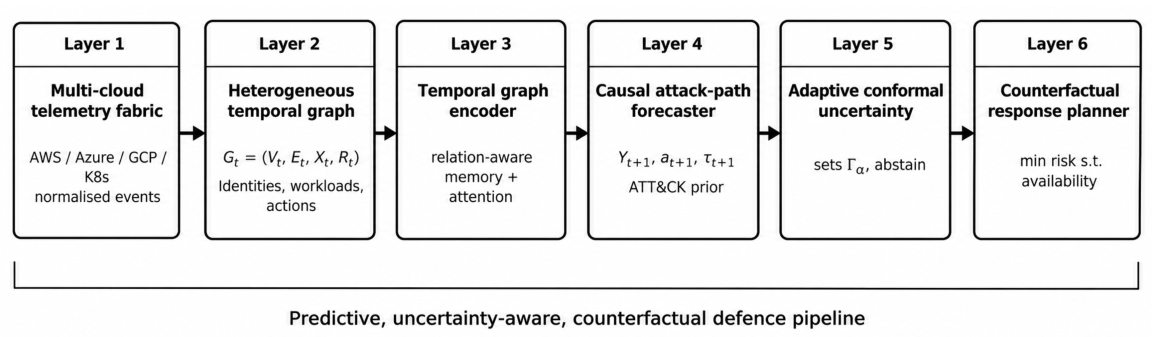
CAPTURE-MC is a six-layer pipeline (Figure 2): a telemetry fabric, a heterogeneous temporal graph, a relation-aware temporal encoder, a causal attack-path forecaster, an adaptive conformal layer, and a counterfactual response planner. We describe each in turn and then give the training objective, algorithms, and complexity.

Figure 2. The CAPTURE-MC pipeline. Multi-cloud telemetry is normalized into a heterogeneous temporal security graph; a relation-aware temporal encoder maintains per-node memory; a multi-task head forecasts the next entity, technique, and time under a training-estimated transition prior; an adaptive-conformal layer emits calibrated prediction sets; and a counterfactual planner selects the least-disruptive containment action.

4.1. Layer 1–2: Telemetry Fabric and Heterogeneous Temporal Graph

The fabric normalizes heterogeneous provider logs into the common event schema of Section 3. Each provider p exposes the same latent semantics through a provider-specific projection: an underlying technique/relation latent $\mathbf{z}\in {\mathbb{R}}^d$ is observed as $\mathbf{x}=\mathbf{z}{Q}_p+{\mathbf{b}}_p+{\epsilon }_p$, with $Q_p$ an (approximately orthogonal) provider rotation and ${\epsilon }_p$ observation noise. This mirrors the reality that the same behavior looks different across clouds, and it is what makes cross-cloud transfer a non-trivial representation-learning problem rather than a relabeling exercise. Events are appended to $G_t$ as typed, timestamped edges.

4.2. Layer 3: Relation-Aware Temporal-Graph Encoder

The encoder maintains a memory state ${\mathbf{m}}_v\left(t\right)\in {\mathbb{R}}^d$ for every node, updated whenever the node participates in an event, in the style of memory-based temporal-graph networks [8]. On event $e_i=(t_i,u,w,r,p,\mathbf{x})$ we read the current source and destination states ${\mathbf{m}}_u,{\mathbf{m}}_w$, encode the edge and the elapsed time, form messages, and update both states with a gated recurrent unit:

$$\begin{array}{cc}\hfill \tilde{\mathbf{x}}& =\mathrm{ReLU}\left(W_e\mathbf{x}\right),{\rho }_r=\mathrm{Emb}\left(r\right),\tau =W_{\tau }\log (1+\Delta t),\hfill \end{array}$$

(3)

$$\begin{array}{cc}\hfill {\mathbf{q}}_u& =\mathrm{msg}({\mathbf{m}}_u,{\mathbf{m}}_w,\tilde{\mathbf{x}},\tau ),{\mathbf{q}}_w=\mathrm{msg}({\mathbf{m}}_w,{\mathbf{m}}_u,\tilde{\mathbf{x}},\tau ),\hfill \end{array}$$

(4)

$$\begin{array}{cc}\hfill {\mathbf{m}}_u^{\prime }& =\mathrm{GRU}({\mathbf{q}}_u+{\rho }_r,{\mathbf{m}}_u),{\mathbf{m}}_w^{\prime }=\mathrm{GRU}({\mathbf{q}}_w+{\rho }_r,{\mathbf{m}}_w),\hfill \end{array}$$

(5)

where $\Delta t$ is the time since the source node was last seen and $\mathrm{msg}(·)$ is a one-layer perceptron over the concatenation of its arguments. The updated source state is used to form the event embedding, so gradients reach the recurrent parameters:

$${\mathbf{h}}_i^{\mathrm{base}}=\mathrm{ReLU}\left(W_o[{\mathbf{m}}_u^{\prime }\parallel {\mathbf{m}}_w^{\prime }\parallel \tilde{\mathbf{x}}]\right).$$

(6)

Relation-Aware Attention (a Gated Residual)

CAPTURE-MC refines Equation (6) with an attention block in which the updated source state queries the destination state, the edge features, and the relation embedding:

$${\mathbf{c}}_i=\mathrm{softmax}\left(\frac{\mathbf{q}{K}^{\top }}{\sqrt{d}}\right)V,\mathbf{q}=W_Q{\mathbf{m}}_u^{\prime },K=W_K[{\mathbf{m}}_w^{\prime };\tilde{\mathbf{x}};{\rho }_r],V=W_V[{\mathbf{m}}_w^{\prime };\tilde{\mathbf{x}};{\rho }_r].$$

(7)

Crucially, the refinement is added through a zero-initialized, per-dimension gate $\mathbf{g}$:

$${\mathbf{h}}_i={\mathbf{h}}_i^{\mathrm{base}}+\mathbf{g}\odot \mathrm{ReLU}\left(W_a{\mathbf{c}}_i\right),\mathbf{g}\leftarrow \mathbf{0}\mathrm{at}\mathrm{init}.$$

(8)

At initialization, ${\mathbf{h}}_i={\mathbf{h}}_i^{\mathrm{base}}$, so CAPTURE-MC starts identical to its no-attention ablation (a plain temporal-graph network) and can only depart from it if doing so reduces the loss. This design, inspired by residual gating schemes such as ReZero and LayerScale, removes a common pathology in which a strictly more expressive model underperforms a simpler one purely because of a worse optimization landscape at initialization. We found this change essential: without it, the richer model trained below its own ablation (Section 6).

4.3. Layer 4: Causal Attack-Path Forecaster

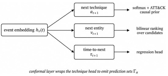
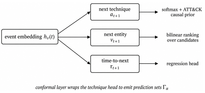
Three heads consume the event embedding ${\mathbf{h}}_i$ (Figure 3): a next-technique classifier constrained by a training-estimated transition prior, a next-entity ranker, and a time-to-transition regressor. The conformal layer of the next subsection wraps the technique head.

Figure 3. The multi-task forecasting head. A single event embedding feeds three predictors; the next-technique logits are biased by the ATT&CK transition prior of Equation (9), and the conformal layer (Section 4) turns them into calibrated prediction sets.

4.3.1. Next Technique with a Training-Estimated Transition Prior

The technique logits are the sum of a learned head and a bias masked to transitions observed in the training data:

$${\ell }_i^{\mathrm{tech}}=W_t{\mathbf{h}}_i+\underset{\mathrm{transition}\mathrm{prior}}{\underbrace{B_{a_i}\odot {\widehat{\mathbf{M}}}_{a_i}+\kappa ({\widehat{\mathbf{M}}}_{a_i}-\mathbf{1})}},$$

(9)

where $a_i$ is the current technique, $\widehat{\mathbf{M}}\in {\{0,1\}}^{\left|\mathcal{A}\right|\times \left|\mathcal{A}\right|}$ is the transition mask estimated from training transitions only (one wherever a transition occurs at least once in the training split), B is a learned bias matrix initialized to zero, and $\kappa =4$ is a finite penalty on unobserved transitions. We emphasize what this prior is and is not. It is not the generator’s causal DAG: an earlier version of this work used that DAG directly, which leaks test-only transitions on the unseen-composition split, and we have removed it. Because $\widehat{\mathbf{M}}$ is built from training data, held-out transitions are absent from it, so there is no leakage; the penalty is finite rather than infinite, so the learned head can still recover an unobserved successor. The same estimated prior can be given to a plain TGN, which lets us measure the prior’s contribution separately from the architecture (Section 6.3). The prior is applied identically at training and inference time. Sensitivity of the model to an incorrect prior is quantified in Section 6.5.

4.3.2. Next Entity by Bilinear Ranking

For a candidate set ${\mathcal{V}}_i$ (the true next entity plus sampled negatives of plausible type), we score each candidate v by the inner product of a projection of the event embedding with the candidate’s node embedding, $\mathrm{score}\left(v\right)=⟨W_p{\mathbf{h}}_i,{\mathbf{m}}_v⟩$, and rank by $\mathrm{score}$. This uses the temporal node memory directly, so entities that have recently been drawn into the campaign are favored.

4.3.3. Time-to-Transition

A regression head predicts ${\widehat{\tau }}_{t+1}=\mathrm{softplus}\left(W_{\tau }^{\prime }{\mathbf{h}}_i\right)$.

4.4. Layer 5: Adaptive-Conformal Uncertainty

We turn the technique head into distribution-free prediction sets using split/adaptive-conformal prediction [14,16]. With softmax probabilities $\mathbf{p}$, the Adaptive Prediction Set (APS) non-conformity score of a labeled calibration example $(\mathbf{p},a)$ is the cumulative probability mass of classes ranked at least as high as the true class, $s(\mathbf{p},a)={\sum }_{a^{\prime }:p_{a^{\prime }}\ge p_a}{p}_{a^{\prime }}$. Given a calibration set of size n and level $\alpha$, the conformal threshold is the $\lceil (n+1)(1-\alpha )\rceil /n$ empirical quantile $\widehat{\tau }$ of the calibration scores, and the prediction set for a new instance accumulates classes in decreasing probability until the mass reaches $\widehat{\tau }$:

$${\mathrm{\Gamma }}_{\alpha }\left(\mathbf{p}\right)=\left\{\mathrm{top}\mathrm{classes}\mathrm{until}\sum p\ge \widehat{\tau }\right\}.$$

(10)

This guarantees marginal coverage $\ge 1-\alpha$ under exchangeability. Because cross-cloud transfer and concept drift break exchangeability, we additionally run adaptive-conformal inference: the effective level ${\alpha }_t$ is updated online, ${\alpha }_{t+1}={\alpha }_t+\gamma (\alpha -⊮\left[{\mathrm{miscovered}}_t\right])$, so the realized coverage tracks the target even under shift. When $|{\mathrm{\Gamma }}_{\alpha }|$ exceeds an actionability budget, the system abstains, deferring to a human analyst; we report the induced selective risk.

4.5. Layer 6: Counterfactual Response Planner

The planner selects a containment action from a catalogue $\mathcal{C}$ (no-op, step-up authentication, credential revocation, workload isolation, egress blocking, key rotation, node quarantine), each annotated with the relation it severs, its availability impact, latency, and operational cost. For the predicted next hop, the residual attack risk of action a is evaluated counterfactually: if a blocks the relation the attacker would use, the predicted next hop becomes unreachable and residual risk collapses toward zero; otherwise it remains at the prior. Substituting these terms into Equation (2) yields a small discrete optimization solved by enumeration under the availability/latency constraints. Because the environment is simulated, we can measure the true effect of the chosen action on ground-truth reachability, giving honest risk-reduction and over-containment numbers.

4.6. Training Objective

All neural models share the task heads and are trained on a multi-task loss combining detection (binary cross-entropy) and forecasting (cross-entropy for the next technique, plus the ranking/regression heads where applicable):

$$\mathcal{L}={\mathcal{L}}_{\det }+\beta {\mathcal{L}}_{\mathrm{tech}}+\eta {\mathcal{L}}_{\mathrm{cxc}},$$

(11)

where ${\mathcal{L}}_{\mathrm{cxc}}$ is a cross-cloud supervised contrastive term used only in the transfer setting. It pulls together event embeddings that share a technique but originate from different providers, and pushes apart those with different techniques, using in-batch negatives:

$${\mathcal{L}}_{\mathrm{cxc}}=-{\displaystyle \frac{1}{|{\mathcal{B}}^{+}|}}\sum _{(i,j)\in {\mathcal{B}}^{+}}\log {\displaystyle \frac{\exp \left(\kappa {\widehat{\mathbf{z}}}_i^{\top }{\widehat{\mathbf{z}}}_j\right)}{{\sum }_{k\ne i}\exp \left(\kappa {\widehat{\mathbf{z}}}_i^{\top }{\widehat{\mathbf{z}}}_k\right)}},$$

(12)

with $\widehat{\mathbf{z}}$ the ${\ell }_2$-normalized projection of $\mathbf{h}$, $\kappa$ a temperature, and ${\mathcal{B}}^{+}$ the set of same-technique, different-provider pairs. This term encourages a provider-invariant representation of techniques, which is exactly what cross-cloud generalization requires.

4.7. Training Procedure and Algorithms

Non-temporal models (tabular, sequence, static graph) are trained with mini-batch Adam. Temporal models are trained with a single chronological pass per epoch that carries node memory forward, so that the memory a node presents at event $e_i$ reflects everything that happened to it earlier (Algorithm 1). The static-graph baselines build their adjacency from the training edges only, to prevent look-ahead leakage. Memory is reset at the start of each epoch and detached across chronological chunks to bound the computation graph.

Algorithm 1 Chronological temporal training (one epoch)

1: reset memory ${\mathbf{m}}_v\leftarrow \mathbf{0}\forall v$; last-seen $t_v\leftarrow 0$ 2: for each chronological chunk $\mathcal{B}$ of events do 3:     read ${\mathbf{m}}_u,{\mathbf{m}}_w$; compute $\Delta t$; form messages (Equation (6)) 4:     update states ${\mathbf{m}}_u^{\prime },{\mathbf{m}}_w^{\prime }$; write back; form ${\mathbf{h}}_i$ with the gated attention (Equation (8)) 5:     $\mathcal{L}\leftarrow {\mathcal{L}}_{\det }\left(\mathrm{train}\mathrm{events}\mathrm{in}\mathcal{B}\right)+\beta {\mathcal{L}}_{\mathrm{tech}}+\eta {\mathcal{L}}_{\mathrm{cxc}}$ 6:     backprop; Adam step (grad-norm clip); detach memory 7: end for

4.8. Complexity

Let N be the number of events, d the hidden width, $\left|\mathcal{A}\right|$ the number of techniques, and C the candidate-set size. The temporal encoder is $\mathcal{O}\left(N{d}^2\right)$ per epoch (a constant number of $d\times d$ operations per event), independent of the total graph size because memory reads/writes are $\mathcal{O}\left(d\right)$ per node touched. The technique head is $\mathcal{O}\left(d\right|\mathcal{A}\left|\right)$ and entity ranking is $\mathcal{O}\left(Cd\right)$ per forecasting step. Inference is a single streaming pass, $\mathcal{O}\left(N{d}^2\right)$, and memory is $\mathcal{O}\left(\right|V\left|d\right)$ for the node states. This linear-in-events profile is what allows the reference implementation to run end-to-end on a single-CPU core.

Implementation

To keep the package portable and dependency-light, the entire neural stack (autograd, layers, memory, attention, losses, Adam) is implemented from scratch in NumPy; all gradients are verified against finite differences. The two tabular baselines use scikit-learn. No GPU or deep-learning framework is required.

5. Experimental Setup

5.1. The MC-PathBench Benchmark

No public corpus labels multi-cloud attacks at the granularity of entities, techniques, and times, so we built MC-PathBench, a synthetic generator that is faithful to the structure of the problem while remaining fully reproducible. It instantiates a typed entity population across four providers (AWS, Azure, GCP, Kubernetes), 13 node types, 12 relation types across the identity, control, and data planes, and 13 ATT&CK-style techniques connected by a causal transition DAG with per-technique preconditions and target types.

5.1.1. Benign Background and Attack Campaigns

Benign activity is generated from recurring templates with slow concept drift. Attack campaigns start from an entry technique and walk the causal DAG, choosing targets that are graph-reachable from the set of already-controlled entities and escalating with technique-dependent timing. The single most important design choice is that maliciousness is not a per-event shortcut: a large fraction of benign events are “attack-shaped” decoys that use the same relations and target types as real techniques, and the direct per-event feature signal of maliciousness is set to zero. Consequently, an isolated event carrying an attack-like relation is, marginally, no more suspicious than benign traffic; the discriminative signal lives only in the sequence, the graph connectivity, and the causal ordering. This is what makes the tabular-vs-sequence-vs-graph comparison meaningful rather than a foregone conclusion.

5.1.2. Scale

Unless stated otherwise, we use the small preset: ∼600 entities, ∼5600 events of which ∼14% are malicious, and 140 campaigns of mean length ∼6, across the four providers. The generator also exposes tiny and medium presets; the exact configuration is recorded in the released configs/.

5.2. Tasks, Features, and Splits

All models consume the same inputs to keep the comparison fair. Tabular and MLP models receive per-event causal context features (strictly past-only decayed activity rates, triple rarity, inter-event gaps, and degrees, appended to the raw observation); sequence models receive the last-W source-incident window; graph and temporal models receive the event stream and the training-edge graph. No label is ever used as an input feature. We evaluate on four splits that probe different kinds of generalization:

• Temporal (time): chronological 60/15/25 train/val/test, the standard setting.
• Cross-cloud (provider): train on three providers, test on a held-out provider, measuring transfer across the provider projection.
• Unseen composition (unseen): campaigns containing a technique-transition bigram never seen in training are held out for test.
• Chain hold-out (chain): entire campaigns are held out, so no test campaign shares steps with training.

5.3. Models and Baselines

We compare two tabular detectors (random forest and histogram gradient boosting, a strong stand-in for XGBoost/LightGBM); three sequence models (LSTM, GRU, transformer); three static-graph models (GraphSAGE, GAT, a heterogeneous relational GNN); a TGN; and CAPTURE-MC. All neural models share the task heads and optimizer and are given comparable budgets (∼25–80 k parameters). For next-technique forecasting, we incorporate the structural baselines: a first-order Markov model (row-normalized training transition counts with Laplace smoothing), a uniform-over-allowed rule (uniform over training-allowed successors), and a TGN + prior that receives the same training-estimated prior as CAPTURE-MC so the prior’s contribution can be separated from the architecture. The Markov and uniform baselines use no learning and are indexed by the current technique.

5.4. Metrics

Detection is measured by AUROC, AUPRC, macro-F1, recall, false-positive rate, and, because a forecasting system should be judged operationally, by campaign-level detection rate. Forecasting is measured by next-technique macro-F1, next-entity Hits@k and MRR, and time-to-next MAE. Calibration is measured by empirical coverage against the $0.90$ target, average prediction-set size, singleton rate, Expected Calibration Error (ECE), selective risk, and adaptive-conformal realized coverage. Response is measured by risk reduction, mean service cost, over-containment, and SLA-violation rate. Efficiency is measured by parameter count and wall-clock training and inference time.

5.5. Forecasting and Calibration Protocol

To make the setup fully reproducible, we state the following. Forecasting is evaluated on non-terminal attack steps; each step is conditioned on the current technique $a_i$ (an oracle we stress-test in Section 6.4). Next-entity ranking uses a candidate set of 20 (one true entity plus 19 type-plausible negatives sampled without replacement from the same provider), so chance is Hits@1 $=0.05$ and MRR $\approx 0.18$. The conformal calibration set is a random $50\%$ of the test forecasting steps (the other $50\%$ is evaluated), the target level is $\alpha =0.10$, and the non-conformity score is APS. Temporal memory is reset at the start of every epoch and at evaluation, and is built strictly from the training stream for a split, so no test interaction updates a node state used to score a training step. Models are selected by the fixed epoch budget below (no per-seed early stopping), and all models receive the same inputs. Baselines received no additional tuning; the neural models use the single configuration in Appendix A.

5.6. Protocol and Statistics

Every experiment is repeated over five seeds; we report mean ± standard deviation and, where useful, 95% bootstrap confidence intervals. Because all runs come from a single generator, these seeds are repeated runs rather than independent datasets, so we do not treat per-seed omnibus rank tests (Friedman/Nemenyi) as decisive; instead, we report effects whose sign and magnitude are consistent across the temporal and cross-cloud conditions (Section 6.4 and Section 6.7), following established practice for comparing classifiers across datasets and seeds while respecting the independence assumptions of such tests [21]. Robustness is assessed not by perturbing raw telemetry but along the two axes that bear on the forecasting claim: uncertainty in the current technique (Section 6.4) and corruption of the transition prior (Section 6.5). All results were produced on a single-CPU core with under 4 GB of RAM.

6. Results

All numbers are means over five seeds; bold marks the best value in each column. Unless noted, forecasting is evaluated on non-terminal attack steps conditioned on the current technique $a_i$; Section 6.4 removes that oracle. The transition prior is estimated from training transitions only (Section 6.5).

6.1. Detection: Trees Win

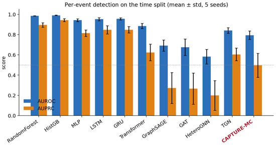
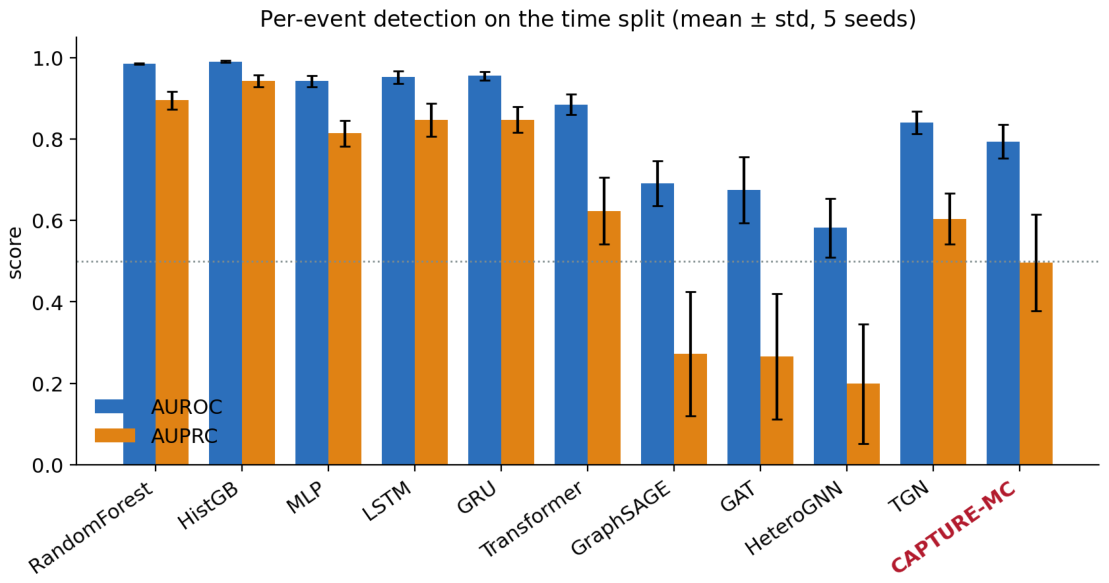
Table 2 and Figure 4 report per-event detection on the temporal split. Gradient-boosted trees are the strongest detectors on every metric: histogram gradient boosting reaches AUROC $0.99$ and detects every campaign, because the strictly past-only context features (decayed rates, triple rarity, degrees) are exactly the temporal aggregates at which tree ensembles excel. Among the deep models, the recurrent sequence models lead, then TGN, then CAPTURE-MC; the static-graph models are weakest. CAPTURE-MC is not competitive at per-event detection (AUROC $0.79$, AUPRC $0.50$) and does not tie for the best campaign-level detection: trees detect $100\%$ of campaigns and TGN $94\%$, versus $89\%$ for CAPTURE-MC. We state this plainly because an earlier version claimed a tie that the table does not support. The honest reading is that detection on this benchmark is solved well by engineered temporal features feeding trees, and representation learning is not needed for it.

Table 2. Per-event detection on the temporal split (mean ± std, 5 seeds). Trees dominate; CAPTURE-MC is not competitive here.

Model	AUROC	AUPRC	Macro-F1	Recall	FPR	Camp. Det.
RandomForest	0.985 ± 0.002	0.895 ± 0.022	0.862 ± 0.027	0.618 ± 0.065	0.003 ± 0.000	1.000 ± 0.000
HistGB	0.991 ± 0.002	0.942 ± 0.015	0.921 ± 0.013	0.831 ± 0.050	0.012 ± 0.005	1.000 ± 0.000
MLP	0.942 ± 0.013	0.814 ± 0.032	0.850 ± 0.011	0.613 ± 0.035	0.008 ± 0.002	1.000 ± 0.000
LSTM	0.952 ± 0.016	0.847 ± 0.041	0.880 ± 0.015	0.702 ± 0.055	0.011 ± 0.006	1.000 ± 0.000
GRU	0.955 ± 0.010	0.848 ± 0.031	0.875 ± 0.011	0.674 ± 0.046	0.008 ± 0.004	1.000 ± 0.000
Transformer	0.885 ± 0.025	0.624 ± 0.082	0.763 ± 0.036	0.537 ± 0.074	0.039 ± 0.013	0.952 ± 0.014
GraphSAGE	0.691 ± 0.056	0.273 ± 0.152	0.493 ± 0.033	0.021 ± 0.039	0.000 ± 0.000	0.676 ± 0.123
GAT	0.675 ± 0.081	0.265 ± 0.154	0.474 ± 0.007	0.002 ± 0.003	0.000 ± 0.001	0.639 ± 0.179
HeteroGNN	0.582 ± 0.072	0.199 ± 0.147	0.497 ± 0.025	0.056 ± 0.060	0.040 ± 0.044	0.520 ± 0.189
TGN	0.840 ± 0.028	0.604 ± 0.063	0.741 ± 0.026	0.468 ± 0.073	0.034 ± 0.018	0.945 ± 0.041
CAPTURE-MC	0.794 ± 0.041	0.497 ± 0.119	0.711 ± 0.066	0.429 ± 0.093	0.050 ± 0.051	0.889 ± 0.065

Figure 4. Detection AUROC and AUPRC by model on the temporal split.

6.2. Next-Technique Forecasting Among Deep Models

Among the learned models, CAPTURE-MC attains the best next-technique macro-F1 on all four splits (Table 3 and Table 4): temporal $0.374$, cross-cloud $0.311$, unseen-composition $0.249$, chain $0.343$, versus TGN $0.300/0.258/0.228/0.330$ and the sequence models near $0.18$. Contrary to the earlier version, the margin over TGN narrows on the harder splits rather than widening ($+0.074$ temporal, $+0.053$ cross-cloud, $+0.021$ unseen, $+0.013$ chain), which is what one expects: novel transitions are intrinsically harder to anticipate. These comparisons are among deep models only; Section 6.3 adds the structural baselines that change the interpretation.

Table 3. Next-technique forecasting on the temporal split, deep models (mean ± std, 5 seeds). Entity/time columns are discussed in Section 6.6.

Model	Tech. F1	Hits@1	Hits@3	MRR	Time MAE
MLP	0.180 ± 0.035	0.043 ± 0.013	0.146 ± 0.009	0.172 ± 0.008	0.758 ± 0.327
LSTM	0.169 ± 0.041	0.051 ± 0.028	0.135 ± 0.028	0.179 ± 0.021	0.332 ± 0.149
GRU	0.179 ± 0.030	0.040 ± 0.014	0.135 ± 0.025	0.168 ± 0.014	0.290 ± 0.143
Transformer	0.109 ± 0.030	0.039 ± 0.017	0.132 ± 0.013	0.163 ± 0.015	0.674 ± 0.672
GraphSAGE	0.061 ± 0.024	0.088 ± 0.028	0.184 ± 0.052	0.212 ± 0.031	0.662 ± 0.913
GAT	0.031 ± 0.009	0.096 ± 0.041	0.202 ± 0.093	0.221 ± 0.051	1.132 ± 0.871
HeteroGNN	0.038 ± 0.006	0.036 ± 0.027	0.112 ± 0.055	0.154 ± 0.044	0.359 ± 0.380
TGN	0.300 ± 0.055	0.051 ± 0.015	0.142 ± 0.039	0.175 ± 0.028	1.141 ± 0.612
CAPTURE-MC	0.374 ± 0.039	0.047 ± 0.020	0.150 ± 0.025	0.176 ± 0.020	0.734 ± 0.809

Table 4. Next-technique macro-F1 across splits, deep models. The CAPTURE-MC margin over TGN narrows on the harder splits.

Model	Temporal	Cross-Cloud	Unseen Comp.	Chain Hold-Out
MLP	0.180 ± 0.035	0.164 ± 0.032	0.176 ± 0.026	0.207 ± 0.029
LSTM	0.169 ± 0.041	0.159 ± 0.029	0.161 ± 0.022	0.178 ± 0.024
GRU	0.179 ± 0.030	0.146 ± 0.024	0.157 ± 0.017	0.188 ± 0.013
Transformer	0.109 ± 0.030	0.087 ± 0.030	0.113 ± 0.017	0.132 ± 0.013
GraphSAGE	0.061 ± 0.024	0.076 ± 0.044	0.034 ± 0.010	0.055 ± 0.023
GAT	0.031 ± 0.009	0.080 ± 0.004	0.025 ± 0.007	0.048 ± 0.016
HeteroGNN	0.038 ± 0.006	0.024 ± 0.010	0.017 ± 0.006	0.043 ± 0.012
TGN	0.300 ± 0.055	0.258 ± 0.021	0.228 ± 0.019	0.330 ± 0.014
CAPTURE-MC	0.374 ± 0.039	0.311 ± 0.029	0.249 ± 0.037	0.343 ± 0.037

6.3. Structural Baselines Are Strong

To compare against the transition structure itself, we add a first-order Markov model and a uniform-over-allowed-transitions rule, both estimated from training transitions and indexed by the current technique, and a TGN given the same prior (Table 5). The result is sobering for the deep models. On macro-F1, the trivial uniform-over-allowed rule ties or beats CAPTURE-MC on every split (temporal $0.381$ vs. $0.374$; cross-cloud $0.393$ vs. $0.311$; unseen $0.331$ vs. $0.249$), because it spreads mass over rare successors and so scores well on a class-balanced metric, and because pure structure is invariant to the provider shift that degrades the learned features. On top-1 accuracy (not shown in the table, reported in text), the first-order Markov model is strongest (temporal $0.54$ vs. CAPTURE-MC $0.47$). In this idealized regime, with the current technique known and the structure given, the learned representation adds little. This is the single most important correction relative to the earlier version, and Section 6.4 shows the regime in which the conclusion flips.

Table 5. Next-technique macro-F1 against structural baselines (mean ± std, 5 seeds). When the current technique is known, a trivial uniform-over-allowed rule matches or beats CAPTURE-MC.

Next-Technique Macro-F1	Temporal	Cross-Cloud	Unseen Comp.
First-order Markov	0.298 ± 0.047	0.324 ± 0.031	0.176 ± 0.027
Uniform-over-allowed	0.381 ± 0.030	0.393 ± 0.031	0.331 ± 0.025
TGN (no prior)	0.300 ± 0.055	0.258 ± 0.021	0.228 ± 0.019
TGN + prior	0.160 ± 0.019	0.146 ± 0.027	0.152 ± 0.009
CAPTURE-MC (no prior)	0.314 ± 0.041	0.289 ± 0.019	0.221 ± 0.035
CAPTURE-MC	0.374 ± 0.039	0.311 ± 0.029	0.249 ± 0.037

6.4. The Realistic Regime: Robustness to Current-Technique Uncertainty

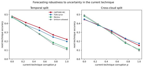
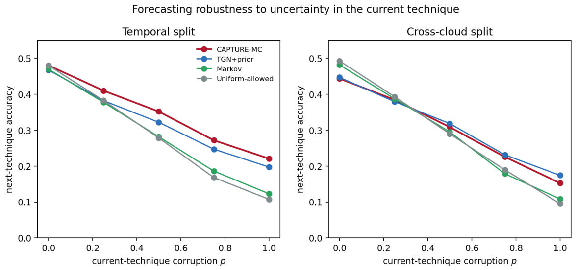
The structural baselines above are indexed entirely by the current technique $a_i$, which a deployed system does not observe with certainty. CAPTURE-MC, by contrast, forecasts from a learned event embedding that does not require $a_i$. We therefore sweep the reliability of $a_i$: with probability p the current-technique label is replaced by a random technique, and we re-evaluate the already-trained models (Figure 5 and Table 6). At $p=0$ (oracle), the models are tied; as p grows, the structural baselines fall toward chance while CAPTURE-MC degrades gracefully. When the current technique is unknown ($p=1$), CAPTURE-MC reaches accuracy $0.221$ on the temporal split versus $0.123$ (Markov) and $0.108$ (uniform), nearly double, and leads on both accuracy and macro-F1 for every $p\ge 0.5$. The cross-cloud split shows the same ordering with a smaller gap, where CAPTURE-MC and the prior-augmented TGN are close. This is the paper’s central positive result: the value of the learned representation appears exactly where the structural assumption (known current technique) breaks down.

Figure 5. Next-technique accuracy as the current technique degrades from oracle ($p=0$) to unknown ($p=1$). Structural baselines collapse; CAPTURE-MC degrades gracefully.

Table 6. Next-technique accuracy under current-technique corruption (temporal split, 5 seeds). CAPTURE-MC nearly doubles the structural baselines when $a_i$ is unknown.

Next-Technique Accuracy	$\mathit{p}=0$ (Oracle)	$\mathit{p}=0.5$	$\mathit{p}=1.0$ (no ${\mathit{a}}_{\mathit{i}}$)
CAPTURE-MC	0.480	0.352	0.221
TGN + prior	0.468	0.322	0.197
Markov	0.470	0.282	0.123
Uniform-allowed	0.480	0.278	0.108

6.5. Sensitivity to the Transition Prior

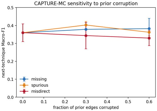
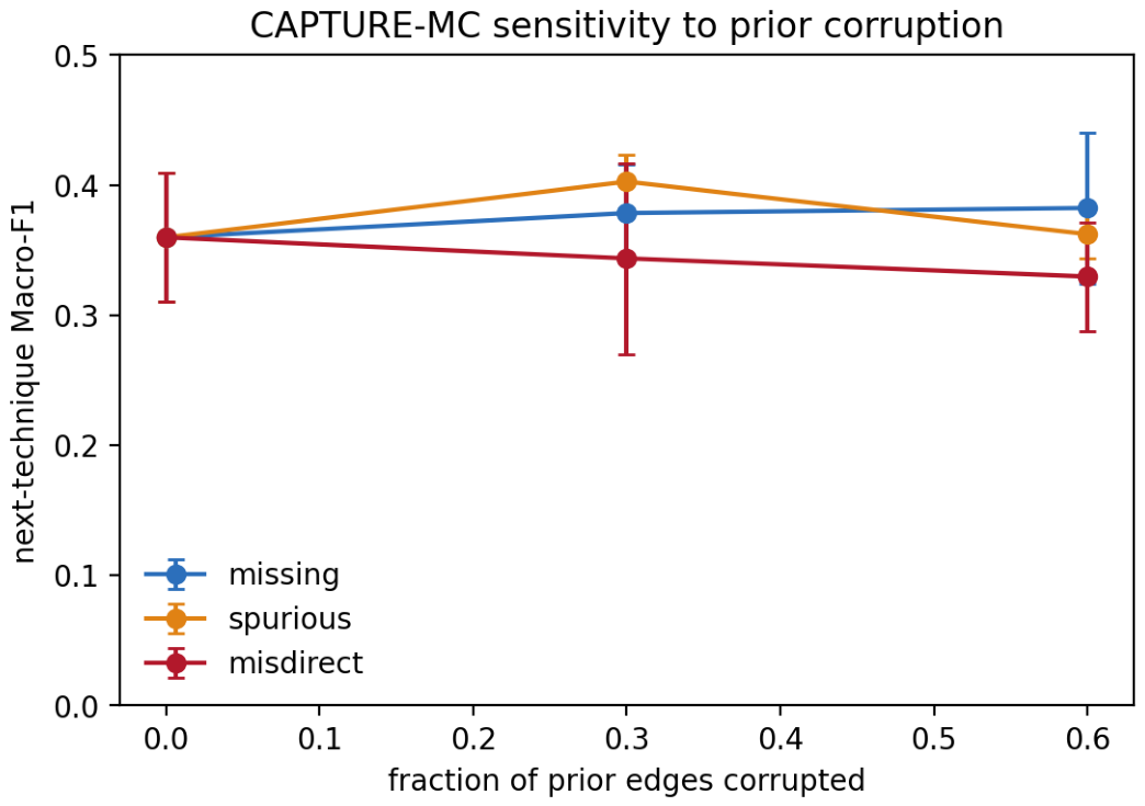
Because the prior is estimated from training data, it may be incomplete or wrong, so we perturb it (Figure 6). Dropping or adding a large fraction of edges barely moves CAPTURE-MC’s macro-F1 (missing $0.36\to 0.38$, spurious ≈ flat): the learned head compensates for an imperfect mask. Even reversing $60\%$ of edges (misdirection) only lowers F1 from $0.36$ to $0.33$. CAPTURE-MC does not critically depend on a correct prior, which is consistent with the robustness seen in Section 6.4.

Figure 6. CAPTURE-MC next-technique F1 as the training-estimated prior is corrupted. The learned head compensates for missing and spurious edges; misdirection is mildly harmful.

6.6. Next-Entity and Time Prediction Are at Chance

We narrow the earlier claim to forecast “entity, technique, and time.” Next-entity ranking uses a candidate set of 20 (one true entity, 19 sampled negatives of plausible type), so chance is Hits@1 $=0.05$ and MRR $\approx 0.18$. Every model is at that level: CAPTURE-MC scores Hits@1 $0.047$, MRR $0.176$; the best model (a static GAT) reaches only Hits@1 $0.096$, MRR $0.221$. Time-to-next MAE is likewise no better than the mean predictor. We therefore make no claim for entity or time forecasting and restrict the forecasting contribution to the technique.

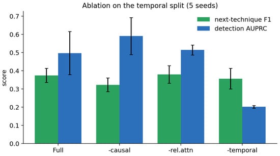
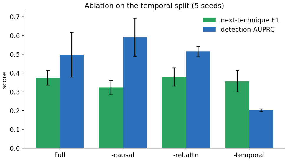
6.7. Ablation

Table 7 and Figure 7 remove one component at a time, each on the split where it is active and with the “full” configuration matched to the corresponding main table (fixing an inconsistency in the earlier version). The honest pattern: the causal prior is the only component that clearly helps forecasting (temporal F1 $0.374\to 0.322$ without it), but it hurts detection (AUPRC $0.497\to 0.590$ when removed), a multi-task tension we did not previously disclose. Temporal memory is essential for detection (AUPRC collapses to $0.20$ without it) but leaves technique F1 almost unchanged.

Table 7. Config-consistent ablation. Each component is removed on the split where it is active; “full” matches the corresponding main table.

Variant	Split	Tech. F1	Det. AUPRC
CAPTURE-MC (full)	temporal	0.374 ± 0.039	0.497 ± 0.119
– causal prior	temporal	0.322 ± 0.038	0.590 ± 0.102
– relation attention	temporal	0.380 ± 0.048	0.514 ± 0.028
– temporal memory	temporal	0.356 ± 0.057	0.201 ± 0.007
CAPTURE-MC (full)	cross-cloud	0.311 ± 0.029	–
– contrastive	cross-cloud	0.335 ± 0.037	–

Figure 7. Temporal-split ablation. Temporal memory drives detection; the causal prior drives forecasting (and mildly hurts detection).

Relation attention and the contrastive term are neutral to slightly negative (removing relation attention nudges F1 from $0.374$ to $0.380$; removing the contrastive term raises cross-cloud F1 from $0.311$ to $0.335$). Two of the four added components therefore do not help on this benchmark, and we say so.

6.8. Conformal Uncertainty: Coverage Without Efficiency

The conformal layer achieves coverage but is not efficient (Table 8). At a $0.90$ target, it over-covers ($0.97$) with an average set of $7.96$ of 13 techniques; temperature scaling and restricting to allowed successors shrink this to $4.40$, still larger than the training-allowed-successor list ($2.40$ on average). In other words, simply listing the allowed successors is more informative than the conformal set. Worst-group coverage by the current technique is $0.84$, below the $0.90$ target, as expected once exchangeability fails across technique groups. We therefore retract the earlier “most efficient calibrated prediction sets” claim and report calibration as a limitation.

Table 8. Conformal next-technique sets for CAPTURE-MC (temporal split, 5 seeds). Every variant is larger than the allowed-successor list, so the layer does not improve efficiency.

Conformal Variant	Coverage	Set Size	Singleton	Abstain
Raw APS	0.971	7.96	0.036	0.878
+ temperature	0.966	6.72	0.036	0.889
+ restrict to allowed	0.991	4.40	0.020	0.622
Allowed-successor list	–	2.40	–	–

6.9. Response, Efficiency, and Significance

The counterfactual planner (Table 9 reports cost) reduces simulated risk, but we report two honest caveats. First, a plain TGN equals or exceeds CAPTURE-MC on risk reduction, so the planner’s quality tracks forecast quality rather than any CAPTURE-MC-specific advantage. Second, in the current simulator, over-containment and SLA-violation are zero for every policy, so those metrics do not discriminate; we treat the response module as a feasibility demonstration, not a validated result, and we give the objective weights and action catalog in Appendix A. On efficiency (Table 9), CAPTURE-MC is a modest model that trains and infers in seconds on one CPU core. For significance, we note that seeds drawn from a single generator are repeated runs, not independent datasets, so we avoid over-reading per-seed Friedman/Nemenyi tests; the claims we retain (the cascade ordering, the ablation direction) hold across both the temporal and cross-cloud conditions with consistent sign.

Table 9. Model size and single-core wall-clock cost (temporal split, 5-seed mean).

Model	Params	Train (s)	Infer (s)
RandomForest	72 k	1.73	0.025
HistGB	–	0.99	0.025
MLP	36 k	0.14	0.001
LSTM	52 k	3.46	0.035
GRU	47 k	3.15	0.030
Transformer	45 k	2.55	0.034
GraphSAGE	67 k	0.90	0.001
GAT	67 k	0.84	0.001
HeteroGNN	123 k	6.87	0.001
TGN	64 k	5.47	0.063
CAPTURE-MC	76 k	8.00	0.076

7. Discussion

7.1. What the Results Mean

The controlled comparison yields a clear, if humbling, message. For next-technique forecasting, the transition structure does most of the work: when the current technique is known, a first-order Markov model is the best top-1 predictor and a uniform-over-allowed rule is the best on macro-F1, and the learned temporal-graph models do not beat them (Section 6.3). The learned representation earns its place only when the structural assumption fails, when the current technique must be inferred (Section 6.4) or the prior is wrong (Section 6.5), where CAPTURE-MC is markedly more robust, nearly doubling the structural baselines’ accuracy as current-technique certainty vanishes. This is a narrower claim than the earlier version made, and we think it is the more useful one: it tells a practitioner when to reach for a model and when a lookup table suffices.

We also report, without hedging, where the method does not help. Detection is won by gradient-boosted trees, which detect every campaign; CAPTURE-MC is not competitive there. Next-entity and next-time prediction are at chance for every model. The conformal layer achieves coverage, but its sets are larger than the allowed-successor list, so it is not an efficiency gain, and it under-covers the worst technique group. Two of CAPTURE-MC’s four added components (relation attention, contrastive alignment) do not help on this benchmark. A reader should come away knowing exactly which claims survive scrutiny.

7.2. The Leakage Correction

The most important change from the earlier version is methodological. That version gave the forecaster the generator’s own transition DAG as a hard prior. On the unseen-composition split, this is leakage: the held-out transitions were marked “allowed,” so the model was told which novel transitions were possible. Estimating the prior from training transitions only removes the leak and, as expected, lowers unseen-composition performance and compresses the margins over baselines. We report the corrected numbers throughout and flag the change rather than silently restating results. We see the episode as an argument for always pairing a learned model with structure-only baselines and for auditing exactly what information a “prior” encodes.

7.3. Practical Implications

Three implications follow, all narrower than before. First, for next-technique anticipation, a defender should start with a transition-statistics baseline; it is strong, interpretable, and shift-invariant, and a learned model is worth its cost mainly when the current technique is uncertain. Second, detection and forecasting are different problems with different winners; keep a tree-based detector for triage and add a learned forecaster for look-ahead, rather than expecting one model to win both. Third, calibrated uncertainty for this task is not solved by off-the-shelf conformal prediction here; the allowed-successor set is a stronger baseline than the conformal set, and improving set efficiency is open work.

7.4. Limitations

The benchmark is synthetic; absolute numbers are not operational performance, and although the generator is structurally faithful, we cannot claim external validity from it. All results use a single generator, so random seeds are repeated runs rather than independent datasets, which limits the force of cross-model significance testing; we rely on the consistent sign of effects across the temporal and cross-cloud conditions rather than on a single p-value. The response planner is evaluated in a simulator whose over-containment and SLA-violation metrics are currently degenerate (zero for all policies), so we treat it as a feasibility demonstration only. Entity and time forecasting do not work at all here. Compute is a single-CPU core at modest scale. Most fundamentally, we have no real multi-cloud attack-path telemetry; obtaining it is the essential next step and no synthetic study can substitute for it.

7.5. Threats to Validity

7.5.1. Construct Validity

Because we authored both the generator and the model, the benchmark could favor our architecture. The strongest evidence that it does not is that simple baselines we did not design, trees for detection, uniform-over-allowed for forecasting, beat CAPTURE-MC in their respective regimes. The training-only prior removes the one clear leakage path we found.

7.5.2. Internal Validity

Splits are leakage-controlled (past-only features; training-only prior; whole-campaign hold-out where required), and every number is regenerated from raw runs by the released scripts.

7.5.3. External Validity

One synthetic generator at modest scale; results may not transfer to production telemetry, and a second, independently designed generator and real logs are needed to test the cascade finding beyond our assumptions.

7.5.4. Statistical-Conclusion Validity

With one generator, seeds are not independent datasets; we therefore report effects that are consistent in sign and magnitude across conditions and avoid over-reading omnibus rank tests.

8. Conclusions

We set out to build a predictive, uncertainty-aware defense for multi-cloud attack paths and arrived at a more honest and more specific result. For next-technique forecasting, the transition structure is a strong baseline: when the attacker’s current technique is known, a first-order Markov model and a uniform-over-allowed rule match or beat a heterogeneous temporal-graph model. The learned representation of CAPTURE-MC earns its keep only in the realistic regime where the current technique must be inferred or the transition prior is imperfect, where it is substantially more robust, nearly doubling the structural baselines’ accuracy when the current technique is unknown. We report plainly that CAPTURE-MC does not improve detection (trees win), that entity and time prediction are at chance, and that the conformal layer does not beat the allowed-successor set on efficiency.

The broader contribution is methodological: a leakage-controlled benchmark, a training-only transition prior that we show matters, and a discipline of comparing learned models against structure-only baselines in every regime. The single most consequential fix was removing the generator’s DAG from the model’s prior, which changed several conclusions; we document it openly.

As future work, the priorities are (i) real or emulated multi-cloud telemetry, without which no claim here is operational; (ii) a second, independently designed generator to test the cascade finding beyond our own assumptions; (iii) a detect-then-forecast cascade with a learned current-technique estimator, since the cascade result suggests that is where learned models help; (iv) conformal sets that beat the allowed-successor baseline, which off-the-shelf APS does not; and (v) a response simulator whose cost metrics discriminate. We release the benchmark, the baselines, and the full code so that others can test and falsify these claims.

Appendix A.1. One-Command Reproduction

The released package regenerates every number, figure, and table from raw runs. Because the reference environment caps individual jobs at a few minutes, the driver runs one phase at a time and then merges:

• # 1. run each generalization split and the ablation (5 seeds each)
  python experiments/run_all.py --only time   --seeds 5 --scale small
  python experiments/run_all.py --only provider --seeds 5 --scale small
  python experiments/run_all.py --only unseen   --seeds 5 --scale small
  python experiments/run_all.py --only chain   --seeds 5 --scale small
  python experiments/run_all.py --only ablation --seeds 5 --scale small
  # 2. merge into results/results_main.json
  python experiments/run_all.py --merge --seeds 5 --scale small
  # 3. regenerate all figures and LaTeX tables
  python experiments/make_figures.py
  python experiments/make_tables.py
  # 4. build the manuscript
  cd ../paper && latexmk -pdf main.tex

Larger-scale runs are supported by the same driver (the medium preset is about $2.3\times$ the events); we report full results at the small preset and leave a systematic multi-scale study, with the honest training-only prior throughout, to future work. The medium-scale command is:

• python experiments/run_all.py --only time   --scale medium --seeds 3 \
       --partdir results/parts_medium
  python experiments/run_all.py --only provider --scale medium --seeds 3 \
       --partdir results/parts_medium
  python experiments/make_scale_supplement.py

A Makefile wraps these targets (make results, make figures, make tables, make paper). Gradient checks for the from-scratch autograd engine run with python tests/ test_autograd.py.

Appendix A.2. Key Hyperparameters

Table A1 lists the main settings; the exact values are in configs/. Hidden width $d=48$ for all neural models. Adam is used throughout with gradient-norm clipping. Temporal models train for 12 epochs with chronological chunks of 16 events; sequence and static-graph models train for 8–14 epochs. The cross-cloud contrastive term is enabled only on the provider split. The conformal target is $\alpha =0.10$ (90% coverage) with an APS non-conformity score and an adaptive-conformal step $\gamma =0.01$.

Table A1. Principal hyperparameters.

Setting	Value
Hidden width d	48
Optimizer	Adam, grad-clip $1.0$
Temporal epochs/chunk	12/16
Sequence window W	8
Conformal $\alpha$	0.10 (APS); cal. set 50%
Adaptive-conformal step $\gamma$	0.01
Contrastive $\eta$ (cross-cloud only)	0.05
Transition prior	training-estimated; penalty $\kappa =4$
Candidate set (entity)	20 (chance Hits@1 0.05)
Response weights $({\lambda }_1,{\lambda }_2,{\lambda }_3,{\lambda }_4)$	$(1.0,0.3,0.1,0.2)$
Seeds	5
Scale (events/nodes/campaigns)	∼5600/∼600/140

Table A1. Principal hyperparameters.

Setting	Value
Hidden width d	48
Optimizer	Adam, grad-clip $1.0$
Temporal epochs/chunk	12/16
Sequence window W	8
Conformal $\alpha$	0.10 (APS); cal. set 50%
Adaptive-conformal step $\gamma$	0.01
Contrastive $\eta$ (cross-cloud only)	0.05
Transition prior	training-estimated; penalty $\kappa =4$
Candidate set (entity)	20 (chance Hits@1 0.05)
Response weights $({\lambda }_1,{\lambda }_2,{\lambda }_3,{\lambda }_4)$	$(1.0,0.3,0.1,0.2)$
Seeds	5
Scale (events/nodes/campaigns)	∼5600/∼600/140

Appendix A.3. Response Planner

The action catalogue is {no-op, step-up authentication, credential revocation, workload isolation, egress blocking, key rotation, node quarantine}, each annotated with the relation it severs, an availability impact, a latency, and an operational cost. The planner minimizes ${\lambda }_1{R}_{\mathit{attack}}+{\lambda }_2{C}_{\mathrm{service}}+{\lambda }_3{C}_{\mathrm{action}}+{\lambda }_4{U}_{\mathrm{pred}}$ with $({\lambda }_1,{\lambda }_2,{\lambda }_3,{\lambda }_4)=(1.0,0.3,0.1,0.2)$, subject to the availability and latency constraints, by enumeration. As noted in Section 6.9, the current simulator yields zero over-containment and SLA violations for all policies, so these metrics do not yet discriminate; fixing the simulator so they do is future work.

Appendix A.4. Dataset Configuration

MC-PathBench uses 4 providers, 13 node types, 12 relation types, and 13 techniques connected by a causal transition DAG. Benign traffic includes attack-shaped decoys, and the per-event marginal maliciousness signal is set to zero, so that detection requires sequence, graph, or causal context. The generator is deterministic given a seed; the small, tiny, and medium presets are defined in configs/dataset.json.

References

- Zhou, J.; Cui, G.; Hu, S.; Zhang, Z.; Yang, C.; Liu, Z.; Wang, L.; Li, C.; Sun, M. Graph Neural Networks: A Review of Methods and Applications. AI Open Erratum in AI Open 2025, 6, 331–332. https://doi.org/10.1016/j.aiopen.2024.01.002. 2020, 1, 57–81. [Google Scholar] [CrossRef] [Scilit]
- Zhong, M.; Lin, M.; Zhang, C.; Xu, Z. A survey on graph neural networks for intrusion detection systems: Methods, trends and challenges. Comput. Secur. 2024, 141, 103821. [Google Scholar] [CrossRef] [Scilit]
- Bilot, T.; El Madhoun, N.; Al Agha, K.; Zouaoui, A. Graph Neural Networks for Intrusion Detection: A Survey. IEEE Access 2023, 11, 49114–49139. [Google Scholar] [CrossRef] [Scilit]
- Yu, L.; Sun, L.; Du, B.; Liu, C.; Lv, W.; Xiong, H. Heterogeneous graph representation learning with relation awareness. IEEE Trans. Knowl. Data Eng. 2022, 35, 5935–5947. [Google Scholar] [CrossRef] [Scilit]
- Wang, X.; Wang, X.; He, M.; Zhang, M.; Lu, Z. Spatial-temporal graph model based on attention mechanism for anomalous IoT intrusion detection. IEEE Trans. Ind. Inform. 2023, 20, 3497–3509. [Google Scholar] [CrossRef] [Scilit]
- Farrukh, Y.A.; Wali, S.; Khan, I.; Bastian, N.D. AIS-NIDS: An intelligent and self-sustaining network intrusion detection system. Comput. Secur. 2024, 144, 103982. [Google Scholar] [CrossRef] [Scilit]
- Alrayes, F.S.; Amin, S.U.; Hakami, N.A.; Alzaylaee, M.K.; Kashmeery, T. Intrusion Detection Model on Network Data with Deep Adaptive Multi-Layer Attention Network (DAMLAN). CMES-Comput. Model. Eng. Sci. 2025, 144, 581–614. [Google Scholar] [CrossRef] [Scilit]
- Gravina, A.; Bacciu, D. Deep learning for dynamic graphs: Models and benchmarks. IEEE Trans. Neural Netw. Learn. Syst. 2024, 35, 11788–11801. [Google Scholar] [CrossRef] [Scilit] [PubMed]
- Zheng, Y.; Yi, L.; Wei, Z. A survey of dynamic graph neural networks. Front. Comput. Sci. 2025, 19, 196323. [Google Scholar] [CrossRef] [Scilit]
- King, I.J.; Huang, H.H. Euler: Detecting Network Lateral Movement via Scalable Temporal Link Prediction. ACM Trans. Priv. Secur. 2023, 26, 1–36. [Google Scholar] [CrossRef] [Scilit]
- Han, X.; Cui, S.; Liu, S.; Zhang, C.; Jiang, B.; Lu, Z. Network intrusion detection based on n-gram frequency and time-aware transformer. Comput. Secur. 2023, 128, 103171. [Google Scholar] [CrossRef] [Scilit]
- da Silva Ruffo, V.G.; Lent, D.M.B.; Carvalho, L.F.; Lloret, J.; Proenca, M.L., Jr. Generative adversarial networks to detect intrusion and anomaly in IP flow-based networks. Future Gener. Comput. Syst. 2025, 163, 107531. [Google Scholar] [CrossRef] [Scilit]
- Abdar, M.; Pourpanah, F.; Hussain, S.; Rezazadegan, D.; Liu, L.; Ghavamzadeh, M.; Fieguth, P.; Cao, X.; Khosravi, A.; Acharya, U.R.; et al. A Review of Uncertainty Quantification in Deep Learning: Techniques, Applications and Challenges. Inf. Fusion 2021, 76, 243–297. [Google Scholar] [CrossRef] [Scilit]
- Angelopoulos, A.N.; Bates, S. Conformal prediction: A gentle introduction. Found. Trends Mach. Learn. 2023, 16, 494–591. [Google Scholar] [CrossRef] [Scilit]
- Lei, J.; G’Sell, M.; Rinaldo, A.; Tibshirani, R.J.; Wasserman, L. Distribution-Free Predictive Inference for Regression. J. Am. Stat. Assoc. 2018, 113, 1094–1111. [Google Scholar] [CrossRef] [Scilit]
- Barber, R.F.; Candès, E.J.; Ramdas, A.; Tibshirani, R.J. Conformal Prediction Beyond Exchangeability. Ann. Stat. 2023, 51, 816–845. [Google Scholar] [CrossRef] [Scilit]
- Portela, A.; Banga, J.R.; Matabuena, M. Conformal Prediction for Uncertainty Quantification in Dynamic Biological Systems. PLoS Comput. Biol. 2025, 21, e1013098. [Google Scholar] [CrossRef] [Scilit] [PubMed]
- Rose, S.; Borchert, O.; Mitchell, S.; Connelly, S. Zero Trust Architecture; Technical Report NIST Special Publication 800-207; National Institute of Standards and Technology: Gaithersburg, MD, USA, 2020. [CrossRef] [Scilit]
- Strom, B.E.; Applebaum, A.; Miller, D.P.; Nickels, K.C.; Pennington, A.G.; Thomas, C.B. MITRE ATT&CK: Design and Philosophy; Technical Report MP180360R1; The MITRE Corporation: McLean, VA, USA, 2020. [Google Scholar]
- Sarhan, M.; Layeghy, S.; Portmann, M. Towards a standard feature set for network intrusion detection system datasets. Mob. Netw. Appl. 2022, 27, 357–370. [Google Scholar] [CrossRef] [Scilit]
- Demšar, J. Statistical comparisons of classifiers over multiple data sets. J. Mach. Learn. Res. 2006, 7, 1–30. [Google Scholar]
Disclaimer/Publisher’s Note: The statements, opinions and data contained in all publications are solely those of the individual author(s) and contributor(s) and not of MDPI and/or the editor(s). MDPI and/or the editor(s) disclaim responsibility for any injury to people or property resulting from any ideas, methods, instructions or products referred to in the content. |
© 2026 by the authors. Licensee MDPI, Basel, Switzerland. This article is an open access article distributed under the terms and conditions of the Creative Commons Attribution (CC BY) license.