JPS-TEB Fusion Path Planning Based on COLREGs

Abstract

To address the lack of compliance with the International Regulations for Preventing Collisions at Sea (COLREGs) in conventional timed elastic band (TEB)—based dynamic path planning for autonomous surface vessels (ASVs), this study proposes an intelligent path-planning framework that integrates an improved jump point search (JPS) algorithm with a COLREGs-aware TEB approach. At the global planning layer, an enhanced JPS algorithm incorporating redundant-node elimination and cubic Bezier curve smoothing is developed to construct the JPS–PB method, thereby reducing path redundancy and improving trajectory continuity. At the local planning layer, COLREGs encounter rules are reformulated as differentiable cost functions and embedded into the TEB optimization framework, enabling rule-compliant collision avoidance in typical maritime encounter scenarios, including head-on, crossing, and overtaking situations. Simulation results demonstrate that, compared with the conventional JPS algorithm, the proposed JPS-PB method reduces the path length by up to 8.6%, decreases the cumulative steering angle by 58.6%, and lowers the maximum steering angle by 88.6% on a 12 × 12 grid environment. Furthermore, compared with the conventional TEB algorithm, the proposed COLREGs–aware TEB (CTEB) increases the Distance at the Closest Point of Approach (DCPA) by 543%, 20.5%, 4.8%, and 13.8% in starboard-crossing encounters, head-on, overtaking, and special port-side-crossing encounter scenarios, respectively. Parameter sensitivity analyses further indicate that CTEB maintains stable collision-avoidance performance and rule-compliance capability under variations in the danger–distance threshold, danger–time threshold, and COLREGs cost weight. The results verify that the proposed JPS–PB+CTEB hybrid framework effectively improves path quality, dynamic obstacle-avoidance safety, and navigation-rule compliance for autonomous ASV operations.

1. Introduction

With the rapid development of marine resource exploitation, maritime inspection, environmental monitoring, and intelligent shipping technologies, ASVs have become an important component of modern marine intelligent systems owing to their high autonomy, low operational cost, and strong environmental adaptability. As a fundamental technology for autonomous navigation, path planning plays a critical role in determining the navigation efficiency, mission performance, and operational safety of ASVs. In general, autonomous path planning can be divided into two hierarchical levels: global path planning and local path planning. The former generates a reference route from the start position to the target destination based on prior environmental information, whereas the latter performs online trajectory adjustment according to real-time perception data to avoid dynamic obstacles and potential collision risks. Recent advances in autonomous maritime navigation have driven path-planning research from conventional static planning toward integrated global–local planning, rule–constrained planning, and learning-enhanced planning strategies [1,2].

In the field of global path planning, graph-search and sampling-based algorithms, such as A*, Dijkstra, Rapidly Exploring Random Tree (RRT), and JPS, have been widely applied in known map environments. Among them, JPS is an efficient grid-based path-search algorithm developed from the conventional A* framework. By employing jump-point expansion and pruning mechanisms, JPS significantly reduces redundant node exploration and improves search efficiency [3]. However, the paths generated by the conventional JPS algorithm are typically composed of discrete polyline segments, resulting in excessive turning points, abrupt heading changes, and discontinuous curvature. Such characteristics make the generated paths unsuitable for platforms with motion inertia and maneuverability constraints, such as ASVs.

To address the limitations of JPS in complex environments, including excessive node expansion, numerous turning points, and degraded search efficiency, An et al. [4] proposed an improved bidirectional JPS algorithm. By redesigning the heuristic functions in both forward and backward search processes, the proposed method reduces the number of expanded nodes and search time. In addition, a node-optimization strategy is introduced to eliminate unnecessary nodes, followed by second-order Bezier curve smoothing to improve path continuity and trackability. Wang et al. [5] developed an improved A* algorithm by integrating the Octile heuristic function, environment-constrained adaptive weighting, and a bidirectional JPS strategy. Furthermore, a two–stage path–smoothing process was employed to reduce redundant turning points and improve path-planning efficiency in complex grid environments. Liu et al. [6] further investigated the application of bidirectional dynamic JPS for global path planning and demonstrated that improved search strategies and dynamic constraint mechanisms can effectively reduce invalid node expansion and accelerate path generation in complex environments.

Beyond standalone global planning algorithms, several studies have explored the integration of global planning and local obstacle avoidance. Yin et al. [7] combined an improved RRT* algorithm with the TEB method, where the enhanced RRT* algorithm generated a global path, and TEB performed local trajectory optimization, thereby improving path feasibility in dynamic environments. Shi et al. [8] proposed a global–local hybrid path-planning framework that combines global search results with local obstacle-avoidance mechanisms to enhance both real–time performance and navigation safety in complex environments. Although these studies provide valuable insights into JPS optimization, path pruning, and path-smoothing techniques in grid-based environments, additional efforts are still required for ASV applications, where path length, steering smoothness, and the trackability of subsequent local trajectories must be jointly considered.

For local path planning, the TEB algorithm represents a trajectory as a sequence of discrete poses associated with temporal intervals and optimizes the trajectory within a hyper-graph framework by simultaneously considering kinematic constraints, velocity constraints, acceleration constraints, and obstacle constraints [9]. Rösmann et al. [9] formulated local trajectory planning as a graph-optimization problem and achieved online trajectory generation by jointly optimizing the pose sequence and temporal intervals while satisfying vehicle motion constraints. To address trajectory oscillation and convergence issues caused by local constraints in complex environments, Chen et al. [10] incorporated fuzzy logic control into the TEB framework and improved trajectory smoothness and traversability for car-like robots operating in narrow or cluttered environments. Kulathunga et al. [11] proposed a robust TEB–based planner for collision-free navigation in unknown environments, enhancing replanning capability under environmental disturbances and unknown obstacles, thereby improving the stability of local path planning.

Despite these improvements, the obstacle-avoidance cost functions employed in conventional TEB algorithms are primarily constructed based on geometric distance, velocity, and kinematic constraints, without explicitly considering the International Regulations for Preventing Collisions at Sea (COLREGs). Consequently, when directly applied to ASV collision avoidance, conventional TEB may generate trajectories that satisfy geometric safety requirements but violate maritime navigation rules in terms of avoidance direction or passing behavior.

Unlike ground mobile robots, ASVs operating in maritime environments must not only avoid static and dynamic obstacles but also comply with COLREGs’s requirements governing head-on, crossing, and overtaking encounters. In recent years, increasing attention has been devoted to integrating COLREGs into local path-planning and collision-avoidance algorithms for autonomous vessels and ASVs. Xu et al. [12] proposed a hybrid path-planning framework that combines bidirectional A* and an improved dynamic window approach (DWA), where COLREGs constraints and ASV maneuverability characteristics are incorporated into the local evaluation function to improve rule compliance during dynamic obstacle avoidance. Liu et al. [13] introduced COLREGs constraints into an improved DWA framework, enabling local velocity sampling and trajectory evaluation to simultaneously consider collision-avoidance safety and maritime regulations. Li et al. [14] proposed a hybrid path–planning strategy integrating an improved particle swarm optimization (PSO) algorithm with DWA, achieving enhanced planning performance through cooperation between global optimization and local dynamic-window search. Similarly, Liu et al. [15] combined an improved A* algorithm with DWA to achieve integrated global path planning and local collision avoidance for ASVs.

Beyond DWA–based approaches, Potocnik et al. [16] incorporated COLREGs constraints into a model predictive control (MPC) framework by predicting future encounter situations and optimizing control inputs to achieve rule–compliant collision avoidance. Gleeson et al. [17] proposed a predictive maneuver–planning method that integrates rule context and risk awareness to improve decision–making rationality in complex encounter situations, particularly those related to Rule 2 of COLREGs. More recently, reinforcement–learning–based approaches have also been applied to COLREGs–compliant navigation. Wen et al. [18] developed a deep reinforcement learning framework for COLREGs–aware ASV path planning, enabling agents to learn rule–compliant avoidance behaviors during training. Sonntag et al. [19] proposed a COLREGs–compliant reinforcement learning approach for joint trajectory tracking and collision avoidance. Pan et al. [20] further developed a deep reinforcement learning model for multi–vessel collision–avoidance decision making, demonstrating improved performance in dynamic multi–ship environments.

In summary, existing studies have investigated COLREGs–compliant collision avoidance from the perspectives of DWA, MPC, and reinforcement learning. Nevertheless, challenges remain, including high training costs, limited model interpretability, deployment complexity, and insufficient integration with optimization–based local planning frameworks. Therefore, it remains worthwhile to investigate how COLREGs requirements can be reformulated as differentiable constraints and embedded into the local trajectory–optimization process while preserving the real–time optimization capability of the TEB framework.

To overcome the aforementioned limitations, this paper proposes a hybrid path–planning framework that integrates an improved JPS algorithm with a COLREGs–aware TEB approach. At the global–planning level, redundant–node elimination and cubic Bezier curve smoothing are introduced into the conventional JPS framework to construct the JPS–PB algorithm, enabling the generation of shorter, smoother, and more trackable reference paths. At the local planning level, typical COLREGs encounter rules are reformulated as differentiable cost functions and embedded into the TEB optimization framework together with the DCPA, TCPA, and a risk–activation mechanism. The resulting CTEB algorithm enables ASVs to perform collision avoidance while simultaneously satisfying safety requirements and maritime regulatory constraints.

The main contributions of this work are summarized as follows:

• A JPS–PB global path–planning algorithm is proposed by integrating redundant–node elimination and cubic Bezier curve smoothing, significantly improving path continuity and trackability while maintaining high search efficiency.
• A COLREGs–aware CTEB local path–planning method is developed by incorporating differentiable rule–based cost functions into the TEB optimization framework, enabling rule–compliant dynamic collision avoidance.
• A hybrid JPS–PB+CTEB path–planning architecture is established to achieve coordinated optimization between global path generation and local dynamic obstacle avoidance.
• Extensive experiments, including global path–planning evaluations, typical maritime encounter simulations, and parameter sensitivity analyses, are conducted to validate the effectiveness and robustness of the proposed method in terms of path quality, collision–avoidance safety, and COLREGs compliance.

2. Global Path–Planning Algorithm Based on Improved JPS

2.1. Redundant Path and Turning Point Deletion Strategy

The core of the JPS algorithm is to find a jump point in a certain direction and add it to the open list through the pruning strategy and recursive jump mechanism, and then find other jump points from the jump point, which significantly reduces the number of list operations and memory usage. The compression effect is particularly obvious in open waters or marine environments with sparse obstacles. The algorithm performs the jump and node screening process iteratively until it reaches the target point. The JPS algorithm designs an evaluation function $\mathit{f}\left(\mathit{n}\right)$ to calculate the path cost, which is defined as follows:

$$\mathit{f}\left(\mathit{n}) = \mathit{g}\right(\mathit{n}) + \mathit{h}\left(\mathit{n}\right)$$

(1)

Detailed implementation procedures can be found in Reference [3]. However, there are still many redundant inflection points and a lack of smoothness in this method. To simplify the path, line–of–sight detection is performed between nonadjacent nodes to determine whether redundant intermediate nodes can be removed [6]. Let the original path generated by the JPS algorithm be an ordered node sequence P = {${\mathit{p}}_0$, ${\mathit{p}}_1$, ${\mathit{p}}_2$,…, ${\mathit{p}}_{\mathit{n}}$}, where ${\mathit{p}}_0$ is the starting point and ${\mathit{p}}_{\mathit{n}}$ is the endpoint. For any two nodes in the path ${\mathit{p}}_{\mathit{i}}$ and ${\mathit{p}}_{\mathit{j}}$ (i < j), define the line of sight detection function:

$$\mathit{LOS}\left({\mathit{p}}_{\mathit{i}},p_j\right) = \left\{\begin{array}{ll}1& \mathit{If} \mathit{the} \mathit{line} \mathit{between} {\mathit{p}}_{\mathit{i}} \mathit{and} {\mathit{p}}_{\mathit{j}} \mathit{avoids} \mathit{all} \mathit{obstacles}.\\ 0& \mathit{otherwise}\end{array}\right.$$

(2)

Finally, the shortest subsequence of the path $\mathit{P}$ is ${\mathit{P}}^{\prime } = \{{\mathit{p}}_{{\mathit{k}}_0},{ \mathit{p}}_{{\mathit{k}}_1}, \dots ,{ \mathit{p}}_{{\mathit{k}}_{\mathit{m}}}\}$, where ${\mathit{k}}_0$ = 0, ${\mathit{k}}_{\mathit{m}}$ = n. Any pair of adjacent nodes $({\mathit{p}}_{{\mathit{k}}_{\mathit{t}}},{ \mathit{p}}_{{\mathit{k}}_{\mathit{t}+1}})$ satisfies $\mathit{LOS}({\mathit{p}}_{{\mathit{k}}_{\mathit{t}}},{ \mathit{p}}_{{\mathit{k}}_{\mathit{t}+1}}) = 1$; any pair of non–adjacent nodes $({\mathit{p}}_{{\mathit{k}}_x},{\mathit{p}}_{{\mathit{k}}_y})$ satisfies $\mathit{LOS}({\mathit{p}}_{{\mathit{k}}_x},{\mathit{p}}_{{\mathit{k}}_y}) = 0$.

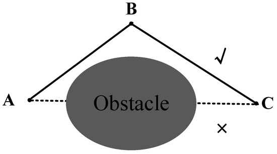
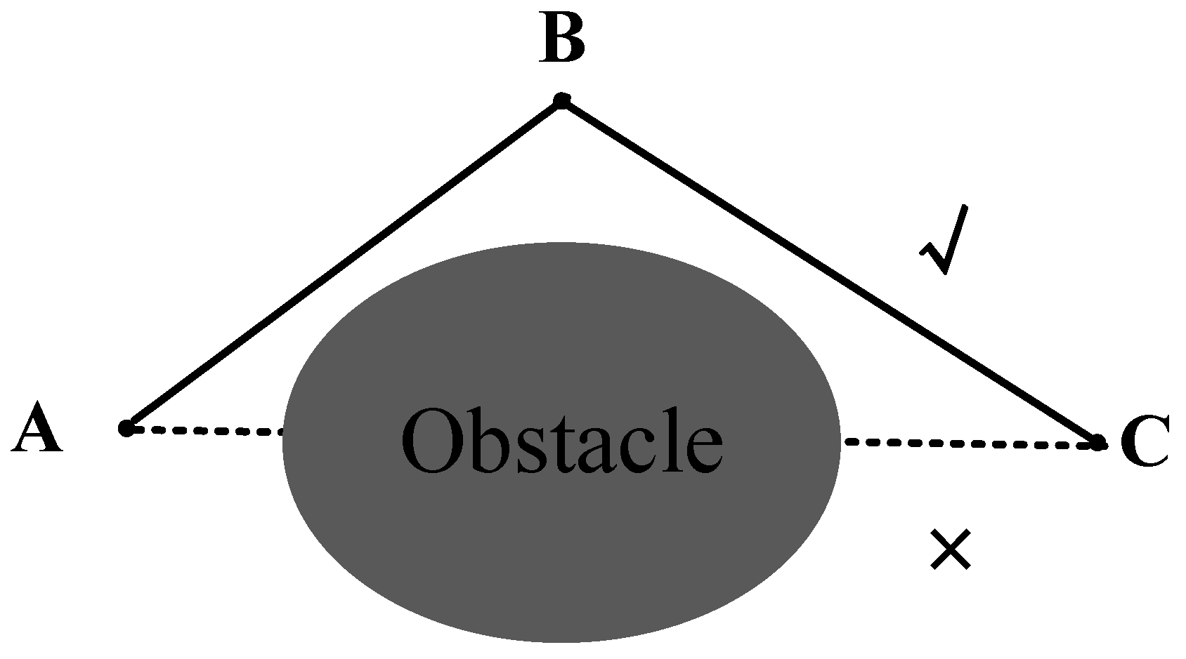
An illustrative example is shown in Figure 1, where A, B, and C denote path nodes. the line segment AC that intersects an obstacle is shown as a dashed line and marked with a cross (×) to indicate that such a path is infeasible; while the segments AB and BC are shown as solid lines and marked with a checkmark (√) nearby to indicate that they are acceptable.

2.2. Path–Smoothing Strategy for Adding Third–Order Bezier Curve

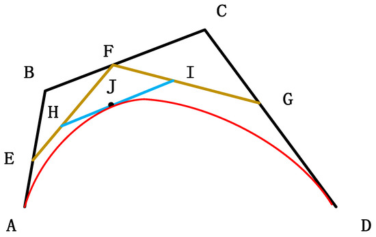
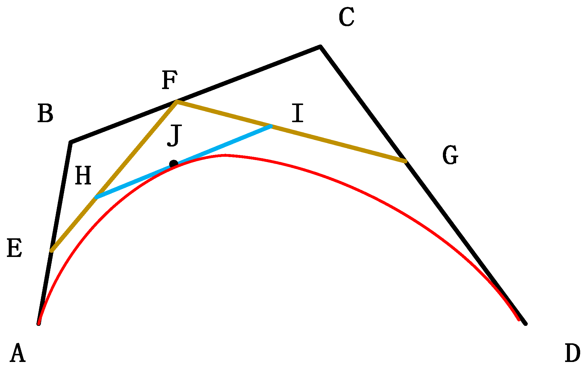
In the path generated by the above JPS algorithm, the output path is usually a number of end–to–end line segments, the path direction changes in a discrete mutation, and the curvature is discontinuous. In view of the advantages of continuous curvature, local support, simple calculation, and controllable smoothing strength of the third–order Bezier curve, the discrete broken line generated by the JPS can be transformed into a smooth and traceable path that satisfies the ASV kinematic constraints. In this section, the path–smoothing method based on the third–order Bezier curve is used to solve the problem of discreteness and curvature discontinuity in the output path. As shown in Figure 2, A, B, C, and D are control points, and a point E on AB, a point F on BC, and a point G on CD are taken to make AE/AB = BF/BC = CG/CD = $\alpha$; at the same time, a point H on EF, a point I on FG, and a point J on HI are taken to make EH/EF = FI/FG = HJ/HI = $\beta$. $\alpha$ and $\beta$ are the intermediate proportions in the generation process, and the final curve is determined by t, t ∈ [0, 1]. The set of all J points that meet the conditions is the generated Bezier curve, that is, the red line in the figure. The parameter equation is as follows:

B(t) = (1 − t)³P₀ + 3t(1 − t)²P₁ + 3t²(1 − t)P₂+ t³P₃

(3)

where P₀ represents point A, P₁ denotes point B, P₂ denotes point C, and P₃ denotes point D.

2.3. Simulation Verification of the Improved JPS Algorithm

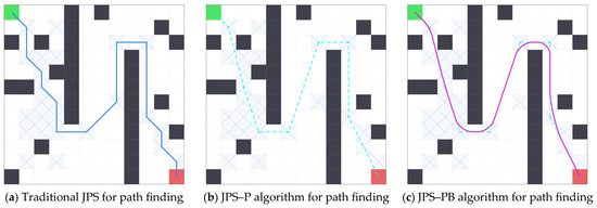
It should be noted that the JPS–PB proposed in this paper does not introduce a new path–smoothing theory; rather, to meet the requirements of global reference path generation for ASVs, it combines JPS jump–point search, line–of–sight–based redundant node removal, and third–order Bezier smoothing to improve the issues of path redundancy and curvature discontinuity in the original JPS algorithm. In this section, the improved JPS algorithm proposed above is referred to as JPS–PB, and the algorithm with only path pruning is referred to as JPS–P. The comparison experiments with the traditional JPS algorithm are shown in Figure 3. The green grids represent the start point, red grids represent the goal point, the path of the traditional JPS algorithm is shown as a blue solid line, and the path of the JPS–PB algorithm is shown as a red solid line. A 12 × 12 map is used, where black grids represent obstacles and white grids represent free space. The paths generated by the traditional JPS, JPS–P, and JPS–PB algorithms are shown as a blue solid line, a blue dashed line, and a purple solid line, respectively. The validation results include metrics such as path length, planning time, and total turning angle.

The simulation comparison results are shown in the

Table 1. Comparison of planning results.

Algorithm	Path Length s/m	Planning Time Consuming t/ms	Total Steering Angle ${\mathit{\theta }}_{\mathit{sum}}$/°	Maximum Steering Angle ${\mathit{\theta }}_{\mathit{max}}$/°
Traditional JPS	29.90	9.63	765.0	90.0
JPS–P	28.50	12.12	366.6	90.0
JPS–PB	27.32	12.72	316.4	10.3

:

Experimental results indicate that the path lengths generated by the conventional JPS, JPS–P, and JPS–PB algorithms are 29.90, 28.50, and 27.32, respectively. The redundant–node elimination strategy reduces the path length by 1.40, accounting for approximately 54.3% of the total reduction of 2.58. Subsequently, Bezier curve smoothing further shortens the path by 1.18, contributing the remaining 45.7% of the overall improvement. These results demonstrate that both strategies are effective in reducing path length, with redundant–node elimination providing a slightly greater contribution.

In terms of the maximum steering angle, both the conventional JPS and JPS–P algorithms exhibit a maximum turning angle of 90.0°, indicating that although redundant–node elimination effectively reduces unnecessary turning points, it does not alleviate abrupt heading changes at individual corners. After introducing Bezier curve smoothing, the maximum steering angle decreases dramatically from 90.0° to 10.3°, corresponding to a reduction of 88.6%. This improvement is almost entirely attributable to the Bezier–smoothing stage, highlighting its significant contribution to enhancing path continuity and local steering smoothness.

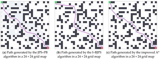
To further evaluate the performance of the proposed method, the I–BJPS algorithm [4] and the improved A* algorithm [5] were compared with the proposed JPS–PB algorithm. A 24 × 24 grid map, as illustrated in Figure 4, was constructed for the comparison, where the green cell denotes the start point, the red cell denotes the goal point, and the gray cells represent expanded nodes during the search process.

The performance comparison results of the three algorithms are summarized in

Table 2. Comparison of the results between the algorithm in References [4,5] and JPS–PB.

Algorithm	Path Length s/m	Planning Time Consuming t/ms	Total Steering Angle ${\mathit{\theta }}_{\mathit{sum}}$/°	Maximum Steering Angle ${\mathit{\theta }}_{\mathit{max}}$/°
JPS–PB	35.98	2.52	663.6	10.3
Algorithm in reference [4]	36.17	4.06	788.3	10.3
Algorithm in reference [5]	39.47	1.72	760.4	9.5

.

As shown in Table 2, the proposed JPS–PB algorithm exhibits superior overall performance in terms of path length and steering smoothness in the 24 × 24 grid environment. Compared with the method reported in Ref. [4], the path length generated by JPS–PB is reduced from 36.17 to 35.98, corresponding to a decrease of approximately 0.53%. Meanwhile, the planning time is reduced from 4.06 ms to 2.52 ms, representing an improvement of 37.9%, and the cumulative steering angle decreases from 788.3° to 663.6°, corresponding to a reduction of 15.8%. Both methods achieve the same maximum steering angle of 10.3°. These results indicate that JPS–PB is capable of generating shorter paths with lower cumulative steering effort and higher computational efficiency while maintaining the same maximum steering–angle constraint.

Compared with the method presented in Ref. [5], the path length obtained by JPS–PB decreases from 39.47 to 35.98, corresponding to a reduction of approximately 8.84%. In addition, the cumulative steering angle is reduced from 760.4° to 663.6°, yielding an improvement of 12.7%. These results demonstrate the clear advantage of JPS–PB in terms of path quality, as it effectively reduces unnecessary detours and overall steering effort. However, the algorithm in Ref. [5] only requires 1.72 ms for path planning, which is lower than the 2.52 ms required by JPS–PB, indicating a superior search efficiency. Furthermore, the maximum steering angle of Ref. [5] is 9.5°, slightly lower than the 10.3° achieved by JPS–PB, suggesting a marginal advantage in local maximum steering–angle control.

In summary, although JPS–PB does not achieve the best performance in every individual metric, it provides a favorable balance among path length, cumulative steering angle, and planning time. Compared with the method in Ref. [4], JPS–PB achieves improvements in path length, computational efficiency, and cumulative steering angle. Compared with the method in Ref. [5], JPS–PB exhibits slightly higher planning time and a marginally larger maximum steering angle but delivers significantly better path length and cumulative steering–angle performance. For global path planning of ASVs, path length and cumulative steering angle directly affect navigation distance, energy consumption, and path trackability. Therefore, JPS–PB is more suitable as a global reference path generator for subsequent local obstacle–avoidance modules.

In summary, the proposed JPS–PB algorithm significantly improves path smoothness and practical feasibility while maintaining high search efficiency. These characteristics make it particularly suitable for global path–planning tasks in large–scale and highly complex environments.

3. An Intelligent Path–Planning Algorithm Combining JPS–PB and Improved TEB Is Proposed

The JPS–PB algorithm generates a global reference path using prior environmental information. However, unknown obstacles and dynamic vessels in real maritime environments may still threaten navigation safety. Therefore, a local trajectory optimization strategy based on the TEB framework is introduced to enable real–time collision avoidance and trajectory adjustment.

3.1. Hull Modeling

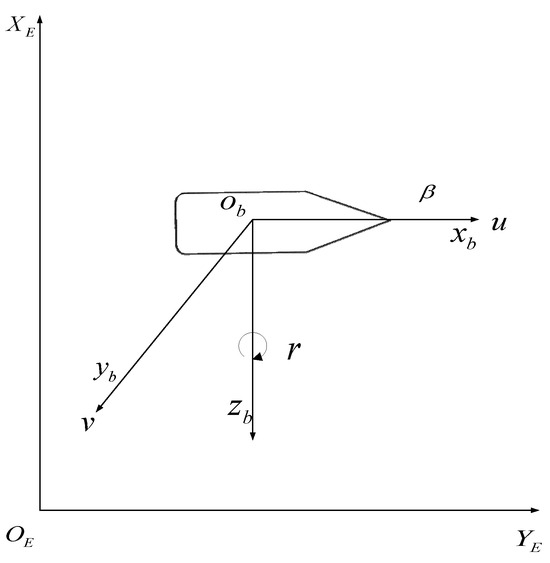
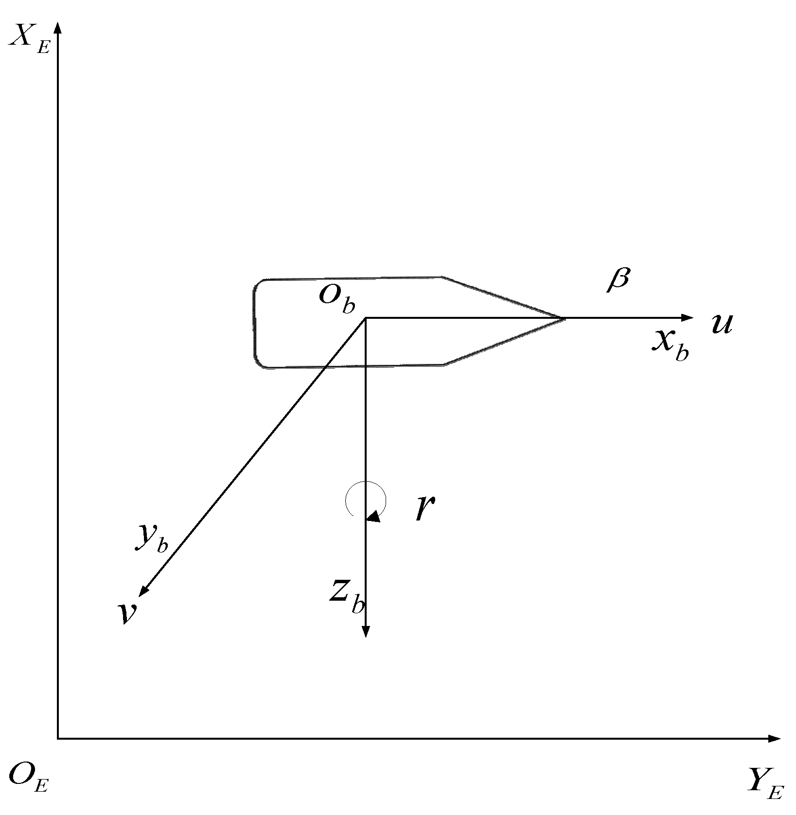
As shown in Figure 5, the geodetic coordinate system (${\mathit{O}}_{\mathit{E}}-{\mathit{X}}_{\mathit{E}}{\mathit{Y}}_{\mathit{E}}$) and the hull coordinate system (${\mathit{o}}_{\mathit{b}}-{\mathit{x}}_{\mathit{b}}{\mathit{y}}_{\mathit{b}}{\mathit{z}}_{\mathit{b}}$) are defined. The geodetic coordinate system takes a point on the surface of the Earth as the origin ${\mathit{O}}_{\mathit{E}}$. ${\mathit{O}}_{\mathit{E}}{\mathit{X}}_{\mathit{E}}$ point to the north of the geography, and ${\mathit{O}}_{\mathit{E}}{\mathit{Y}}_{\mathit{E}}$ point to the east of the geography. The hull coordinate system takes the center of gravity of the hull as the origin point ${\mathit{o}}_{\mathit{b}}$, ${\mathit{o}}_{\mathit{b}}{\mathit{x}}_{\mathit{b}}$ are parallel to the sea surface and point to the bow direction, ${\mathit{o}}_{\mathit{b}}{\mathit{y}}_{\mathit{b}}$ are parallel to the sea surface and point to the starboard direction, and ${\mathit{o}}_{\mathit{b}}{\mathit{z}}_{\mathit{b}}$ point to the Earth’s center and are perpendicular to the horizontal plane.

Since the TEB algorithm employed in this study primarily focuses on the planar pose of the ASV and its relative motion with respect to obstacle vessels, rather than the degrees of freedom that have a comparatively minor influence on collision–avoidance decision making, such as heave, roll, and pitch motions, only the surge, sway, and yaw motions in the horizontal plane are considered. Accordingly, the three–degree–of–freedom (3–DOF) mathematical model of the ASV in the horizontal plane can be expressed as follows. Let $\mathit{u}$ denote the surge velocity, $\mathit{v}$ the sway velocity, $\mathit{r}$ the yaw rate, and $\beta$ the heading angle of the ASV.

Only the surge, sway, and yaw motions in the horizontal plane are considered in the present study. The three–degree–of–freedom motion mathematical model of the ASV in the horizontal plane can be obtained. The ASV position and heading angle in the horizontal plane are defined as $\eta = {\left[\mathit{x},\mathit{y},\beta \right]}^{\mathrm{T}}$, and the speed is $\mathit{v} ={ \left[\mathit{u},\mathit{v},\mathit{r}\right]}^{\mathrm{T}}$. Assuming that the ASV is symmetrical about the middle longitudinal section and asymmetrical about the middle transverse section, the three–degree–of–freedom model of the ASV can be defined according to the above parameters.

$$\dot{\eta }=\mathit{J}\left(\beta \right)\mathit{v}$$

(4)

$$\mathit{J}(\beta )=\left[\begin{array}{ccc}\cos \beta & -\sin \beta & 0\\ \sin \beta & \cos \beta & 0\\ 0& 0& 1\end{array}\right]$$

(5)

3.2. TEB Path Planning Considering COLREGs

The optimization object of the TEB algorithm is n, which is closely related to the pose points and the time interval between the adjacent pose points. It is essentially a multi–objective constrained optimization problem. The objective function integrates various constraint costs by weighted summation. The optimization objective is to minimize the total cost function to obtain the optimal trajectory $B^{\ast }$. The mathematical expression is as follows:

$$\mathit{f}\left(\mathit{B}\right) ={\sum }_{\mathit{k}}{\gamma }_{\mathit{k}}{\mathit{f}}_{\mathit{k}}\left(\mathit{B}\right)$$

(6)

$${\mathit{B}}^{\ast }=\arg \underset{\mathit{B}}{\min }\mathit{f}\left(\mathit{B}\right)$$

(7)

In the above formula, $\mathit{f}\left(\mathit{B}\right)$ is the total objective function considering various constraints, ${\gamma }_{\mathit{k}}$ is the weight coefficient of each sub–cost function to adjust the priority and weight of different constraints, ${\mathit{f}}_{\mathit{k}}\left(\mathit{B}\right)$ is the sub–cost function corresponding to various constraints, and $B^{\ast }$ represents the optimal trajectory. The specific calculation method is detailed in Reference [9].

Assuming that the position of the ship is $(\mathit{x},\mathit{y},\beta )$ and the position of the target ship is $({\mathit{x}}_0,{\mathit{y}}_0)$, then the relative phase angle $\varphi$ is calculated as follows:

$$\varphi = \mathit{atan}2({\mathit{y}}_0-\mathit{y},{\mathit{x}}_0-\mathit{x})-\beta$$

(8)

To ensure that phi lies within (−180 deg, 180 deg), it is normalized as follows:

$$\varphi = \left(\right({\varphi }_{\mathit{raw}}+180°)\mathit{mod} 360°)-180°$$

(9)

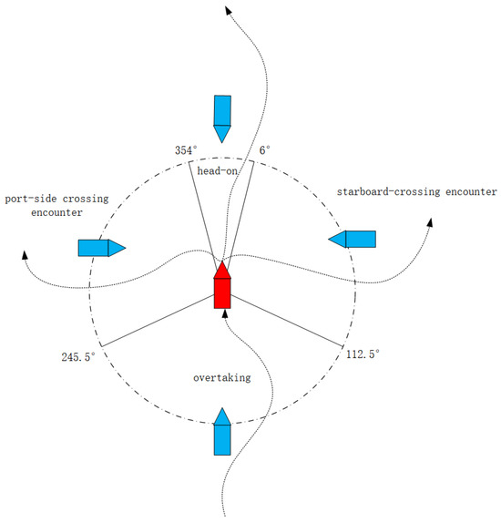
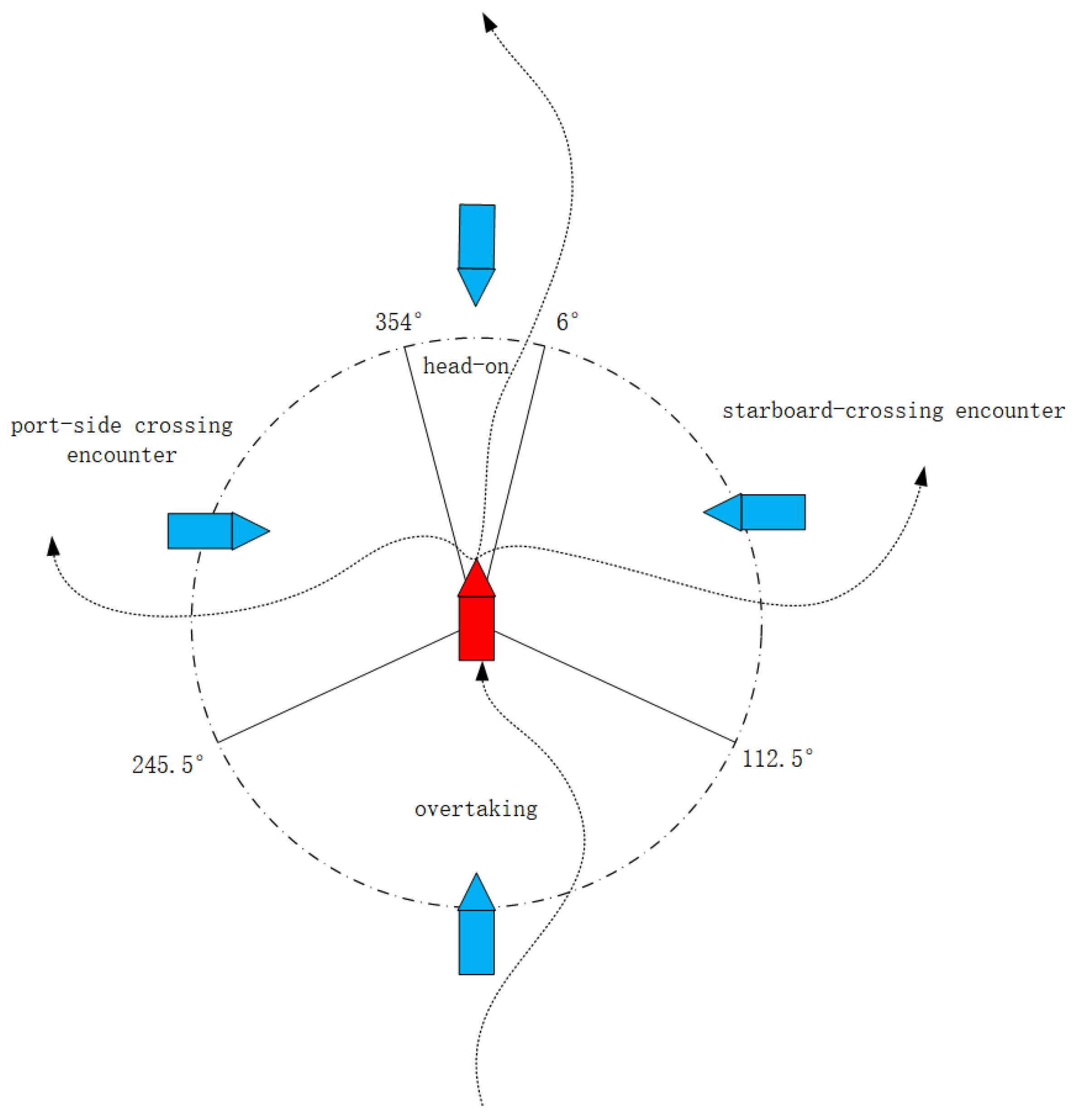
Define the head–on angle as ${\varphi }_{\mathit{h}} = 6°$ and the crossing angle as ${\varphi }_{\mathit{c}} = 112.5°$. Figure 6 shows the own vessel (red), the target obstacle vessel (blue), and the dashed line representing the COLREGs–compliant path of the own vessel. When $\left|\varphi \right| \le {\varphi }_{\mathit{h}}$, it is a head–on situation, and the own vessel should turn to starboard. When ${\varphi }_{\mathit{c}} < \varphi <{ \varphi }_{\mathit{h}}$, it is a starboard–crossing encounter situation, and the own vessel, as the give–way vessel, should turn to starboard. When ${-\varphi }_{\mathit{h}} < \varphi { < -\varphi }_c$, it is a special port–side–crossing encounter situation, and the own vessel, as the stand–on vessel, should maintain course and speed. However, in special circumstances, such as when the give–way vessel in a special port–side–crossing encounter fails to take avoidance action, the own vessel should turn to port to pass astern of the target vessel. When the own vessel is the overtaking vessel and $\left|\varphi \right| \le \left|{\varphi }_{\mathit{c}}-90°\right|$, the COLREGs do not explicitly require passing on a specific side, but it is recommended to pass astern of the overtaking vessel; therefore, it is advised to turn in the direction opposite to the overtaking vessel. If the own vessel and the target obstacle vessel move in the same direction, it is recommended that the own vessel turn to the side away from the target obstacle vessel. According to the COLREGs requirements considered in this study, where the own vessel is explicitly required to turn to starboard, and special port–side–crossing encounter situations in which the own vessel is the stand–on vessel and should maintain course and speed, the own vessel should turn in the direction opposite to the motion of the target obstacle vessel in all other cases.

For special cases such as a special port–side–crossing encounter, in which the give–way vessel fails to take action, it is insufficient to only consider the turning requirement specified by the collision regulations; safety distance must also be considered. Therefore, a smooth gating function is introduced as a switch to activate the collision–avoidance function. The relevant definitions are as follows:

The position vector of the ship relative to the target obstacle ship is r = [x − ${\mathit{x}}_0$ y − ${\mathit{y}}_0$], and the velocity vector of the target obstacle ship is ${\mathit{v}}_0=\left({\mathit{v}}_{\mathit{ox}}, {\mathit{v}}_{oy}\right)$. In order to calculate the relative azimuth, this method defines the cross product z component of r and ${\mathit{v}}_0$ as c as follows:

$$c= r \times {\mathit{v}}_0= (\mathit{x} - {\mathit{x}}_0) {\mathit{v}}_{\mathrm{o}\mathrm{y}}- (\mathit{y} - {\mathit{y}}_0) {\mathit{v}}_{\mathit{ox}}$$

(10)

The symbol indicates the ship’s lateral position relative to the course of the target ship: c > 0 when the ship is on the left side of the target ship and c < 0 when the ship is on the right side of the target ship.

If the ship speed is defined as ${\mathit{v}}_{\mathit{k}}$, then the speed vector relative to the target ship is as follows:

$${\mathit{v}}_{0,\mathit{k}}={\mathit{v}}_{\mathit{k}}-{\mathit{v}}_0$$

(11)

The position of the two ships in relative motion can be expressed as follows:

$${r\left(\mathit{t}\right)=r}_k+{\mathit{v}}_{0,\mathit{k}}\mathit{t}$$

(12)

The square of its distance is as follows:

$${\mathit{D}}^2\left(\mathit{t}\right) = {‖\mathit{r}\left(\mathit{t}\right)‖}^2 = {({\mathit{r}}_{\mathit{k}} +{ \mathit{v}}_{0,\mathit{k}}\mathit{t})}^{\mathit{T}}({\mathit{r}}_{\mathit{k}} +{ \mathit{v}}_{0,\mathit{k}}\mathit{t})$$

(13)

Expand to get

$${\mathit{D}}^2\left(\mathit{t}\right)={‖{\mathit{r}}_{\mathit{k}}‖}^2+2({{\mathit{r}}_{\mathit{k}}}^{\mathit{T}}{\mathit{v}}_{0,\mathit{k}})\mathit{t}+{‖{\mathit{v}}_{0,\mathit{k}}‖}^2{\mathit{t}}^2$$

(14)

In order to find the most recent meeting moment, the derivation of ${\mathit{D}}^2\left(\mathit{t}\right)$ is obtained as follows:

$${\displaystyle \frac{\mathit{d}{\mathit{D}}^2\left(\mathit{t}\right)}{\mathrm{dt}}} = 2{{\mathit{r}}_{\mathit{k}}}^{\mathit{T}}{\mathit{v}}_{0,\mathit{k}} + {2‖{\mathit{v}}_{0,\mathit{k}}‖}^2\mathit{t}$$

(15)

In order to get the closest approach time, let the derivative be zero, then there is

$$2{{\mathit{r}}_{\mathit{k}}}^{\mathit{T}}{\mathit{v}}_{0,\mathit{k}}+{2‖{\mathit{v}}_{0,\mathit{k}}‖}^2\mathit{t}=0$$

(16)

The closest approach time is

$${\mathrm{TCPA}}_{\mathit{k}}=-{\displaystyle \frac{{{\mathit{r}}_{\mathit{k}}}^{\mathit{T}}{\mathit{v}}_{0,\mathit{k}}}{{‖{\mathit{v}}_{0,\mathit{k}}‖}^2}}$$

(17)

The nearest encounter distance obtained by substituting the nearest encounter time is as follows:

$${\mathrm{DCPA}}_{\mathit{k}}=‖{\mathit{r}}_{\mathit{k}} +{ \mathrm{TCPA}}_{\mathit{k}}{\mathit{v}}_{0,\mathit{k}}‖$$

(18)

Considering that the maritime collision–avoidance rules are only considered when two ships are close to each other, in order to activate the rule cost in the presence of such collision risk, the smooth gate control function is introduced by extending the Sigmoid function $\sigma \left(\mathit{z}\right)$:

$${ \gamma }_{\mathit{k}}=\sigma \left({\displaystyle \frac{{\mathit{D}}_{\mathit{t}\mathit{h}} -{ \mathrm{DCPA}}_{\mathit{k}}}{{\mathit{s}}_{\mathit{d}}}}\right)·\sigma \left({\displaystyle \frac{{\mathrm{TCPA}}_{\mathit{k}}}{{\mathit{s}}_t}}\right)·\sigma \left({\displaystyle \frac{T_{\mathit{th}}- {\mathrm{TCPA}}_{\mathit{k}}}{{\mathit{s}}_t}}\right)$$

(19)

where ${\mathsf{\gamma }}_{\mathit{k}} \in (0, 1)$ is the risk activation coefficient, ${\mathit{D}}_{\mathit{t}\mathit{h}}$ is the hazard distance threshold, $T_{\mathit{th}}$ is the hazard time threshold, ${\mathit{s}}_{\mathit{d}}$ and ${\mathit{s}}_{\mathit{t}}$ are the smoothing coefficients, and $\sigma \left(\mathit{z}\right) = {(1+{\mathrm{e}}^{-\mathrm{z}})}^{-1}$. When ${\mathrm{DCPA}}_{\mathit{k}}<{\mathit{D}}_{\mathit{t}\mathit{h}}$, the first item tends to be 1, indicating that the target obstacle ship enters the danger threshold range. When ${\mathrm{TCPA}}_{\mathit{k}}>0$, the second term approaches 1, indicating that the collision occurs in the future rather than in the past. When ${\mathrm{TCPA}}_{\mathit{k}}<T_{\mathit{th}}$, it means that the collision risk occurs in the foreseeable time window. Therefore, the closer ${\gamma }_{\mathit{k}}$ is to 1, the stronger the risk is, the more obvious the corresponding cost is.

Thus, in a special port–side–crossing encounter, if the target obstacle vessel takes effective avoidance action, the risk activation coefficient approaches 0, the collision–avoidance function is not activated, and the own vessel maintains its original course and speed as the stand–on vessel. If the target obstacle vessel fails to take effective avoidance action, the risk activation coefficient approaches 1, the collision–avoidance function is activated, and the own vessel acts as the give–way vessel by moving in the opposite direction to the target obstacle vessel in order to pass astern of it. By introducing this mechanism, both the behavior of the own vessel as the stand–on vessel and its behavior as the give–way vessel in special cases are defined.

The collision–avoidance function ${\mathit{f}}_{\mathit{col}}$ is defined as follows:

To represent the left–right position of the target ship in the local coordinate system of the own vessel, the lateral positional offset is defined as follows:

$${\mathit{e}}_{\mathit{k}} = [-\sin {\beta }_{\mathit{k}} \cos {\beta }_{\mathit{k}}]\left[\begin{array}{c}{\mathit{x}}_0-{\mathit{x}}_{\mathit{k}}\\ {\mathit{y}}_0-{\mathit{y}}_{\mathit{k}}\end{array}\right]$$

(20)

To represent the left–right direction of the target obstacle vessel’s motion in the local coordinate system of the own vessel, the lateral velocity offset is defined as follows:

$${\mathit{v}}_{0,\mathrm{lat}} = [-\sin {\beta }_{\mathit{k}} \cos {\beta }_{\mathit{k}}]\left[\begin{array}{c}{\mathit{v}}_{\mathit{ox}}\\ {\mathit{v}}_{\mathit{oy}}\end{array}\right]$$

(21)

where $[-\sin {\beta }_{\mathit{k}} \cos {\beta }_{\mathit{k}}]$ is the direction vector of the own vessel’s local coordinate frame pointing to the port side. When ${\mathit{e}}_{\mathit{k}} > 0$, the target ship is located on the port side of the own vessel; when ${\mathit{e}}_{\mathit{k}} < 0$, it is located on the starboard side. Similarly, when ${\mathit{v}}_{0,\mathrm{lat}} > 0$, the target ship’s velocity is directed toward the port side of the own vessel; when ${\mathit{v}}_{0,\mathrm{lat}} < 0$, it is directed toward the starboard side.

Similarly, to represent the forward–backward component of the target obstacle vessel’s motion in the local coordinate system of the own vessel, the longitudinal velocity offset is defined as:

$${\mathit{v}}_{0,\mathrm{lon}} = [\cos {\beta }_{\mathit{k}} \sin {\beta }_{\mathit{k}}]\left[\begin{array}{c}{\mathit{v}}_{\mathit{ox}}\\ {\mathit{v}}_{\mathit{oy}}\end{array}\right]$$

(22)

where $[\cos {\beta }_{\mathit{k}} \sin {\beta }_{\mathit{k}}]$ is the unit vector along the own–ship heading. When ${\mathit{v}}_{0,\mathrm{lon} }> 0$, the target obstacle vessel moves toward the forward direction of the own vessel; when ${\mathit{v}}_{0,\mathrm{lon}} < 0$, it moves toward the aft direction.

The desired turning direction is defined as ${\mathit{d}}_{\mathrm{des}}\in \{-1,0,1\}$, where ${\mathit{d}}_{\mathrm{des}}$ = −1 indicates that the own vessel should turn to port, ${\mathit{d}}_{\mathrm{des}}$ = 1 indicates that it should turn to starboard, and ${\mathit{d}}_{\mathrm{des}}$ = 0 indicates that it should maintain course.

According to the preceding discussion, in head–on encounters, ${\mathit{d}}_{\mathrm{des}}$ = 1. In other cases, to ensure that the own vessel moves away from the obstacle vessel, the following sign function $\mathit{sgn}\left(\mathit{x}\right)$ is introduced:

$${\mathit{d}}_{\mathrm{des}} = -\mathit{sgn}\left({\mathit{v}}_{0,\mathrm{lat}}\right)$$

(23)

This expression indicates that when ${\mathit{v}}_{0,\mathrm{lat}} > 0$, ${\mathit{d}}_{\mathrm{des}} < 0$; when ${\mathit{v}}_{0,\mathrm{lat}} < 0$, ${\mathit{d}}_{\mathrm{des}} > 0$. That is, when the obstacle vessel moves toward the right, the own vessel should turn to port; when it moves toward the left, the own vessel should turn to starboard. This is consistent with starboard–crossing encounters, as well as with the special case of the port–side–crossing encounter in which the give–way vessel fails to take effective avoidance action.

When ${\mathit{v}}_{0,\mathrm{lat}} = 0$ and the situation is overtaking, to ensure safety and steer the own vessel away from the obstacle vessel, the following similar sign function $\mathit{sgn}\left(\mathit{x}\right)$ is used:

$${\mathit{d}}_{\mathrm{des}} = -\mathit{sgn}\left({\mathit{e}}_{\mathit{k}}\right)$$

(24)

This expression indicates that, when the own vessel and the obstacle vessel sail in the same direction, ${\mathit{e}}_{\mathit{k}} > 0$, and ${\mathit{d}}_{\mathrm{des}} < 0$; if ${\mathit{e}}_{\mathit{k}} < 0$, then ${\mathit{d}}_{\mathrm{des}} > 0$. That is, when the obstacle vessel is on the starboard side of the own vessel, the own vessel turns to port, and vice versa. Although COLREGs do not mandate a particular side for overtaking, for safety reasons, the own vessel should actively move away from the obstacle vessel to avoid risking a collision. Therefore, when the obstacle vessel is on the starboard side, the own vessel turns to port; when it is on the port side, it turns to starboard, thereby increasing the lateral separation between the vessels. Considering that environmental disturbances, such as wind, waves, and currents, are ubiquitous in real marine environments, the case in which both ${\mathit{v}}_{0,\mathrm{lat}}$ and ${\mathit{e}}_{\mathit{k}}$ are simultaneously zero is practically non–existent and is therefore not discussed.

Considering that Equations (23) and (24) have similar forms, they are unified as follows:

$${\mathit{d}}_{\mathrm{des}}=-\mathit{sgn}\left(\mathit{g}\right)$$

(25)

The value of g is taken as follows:

$$\mathit{g} = \left\{\begin{array}{c}{\mathit{v}}_{0,\mathrm{lat}}, {\mathit{v}}_{0,\mathrm{lat}} \ne 0\\ {\mathit{e}}_{\mathit{k}}, {\mathit{v}}_{0,\mathrm{lat}} = 0\end{array}\right.$$

(26)

After summarizing all encounter situations, the formula for ${\mathit{d}}_{\mathrm{des}}$ is given as follows:

$${\mathit{d}}_{\mathrm{des}}=\left\{\begin{array}{c}1, \left|\varphi \right| \le {\varphi }_{\mathit{h}} and {\mathit{v}}_{0,\mathrm{lon}} < 0 \\ -\mathit{sgn}\left(\mathit{g}\right), \mathrm{otherwise}\hfill \end{array}\right.$$

(27)

Accordingly, the cost function can be reformulated as follows:

$${\mathit{f}}_{\mathit{col}}={\gamma }_{\mathit{k}}\max (0,-{\mathit{d}}_{\mathrm{des}}△\beta )$$

(28)

$△\beta$ denotes the current yaw–rate of the own vessel; $△\beta > 0$ indicates clockwise rotation, while $△\beta < 0$ indicates counter–clockwise rotation. When the own vessel turns in the expected direction, d_des and $△\beta$ have the same sign (both positive or both negative), i.e., ${\mathit{d}}_{\mathrm{des}}△\beta > 0$. In this case, $\max (0,-{\mathit{d}}_{\mathrm{des}}△\beta )$ = 0, so ${\mathit{f}}_{\mathit{col}}$ = 0. When the own vessel does not turn in the expected direction, ${\mathit{d}}_{\mathrm{des}}△\beta < 0$, and consequently ${\mathit{f}}_{\mathit{col}} ={ \gamma }_{\mathit{k}}-{\mathit{d}}_{\mathrm{des}}△\beta$. In this situation, the constraint is violated, and the cost function f_col yields a positive value, which, during optimization, encourages the own vessel to adjust its yaw rate, $△\beta$, so that it has the same sign as the desired turning direction, d_des, thereby achieving the turning behavior that is compliant with the COLREGs.

The collision–regulation cost function ${\mathit{f}}_{\mathit{col}}$ is incorporated into the total objective function of TEB through the weight ${\gamma }_{col}$ as follows:

$$\mathit{f}\left(\mathit{B}\right)={\sum }_{\mathit{k}}{\gamma }_{\mathit{k}}{\mathit{f}}_{\mathit{k}}\left(\mathit{B}\right)+{\gamma }_{col}{\mathit{f}}_{\mathit{col}}\left(\mathit{B}\right)$$

(29)

It should be noted that our COLREGs implementation, particularly Rule 17, is simplified for typical single–vessel encounters (head–on, crossing, and overtaking). The DCPA/TCPA–based risk activation provides a practical threshold for stand–on vessel action when the give–way vessel fails to maneuver. However, we do not claim to cover all COLREGs complexities or multi–vessel interactions. Our aim is to demonstrate a feasible integration of rule constraints into TEB under common operational conditions.

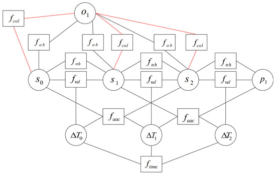
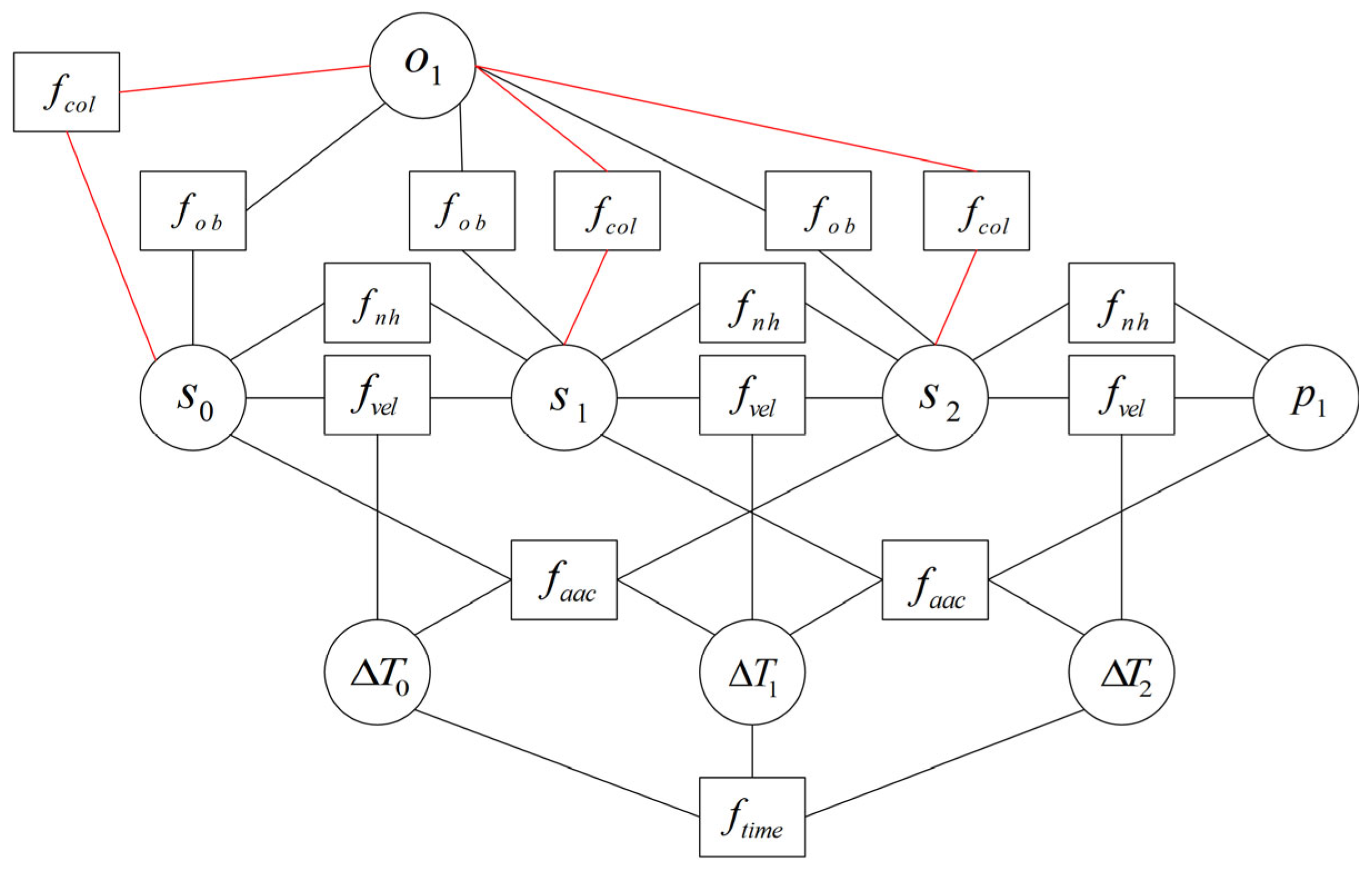
In this paper, the TEB algorithm, which integrates the rules of collision avoidance at sea, is called CTEB for short. The algorithm takes the pose point, time, obstacle, and waypoint as nodes, the constraint function as the edge, and relies on the g2o framework and interpreter to solve [20,21]. The hypergraph after adding the collision–avoidance strategy is shown in Figure 7.

Among them, ${\mathrm{s}}_1$ and ${\mathrm{s}}_2$ are the pose points that are optimized and adjusted, and the obstacle ${\mathrm{o}}_1$ and the waypoint ${\mathrm{s}}_0$ and ${\mathrm{p}}_1$ are not optimized and have not been changed. The black line represents the content of the traditional TEB algorithm hypergraph, and the red line is the newly added maritime collision–avoidance rule constraint.

The key variables and parameters appearing in the above sections are summarized in

Table 3. Table of key parameters.

Category	Parameter	Definition	Value	Unit	Justification
COLREGs determination	ϕh	Head–on angle threshold	6	°	Based on international practice
	${\varphi }_{\mathit{c}}$	Crossing angle threshold	112.5	°
Risk activation	${\mathit{D}}_{\mathit{t}\mathit{h}}$	Dangerous encounter distance threshold	5	m	Based on international practice
	${\mathit{T}}_{\mathit{th}}$	Dangerous encounter time threshold	6	s
	${\mathit{s}}_{\mathit{d}}$	Smoothing coefficient (distance)	2	m
	${\mathit{s}}_{\mathit{t}}$	Smoothing coefficient (time)	1	s
Cost function weight	${\gamma }_{col}$	COLREGs cost weight	5–40	–	Determined according to hull length and speed in the experiments

.

3.3. Time Complexity Analysis

Compared with the conventional TEB algorithm, the proposed CTEB introduces additional components, including COLREGs–based encounter classification, a risk activation function, and a rule–based steering cost function, on top of the original kinematic, velocity, acceleration, and obstacle–distance constraints. Consequently, the primary increase in computational complexity arises from the calculation of the relative bearing between the own vessel and the dynamic obstacle vessels, the evaluation of the DCPA, TCPA, and the determination of the desired steering direction.

CTEB formulates local trajectory optimization as a sparse hyper–graph optimization problem. Let n denote the number of pose states within the optimization horizon, m the number of dynamic obstacles, and q the number of optimization iterations. Since the state dimension of each pose remains constant, the computational complexity of the conventional TEB algorithm can be expressed as follows:

$${\mathit{T}}_{\mathit{TEB}} = \mathit{O}\left(\mathit{qnm}\right)$$

(30)

In CTEB, additional constraints are incorporated, including COLREGs encounter–type classification, TCPA and DCPA evaluation, the risk activation function, and the rule–based steering cost function. Since all of these newly introduced operations require only constant–time computations, the additional computational overhead can be represented as follows:

$$\mathit{O}(∆\mathit{qnm})$$

(31)

where $∆$ denotes the constant–factor increase introduced by the COLREGs–related constraints.

Therefore, the overall computational complexity of CTEB can be expressed as follows:

$${\mathit{T}}_{\mathit{CTEB}} = \mathit{O}\left(\right(1 + ∆) \mathit{qnm})$$

(32)

It can be observed that CTEB and the conventional TEB algorithm share the same asymptotic time complexity. Since the COLREGs–related constraints only introduce constant–time operations, such as relative–bearing calculation, TCPA, DCPA evaluation, and rule–based cost assessment, the additional computational burden is reflected solely in the constant factor of the complexity expression. As a result, the actual computational cost per iteration increases slightly, while the asymptotic complexity remains unchanged.

In practical applications, the number of pose states $\mathit{n}$, dynamic obstacles $\mathit{m}$, and optimization iterations $\mathit{q}$ are typically bounded within a limited range. Therefore, the proposed CTEB algorithm remains capable of satisfying the real–time requirements of online path planning for ASVs.

3.4. Fusion Path Planning of JPS–PB and Improved TEB

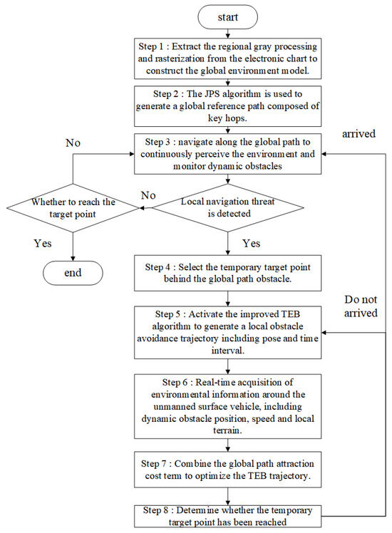
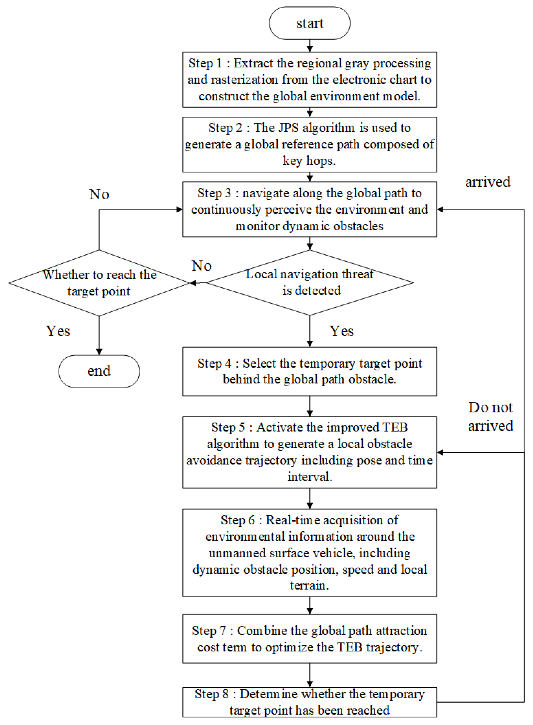
Global path planning relies on a priori environment, lacks real–time responsiveness, and cannot effectively handle dynamic obstacles. The local planning based on CTEB is flexible and real–time, but it is easy to fall into a local optimum due to the influence of the initial solution, resulting in path oscillation, and it is easy to deviate from the optimal route when there is no global guidance. Therefore, this paper integrates JPS–PB and CTEB, and proposes a fusion path–planning strategy: first, the global optimal path is generated by JPS–PB; during the navigation, the environment is monitored by sensors, and when dynamic obstacles or other threats that do not meet the basic constraints are detected, the CTEB is switched to local obstacle avoidance; after obstacle avoidance, smoothly return to the original global path and continue to sail to the target. The specific steps are shown in Figure 8.

4. Emulation Testing

4.1. Performance Evaluation of the CTEB Algorithm

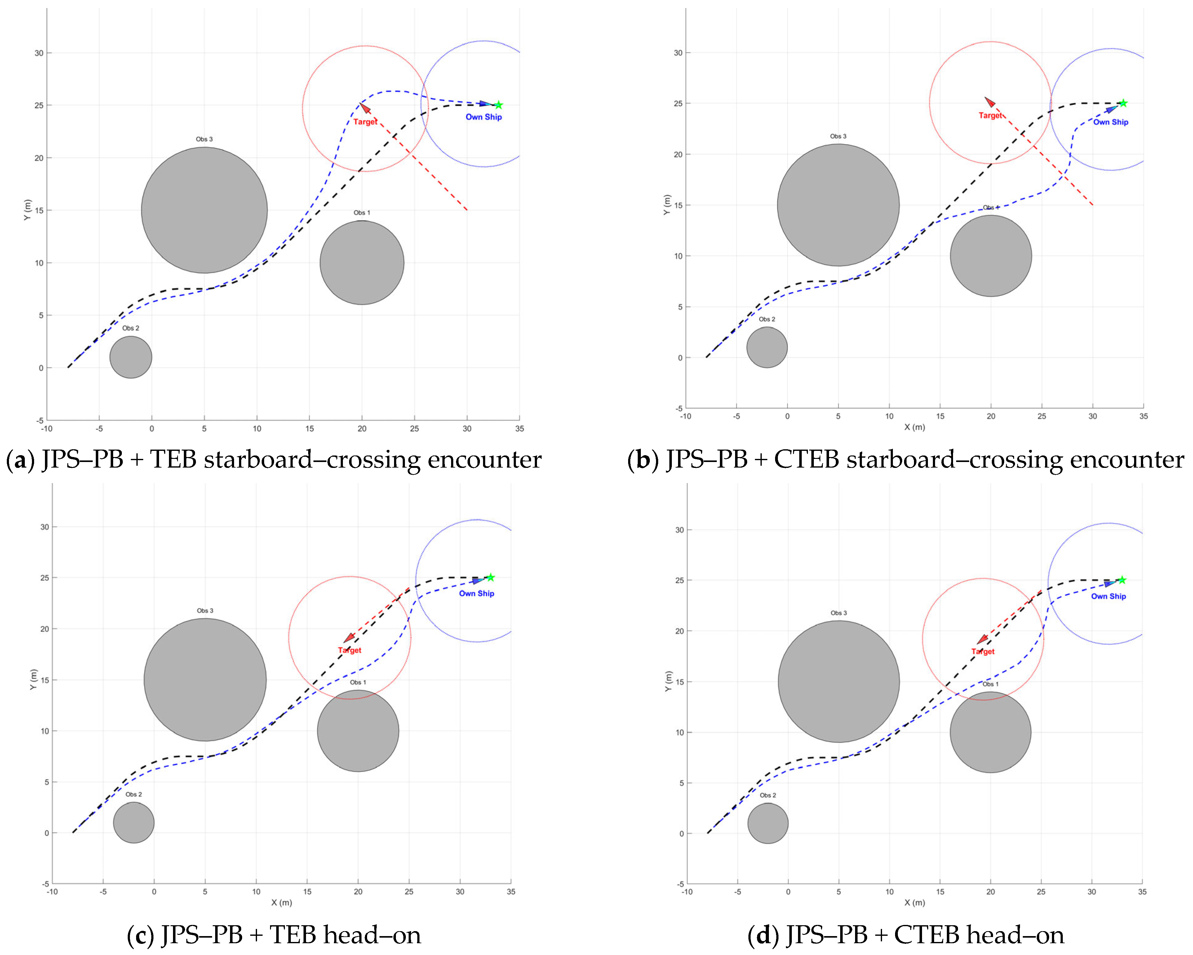
In this section, the proposed JPS–PB algorithm is integrated with both the conventional TEB and the proposed CTEB algorithms for simulation–based evaluation. Static obstacles in the environment are used to represent maritime islands, whereas dynamic obstacles are employed to simulate surrounding vessels. The simulation map is first discretized into grid cells. Subsequently, the global reference path generated by JPS–PB is illustrated as a black dashed line, while the actual trajectory generated by the local planner is represented by a blue dashed line.

The own vessel is modeled as a blue triangular marker with an initial position of (−8,0), a target position of (33,25), an initial heading of 45°, and a cruising speed of 2.5 m/s. The safety distance is set to 5 m. Other vessels are represented by red triangular markers. The length of the own vessel is assumed to be 1.5 m. Following the DCPA, TCPA–based collision–risk assessment framework proposed by Woo and Kim [22], and considering the vessel dimensions, navigation speed, and local–planning range adopted in this study, the risk–assessment parameters are selected as ${\mathit{D}}_{\mathit{t}\mathit{h}} = 5,{ \mathit{T}}_{\mathit{th}} = 6,{ \mathit{s}}_{\mathit{d}} = 2,{ \mathit{s}}_{\mathit{t}} = 1, {\gamma }_{\mathit{col}} = 20$.

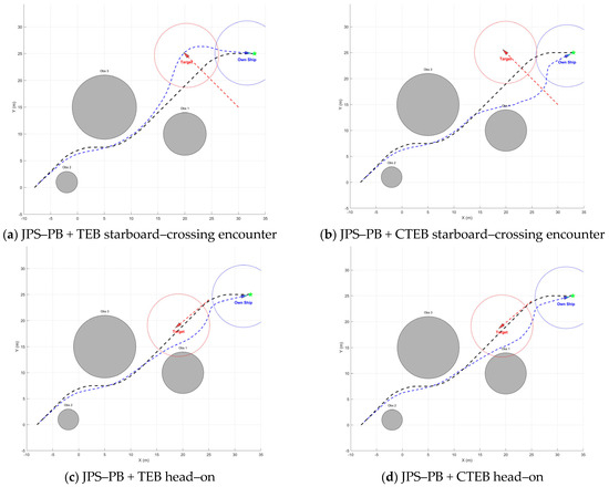
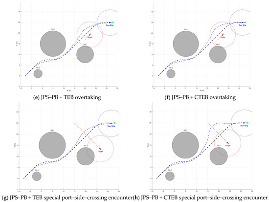
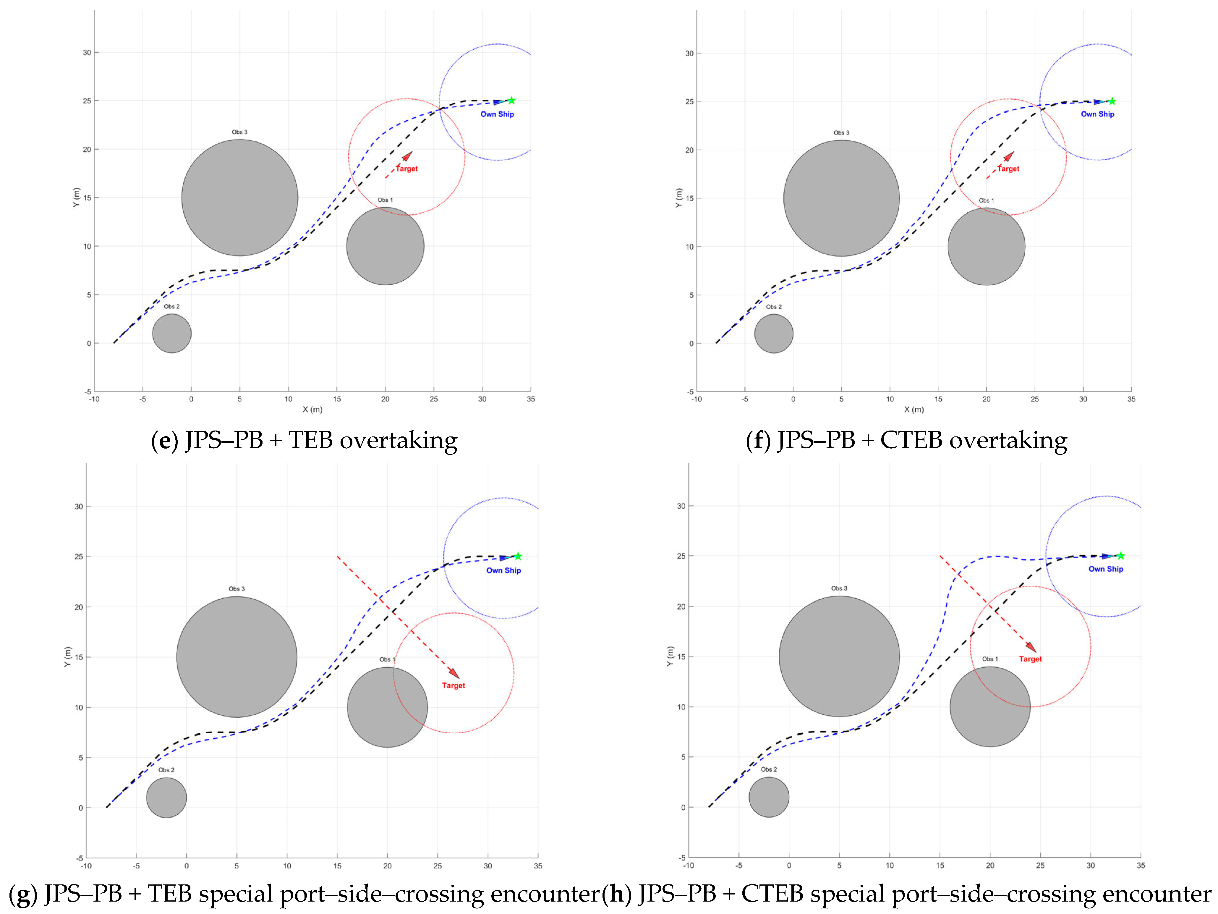
Four representative encounter scenarios requiring active collision–avoidance maneuvers are considered, including a starboard–crossing encounter, an overtaking encounter, a head–on encounter, and a special port–side–crossing encounter in which the give–way vessel fails to take appropriate avoidance action, as illustrated in Figure 9. The black dashed line represents the global path generated by JPS–PB, and the blue and red dashed lines indicate the actual trajectories of the blue vessel and the red vessel, respectively.

Starboard–crossing encounter:

The target vessel is initially located at (30,15) with a speed of 0.2 m/s and a heading of 135°. According to COLREGs, the own vessel acts as the give–way vessel and should alter course to starboard to pass astern of the target vessel.

As shown in Figure 9a, the conventional TEB algorithm generates a trajectory that passes ahead of the target vessel by turning to port when the encounter occurs near (17.5,20), thereby violating the recommended COLREGs maneuver. In contrast, the proposed CTEB algorithm, shown in Figure 9b, identifies the encounter correctly and performs a starboard maneuver near (21,15), allowing the own vessel to pass safely behind the target vessel. Compared with TEB, the CTEB–generated trajectory remains farther from the obstacle vessel and avoids crossing its forward motion direction, resulting in a safer and COLREGs–compliant navigation behavior.

Head–On Encounter:

The target vessel is initialized at (25,24) with a speed of 0.2 m/s and a heading of −140°. According to COLREGs, both vessels should alter course to starboard.

As illustrated in Figure 9c, the conventional TEB algorithm performs a starboard maneuver when the two vessels approach each other near (13,12.5), allowing the own vessel to pass safely on the port side of the obstacle vessel. Similarly, the proposed CTEB algorithm, shown in Figure 9d, correctly classifies the situation as a head–on encounter based on the relative bearing and motion directions. The rule–based cost function encourages a smoother and more pronounced starboard maneuver, resulting in a greater separation distance from the target vessel. Consequently, the CTEB trajectory provides a higher level of navigational safety than that generated by the conventional TEB algorithm.

Overtaking Encounter:

The target vessel is initially positioned at (20,17) with a speed of 0.1 m/s and a heading of 45°. Since the own vessel travels at a higher speed, an overtaking situation is formed. According to COLREGs, the overtaking vessel bears full responsibility for collision avoidance and should avoid cutting across the bow of the overtaken vessel.

As shown in Figure 9e, the conventional TEB algorithm generates a trajectory that passes close to the target vessel. In contrast, the proposed CTEB algorithm, shown in Figure 9f, determines that the obstacle vessel is located on the starboard side while moving in a similar direction. Consequently, the rule–based steering cost penalizes starboard–side intrusion and guides the own vessel to safely overtake on the port side. Compared with the conventional TEB trajectory, the CTEB trajectory maintains a larger clearance distance and exhibits improved safety.

Special port–side–crossing encounter:

In this scenario, the target vessel is initially located at (15,25) with a speed of 0.2 m/s and a heading of −45°. The vessel approaching from the port side fails to take effective collision–avoidance action. Under these special circumstances, the own vessel must assume collision–avoidance responsibility and avoid passing ahead of the target vessel.

As illustrated in Figure 9g, the conventional TEB algorithm generates a trajectory that passes on the starboard side of the obstacle vessel. By contrast, the proposed CTEB algorithm, shown in Figure 9h, introduces a penalty for starboard maneuvers through the rule–based steering function, thereby encouraging a port–side maneuver and enabling the own vessel to pass safely astern of the target vessel. Compared with the conventional TEB trajectory, the CTEB–generated route maintains a larger separation distance and provides improved collision–avoidance performance.

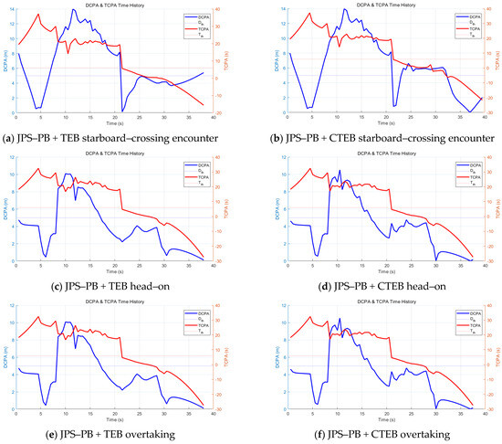
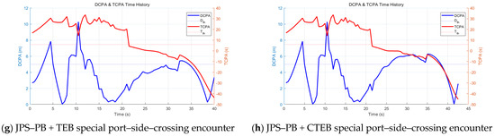
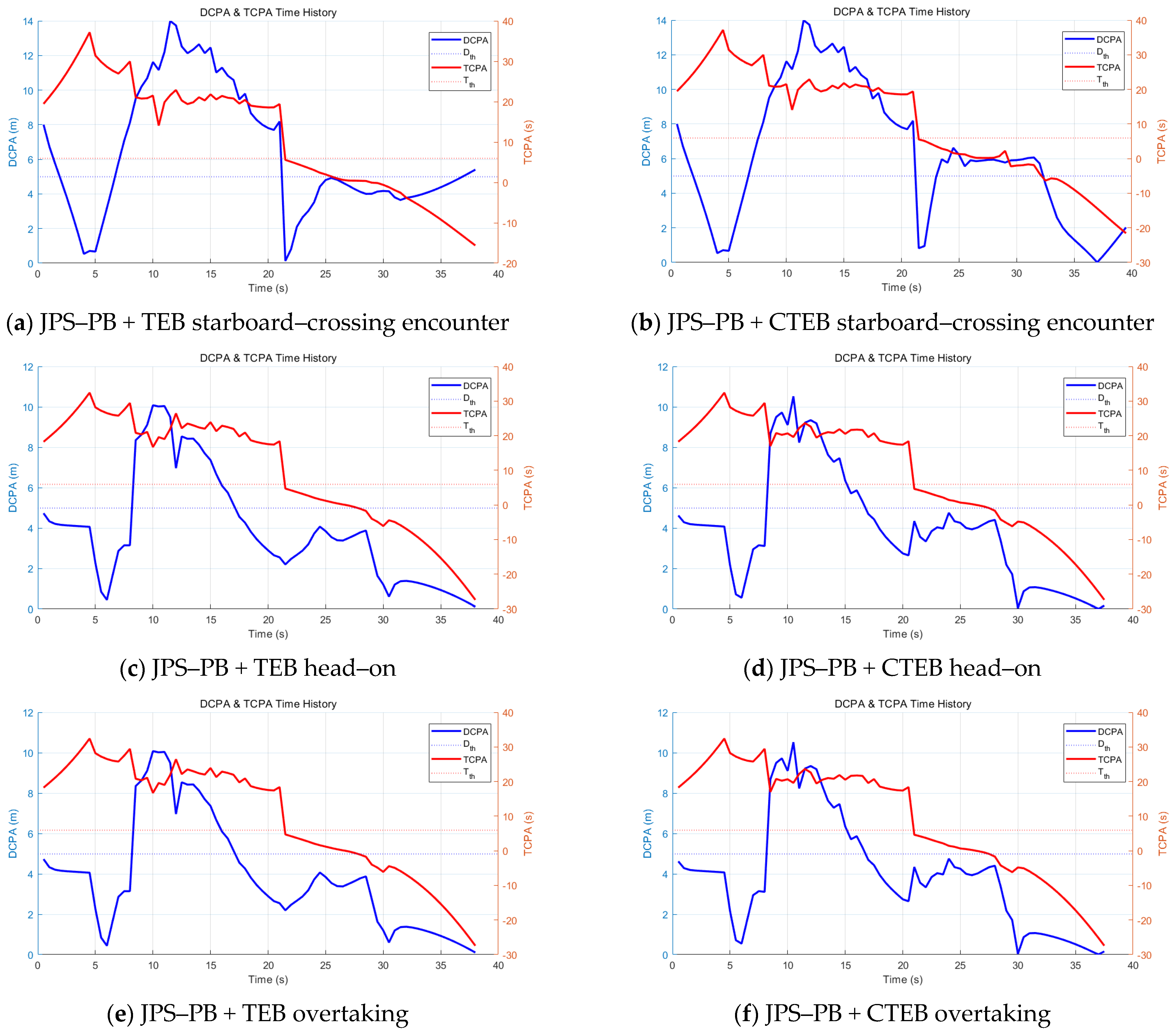
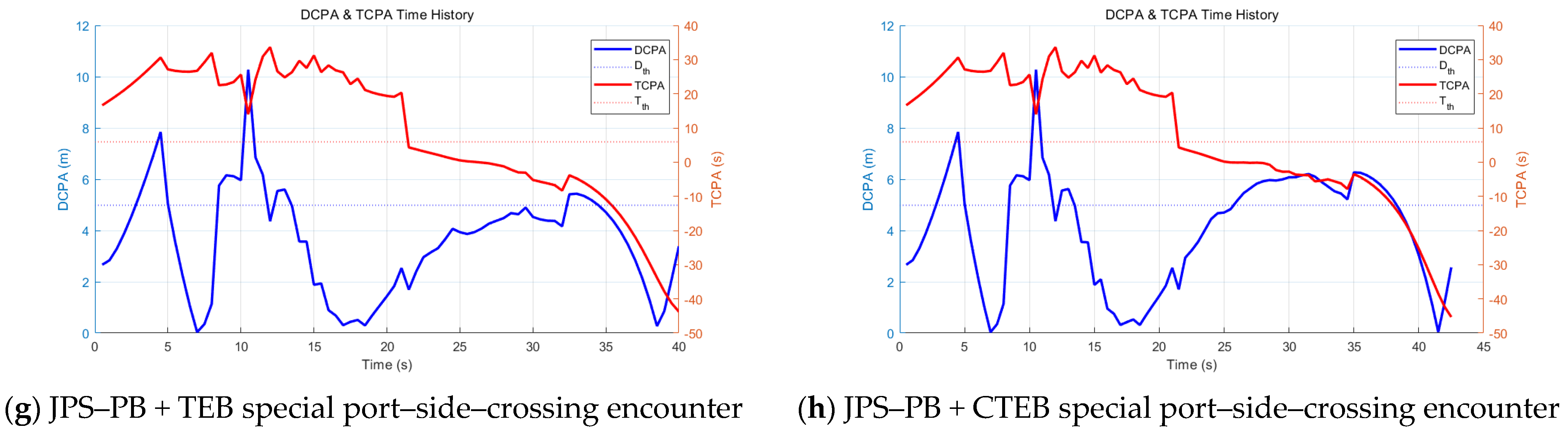
To quantitatively evaluate the collision–avoidance performance of the proposed CTEB algorithm and the conventional TEB algorithm, the DCPA and TCPA are adopted as collision–risk indicators. The corresponding quantitative results are presented in Figure 10.

As shown in

Table 4. DCPA comparison of trajectories generated by JPS–PB integrated with TEB and CTEB.

Algorithm	Starboard–Crossing Encounter	Encounter	Overtaking	Special Port–Side–Crossing Encounter
JPS–PB + traditional TEB	0.128	2.194	1.071	0.276
JPS–PB + CTEB	0.823	2.644	1.122	0.314

, the proposed CTEB algorithm consistently achieves larger DCPA values than the conventional TEB algorithm across all four representative encounter scenarios, indicating an overall improvement in collision–avoidance safety. The detailed results are discussed as follows.

Starboard–crossing encounter: The DCPA increases from 0.128 m to 0.823 m, corresponding to an improvement of approximately 543%, which represents the most significant enhancement among all scenarios. This substantial improvement can be attributed to the fact that CTEB strictly complies with COLREGs by guiding the own vessel to alter course to starboard and pass astern of the target vessel. In contrast, the conventional TEB algorithm generates a port–side maneuver that cuts across the bow of the target vessel, resulting in a considerably smaller separation distance. Consequently, the minimum encounter distance between the two vessels is significantly increased under the proposed method.

Head–on encounter: The DCPA increases from 2.194 m to 2.644 m, corresponding to an improvement of 20.5%. Since the conventional TEB algorithm also tends to generate a starboard–side avoidance maneuver in this scenario, the performance gain achieved by CTEB is less pronounced than that observed in the starboard–crossing encounter. Nevertheless, the larger DCPA obtained by CTEB demonstrates its ability to maintain a safer separation distance while complying with COLREGs requirements.

Overtaking encounter: The DCPA increases from 1.071 m to 1.122 m, representing an improvement of approximately 4.8%. In this scenario, the target vessel travels in a similar direction and is located on the starboard side of the own vessel. The proposed CTEB algorithm penalizes maneuvers that continue approaching the target vessel from the starboard side, thereby encouraging the own vessel to deviate toward the port side and safely overtake the target vessel. Since both algorithms generate a similar initial port–side avoidance maneuver, the resulting improvement in DCPA is relatively limited.

Special port–side–crossing encounter: The DCPA increases from 0.276 m to 0.314 m, corresponding to an improvement of approximately 13.8%. The relatively modest gain is mainly because the conventional TEB algorithm also produces a qualitatively similar avoidance maneuver in this scenario. However, CTEB explicitly determines whether a stand–on vessel should initiate collision–avoidance action under hazardous circumstances through the proposed risk activation function. As a result, the maneuver generated possesses a clearer regulatory interpretation and stronger consistency with COLREGs.

In summary, by reformulating COLREGs requirements as differentiable cost functions and embedding them into the TEB optimization framework, the proposed CTEB algorithm enables collision–avoidance decisions to simultaneously satisfy regulatory compliance and navigational safety requirements. The improvement is particularly significant in encounter situations where COLREGs specify explicit maneuvering directions, demonstrating the effectiveness of the proposed rule–aware trajectory optimization framework.

4.2. Robustness Analysis of CTEB–Related Parameters

To evaluate the sensitivity of the proposed CTEB algorithm to parameter variations under practical deployment conditions, a starboard–crossing encounter scenario is selected as the benchmark test case. Three key parameters that have the most significant influence on collision–avoidance decision making, namely the danger–distance threshold ${\mathit{D}}_{\mathit{t}\mathit{h}}$, the danger–time threshold ${\mathit{T}}_{\mathit{th}}$, and the COLREGs cost weight ${\gamma }_{col}$, are investigated through a ‘one–factor–at–a–time’ sensitivity analysis.

A controlled–variable approach is adopted in which only one parameter is varied while all remaining parameters are fixed at their baseline values, namely ([${\mathit{D}}_{\mathit{t}\mathit{h}}$, ${\mathit{T}}_{\mathit{th}}$, ${\gamma }_{col}$] = [5 m, 6 s, 10]). The evaluation focuses primarily on two performance indicators: the DCPA and compliance with COLREGs.

(1)

Sensitivity Analysis of the Danger–Distance Threshold ${\mathit{D}}_{\mathit{th}}$

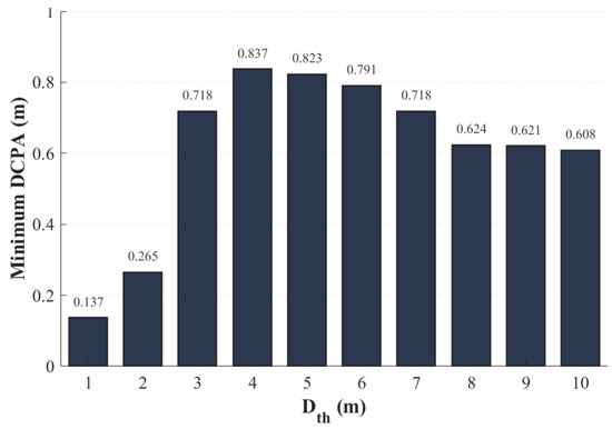
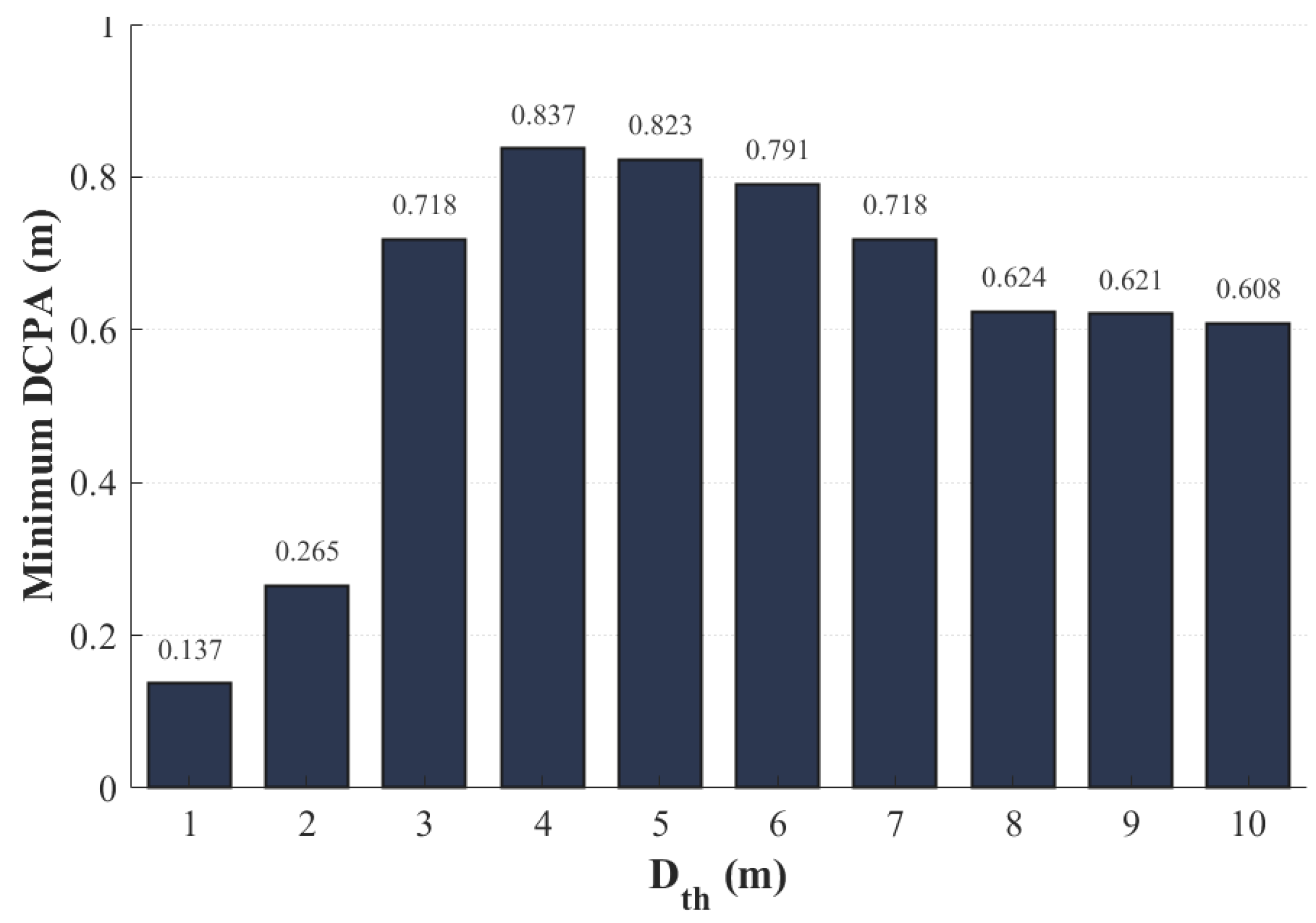
The danger–distance threshold ${\mathit{D}}_{\mathit{t}\mathit{h}}$ is varied from 1 m to 10 m with an increment of 1 m. For each parameter setting, the starboard–crossing encounter scenario described in the previous section is reproduced using the proposed CTEB algorithm. The minimum DCPA obtained under each value of ${\mathit{D}}_{\mathit{t}\mathit{h}}$ is then recorded and compared. The corresponding results are presented in Figure 11.

Analysis of the experimental results indicates that when ${\mathit{D}}_{\mathit{t}\mathit{h}} < 3$, the danger–distance threshold is relatively small, causing the collision–avoidance cost function to be activated only when the own vessel approaches the target vessel at a very close range. Consequently, the resulting DCPA remains small, leading to a relatively high collision risk.

When ${\mathit{D}}_{\mathit{t}\mathit{h}}$∈ [3, 7], the collision–avoidance cost is activated at an appropriate stage of the encounter. This provides the own vessel with sufficient time to perform a smooth starboard avoidance maneuver, resulting in the largest DCPA values observed in the experiment. Therefore, this interval can be regarded as the most suitable range for the danger–distance threshold under the considered navigation scenario.

When ${\mathit{D}}_{\mathit{t}\mathit{h}} > 7$, the collision–avoidance cost is triggered excessively early. As a result, the own vessel begins to alter course while still far from the target vessel. According to the design of the proposed cost function, once the own vessel performs the desired avoidance maneuver, the collision–avoidance cost ${\mathit{f}}_{\mathit{col}}$ decreases accordingly. Meanwhile, the continuous attraction of the global reference path gradually drives the vessel back toward the planned route. This corrective behavior partially offsets the early avoidance maneuver and ultimately leads to a reduction in DCPA.

(2)

Sensitivity Analysis of the Danger–Time Threshold ${\mathit{T}}_{\mathit{th}}$

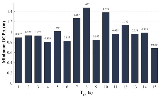
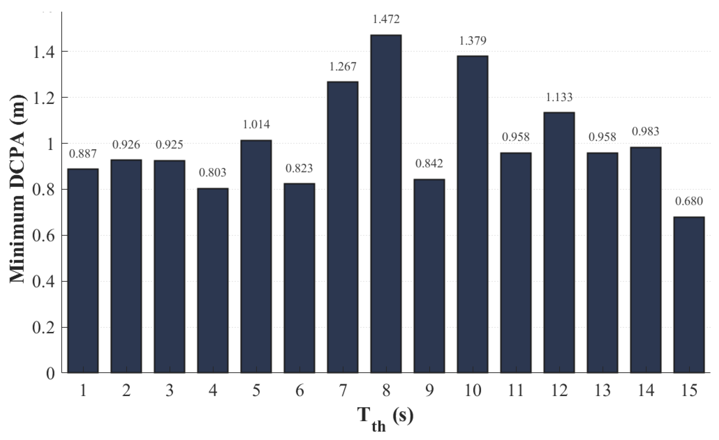
To investigate the influence of the danger–time threshold on collision–avoidance performance, ${\mathit{T}}_{\mathit{t}\mathit{h}}$ is varied from 1 s to 15 s with an increment of 1 s. For each parameter setting, the starboard–crossing encounter scenario described in the previous section is reproduced using the proposed CTEB algorithm. The minimum DCPA obtained under each value of ${\mathit{T}}_{\mathit{t}\mathit{h}}$ is recorded and compared. The corresponding results are shown in Figure 12.

During the receding–horizon optimization process of CTEB, each adjustment of the own–ship heading angle β modifies the relative–motion vector between the two vessels, which in turn alters the instantaneous estimate of the TCPA. Consequently, the response of the danger–time threshold ${\mathit{T}}_{\mathit{t}\mathit{h}}$ exhibits a pronounced multi–peak characteristic rather than a monotonic trend.

The experimental results indicate that when ${\mathit{T}}_{\mathit{t}\mathit{h}}$∈ [1, 6], the average DCPA is 0.896 m with a relatively small fluctuation range and a coefficient of variation of 8.3%. This suggests that an excessively short prediction horizon prevents the algorithm from initiating collision–avoidance maneuvers sufficiently early, resulting in stable but suboptimal avoidance performance.

When ${\mathit{T}}_{\mathit{t}\mathit{h}}$∈ [7, 10], the average DCPA increases substantially to 1.240 m, representing an improvement of 38.4% compared with the short–horizon interval. This range contains both the global maximum and secondary peak values of DCPA. Although the coefficient of variation increases to 19.7%, indicating larger fluctuations, the overall collision–avoidance performance is significantly superior. Therefore, this interval can be regarded as the recommended operating range for the danger–time threshold.

When ${\mathit{T}}_{\mathit{t}\mathit{h}}$∈ [11, 15], the average DCPA decreases to 0.942 m, corresponding to a reduction of 31.6% relative to the recommended interval. Furthermore, the global minimum DCPA is observed within this range. This phenomenon indicates that an excessively long prediction horizon causes the collision–avoidance cost to remain active for an extended period. Under the continuous influence of the global–path tracking objective, the own vessel repeatedly adjusts its heading during navigation, thereby weakening the effectiveness of the avoidance maneuver and reducing the final separation distance.

(3)

Sensitivity Analysis of the COLREGs Cost Weight ${\gamma }_{col}$

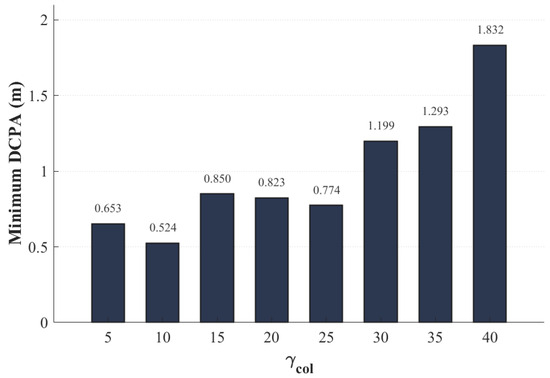
To investigate the influence of the COLREGs cost weight on collision–avoidance performance, ${\gamma }_{col}$ is varied from 5 to 40 with an increment of 5. For each parameter setting, the starboard–crossing encounter scenario described previously is reproduced using the proposed CTEB algorithm. The minimum DCPA obtained under each value of ${\gamma }_{col}$ is recorded and compared. The corresponding results are presented in Figure 13.

The experimental results indicate that the COLREGs cost weight has a significant influence on the collision–avoidance behavior of the proposed CTEB algorithm. When ${\gamma }_{col}$ is small, the contribution of the COLREGs constraint to the overall objective function is relatively weak. In this case, its influence is diluted by competing terms such as path–tracking cost, time–optimal cost, and trajectory–smoothing cost. Although the own vessel is still able to avoid obstacles, the degree of compliance with COLREGs is insufficient, and the avoidance maneuvers remain relatively conservative, resulting in generally small DCPA values.

As ${\gamma }_{col}$ increases, the guiding effect of the COLREGs constraint on trajectory optimization becomes progressively stronger. The own vessel is more inclined to follow COLREGs–compliant maneuvers, actively turning to starboard and passing astern of the target vessel, thereby effectively increasing the minimum separation distance between the two vessels. Although fluctuations are observed when ${\gamma }_{col}$ = 10, the overall trend remains increasing. This behavior is primarily attributed to the receding–horizon nature of the TEB optimization framework. Under different weight configurations, the competition among rule–based cost, path–tracking cost, and obstacle–avoidance cost leads to variations in locally optimal solutions.

In summary, the proposed CTEB algorithm demonstrates good robustness with respect to variations in the COLREGs cost weight. Within a relatively wide parameter range, the algorithm consistently maintains COLREGs–compliant collision–avoidance behavior.

5. Conclusions

5.1. Main Achievements

To address the issues of global path redundancy, discontinuous path turning, and the lack of explicit COLREGs compliance in local dynamic obstacle avoidance for ASVs operating in complex maritime environments, this study proposed an intelligent path–planning framework integrating the JPS–PB algorithm and the CTEB algorithm. The effectiveness of the proposed method was validated through global path–planning experiments, representative encounter–scenario simulations, and parameter sensitivity analyses.

For global path planning, a JPS–PB algorithm was developed by incorporating redundant–node elimination and cubic Bezier curve smoothing into the conventional JPS framework. The ablation study demonstrated that redundant–node elimination primarily contributes to path–length reduction and cumulative steering–angle minimization, whereas Bezier curve smoothing is mainly responsible for reducing the maximum steering angle and improving path continuity. Compared with the conventional JPS algorithm, the proposed JPS–PB method effectively eliminates redundant path segments and sharp turning points, generating shorter and smoother reference paths that better satisfy ASV kinematic constraints. Furthermore, compared with recently reported JPS–based improvements, JPS–PB achieves a favorable balance among path length, cumulative steering angle, and computational efficiency, providing high–quality global guidance for subsequent local trajectory optimization.

For local dynamic obstacle avoidance, typical encounter rules defined in the International Regulations for Preventing Collisions at Sea (COLREGs), including head–on, crossing, and overtaking situations, were reformulated as differentiable cost functions and incorporated into the TEB optimization framework together with the DCPA, TCPA, and a risk activation mechanism. The resulting CTEB algorithm enables explicit consideration of maritime navigation rules during trajectory optimization. Simulation results showed that CTEB consistently achieved larger DCPA values than the conventional TEB algorithm in starboard–crossing encounter, head–on, overtaking, and special port–side–crossing encounter scenarios. In addition, the generated avoidance maneuvers exhibited improved compliance with COLREGs requirements. These results demonstrate that the proposed method effectively compensates for the lack of explicit maritime–rule constraints in conventional TEB and enhances both navigational safety and regulatory compliance during dynamic obstacle avoidance.

For the integrated planning framework, the global reference path generated by JPS–PB was employed as guidance for local planning, while CTEB was activated whenever potential collision risks with dynamic vessels were detected. The resulting hybrid architecture successfully combines high–quality global path generation with rule–compliant local collision avoidance, enabling smooth and safe navigation in dynamic maritime environments. Moreover, parameter sensitivity analyses demonstrated that the proposed CTEB algorithm maintains stable collision–avoidance performance under variations in the danger–distance threshold, danger–time threshold, and COLREGs cost weight. These results further demonstrate the robustness and practical applicability of the proposed framework and highlight its potential for practical deployment in autonomous ASV navigation systems. It should be noted, however, that the validation of the proposed framework is primarily based on simulation using a simplified 3–DOF vessel model and representative encounter scenarios. Future work will include more complex multi–vessel scenarios and experimental or sea–trial validation.

5.2. Future Work

The 3–DOF kinematic model employed in this study adequately captures the planar position, heading, and relative motion between the own vessel and the target vessels. However, it does not account for propulsion system dynamics, rudder response characteristics, or environmental disturbances such as wind, waves, and currents, all of which can significantly influence trajectory tracking and control performance in real operations. To bridge this gap, future work will introduce a higher–fidelity ship dynamics model and incorporate environmental disturbance modeling to systematically investigate the trackability and control robustness of the planned trajectories, thereby enhancing the practical applicability of the proposed algorithm in realistic marine environments.

Regarding the global planning module, the performance validation of the JPS–PB algorithm in this paper was primarily conducted on a limited set of grid maps with typical start–goal configurations. In subsequent studies, we will construct a multi–scale map test suite covering various map sizes, obstacle densities, and complexity levels, and perform large–scale statistical experiments with multiple random start and goal pairs. This will allow a comprehensive evaluation of the algorithm from multiple perspectives—including path length, planning time, number of expanded nodes, and path smoothness—to further substantiate its generality and stability in complex maritime environments.

For the local planning component, the validation of the CTEB algorithm has mainly focused on representative encounter scenarios, including starboard–crossing encounters, head–on, overtaking, and the special case of the port–side–crossing encounters. More challenging conditions—such as dense traffic, multiple dynamic obstacles, sequential encounters, and confined waterways—have not yet been sufficiently explored. To address this, future work will design simulation scenarios involving multi–vessel cooperative encounters, congested waterway navigation, and complex dynamic environments, so as to thoroughly assess the robustness and COLREGs compliance of the algorithm under demanding conditions. Moreover, the current comparative baselines are mostly limited to the traditional TEB and a few similar global planning algorithms. In future research, we will broaden the comparison to include state–of–the–art COLREGs–compliant methods based on velocity obstacles, dynamic window approach, model predictive control, and reinforcement learning. This extended benchmarking will be carried out in terms of collision–avoidance safety, rule compliance, computational efficiency, and trajectory quality, enabling a more comprehensive assessment of the strengths and limitations of our method relative to current mainstream autonomous maritime collision–avoidance techniques.

Finally, it should be noted that all validations in this work have been performed in simulation environments; hardware–in–the–loop testing and field experiments on real ASV platforms have not yet been conducted. To advance the proposed method toward practical engineering deployment, we plan to carry out semi–physical simulations and real–vessel trials using ROS/Gazebo, digital twin marine environments, and actual ASV platforms. These experiments will evaluate the algorithm’s performance under realistic disturbances such as sensor noise, communication delays, and model inaccuracies, thereby facilitating the transition of our approach from theoretical development to operational autonomous navigation at sea.

References

- Namgung, H.; Kim, J.S.; Jang, D. Path planning and collision avoidance technologies for maritime autonomous surface ships: A review of COLREGs compliance, algorithmic trends and the Navigation-GPT framework. J. Navig. 2025, 78, 430–450. [Google Scholar] [CrossRef] [Scilit]
- Tang, Y.; Zakaria, M.A.; Younas, M. Path Planning Trends for Autonomous Mobile Robot Navigation: A Review. Sensors 2025, 25, 1206. [Google Scholar] [CrossRef] [Scilit] [PubMed]
- Harabor, D.; Grastien, A. Online graph pruning for pathfinding on grid maps. In Proceedings of the AAAI Conference on Artificial Intelligence, San Francisco, CA, USA, 7–11 August 2011; pp. 1114–1119. [Google Scholar] [CrossRef] [Scilit]
- An, Z.; Li, C.; Han, Y.; Niu, M. Improved Bidirectional JPS Algorithm for Mobile Robot Path Planning in Complex Environments. Comput. Mater. Contin. 2025, 83, 1347–1366. [Google Scholar] [CrossRef] [Scilit]
- Wang, F.; Sun, W.; Yan, P.; Wei, H.; Lu, H. Research on Path Planning for Robots with Improved A* Algorithm under Bidirectional JPS Strategy. Appl. Sci. 2024, 14, 5622. [Google Scholar] [CrossRef] [Scilit]
- Liu, R.; Wang, X.; Wu, D.; Xie, C. Improved Bidirectional Dynamic JPS Algorithm for Global Path Planning. In Lecture Notes in Electrical Engineering; Springer: Heidelberg, Germany, 2023. [Google Scholar] [CrossRef] [Scilit]
- Yin, X.; Dong, W.; Wang, X.; Yu, Y.; Yao, D. Route planning of mobile robot based on improved RRT star and TEB algorithm. Sci. Rep. 2024, 14, 8942. [Google Scholar] [CrossRef] [Scilit] [PubMed]
- Shi, Y.; Huang, S.; Li, M. An Improved Global and Local Fusion Path-Planning Algorithm for Mobile Robots. Sensors 2024, 24, 7950. [Google Scholar] [CrossRef] [Scilit] [PubMed]
- Rösmann, C.; Feiten, W.; Wösch, T.; Hoffmann, F.; Bertram, T. Integrated online trajectory planning and optimization in distinctive topologies. Robot. Auton. Syst. 2017, 88, 142–153. [Google Scholar] [CrossRef] [Scilit]
- Chen, L.; Liu, R.; Jia, D.; Xian, S.; Ma, G. Improvement of the TEB Algorithm for Local Path Planning of Car-like Mobile Robots Based on Fuzzy Logic Control. Actuators 2025, 14, 12. [Google Scholar] [CrossRef] [Scilit]
- Kulathunga, G.; Yilmaz, A.; Huang, Z.; Hroob, I.; Arunachalam, H.; Guevara, L.; Klimchik, A.; Cielniak, G.; Hanheide, M. Resilient Timed Elastic Band Planner for Collision-Free Navigation in Unknown Environments. J. Field Robot. 2025, 42, 3902–3917. [Google Scholar] [CrossRef] [Scilit]
- Xu, D.H.; Yang, J.; Zhou, X.Q.; Xu, H. Hybrid path planning method for USV using bidirectional A* and improved DWA considering the manoeuvrability and COLREGs. Ocean Eng. 2024, 298, 117210. [Google Scholar] [CrossRef] [Scilit]
- Liu, S.; Wang, X.; Wu, Y.; Li, Q.; Yan, J.; Levin, E. Path planning method for USVs based on improved DWA and COLREGs. Intell. Robot. 2024, 4, 385–405. [Google Scholar] [CrossRef] [Scilit]
- Li, J.; Liu, Y.; Yuan, W.; Li, Z. Hybrid Path Planning Strategy Based on Improved Particle Swarm Optimisation Algorithm Combined with DWA for Unmanned Surface Vehicles. J. Mar. Sci. Eng. 2024, 12, 1268. [Google Scholar] [CrossRef] [Scilit]
- Liu, Y.; Sun, Z.; Wan, J.; Li, H.; Yang, D.; Li, Y.; Fu, W.; Yu, Z.; Sun, J. Hybrid Path Planning Method for USV Based on Improved A-Star and Dynamic Window Approach. J. Mar. Sci. Eng. 2025, 13, 934. [Google Scholar] [CrossRef] [Scilit]
- Potočnik, P. Model Predictive Control for Autonomous Ship Navigation with COLREG-Compliant Collision Avoidance. J. Mar. Sci. Eng. 2025, 13, 1246. [Google Scholar] [CrossRef] [Scilit]
- Gleeson, J.; Dunbabin, M.; Ford, J.J. Addressing COLREG Rule 2b: COLREG and Risk Aware Manoeuvre-Based Predictive Planning. IEEE Robot. Autom. Lett. 2025, 10, 7310–7317. [Google Scholar] [CrossRef] [Scilit]
- Wen, N.; Long, Y.; Zhang, R.; Liu, G.; Wan, W.; Jiao, D. COLREGs-Based Path Planning for USVs Using the Deep Reinforcement Learning Strategy. J. Mar. Sci. Eng. 2023, 11, 2334. [Google Scholar] [CrossRef] [Scilit]
- Sonntag, V.; Perrusquía, A.; Tsourdos, A.; Guo, W. A COLREGs compliance reinforcement learning approach for USV manoeuvring in track-following and collision avoidance problems. Ocean Eng. 2025, 316, 119907. [Google Scholar] [CrossRef] [Scilit]
- Pan, R.; Zhang, W.; Wang, S.; Kang, S. Deep reinforcement learning model for multi-ship collision avoidance decision making: Design, implementation and performance analysis. Sci. Rep. 2025, 15, 21250. [Google Scholar] [CrossRef] [Scilit] [PubMed]
- Kümmerle, R.; Grisetti, G.; Strasdat, H.; Konolige, K.; Burgard, W. G2o: A general framework for graph optimization. In Proceedings of the 2011 IEEE International Conference on Robotics and Automation; IEEE: Shanghai, China, 2011; pp. 3607–3613. [Google Scholar] [CrossRef] [Scilit]
- Woo, J.; Kim, N. Vision-based target motion analysis and collision avoidance of unmanned surface vehicles. Proc. Inst. Mech. Eng. Part M J. Eng. Marit. Environ. 2016, 230, 566–578. [Google Scholar] [CrossRef] [Scilit]
Disclaimer/Publisher’s Note: The statements, opinions and data contained in all publications are solely those of the individual author(s) and contributor(s) and not of MDPI and/or the editor(s). MDPI and/or the editor(s) disclaim responsibility for any injury to people or property resulting from any ideas, methods, instructions or products referred to in the content. |
© 2026 by the authors. Licensee MDPI, Basel, Switzerland. This article is an open access article distributed under the terms and conditions of the Creative Commons Attribution (CC BY) license.