


Abstract
Langmuir turbulence is a key and common process in the ocean surface boundary layer, playing a major role in vertical mixing, heat flux, and material transport. However, because direct simulation of Langmuir turbulence demands considerable computational resources, parameterizations within established schemes like the K-profile parameterization (KPP) offer a practical alternative for representing its effects in ocean and climate models. However, Langmuir turbulence parameterizations based on KPP may overestimate vertical mixing when convection is significant. To address this, we introduce a dynamic weighting factor, based on characteristic velocity scales, to balance the contributions of convective and Langmuir turbulence. The improved scheme shows a significant enhancement in performance, especially under strong convective conditions. We compare and evaluate the new parameterization schemes against other widely used schemes in three typical scenarios. Additionally, we validate it using large-eddy simulation results and field observation data. Our enhanced mixing scheme is highly competitive and performs robustly under a variety of conditions.
1. Introduction
Langmuir turbulence is a unique turbulent phenomenon in the ocean surface boundary layer, driven by the interaction between waves and currents [1,2,3]. Its primary characteristic is the formation of paired, counter-rotating vortices aligned with the wind direction [4,5]. Langmuir turbulence plays a crucial role in vertical mixing and material transport within the ocean surface layer, significantly affecting the transport of heat, gases, and biogeochemical substances [3,6,7,8,9,10]. The horizontal scale of Langmuir turbulence typically ranges from 10 to 100 m, with lifetimes ranging from several minutes to hours [5]. Due to its complexity, direct simulation of Langmuir turbulence requires extremely high resolution, which remains a challenge due to current computational limitations [11,12]. Therefore, it is essential to develop a parameterization scheme for Langmuir turbulence that balances physical accuracy, numerical efficiency, and stability [13,14].
The development of the Langmuir turbulence parameterization schemes is mainly achieved by improving classical turbulent mixing frameworks, such as the K-profile parameterization (KPP). KPP represents the mixing process by describing the vertical profile of the turbulent diffusion coefficient, with the boundary layer depth determined by a bulk Richardson number criterion [15]. As one of the most widely used boundary layer schemes, KPP serves as the fundamental framework for characterizing upper ocean mixing processes in many ocean circulation and climate models.
The Langmuir turbulence parameterization scheme based on the KPP framework is called KPPLT, where “LT” stands for Langmuir turbulence. The turbulent Langmuir number () is a key parameter in KPPLT. Originally defined by McWilliams et al. (1997), it is given by the following equation [2]:
Here, and are the surface friction velocity and surface Stokes drift velocity, respectively. Subsequent studies have proposed several variants of this turbulent Langmuir number [16,17]. For example, Harcourt and D’Asaro (2008) introduced the surface-layer Langmuir number (), which accounts for the attenuation of Stokes drift with depth [18]. Van Roekel et al. (2012) later developed the surface-layer projected Langmuir number () to account for the effect of wind–wave directional misalignment on Langmuir turbulence [19]:
where and are the surface Stokes drift (averaged over the top 20% of the boundary layer) and the reference Stokes drift at a certain depth in the lower mixed layer, respectively; is the angle between the wave and the wind, and is the angle between the wind and the Langmuir circulation [18,19].
Based on the turbulent Langmuir number and its variants, several Langmuir enhancement factors have been proposed. These factors aim to enhance the vertical mixing coefficient in KPPLT by increasing turbulent velocity. However, their performance is highly sensitive to real ocean conditions, especially under strong convective forcing driven by surface cooling.
For example, McWilliams and Sullivan (2000) proposed a Langmuir enhancement factor , but the power-law relationship of overestimates the strength of Langmuir mixing under strong convective conditions [13,20]. Van Roekel et al. (2012) derived a Langmuir enhancement factor using the surface-layer-projected Langmuir number by fitting against large-eddy simulation (LES) results [19]:
Recently, Wang et al. (2025) proposed an enhancement factor using the turbulent Langmuir number (Equation (1)) and the wave–wind misalignment angle [14]:
The use of as a power-law relationship is physically well-founded: it links the enhancement of turbulent velocity to the characteristic velocity of Langmuir turbulence, [21,22], through the scaling relation [14]. In addition, the wave–wind angle accounts for the effect of wind-wave misalignment on the intensity of Langmuir turbulence.
The enhancement factor in Equation (4) performs well in a modified KPP that uses an integral criterion to determine the boundary layer depth. However, its behavior within the traditional KPP framework—which relies on a bulk Richardson number and remains the standard in many ocean models—has not been thoroughly tested. This lack of evaluation is especially problematic under convective conditions, where the interplay of wind, waves, and surface buoyancy loss complicates boundary layer dynamics. The present study addresses this by systematically assessing and improving the enhancement factor within the traditional KPP framework for convective scenarios.
The rest of this study is organized as follows. Section 2 presents the Langmuir turbulence parameterization scheme based on the traditional KPP framework. Section 3 compares the proposed KPPLT scheme with existing mainstream schemes using three typical convective scenarios, and validates the results with large-eddy simulation (LES) data and field observations. Finally, Section 4 summarizes the main findings and discusses their potential applications and significance.
2. Description of Langmuir Turbulence Parameterization
In KPP, the vertical diffusion coefficient is expressed as follows:
where is the turbulent velocity scale, is the boundary layer depth, is a non-dimensional shape function expressed as , and is a non-dimensional vertical coordinate (with representing the distance from the sea surface). The subscript “x” can represent either the momentum eddy viscosity or the scalar diffusivity [15].
Following McWilliams and Sullivan (2000), Langmuir turbulence in the KPP framework is parameterized by applying an enhancement factor to the turbulent velocity [13]. In this study, we implement the Langmuir enhancement factor (Equation (4)) within the traditional KPP framework.
Preliminary simulations revealed that this enhancement factor (Equation (4)) causes excessive vertical mixing in the traditional KPP framework under strong convective conditions (Appendix A). This degradation likely occurs because the enhancement factor was originally derived for weak convection. An additional cause may be the discrepancy in the boundary layer depth criterion between the traditional KPP and the modified KPP framework for which the Langmuir enhancement factor was designed. This highlights the need for optimization to handle strong convective forcing in the traditional KPP framework.
To address the issue of excessive mixing enhancement caused by strong convection within the traditional KPP framework, we introduce a weighting factor to reduce the contribution of the Langmuir enhancement factor under convective conditions. This approach is similar to that of Smyth et al. (2002) [23], and is defined as follows:
where n is a tuning parameter, is the friction velocity, and is the convective turbulence velocity. The cubic velocity scales () are physically grounded in the scaling of turbulent kinetic energy (TKE) contributions from each process: corresponds to the TKE generated by convection, while scales with the TKE produced by wind-driven shear.
Here, we define slightly different from the conventional form , where d is the distance from the sea surface and h is the boundary layer depth. This depth-dependent allows the convective velocity scale to grow with distance from the surface, capturing the increasing influence of convection with depth [24,25]. Furthermore, , where is a depth-dependent coefficient. In comparison, Smyth et al. (2002) used a constant coefficient of 0.6 in front of the conventional , serving a similar purpose as in this context [23]. Additionally, we define : under surface cooling, and under surface warming or neutral conditions, in agreement with Large et al. (1994) [15].
The calibration of the exponent in Equation (6) is based on the large-eddy simulation (LES) dataset from Li and Fox-Kemper (2017) [26]. This dataset includes a variety of turbulence states, such as shear-driven, convective, and Langmuir turbulence, under different wind speeds, surface heat fluxes, and wave conditions. By minimizing the root mean square error (RMSE) between the parameterized and LES-derived temperature profiles and mixed layer depths, we obtain the optimal value of .
The turbulent velocity in Equation (5) is then modified as follows:
where κ is the von Kármán constant, is the Monin–Obukhov similarity function defined in Large et al. (1994) [15]. The ranges from 0 to 1, and it decreases as convection becomes stronger; namely, acts as a dynamic switch, enabling the Langmuir mixing scheme to appropriately adapt to varying surface cooling conditions.
Moreover, the boundary layer depth in the traditional KPP is determined by the bulk Richardson number [15], namely,
Here, is the buoyancy, and is the ocean current velocity vector. The buoyancy and velocity denote values at the reference depth. represents the unresolved velocity shear effect. Because of , the is implicitly amplified through the Langmuir-enhanced velocity (Equation (7)). In other words, the Langmuir enhancement factor also enhances and thereby implicitly increases the boundary layer depth.
3. Performance Comparisons of Langmuir Mixing Schemes
The General Ocean Turbulence Model (GOTM), a one-dimensional water column model, is employed to examine the performance of Langmuir mixing schemes. GOTM has been widely used as a general platform for the comparison of different Langmuir mixing schemes [12,14].
Our Langmuir mixing scheme, hereafter the WA scheme, is compared with two alternative schemes; the VR scheme by Van Roekel et al. (2012) [19], and the other is the LF scheme by Li and Fox-Kemper (2017) [26]. The former applies the following Langmuir enhancement factor based on the surface-layer projected Langmuir number (Equation (2b)).
The LF scheme retains the Langmuir enhancement factor from the VR scheme (Equation (3)) and additionally modifies the term in the bulk Richardson number (Equation (8)) by incorporating a Langmuir entrainment flux. The modified in the LF scheme is expressed as [26]:
where is the buoyancy frequency, with as the ratio of buoyancy frequency to that at the entrainment depth, as the scalar turbulent velocity scale, and as the surface layer Langmuir number (Equation (2a)).
All three Langmuir mixing schemes (VR, LF, and WA) are implemented within the KPP framework and are thus referred to as KPPLT-VR, KPPLT-LF, and KPPLT-WA, respectively. Next, we evaluate the performance of the three Langmuir mixing schemes, as well as the KPP scheme (without Langmuir turbulence effects), in three convective scenarios: LES with idealized forcing (Section 3.1), LES with realistic forcing (Section 3.2), and field observations (Section 3.3).
3.1. LES with Idealized Forcing
Li and Fox-Kemper (2017) generated an LES dataset of Langmuir turbulence under idealized wind stress, surface heat flux, and wind-aligned Stokes drift [26]. The model domain measured 320 m × 320 m × 163.84 m in the (x, y, z) directions, with horizontal and vertical resolutions of 1.25 m and 0.64 m, respectively. The initial mixed layer depth (MLD) was set at 42 m, with a stratification of applied beneath it. The Coriolis parameter was set to , representing typical mid-latitude conditions.
Eight cases were selected from the LES dataset to evaluate different Langmuir mixing schemes (Table 1). For all cases, wind stress was fixed at 0.144 N/m2, with variations in surface cooling, Langmuir number, and Stokes drift. Simulations were performed for each case using the GOTM model, with a time step of 60 s and a vertical resolution of 0.64 m. The surface cooling exhibits a progressive intensification from weak (Cases 1–2) to strong (Cases 7–8).
Table 1.
Key parameters for each case: the surface heat flux (Q), the surface Stokes drift (us), the turbulent Langmuir number (La), and the surface-layer projected Langmuir number (Laslp) averaged over the whole simulation period.
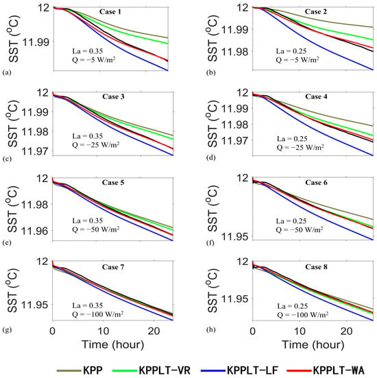
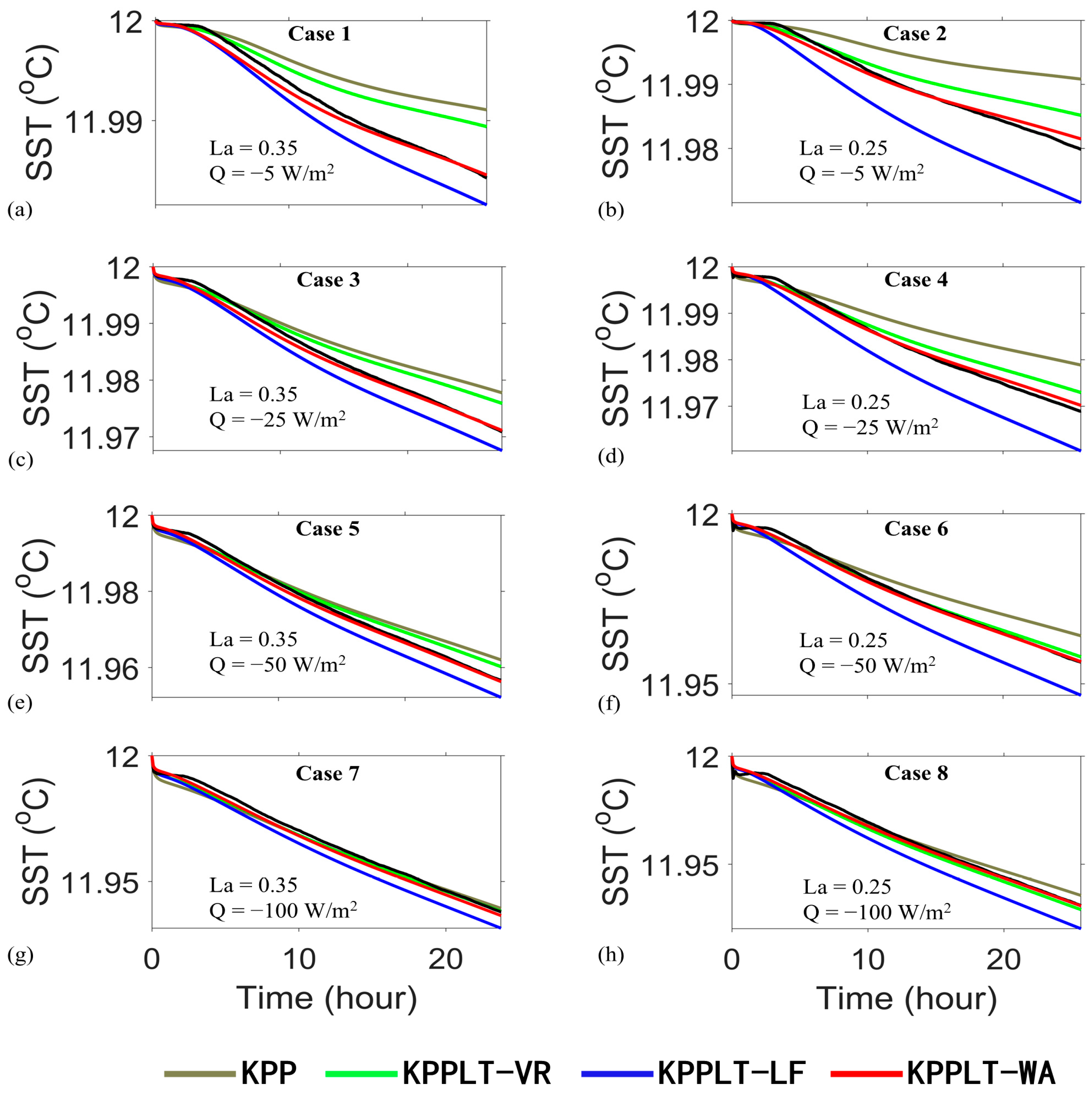
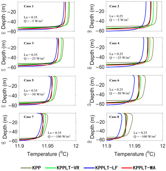
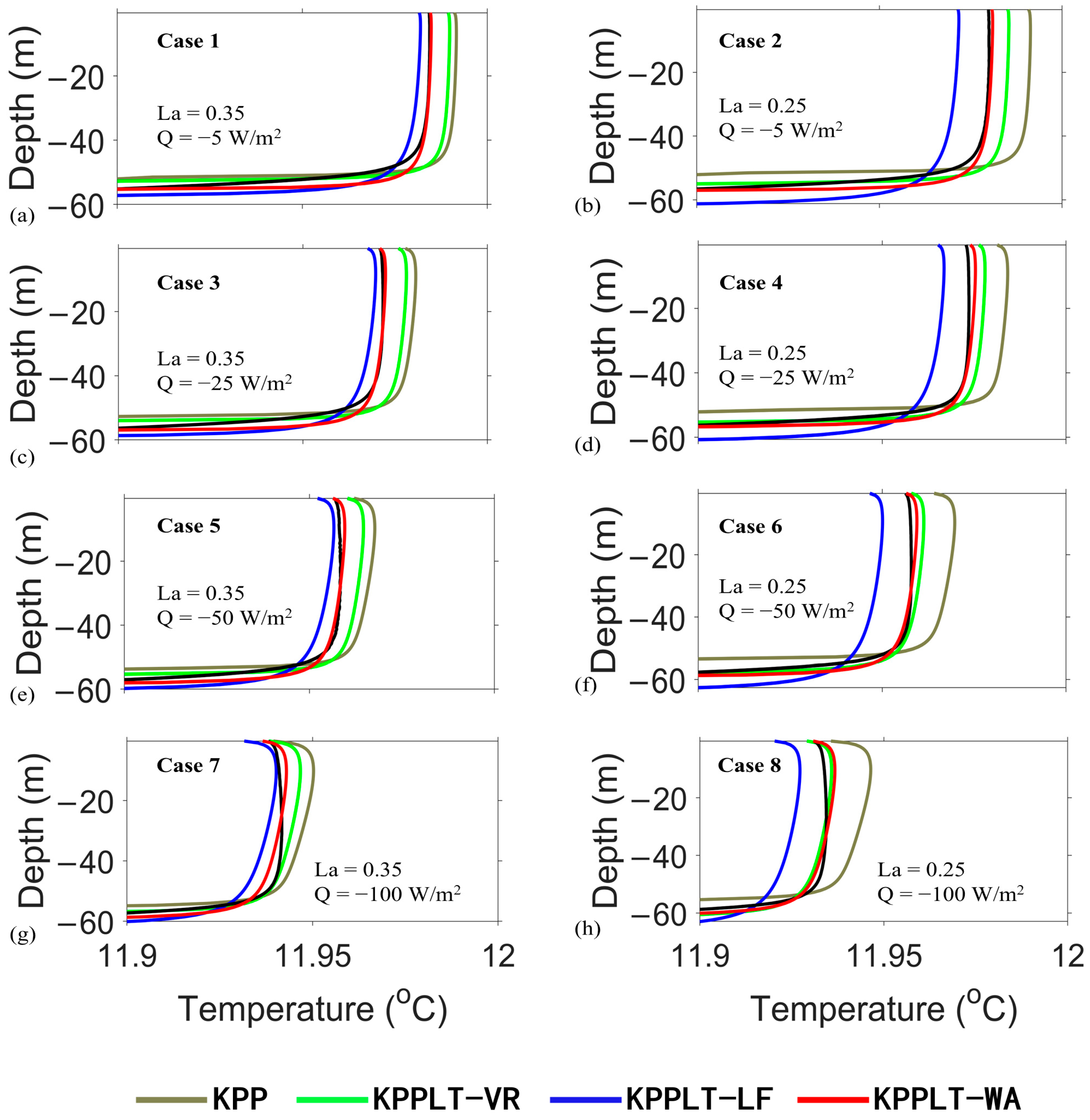
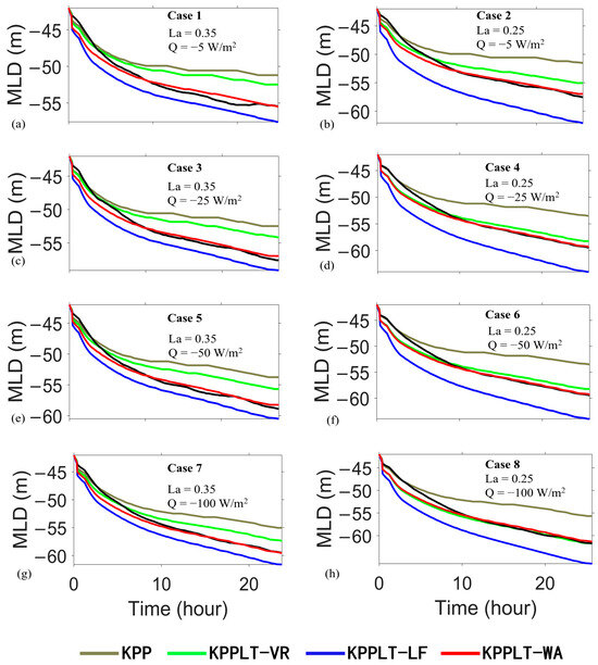
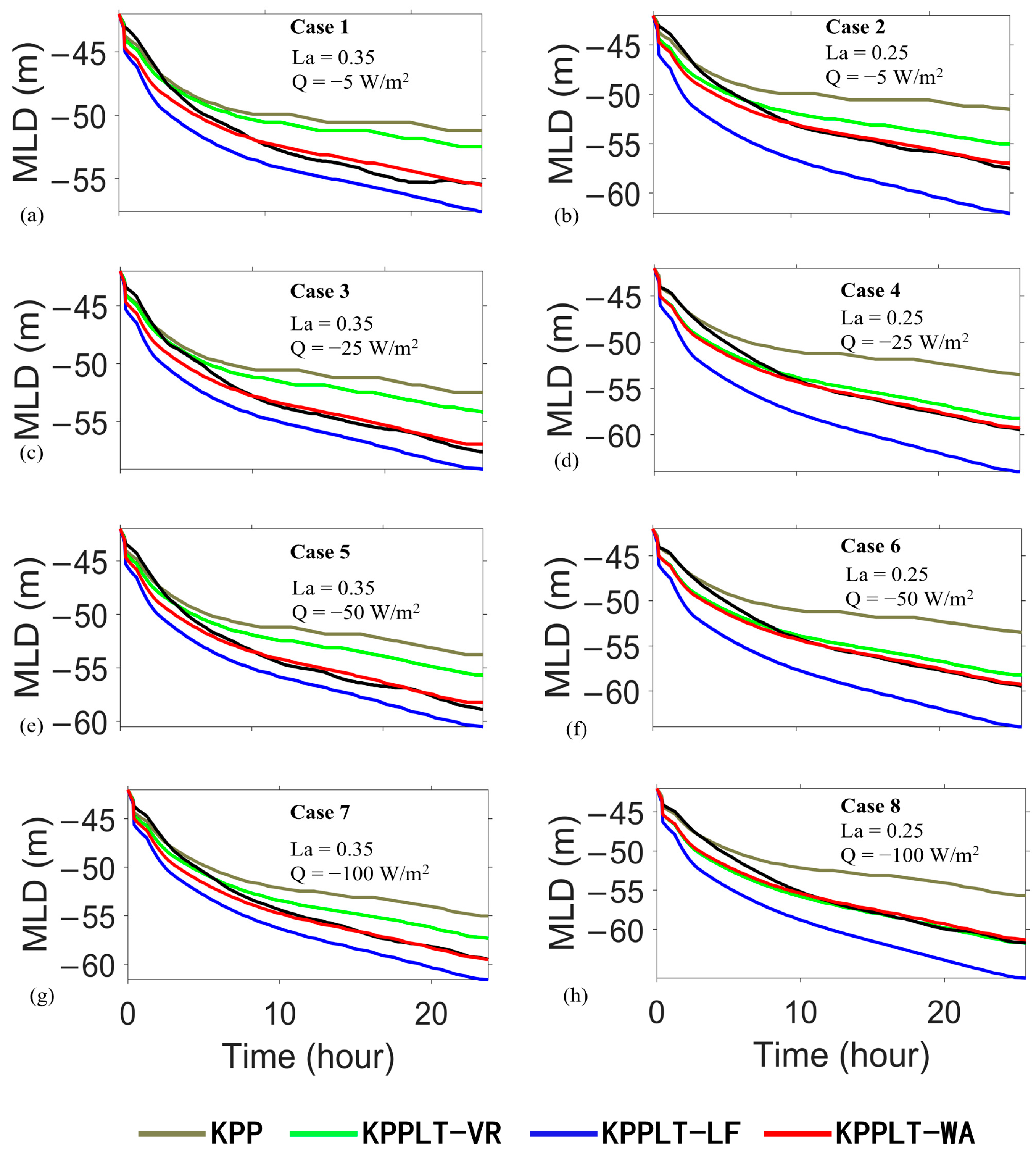
Under the combined effects of surface fluxes and wave forcing, turbulent vertical mixing gradually strengthens over time. This enhanced mixing drives a continuous cooling trend in sea surface temperature (SST, Figure 1), and vertical homogenization of the mixed layer temperature (Figure 2), while promoting a progressive deepening of the mixed layer depth (MLD, Figure 3).
Figure 1.
Sea surface temperature for (a–h) Cases 1–8, respectively. Black lines represent the LES results.
Figure 2.
Temperature profiles at the final time step for (a–h) Cases 1–8, respectively. Black lines represent the LES results.
Figure 3.
Mixed layer depths for (a–h) Cases 1–8, respectively. The MLD corresponds to the depth of maximum buoyancy frequency N2. Black lines represent the LES results.
Under weak surface cooling, all schemes reasonably reproduce mixed-layer temperature homogeneity, with KPPLT-WA achieving the closest agreement with LES results (Figure 2a,b). However, under intense cooling conditions, significant discrepancies in stratification are observed compared with LES outcomes. Particularly, the KPP scheme amplifies vertical thermal heterogeneity, as is theoretically anticipated. The KPP scheme exhibits the weakest vertical mixing characteristics among the four parameterization schemes evaluated. This shortcoming is reflected in a pronounced warm temperature bias in the simulated SST, alongside shallower MLDs compared with LES results.
The KPPLT-VR scheme overall exhibits a warm bias in temperature and a shallow bias in MLD due to its systematic underestimation of Langmuir mixing intensity; namely, the Langmuir enhancement factor of the VR scheme probably underestimates Langmuir mixing. By contrast, a persistent cold bias in temperature and a deep bias in MLD are observed with the KPPLT-LF scheme. This suggests that the incorporation of the Langmuir turbulence-induced entrainment flux (Equation (9)) may cause an overestimation of the boundary layer depth and thus needs further calibration.
Generally, the KPPLT-WA scheme aligns closely with LES across multiple key metrics, particularly in reproducing the temporal evolution of SST, temperature profiles within the mixed layer, and the development of MLD, thus demonstrating superior simulation fidelity.
3.2. LES with Realistic Forcing
An LES dataset of surface boundary-layer turbulence was produced by Yuan et al. (2024) based on observational data from the North Pacific Ocean Station Papa (50.1° N, 144.9° W, Figure 4), including in situ measurements of wind stress, surface waves, shortwave radiation, net heat flux, and temperature–salinity profiles [27]. The model configuration featured a three-dimensional domain measuring 300 m × 300 m × 200 m. The horizontal and near-surface vertical resolutions were 1.875 m and 0.2 m, respectively. All LES cases were initialized using field-measured temperature and salinity data and executed through continuous 10-day simulations, helping to reduce the drift of model results from observations.
Figure 4.
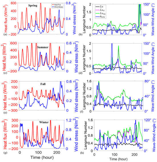
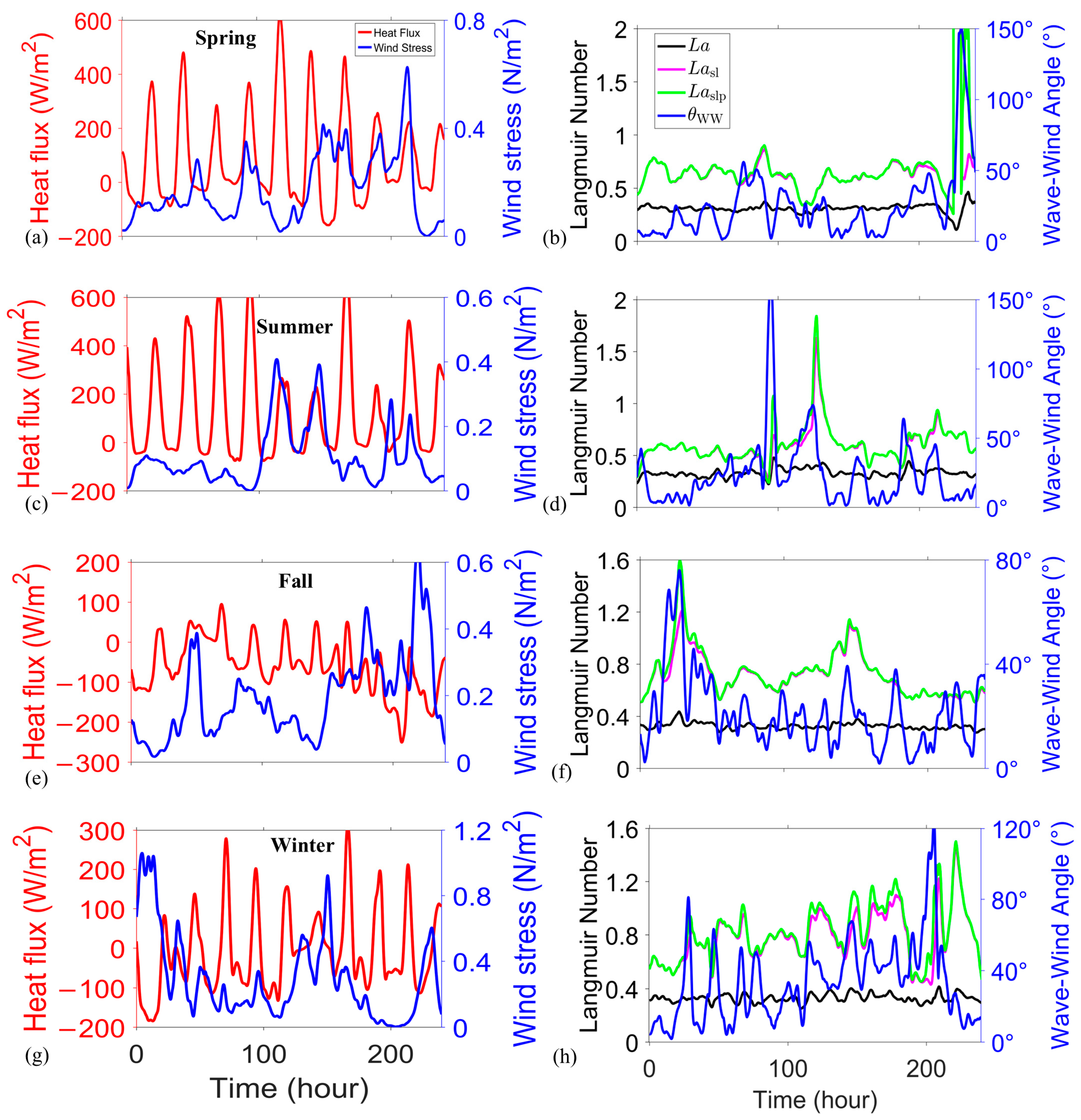
LES with realistic forcing: The left column shows net surface heat flux and wind stress; the right column shows the Langmuir numbers and wind–wave angle. Panels (a,b), (c,d), (e,f), and (g,h) present results for Cases 1, 2, 3, and 4, respectively.
To evaluate the performance and general applicability of Langmuir mixing schemes under realistic conditions, four seasonal cases were chosen to represent typical surface forcing (Figure 4) from the LES dataset: Spring (2 May 2012 to 11 May 2012), Summer (1 June 2012 to 10 June 2012), Fall (8 November 2012 to 17 November 2012), and Winter (26 February 2013 to 7 March 2013). The model configuration employed a time step of 60 s and a vertical resolution of 0.5 m. This setup enabled a seasonal comparative analysis of the performance of different Langmuir mixing schemes in reproducing boundary layer turbulence characteristics.
The turbulent Langmuir number () ranged from 0.2 to 0.5 for these cases, corresponding to significant Langmuir turbulence. The surface-layer Langmuir numbers ( and ) typically fell between 0.3 and 1 (Figure 4).
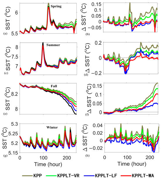
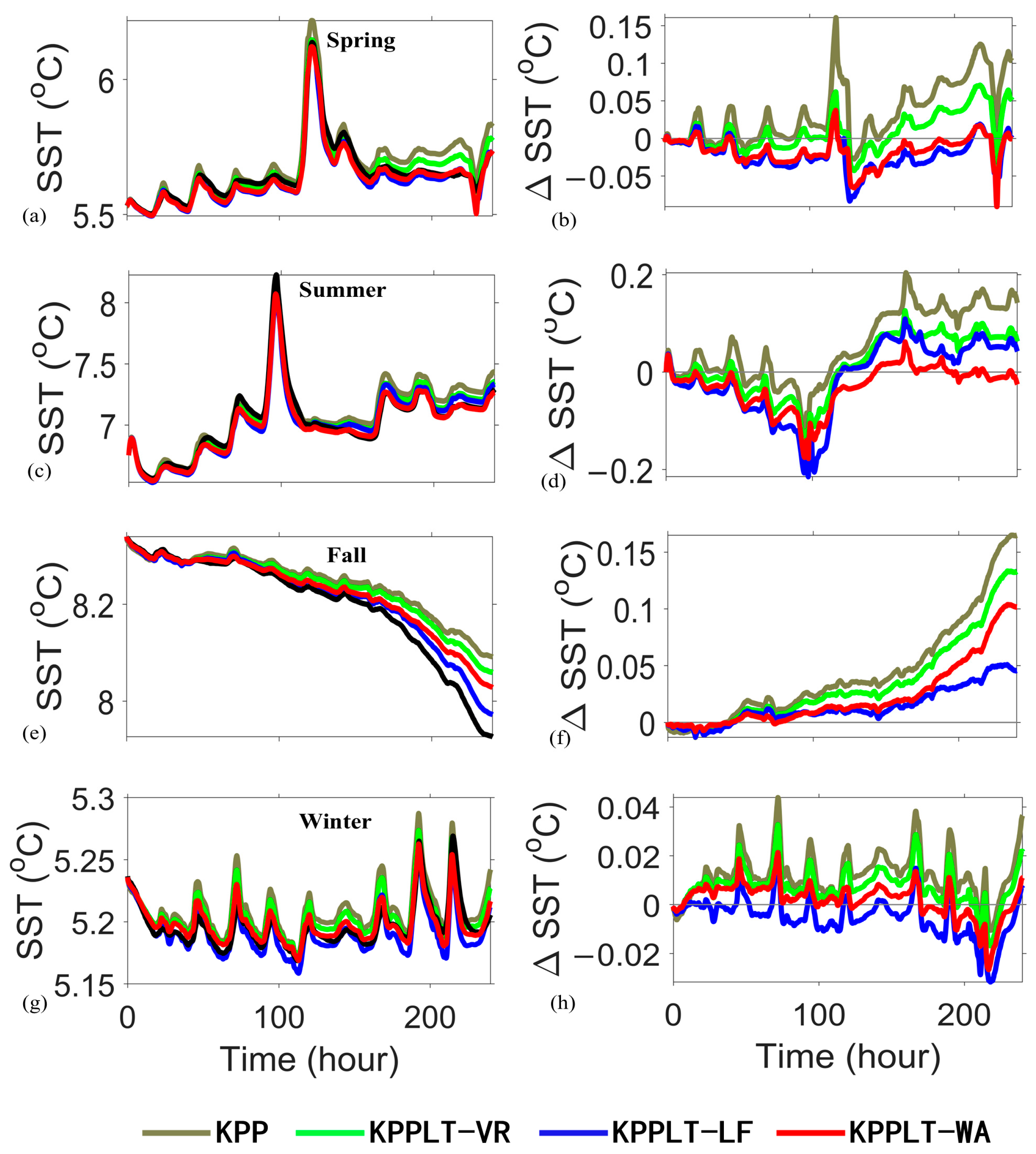
All mixing schemes generally show consistency with LES data in simulating the temporal evolution of SST, successfully capturing its seasonal characteristics (Figure 5). In the spring and summer cases (Figure 5a–d), an overall warming trend is observed, amplifying the deviations between the simulation results and LES data. Notably, the three KPPLT schemes help reduce these deviations relative to the baseline KPP scheme, demonstrating that incorporating Langmuir mixing is critical for improving simulation accuracy.
Figure 5.
LES with realistic forcing: The left column shows sea surface temperature (SST) and the right column shows SST deviations from LES results. Panels (a,b), (c,d), (e,f), and (g,h) present results for Cases 1, 2, 3, and 4, respectively. Black lines represent the LES results.
During the cooling periods in the fall (Figure 5e,f), systematic warm biases are observed across all schemes. Compared with the KPP scheme, the KPPLT-VR scheme yields better results, but it still performs less effectively than both the KPPLT-LF and KPPLT-WA schemes. The simulated temperature shows a slight warm bias, highlighting the limitations of the VR scheme in representing Langmuir mixing effects. In the winter case (Figure 5g,h), under strong cooling conditions, the KPPLT-LF scheme exhibits a cold bias. In contrast, the KPPLT-WA scheme consistently shows smaller temperature biases among all four schemes.
Overall, the KPPLT-WA scheme demonstrates optimal performance in temperature across all four cases. In comparison, the traditional KPP scheme, which fails to account for Langmuir mixing, leads to a warm bias in the SST. The KPPLT-VR scheme shows improvements over the KPP scheme, but the biases remain more pronounced than those of the KPPLT-WA and KPPLT-LF schemes.
3.3. Ocean Station Papa
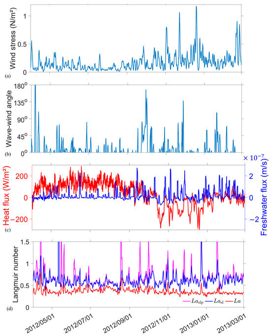
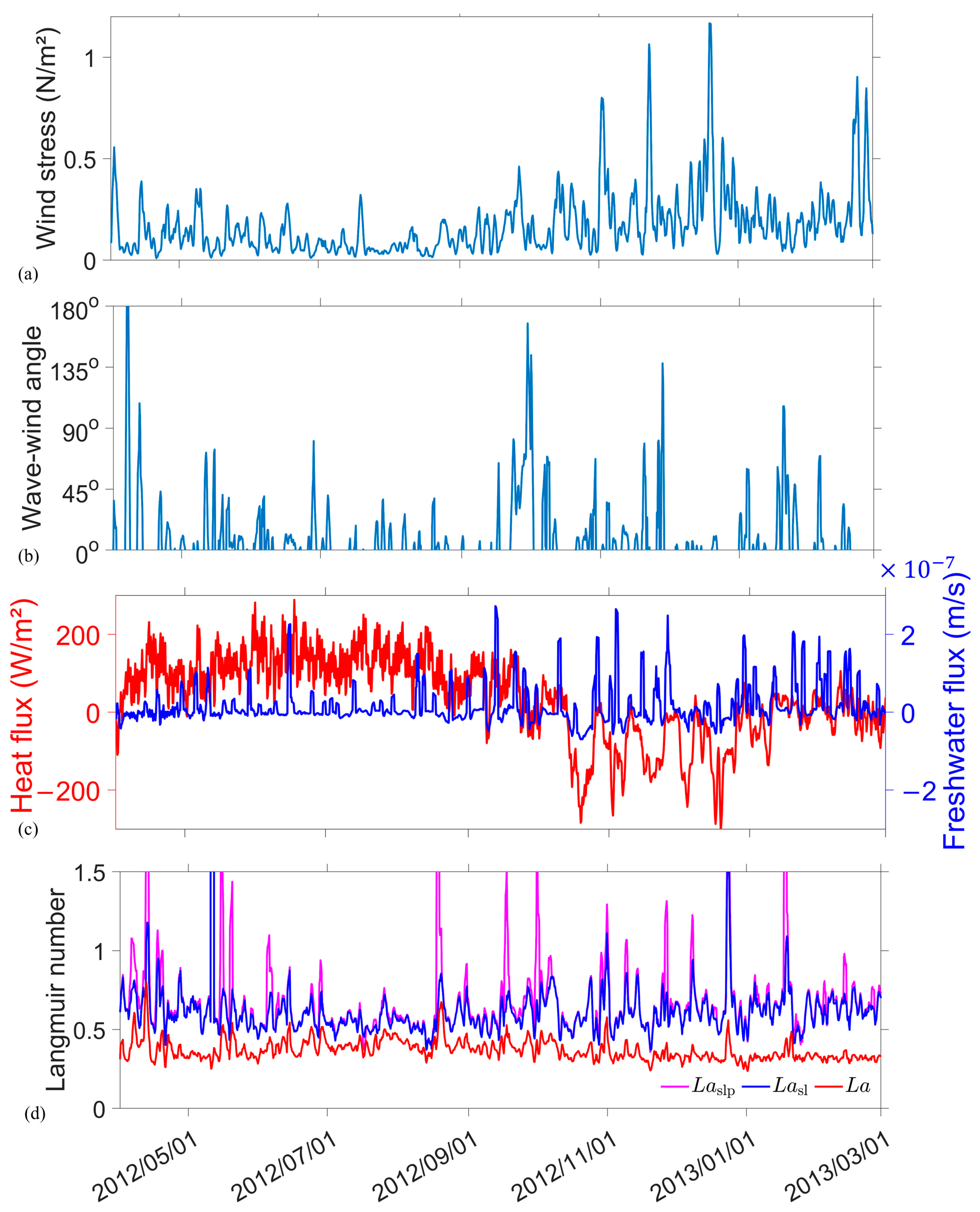
We tested the Langmuir mixing schemes using the long-term meteorological and oceanographic dataset from Ocean Station Papa [12,14]. The study covers the period from 2 April 2012 to 8 March 2013 for the GOTM simulations. In the model setup, the water depth is set to 200 m, and the initial temperature and salinity profiles are taken from mooring measurements. The time step is set to 30 min, and the vertical resolution is 1 m. The simulation begins with a stationary water column, which is then driven by the combined effects of wind stress, freshwater flux, heat flux, and Stokes drift, as shown in Figure 6.
Figure 6.
Ocean Station Papa: (a) wind stress, (b) wave–wind angle, (c) net surface heat flux and freshwater flux, and (d) various Langmuir numbers. A 30 h moving-average filter is applied to all results.
The turbulent Langmuir number () primarily fluctuates between 0.3 and 0.5 during the simulations. In contrast, the surface-layer Langmuir numbers ( and ) show a wider range of fluctuations, approximately between 0.4 and 1.2 (Figure 6d).
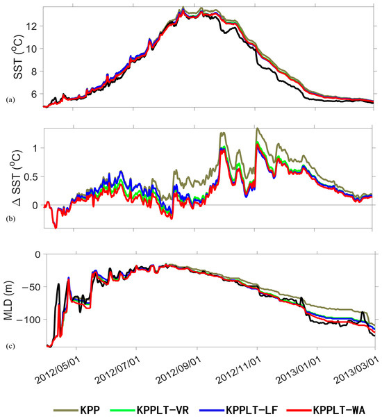
All schemes captured the seasonal variations in MLD and SST (Figure 7). Under the influence of net surface heating and weak winds, the SST gradually increased from February 2012 to September 2012, while the MLD gradually became shallower. In contrast, during net surface cooling and strong wind conditions from October 2012 to March 2013, the SST gradually decreased, and the MLD increased.
Figure 7.
Ocean Station Papa: (a) sea surface temperature (SST), (b) SST deviations from observations, and (c) mixed layer depth (MLD). Black lines represent observations. All results are 30 h moving averages.
Although there is a systematic warm bias in the SST simulations (Figure 7a,b), the three KPPLT schemes significantly reduced this bias compared to the KPP scheme. In the MLD simulations, all schemes captured the characteristics of a shallow mixed layer in summer and a deep mixed layer in autumn and winter (Figure 7c). Compared to the three KPPLT schemes, the KPP scheme yields a shallower bias in MLD. This can be attributed to the lack of Langmuir mixing, which is crucial for an accurate simulation.
Overall, the introduction of Langmuir mixing schemes systematically improved the accuracy of ocean boundary layer simulations, with the KPPLT-WA scheme showing the best overall performance.
4. Discussion and Conclusions
Langmuir turbulence is a common turbulent phenomenon in the ocean surface boundary layer, driven by wave–current interaction. It has significant effects on vertical mixing, material transport, and energy transfer in the upper ocean. Due to computational limitations, it is currently difficult to explicitly simulate Langmuir turbulence in ocean circulation models. Therefore, developing a stable and effective parameterization scheme for Langmuir turbulence is essential. Although several Langmuir mixing schemes based on the KPP framework have been proposed, selecting a parameterization that balances physical accuracy, numerical efficiency, and stability for broad applications remains an open challenge.
In this study, we refine a Langmuir turbulence parameterization within the traditional KPP framework by introducing a dynamic weighting factor . This factor regulates the competition between Langmuir turbulence and convective turbulence, thereby reducing the overestimation of vertical mixing under strong convective conditions.
The refined scheme, termed KPPLT-WA, was compared with two other schemes—VR and LF—under three convective scenarios: LES with idealized forcing, LES with realistic forcing, and field observations from Ocean Station Papa. Overall, all three KPPLT schemes perform better than the traditional KPP scheme in representing vertical mixing, with the resulting sea surface temperature, temperature profiles, and mixed layer depth being more consistent with LES results and observational data. Among them, the KPPLT-WA scheme shows the highest consistency across multiple indicators.
Notably, the VR scheme consistently simulates the weaker mixing among the three KPPLT schemes, suggesting that its Langmuir enhancement factor requires further optimization. In contrast, the LF scheme tends to overestimate Langmuir mixing, indicating that its entrainment flux formulation needs further calibration.
While the KPPLT-WA scheme performs robustly in the cases examined, this study is limited to one-dimensional water column simulations using GOTM. Although GOTM provides a controlled environment for scheme intercomparison, it cannot resolve three-dimensional dynamics such as lateral advection or horizontal heterogeneity. Future work should therefore implement the proposed scheme in a three-dimensional ocean model to assess its performance under more realistic conditions.
Author Contributions
Conceptualization, P.W.; Methodology, P.W.; Software, X.Y. and P.W.; Validation, P.W.; Formal analysis, Q.F.; Resources, P.W.; Data curation, P.W. and X.Y.; Writing—original draft, Q.F.; Writing—review and editing, P.W.; Visualization, Q.F. All authors have read and agreed to the published version of the manuscript.
Funding
This study is supported by the National Key Research and Development Program of China (Grant Nos. 2024YFC3013200 and 2023YFC3008200), and the National Natural Science Foundation of China (Grant No. 42206017).
Institutional Review Board Statement
Not applicable.
Informed Consent Statement
Not applicable.
Data Availability Statement
The data used in this study are openly available as follows: the measurements at Ocean Station Papa can be accessed through https://www.pmel.noaa.gov/ocs/data/disdel/ (accessed on 2 March 2026).
Acknowledgments
We sincerely thank Qing Li, Junhong Liang, and Jianguo Yuan for providing the LES datasets of Langmuir turbulence.
Conflicts of Interest
The authors declare no conflicts of interest.
Appendix A. Illustration of the Role of Weighting Factor
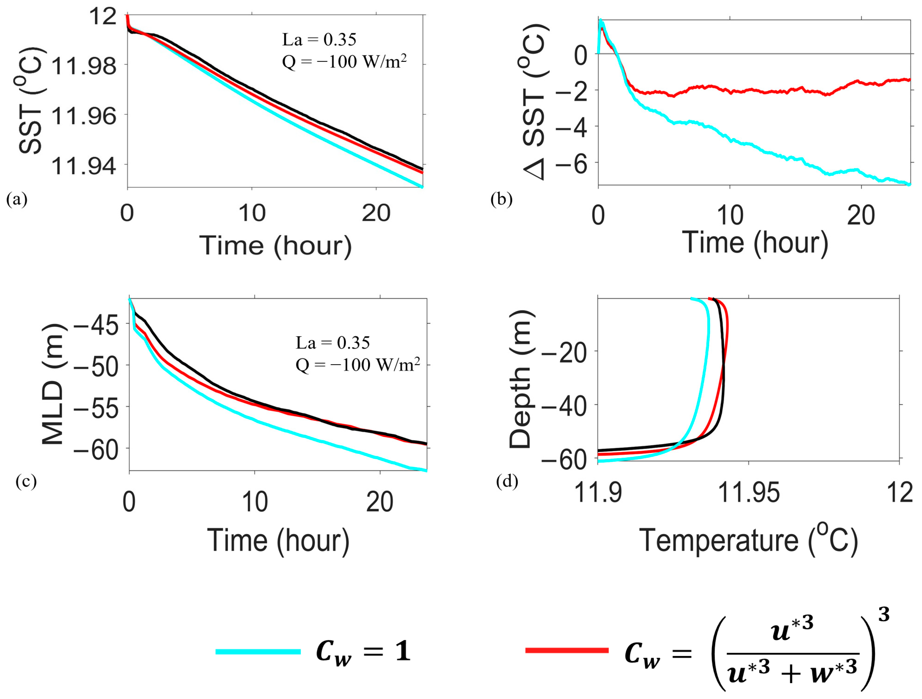
Take the LES Case 7 with surface cooling rate of 100 W/m2 (Section 3.1, Table 1) as an example. To better illustrate the role of the weighting factor (Equation (6)), we conduct a comparison experiment, where is set to 1, namely, no attenuation of Langmuir enhancement factor under convection.
According to the model results, when , the simulated MLD is much deeper than the LES outcome (Figure A1c), and the simulated temperature exhibits a larger cold bias compared to LES results (Figure A1a,d), both implying excessive mixing with .
By contrast, with , both the simulated MLD and temperature align more closely with the LES results. Namely, incorporating convective effects via helps dynamically balance the competition between Langmuir turbulence and convective turbulence, thereby preventing an overestimation of vertical mixing.
Figure A1.
LES with idealized forcing (Section 3.1, Case 7) with (no attenuation of Langmuir mixing) and . (a) Sea surface temperature, (b) sea surface temperature difference, (c) mixed layer depth, and (d) temperature profiles at the end of the simulations. Black lines represent the LES results.
References
- Craik, A.D.D.; Leibovich, S. A rational model for Langmuir circulations. J. Fluid Mech. 1976, 73, 401–426. [Google Scholar] [CrossRef] [Scilit]
- McWilliams, J.C.; Sullivan, P.P.; Moeng, C.H. Langmuir turbulence in the ocean. J. Fluid Mech. 1997, 334, 1–30. [Google Scholar] [CrossRef] [Scilit]
- Wang, P.; Özgökmen, T.M. Langmuir Circulation With Explicit Surface Waves From Moving-Mesh Modeling. Geophys. Res. Lett. 2018, 45, 216–226. [Google Scholar] [CrossRef] [Scilit]
- Langmuir, I. Surface Motion of Water Induced by Wind. Science 1938, 87, 119–123. [Google Scholar] [CrossRef] [Scilit] [PubMed]
- Thorpe, S.A. Langmuir Circulation. Annu. Rev. Fluid Mech. 2004, 36, 55–79. [Google Scholar] [CrossRef] [Scilit]
- Chen, B.C.; Yang, D.; Meneveau, C.; Chamecki, M. Effects of swell on transport and dispersion of oil plumes within the ocean mixed layer. J. Geophys. Res. Oceans 2016, 121, 3564–3578. [Google Scholar] [CrossRef] [Scilit]
- Gargett, A.; Wells, J.; Tejada-Martinez, A.E.; Grosch, C.E. Langmuir supercells: A mechanism for sediment resuspension and transport in shallow seas. Science 2004, 306, 1925–1928. [Google Scholar] [CrossRef] [Scilit]
- Kukulka, T.; Plueddemann, A.J.; Trowbridge, J.H.; Sullivan, P.P. Significance of Langmuir circulation in upper ocean mixing: Comparison of observations and simulations. Geophys. Res. Lett. 2009, 36, L10603. [Google Scholar] [CrossRef] [Scilit]
- Yang, D.; Chen, B.; Chamecki, M.; Meneveau, C. Oil plumes and dispersion in Langmuir, upper-ocean turbulence: Large-eddy simulations and K-profile parameterization. J. Geophys. Res. Oceans 2015, 120, 4729–4759. [Google Scholar] [CrossRef] [Scilit]
- Wu, J.; Wang, P. Langmuir Turbulence Effects on Coastal Surface Waves. J. Mar. Sci. Eng. 2025, 13, 1067. [Google Scholar] [CrossRef] [Scilit]
- Ali, A.; Christensen, K.H.; Breivik, O.; Malila, M.; Raj, R.P.; Bertino, L.; Chassignet, E.P.; Bakhoday-Paskyabi, M. A comparison of Langmuir turbulence parameterizations and key wave effects in a numerical model of the North Atlantic and Arctic Oceans. Ocean Model. 2019, 137, 76–97. [Google Scholar] [CrossRef] [Scilit]
- Li, Q.; Reichl, B.G.; Fox-Kemper, B.; Adcroft, A.J.; Belcher, S.E.; Danabasoglu, G.; Grant, A.L.M.; Griffies, S.M.; Hallberg, R.; Hara, T.; et al. Comparing Ocean Surface Boundary Vertical Mixing Schemes Including Langmuir Turbulence. J. Adv. Model. Earth Syst. 2019, 11, 3545–3592. [Google Scholar] [CrossRef] [Scilit]
- McWilliams, J.C.; Sullivan, P.P. Vertical Mixing by Langmuir Circulations. Spill Sci. Technol. Bull. 2000, 6, 225–237. [Google Scholar] [CrossRef] [Scilit]
- Wang, P.; McWilliams, J.C.; Yuan, J.G.; Liang, J.H. Langmuir Mixing Schemes Based on a Modified K-Profile Parameterization. J. Adv. Model. Earth Syst. 2025, 17, e2024MS004729. [Google Scholar] [CrossRef] [Scilit]
- Large, W.G.; McWilliams, J.C.; Doney, S.C. Oceanic vertical mixing: A review and a model with a nonlocal boundary layer parameterization. Rev. Geophys. 1994, 32, 363–403. [Google Scholar] [CrossRef] [Scilit]
- Harcourt, R.R. An Improved Second-Moment Closure Model of Langmuir Turbulence. J. Phys. Oceanogr. 2015, 45, 84–103. [Google Scholar] [CrossRef] [Scilit]
- Solano, M.; Fan, Y.L. A new K-profile parameterization for the ocean surface boundary layer under realistic forcing conditions. Ocean Model. 2022, 171, 101958. [Google Scholar] [CrossRef] [Scilit]
- Harcourt, R.R.; D’Asaro, E.A. Large-eddy simulation of Langmuir turbulence in pure wind seas. J. Phys. Oceanogr. 2008, 38, 1542–1562. [Google Scholar] [CrossRef] [Scilit]
- Van Roekel, L.P.; Fox-Kemper, B.; Sullivan, P.P.; Hamlington, P.E.; Haney, S.R. The form and orientation of Langmuir cells for misaligned winds and waves. J. Geophys. Res. Oceans 2012, 117, C05001. [Google Scholar] [CrossRef] [Scilit]
- Fan, Y.L.; Griffies, S.M. Impacts of Parameterized Langmuir Turbulence and Nonbreaking Wave Mixing in Global Climate Simulations. J. Clim. 2014, 27, 4752–4775. [Google Scholar] [CrossRef] [Scilit]
- Grant, A.L.M.; Belcher, S.E. Characteristics of Langmuir Turbulence in the Ocean Mixed Layer. J. Phys. Oceanogr. 2009, 39, 1871–1887. [Google Scholar] [CrossRef] [Scilit]
- Kantha, L.H.; Anne Clayson, C. On the effect of surface gravity waves on mixing in the oceanic mixed layer. Ocean Model. 2004, 6, 101–124. [Google Scholar] [CrossRef] [Scilit]
- Smyth, W.D.; Skyllingstad, E.D.; Crawford, G.B.; Wijesekera, H. Nonlocal fluxes and Stokes drift effects in the K-profile parameterization. Ocean Dyn. 2002, 52, 104–115. [Google Scholar] [CrossRef] [Scilit]
- Frech, M.; Mahrt, L. A two-scale mixing formulation for the atmospheric boundary layer. Bound.-Layer Meteorol. 1995, 73, 91–104. [Google Scholar] [CrossRef] [Scilit]
- Noh, Y.; Cheon, W.G.; Hong, S.Y.; Raasch, S. Improvement of the K-profile Model for the Planetary Boundary Layer based on Large Eddy Simulation Data. Bound.-Layer Meteorol. 2003, 107, 401–427. [Google Scholar] [CrossRef] [Scilit]
- Li, Q.; Fox-Kemper, B. Assessing the Effects of Langmuir Turbulence on the Entrainment Buoyancy Flux in the Ocean Surface Boundary Layer. J. Phys. Oceanogr. 2017, 47, 2863–2886. [Google Scholar] [CrossRef] [Scilit]
- Yuan, J.; Liang, J.-H.; Chassignet, E.P.; Zavala-Romero, O.; Wan, X.; Cronin, M.F. The K-profile parameterization augmented by deep neural networks (KPP_DNN) in the general ocean turbulence model (GOTM). J. Adv. Model. Earth Syst. 2024, 16, e2024MS004405. [Google Scholar] [CrossRef] [Scilit]

Disclaimer/Publisher’s Note: The statements, opinions and data contained in all publications are solely those of the individual author(s) and contributor(s) and not of MDPI and/or the editor(s). MDPI and/or the editor(s) disclaim responsibility for any injury to people or property resulting from any ideas, methods, instructions or products referred to in the content. |
© 2026 by the authors. Licensee MDPI, Basel, Switzerland. This article is an open access article distributed under the terms and conditions of the Creative Commons Attribution (CC BY) license.