Reconstruction Support and Island Dominance in Black-Hole Information Recovery

Abstract

The island formula recovers a unitary Page curve in controlled gravitational models, but the dominance of an island saddle, the existence of a radiation recovery channel, and the cost of implementing that channel are logically distinct statements. We formulate this distinction as a two-stage framework. In the first stage, candidate islands and the physical Page transition are determined exclusively by the standard generalized entropy and quantum-extremal-surface (QES) prescription. In the second stage, an explicitly model-dependent reconstruction score ranks the QES candidates by normalized recovery, connectivity, algebraic, and complexity diagnostics. The score is not proposed as a new gravitational entropy formula. For a nondegenerate island/no-island crossing we derive the first- and second-order displacement of the operational reconstruction-support transition relative to the Page transition. We define operator recovery on a code subspace without assuming an interior–exterior tensor factorization, state the Fawzi–Renner recoverability implication with its correct conditional-mutual-information hypothesis, and derive a dimension-normalized mutual-information network diagnostic bounded in $\left[0,1\right]$. We then test the diagnostics in a fully reproducible random-Clifford evaporation model. A self-contained binary stabilizer calculation uses n = 12, 16, and 20 black-hole qubits and 256 seeded realizations per size and ensemble. The entropy peak converges to an emitted fraction k/n = 1/2, whereas a reference qubit becomes equally correlated with radiation and the remaining register near the same point. A stricter decoupling criterion occurs later. Pairwise radiation–network connectivity and multipartite total correlation exhibit sharply different behavior, demonstrating that a pairwise network cannot by itself certify interior reconstruction. These results support reconstruction support as an operational layer placed on top of—not inside—the island rule, and they give falsifiable criteria for future tensor-network, random-circuit, and semiclassical calculations.

1. Introduction

The black-hole information problem begins with a precise tension. Semiclassical quantum field theory predicts approximately thermal Hawking radiation from a black hole [1,2]. If an initially pure collapsing state evaporated into an exactly thermal density operator, the map

$$|{\Psi }_{\mathrm{i}\mathrm{n}}⟩⟨{\Psi }_{\mathrm{i}\mathrm{n}}|\to {\rho }_{\mathrm{r}\mathrm{a}\mathrm{d}}, S\left({\rho }_{\mathrm{r}\mathrm{a}\mathrm{d}}\right)>0,$$

(1)

would not be unitary. Page converted this qualitative conflict into an entropy benchmark [3,4]. For a globally pure black-hole–radiation state,

$$S\left(R_t\right)=S\left(B_t\right),$$

(2)

so the fine-grained radiation entropy must eventually decrease as the remaining black hole becomes the smaller subsystem. The resulting Page curve is now reproduced in tractable gravitational models by QESs, islands, and replica wormholes [5,6,7,8,9,10,11].

This article works within the standard semiclassical framework of Hawking radiation and black-hole thermodynamics [1,12,13]. In this framework, the black hole is described geometrically, and the Page curve tracks the von Neumann entropy of the radiation subsystem; the quantity analyzed here is not a local material entropy assigned to the black-hole interior. The paper asks how generalized-entropy saddle selection relates to operational recovery within this declared framework. Models founded on different assumptions, including models that do not adopt semiclassical black-hole thermodynamics, lie outside the scope of the present analysis.

The success of the entropy calculation does not make every statement about information recovery equivalent. Three logically distinct questions should therefore be separated. One asks which gravitational saddle computes the fine-grained entropy of the radiation. A second asks whether a channel or radiation operator reconstructs a chosen logical interior degree of freedom on a specified code subspace and with a specified error. The third concerns the resources and wall-clock time required to implement that recovery.

The island formula answers the first question. Entanglement-wedge reconstruction and quantum error correction address the second [14,15,16]. The third is constrained by the Hayden–Preskill protocol, the Harlow–Hayden complexity obstruction, and related geometric proposals [17,18,19,20]. Conflating the three can turn a useful operational diagnostic into an unjustified modification of the gravitational entropy.

This paper develops a reconstruction-support framework while enforcing that separation. The original motivation is retained: semiclassical spatial regions in gravity should not automatically be identified with exact Hilbert-space tensor factors, and the location of information is often best stated in terms of reconstructible operator algebras. The implementation, however, is deliberately conservative. Candidate islands are first obtained from the standard QES equations. Complexity, correlation connectivity, and algebraic nonfactorization then enter a second-stage operational score. They do not move a physical QES unless an independent gravitational effective action supplies the corresponding deformation.

The principal contribution is a two-stage definition that prevents a phenomenological gate count or graph statistic from being mistaken for a term in gravitational generalized entropy. Building on this separation, we derive the displacement of a reconstruction-support crossing through second order, state the nondegeneracy and small-deformation hypotheses, and distinguish the resulting time from both the Page time and the decoder completion time. We also formulate state and operator reconstruction with type-consistent channels and code-subspace norms, replacing a previously overstrong ordinary-mutual-information ansatz with the precise conditional-mutual-information recoverability statement. For the correlation analysis, we prove a bounded normalization for the mutual-information network and add total correlation as a multipartite diagnostic that exposes information missed by pairwise edges. Finally, we supply a deterministic, external-package-free stabilizer simulation together with raw and aggregated data, a finite-size comparison, uncertainty estimates, and exact internal consistency tests.

The scope is correspondingly limited. The operational score is a structured ansatz, not a replica path-integral derivation. The Clifford model is a quantum-information testbed, not a simulation of semiclassical gravity. The results therefore establish consistency, clarify implications, and produce concrete diagnostics; they do not derive the island rule from the reconstruction score or resolve every assumption in the firewall argument.

2. Established Entropy and Reconstruction Ingredients

2.1. Page’s Typical-State Benchmark

Let $\mathcal{H}={\mathcal{H}}_R\otimes {\mathcal{H}}_B$ with dimensions $m=\mathrm{d}\mathrm{i}\mathrm{m}{\mathcal{H}}_R$ and $n=\mathrm{d}\mathrm{i}\mathrm{m}{\mathcal{H}}_B$, and take $m\le n$. For a Haar-random pure state, Page’s exact average entropy of the smaller subsystem is as follows:

$$\mathbb{E}S\left(R\right)={\displaystyle \sum _{j=n+1}^{mn}}{\displaystyle \frac{1}{j}}-{\displaystyle \frac{m-1}{2n}},$$

(3)

in natural-logarithm units [3]. Expanding the harmonic numbers gives the following:

$$\mathbb{E}S\left(R\right)=\mathrm{l}\mathrm{o}\mathrm{g}m-{\displaystyle \frac{m^2-1}{2mn}}+O\left(n^{-2}\right),$$

(4)

where the displayed correction is useful only in the regime for which the expansion is controlled. Interchanging $m$ and $n$ after the two dimensions cross produces the familiar typical-state Page curve. This is a kinematic benchmark; it does not by itself identify a bulk surface or construct a decoder.

A common continuous toy model writes the two competing branches as follows:

$$S_{\mathrm{n}\mathrm{o}}\left(t\right)=\alpha t, S_{\mathrm{i}\mathrm{s}}\left(t\right)=S_0-\alpha t,$$

(5)

with $\alpha >0$. Their crossing occurs at the following:

$$t_{\mathrm{P}\mathrm{a}\mathrm{g}\mathrm{e}}^{\left(0\right)}={\displaystyle \frac{S_0}{2\alpha }}.$$

(6)

Equation (5) is not a detailed four-dimensional evaporation law: it suppresses greybody factors, the distinction between thermodynamic and von Neumann entropy fluxes, and the time dependence of the Hawking temperature. We use it only after deriving the general saddle-difference formula.

2.2. Generalized Entropy, QESs, and Islands

For a candidate surface $X$, the generalized entropy is as follows:

$$S_{\mathrm{g}\mathrm{e}\mathrm{n}}\left[X\right]={\displaystyle \frac{\mathrm{A}\mathrm{r}\mathrm{e}\mathrm{a}\left(X\right)}{4G_N\mathrm{\hslash }}}+S_{\mathrm{b}\mathrm{u}\mathrm{l}\mathrm{k}}\left[X\right]+S_{\mathrm{c}\mathrm{t}}\left[X\right],$$

(7)

where counterterms render the sum finite in a specified renormalization scheme. A QES satisfies the following:

$${\displaystyle \frac{\delta S_{\mathrm{g}\mathrm{e}\mathrm{n}}}{\delta X}}=0.$$

(8)

For radiation $R$ coupled to a gravitating region, the island prescription is schematically as follows:

$$S\left(R\right)=\underset{I\in {\mathcal{Q}}_R}{\mathrm{m}\mathrm{i}\mathrm{n}}\left[{\displaystyle \frac{\mathrm{A}\mathrm{r}\mathrm{e}\mathrm{a}\left(\partial I\right)}{4G_N\mathrm{\hslash }}}+S_{\mathrm{m}\mathrm{a}\mathrm{t}\mathrm{t}\mathrm{e}\mathrm{r}}\left(R\cup I\right)+S_{\mathrm{c}\mathrm{t}}\left(\partial I\right)\right],$$

(9)

where ${\mathcal{Q}}_R$ is the set of admissible extrema obeying homology and boundary conditions. The order matters: one extremizes first and minimizes over extrema second. In controlled models the late-time island saddle follows from replica-wormhole contributions to the gravitational path integral, not from inserting an arbitrary measure of decoding difficulty [9,10].

Let $I_0=\mathrm{⌀}$ and $I_1\ne \mathrm{⌀}$ denote the relevant no-island and island candidates. Define as follows:

$$\Delta S_{\mathrm{g}\mathrm{e}\mathrm{n}}\left(t\right)=S_{\mathrm{g}\mathrm{e}\mathrm{n}}\left[I_1;R_t\right]-S_{\mathrm{g}\mathrm{e}\mathrm{n}}\left[I_0;R_t\right].$$

(10)

The physical saddle exchange is as follows:

$$\Delta S_{\mathrm{g}\mathrm{e}\mathrm{n}}\left(t_{\mathrm{P}\mathrm{a}\mathrm{g}\mathrm{e}}\right)=0, {\dot{\Delta S}}_{\mathrm{g}\mathrm{e}\mathrm{n}}\left(t_{\mathrm{P}\mathrm{a}\mathrm{g}\mathrm{e}}\right)\ne 0$$

(11)

for a nondegenerate crossing. This definition, rather than any operational deformation below, sets the Page time throughout the paper.

2.3. Entanglement Wedge and Code-Subspace Reconstruction

In holography, a bulk operator in the entanglement wedge of a boundary region can be represented on that boundary region under appropriate code-subspace assumptions [15,16]. Let the following:

$$V:{\mathcal{H}}_{\mathrm{c}\mathrm{o}\mathrm{d}\mathrm{e}}\to {\mathcal{H}}_R\otimes {\mathcal{H}}_B$$

(12)

be an encoding isometry. An exact radiation representative $O_R$ of a logical operator $O$ obeys the following:

$$\left(O_R\otimes {\mathsf{1}}_B\right)V=VO.$$

(13)

Multiple representatives on different physical subsystems do not constitute independent copies: they agree on the image of $V$. This is the precise code-subspace statement behind the phrase “the interior becomes reconstructible from the radiation.”

Gravity adds a further reason for caution about tensor factors. Gauge constraints and gravitational dressing obstruct canonical factorization by coordinate subregions. Operator algebras, centers, edge data, and a specified code subspace are therefore safer primitives than a literal identity ${\mathcal{H}}_{\mathrm{i}\mathrm{n}\mathrm{s}\mathrm{i}\mathrm{d}\mathrm{e}}\otimes {\mathcal{H}}_{\mathrm{o}\mathrm{u}\mathrm{t}\mathrm{s}\mathrm{i}\mathrm{d}\mathrm{e}}$. The operational framework below is written so that it does not require such an identity.

3. A Two-Stage Reconstruction-Support Framework

3.1. Stage One: The Gravitational Candidate Set

For each time $t$, solve the standard QES problem and collect all admissible extrema in the following:

$$\mathcal{Q}\left(t\right)=\left\{I_a\left(t\right):{\left.{\displaystyle \frac{\delta S_{\mathrm{g}\mathrm{e}\mathrm{n}}\left[I;R_t\right]}{\delta I}}\right|}_{I=I_a}=0,\hspace{0.25em}{I}_a\mathrm{satisfies}\mathrm{the}\mathrm{boundary}\mathrm{and}\mathrm{homology}\mathrm{conditions}\right\}.$$

(14)

The physical island is as follows:

$$I_{\mathrm{p}\mathrm{h}\mathrm{y}\mathrm{s}}\left(t\right)=\mathrm{a}\mathrm{r}\mathrm{g}\underset{I_a\in \mathcal{Q}\left(t\right)}{\mathrm{m}\mathrm{i}\mathrm{n}}{S}_{\mathrm{g}\mathrm{e}\mathrm{n}}\left[I_a;R_t\right].$$

(15)

No circuit gate count, mutual-information graph, or algebraic penalty is used in (14) and (15). This restriction is essential: without a gravitational path-integral or effective-action derivation, adding those quantities to $S_{\mathrm{g}\mathrm{e}\mathrm{n}}$ would change the asserted physics without controlling the change.

3.2. Stage Two: An Operational Score on QES Candidates

For a candidate $I_a\in \mathcal{Q}\left(t\right)$, define a dimensionless feature vector as follows:

$${\mathbf{f}}_a\left(t\right)=\left(c_a\left(t\right),d_a\left(t\right),g_a\left(t\right),a_a\left(t\right)\right),$$

(16)

where

$$c_a=\mathrm{l}\mathrm{o}\mathrm{g}\left(1+{\displaystyle \frac{C_a^{\left(\epsilon \right)}}{C_0}}\right),\mathrm{normalized}\mathrm{decoder}\mathrm{complexity},$$

(17)

$$d_a=-\mathrm{l}\mathrm{o}\mathrm{g}{F}_a^2,\mathrm{recovery}\mathrm{infidelity}\mathrm{cost},$$

(18)

$$0\le g_a\le 1,\mathrm{normalized}\mathrm{correlation}\mathrm{connectivity},$$

(19)

$$a_a\ge 0,\mathrm{algebraic}/\mathrm{nonfactorization}\mathrm{obstruction}.$$

(20)

Here, $C_a^{\left(\epsilon \right)}$ is the minimum gate count among decoders reaching a declared error tolerance $\epsilon$, $C_0$ fixes the dimensionless convention, and $F_a$ is a state-recovery fidelity in a specified experiment. The quantities are undefined until the code subspace, allowed gates, reference state or state family, and error metric are given. In particular, they are not universal properties of a coordinate region.

The reconstruction cost is as follows:

$${\Phi }_{\mathrm{r}\mathrm{e}\mathrm{c}}\left(I_a;R_t\right)=w_c{c}_a+w_d{d}_a-w_g{g}_a+w_a{a}_a, w_c,w_d,w_g,w_a\ge 0,$$

(21)

and the operational reconstruction score is as follows:

$${\mathcal{J}}_{\mathrm{r}\mathrm{e}\mathrm{c}}\left(I_a;R_t\right)=S_{\mathrm{g}\mathrm{e}\mathrm{n}}\left(I_a;R_t\right)+\mu {\Phi }_{\mathrm{r}\mathrm{e}\mathrm{c}}\left(I_a;R_t\right), I_a\in \mathcal{Q}\left(t\right).$$

(22)

The scale $\mu$ has entropy units. It is a conversion parameter fixed by the operational task, not a new gravitational coupling. Because ${\mathcal{J}}_{\mathrm{r}\mathrm{e}\mathrm{c}}$ is evaluated only after the QES candidate set has been found, it cannot create or relocate a physical QES.

Definition 1 

(Reconstruction-support transition). For two continuously tracked candidates $I_0\left(t\right)$ and  $I_1\left(t\right)$, define  $\Delta J\left(t,\mu \right)={\mathcal{J}}_{\mathrm{r}\mathrm{e}\mathrm{c}}\left(I_1;R_t\right)-{\mathcal{J}}_{\mathrm{r}\mathrm{e}\mathrm{c}}\left(I_0;R_t\right).$ A reconstruction-support transition is a nondegenerate zero  $\Delta J\left(t_{\mathrm{r}\mathrm{e}\mathrm{c}},\mu \right)=0$. It is an operational crossover and need not coincide with the physical Page transition.

This definition retains the useful competition in the original reconstruction-functional idea while removing an ambiguity: $t_{\mathrm{P}\mathrm{a}\mathrm{g}\mathrm{e}}$ is a property of the gravitational entropy calculation, whereas $t_{\mathrm{r}\mathrm{e}\mathrm{c}}$ depends on the declared recovery task and its weights.

3.3. Explicit Island/No-Island Support Criterion

The central saddle comparison can be retained in a bounded operational form. Let subscripts zero and one denote the no-island and island candidates, respectively, and write $\Delta x=x_1-x_0$ for every feature. From (22),

$$\Delta J=\Delta S_{\mathrm{g}\mathrm{e}\mathrm{n}}+\mu \left(w_c\Delta c+w_d\Delta d-w_g\Delta g+w_a\Delta a\right).$$

(23)

The island candidate has smaller operational score exactly when

$$\Delta S_{\mathrm{g}\mathrm{e}\mathrm{n}}+\mu \left(w_c\Delta c+w_d\Delta d+w_a\Delta a\right)<\mu w_g\Delta g.$$

(24)

For $\mu w_g>0$, this becomes the explicit connectivity threshold as follows:

$$\boxed{\Delta g>g_{\mathrm{c}\mathrm{r}\mathrm{i}\mathrm{t}}\equiv {\displaystyle \frac{\Delta S_{\mathrm{g}\mathrm{e}\mathrm{n}}}{\mu w_g}}+{\displaystyle \frac{w_c\Delta c+w_d\Delta d+w_a\Delta a}{w_g}}}.$$

(25)

Equation (25) is the corrected counterpart of an unnormalized mutual-information threshold. It compares an island connectivity advantage with its geometric, fidelity, complexity, and algebraic disadvantages. Because $g_0,g_1\in \left[0,1\right]$, one has $-1\le \Delta g\le 1$. Therefore, $g_{\mathrm{c}\mathrm{r}\mathrm{i}\mathrm{t}}>1$ rules out an operational island advantage for the declared weights, while $g_{\mathrm{c}\mathrm{r}\mathrm{i}\mathrm{t}}<-1$ makes the condition automatic. These feasibility checks were absent when raw mutual information with an unrestricted dimension was subtracted from the score.

At the physical Page time, $\Delta S_{\mathrm{g}\mathrm{e}\mathrm{n}}=0$, but (25) can still fail if the island decoder is too costly or inaccurate for the chosen task. Conversely, sufficiently favorable recovery and connectivity features can produce $t_{\mathrm{r}\mathrm{e}\mathrm{c}}<t_{\mathrm{P}\mathrm{a}\mathrm{g}\mathrm{e}}$ as a ranking statement, but they do not make the island the physical entropy saddle before $t_{\mathrm{P}\mathrm{a}\mathrm{g}\mathrm{e}}$.

3.4. Why the Bounded Normalization Matters

An unnormalized negative mutual-information term does not make a functional bounded below merely because its coefficient is smaller than $1/2$. Consider a maximally entangled state on two $d$-dimensional factors $I$ and $R$. Then

$$S\left(IR\right)=0, I\left(I:R\right)=2\mathrm{l}\mathrm{o}\mathrm{g}d.$$

(26)

Consequently, $S\left(IR\right)-\lambda I\left(I:R\right)=-2\lambda \mathrm{l}\mathrm{o}\mathrm{g}d$, which tends to $-\mathrm{\infty }$ with $d$ for every $\lambda >0$. Subadditivity does not give the claimed lower bound.

There are two clean repairs. The present framework minimizes over a prescribed, finite or compact set of QES candidates and uses a dimension-normalized $g_a\in \left[0,1\right]$. Alternatively, a microscopic theory may provide a coercive complexity or area term with a proved scaling relation. Absent either repair, a negative connectivity reward is a heuristic expression rather than a well-defined variational principle.

4. Transition Displacement and Its Domain of Validity

4.1. First-Order Displacement

For the island/no-island pair, write the following:

$$\Delta J\left(t,\mu \right)=f\left(t\right)+\mu g\left(t\right), f\left(t\right)=\Delta S_{\mathrm{g}\mathrm{e}\mathrm{n}}\left(t\right), g\left(t\right)=\Delta {\Phi }_{\mathrm{r}\mathrm{e}\mathrm{c}}\left(t\right).$$

(27)

Let $t_0=t_{\mathrm{P}\mathrm{a}\mathrm{g}\mathrm{e}}$ satisfy $f\left(t_0\right)=0$ and $f^{\prime }\left(t_0\right)\ne 0$. The implicit-function theorem then guarantees a unique differentiable root $t\left(\mu \right)$ in a neighborhood of $\mu =0$. Differentiating

$$f\left(t\left(\mu \right)\right)+\mu g\left(t\left(\mu \right)\right)=0$$

(28)

gives

$$\left[f^{\prime }\left(t\right)+\mu g^{\prime }\left(t\right)\right]t^{\prime }\left(\mu \right)+g\left(t\right)=0.$$

(29)

At $\mu =0$,

$$t^{\prime }\left(0\right)=-{\displaystyle \frac{g\left(t_0\right)}{f^{\prime }\left(t_0\right)}}.$$

(30)

Therefore,

$$\boxed{t_{\mathrm{r}\mathrm{e}\mathrm{c}}=t_{\mathrm{P}\mathrm{a}\mathrm{g}\mathrm{e}}-\mu {\displaystyle \frac{\Delta {\Phi }_{\mathrm{r}\mathrm{e}\mathrm{c}}\left(t_{\mathrm{P}\mathrm{a}\mathrm{g}\mathrm{e}}\right)}{{\dot{\Delta S}}_{\mathrm{g}\mathrm{e}\mathrm{n}}\left(t_{\mathrm{P}\mathrm{a}\mathrm{g}\mathrm{e}}\right)}}+O\left({\mu }^2\right)}.$$

(31)

The numerator is task-dependent; the denominator is fixed by physical saddle competition. Equation (31) is meaningful only if both candidates can be tracked smoothly through the crossing and the correction remains small on the time scale over which $f$ varies.

4.2. Second-Order Correction

The full derivation is short enough to retain. Differentiate (29) once more:

$$\left[f^{\prime }\left(t\right)+\mu g^{\prime }\left(t\right)\right]t^{″}+\left[f^{″}\left(t\right)+\mu g^{″}\left(t\right)\right]{\left(t^{\prime }\right)}^2+2g^{\prime }\left(t\right)t\prime =0.$$

(32)

At $\mu =0$, set $a=t^{\prime }\left(0\right)=-g_0/f_1$, where $f_j=f^{\left(j\right)}\left(t_0\right)$ and $g_j=g^{\left(j\right)}\left(t_0\right)$. Then,

$$t^{″}\left(0\right)=-{\displaystyle \frac{f_2{a}^2+2g_{1}a}{f_1}}.$$

(33)

Taylor expansion yields the following:

$$t_{\mathrm{r}\mathrm{e}\mathrm{c}}=t_0+\mu a-{\displaystyle \frac{{\mu }^2}{2f_1}}\left(f_2{a}^2+2g_{1}a\right)+O\left({\mu }^3\right).$$

(34)

The $g_1$ term records the evolution of the reconstruction task itself. It cannot be inferred from the Page curve. The $f_2$ term records curvature of the physical saddle difference. Reporting only a constant additive shift is justified when both are negligible over the inferred displacement.

4.3. Linear-Branch Limit

For (5), the island-minus-no-island difference is as follows:

$$f\left(t\right)=S_0-2\alpha t, f^{\prime }\left(t\right)=-2\alpha .$$

(35)

If $g\left(t\right)=\Delta {\Phi }_0$ is constant near the crossing, the operational crossing can be solved exactly:

$$0=S_0-2\alpha t_{\mathrm{r}\mathrm{e}\mathrm{c}}+\mu \Delta {\Phi }_0,$$

(36)

so

$$\boxed{t_{\mathrm{r}\mathrm{e}\mathrm{c}}={\displaystyle \frac{S_0}{2\alpha }}+{\displaystyle \frac{\mu \Delta {\Phi }_0}{2\alpha }}}.$$

(37)

A positive net operational cost for the island candidate delays the support crossover; a sufficiently large normalized connectivity reward advances it. This is not a corrected physical Page time. It is a corrected operational crossing built on an unchanged Page time.

4.4. Uncertainty and Failure Modes

Suppose $g_0$ and $f_1$ have small uncertainties ${\sigma }_g$ and ${\sigma }_f$ with covariance $\mathrm{C}\mathrm{o}\mathrm{v}\left(g_0,f_1\right)$. Linear error propagation gives the following:

$${\sigma }_{\delta t}^2\simeq {\mu }^2\left[{\displaystyle \frac{{\sigma }_g^2}{f_1^2}}+{\displaystyle \frac{g_0^2{\sigma }_f^2}{f_1^4}}-{\displaystyle \frac{2g_0\mathrm{C}\mathrm{o}\mathrm{v}\left(g_0,f_1\right)}{f_1^3}}\right].$$

(38)

The perturbative calculation fails near a tangent or higher-order crossing $f_1\approx 0$, at a discontinuous change in the candidate set, or when $\left|\mu g_0/f_1\right|$ is comparable to the time scale on which $f_1$ or $g$ changes. In those cases, the full score must be solved without expanding, and the result should still be labeled operational.

5. Recovery Statements with Type-Consistent Errors

5.1. State Recovery

Let $V$ be the encoding isometry in (12). The radiation channel is as follows:

$${\mathcal{N}}_R\left(\rho \right)={\mathrm{T}\mathrm{r}}_B\left(V\rho V^{†}\right).$$

(39)

For a declared family $\mathfrak{S}$ of code states and a decoder ${\mathcal{D}}_R:\mathcal{L}\left({\mathcal{H}}_R\right)\to \mathcal{L}\left({\mathcal{H}}_{\mathrm{c}\mathrm{o}\mathrm{d}\mathrm{e}}\right)$, define the following:

$${\epsilon }_{\mathrm{s}\mathrm{t}\mathrm{a}\mathrm{t}\mathrm{e}}\left({\mathcal{D}}_R;\mathfrak{S}\right)=\underset{\rho \in \mathfrak{S}}{\mathrm{s}\mathrm{u}\mathrm{p}}P\left(\rho ,\left({\mathcal{D}}_R\circ {\mathcal{N}}_R\right)\left(\rho \right)\right),$$

(40)

where $P\left(\rho ,\sigma \right)=\sqrt{1-F{\left(\rho ,\sigma \right)}^2}$ is the purified distance and $F$ denotes root fidelity. The minimum complexity at tolerance $\epsilon$ is as follows:

$$C_R^{\left(\epsilon \right)}=\underset{{\mathcal{D}}_R:\hspace{0.17em}{\epsilon }_{\mathrm{s}\mathrm{t}\mathrm{a}\mathrm{t}\mathrm{e}}\le \epsilon }{\mathrm{i}\mathrm{n}\mathrm{f}}\mathrm{G}\mathrm{a}\mathrm{t}\mathrm{e}\mathrm{C}\mathrm{o}\mathrm{u}\mathrm{n}\mathrm{t}\left({\mathcal{D}}_R\right).$$

(41)

This quantity depends on the gate set, ancilla and precision conventions, and state family. Writing it without those declarations creates a formally compact but physically ambiguous term.

5.2. Operator Reconstruction

For a logical operator $O$ with $\parallel O\parallel \le 1$, a type-consistent code-subspace error is

$${\epsilon }_R\left(O\right)=\underset{O_R\in \mathcal{A}\left(R\right)}{\mathrm{i}\mathrm{n}\mathrm{f}}∥VO-\left(O_R\otimes {\mathsf{1}}_B\right)V∥,$$

(42)

or, equivalently, a projected norm on $P=V{V}^{†}$. The earlier schematic expression $\parallel O_I-{\mathrm{R}\mathrm{e}\mathrm{c}}_R\left(O_I\right)\parallel$ is not generally well-typed: a Schrödinger-picture recovery channel acts on states, while a reconstructed operator is obtained from an adjoint channel or by the infimum in (42). Equation (42) also makes the code-subspace restriction explicit.

5.3. What Fawzi–Renner Does and Does Not Imply

For a tripartite state ${\rho }_{ABC}$, the conditional mutual information in bits is

$$I{\left(A:C|B\right)}_{\rho }=S\left(AB\right)+S\left(BC\right)-S\left(B\right)-S\left(ABC\right).$$

(43)

The Fawzi–Renner theorem implies the existence of a channel ${\mathcal{R}}_{B\to BC}$ such that, with root-fidelity convention,

$$I{\left(A:C|B\right)}_{\rho }\ge -2{\mathrm{l}\mathrm{o}\mathrm{g}}_{2}F\left({\rho }_{ABC},{\mathcal{R}}_{B\to BC}\left({\rho }_{AB}\right)\right).$$

(44)

Thus, small conditional mutual information guarantees the existence of a good recovery map [21,22]. It does not establish a universal exponential relation between recovery error and ordinary mutual information $I\left(I:R\right)$. Ordinary mutual information measures total correlation; it does not specify the conditioning system or the channel whose missing output is to be reconstructed. Any formula of the form $\epsilon \sim e^{-\kappa I\left(I:R\right)}$ must therefore be labeled a model ansatz and independently tested.

In the operational score, one may use $d_a=-\mathrm{l}\mathrm{o}\mathrm{g}{F}_a^2$ obtained from an explicit decoder, or a conditional-mutual-information upper control when the tripartition and the recovery task match (44). A radiation-only pairwise graph is retained as a diagnostic, not promoted to a recovery theorem.

5.4. Reference Decoupling as a Direct Information-Transfer Test

Introduce a reference qubit $Q$ maximally entangled with a logical message before encoding. For the pure tripartite state on $QRB$,

$$I\left(Q:R\right)+I\left(Q:B\right)=2S\left(Q\right)=2\hspace{0.25em}\mathrm{bits}.$$

(45)

The identity follows by expanding the two mutual information and using $S\left(QR\right)=S\left(B\right)$ and $S\left(QB\right)=S\left(R\right)$. It provides an exact simulation check and a direct statement of where correlations with the logical reference reside.

Moreover,

$$I{\left(Q:B\right)}_{\rho }=D_2\left({\rho }_{QB}∥{\rho }_Q\otimes {\rho }_B\right),$$

(46)

where $D_2$ is quantum relative entropy with logarithm base two. Quantum Pinsker gives

$${∥{\rho }_{QB}-{\rho }_Q\otimes {\rho }_B∥}_1\le \sqrt{2\mathrm{l}\mathrm{n}2\hspace{0.17em}I\left(Q:B\right)}\equiv {\delta }_{\mathrm{d}\mathrm{e}\mathrm{c}}.$$

(47)

Small $I\left(Q:B\right)$ therefore certifies decoupling of the logical reference from the erased black-hole register. Standard information–disturbance/decoupling results then imply the existence of a recovery from $R$, with a convention-dependent conversion between decoupling distance and recovery error [23]. We plot ${\delta }_{\mathrm{d}\mathrm{e}\mathrm{c}}$ as a conservative product-state-distance certificate, not as the fidelity of an implemented optimal decoder.

The reference-qubit experiment used below is related to, but not identical to, the conventional Hayden–Preskill protocol [17]. In the standard Hayden–Preskill setup, a message system entangled with a reference is inserted into an old black hole that is already entangled with an explicitly retained early-radiation register; recovery is attempted from that early radiation together with the subsequently emitted radiation. By contrast, here the logical qubit is embedded in the initial black-hole register, no separate early-radiation side-information register is retained, and recovery is diagnosed from the accumulated radiation alone. Thus, the present experiment isolates the relevant decoupling and information-transfer logic but does not implement the full old-black-hole protocol.

6. Three Distinct Time Scales

The framework contains three time scales that should not be merged. The first is the standard generalized-entropy saddle exchange in (11). A second, task-dependent time is the zero of $\Delta J$, which marks when the selected radiation reconstruction becomes operationally preferable under specified weights. The third is the earliest time at which a physical observer completes a declared decoder.

For a message in a rapidly scrambling old black hole, a schematic access time is

$$t_{\mathrm{a}\mathrm{c}\mathrm{c}\mathrm{e}\mathrm{s}\mathrm{s}}\gtrsim t_{\mathrm{P}\mathrm{a}\mathrm{g}\mathrm{e}}+t_{\mathrm{s}\mathrm{c}\mathrm{r}}, t_{\mathrm{s}\mathrm{c}\mathrm{r}}\sim {\displaystyle \frac{\beta }{2\pi }}\mathrm{l}\mathrm{o}\mathrm{g}{S}_{\mathrm{B}\mathrm{H}},$$

(48)

with assumptions specific to the Hayden–Preskill setting. A decoder running at rate ${\Gamma }_{\mathrm{c}\mathrm{o}\mathrm{m}\mathrm{p}}$ then obeys the bookkeeping relation

$$t_{\mathrm{o}\mathrm{u}\mathrm{t}}=\mathrm{m}\mathrm{a}\mathrm{x}\{t_{\mathrm{a}\mathrm{c}\mathrm{c}\mathrm{e}\mathrm{s}\mathrm{s}},t_{\mathrm{r}\mathrm{e}\mathrm{c}}\}+{\displaystyle \frac{C_R^{\left(\epsilon \right)}}{{\Gamma }_{\mathrm{c}\mathrm{o}\mathrm{m}\mathrm{p}}}}.$$

(49)

The max prevents two threshold conditions from being added as if they were independent durations. The last term is wall-clock computational time. It is also not inserted into the Page entropy, avoiding double counting. For generic decoding tasks, the Harlow–Hayden argument permits $C_R^{\left(\epsilon \right)}$ to be exponentially large in the black-hole entropy even after the information is present in principle [18].

7. Conditional Geometric Deformation: A JT-Gravity Template

The two-stage construction does not move a QES. Nevertheless, the endpoint-shift algebra in the original proposal is useful in a different, conditional statement: if a microscopic calculation derives an additional term in a gravitational effective action, its effect on a QES can be evaluated perturbatively. This section makes that premise explicit.

In Jackiw–Teitelboim gravity coupled to matter, write a one-coordinate generalized entropy as

$$S_{\mathrm{g}\mathrm{e}\mathrm{n}}\left(x\right)={\displaystyle \frac{\varphi \left(x\right)}{4G_N}}+S_{\mathrm{m}\mathrm{a}\mathrm{t}\mathrm{t}\mathrm{e}\mathrm{r}}\left(R\cup I\left(x\right)\right)+S_{\mathrm{c}\mathrm{t}}\left(x\right).$$

(50)

Let $x_0$ be a nondegenerate QES:

$${S_{\mathrm{g}\mathrm{e}\mathrm{n}}}^{\prime }\left(x_0\right)=0, {S_{\mathrm{g}\mathrm{e}\mathrm{n}}}^{″}\left(x_0\right)\ne 0.$$

(51)

Assume—as an extra microscopic input, not as a consequence of decoding difficulty alone—that the effective action produces a differentiable correction $\mu {\Phi }_{\mathrm{e}\mathrm{f}\mathrm{f}}\left(x\right)$. The deformed extremality equation is

$$0={\displaystyle \frac{d}{dx}}\left[S_{\mathrm{g}\mathrm{e}\mathrm{n}}\left(x\right)+\mu {\Phi }_{\mathrm{e}\mathrm{f}\mathrm{f}}\left(x\right)\right].$$

(52)

Set $x=x_0+\mu x_1+{\mu }^2{x}_2+O\left({\mu }^3\right)$. Expanding (52) gives

$$x_1=-{\displaystyle \frac{{{\Phi }_{\mathrm{e}\mathrm{f}\mathrm{f}}}^{\prime }\left(x_0\right)}{{S_{\mathrm{g}\mathrm{e}\mathrm{n}}}^{″}\left(x_0\right)}},$$

(53)

$$x_2=-{\displaystyle \frac{1/2{S_{\mathrm{g}\mathrm{e}\mathrm{n}}}^{‴}\left(x_0\right)x_1^2+{{\Phi }_{\mathrm{e}\mathrm{f}\mathrm{f}}}^{″}\left(x_0\right)x_1}{{S_{\mathrm{g}\mathrm{e}\mathrm{n}}}^{″}\left(x_0\right)}}.$$

(54)

The denominator is the Hessian of the undeformed generalized entropy, not the undeformed functional itself. Distinguishing those objects removes a notational ambiguity that can change the meaning of the perturbation formula.

As a check, take the local quadratic model

$$S_{\mathrm{g}\mathrm{e}\mathrm{n}}\left(x\right)=S_{\star }+{\displaystyle \frac{\kappa }{2}}{\left(x-x_0\right)}^2, {\Phi }_{\mathrm{e}\mathrm{f}\mathrm{f}}\left(x\right)=p_0+p_1\left(x-x_0\right)+{\displaystyle \frac{p_2}{2}}{\left(x-x_0\right)}^2.$$

(55)

Equation (52) is exactly soluble:

$$x-x_0=-{\displaystyle \frac{\mu p_1}{\kappa +\mu p_2}}=-{\displaystyle \frac{\mu p_1}{\kappa }}+{\displaystyle \frac{{\mu }^2{p}_1{p}_2}{{\kappa }^2}}+O\left({\mu }^3\right),$$

(56)

which agrees with (53) and (54). Without a derivation of ${\Phi }_{\mathrm{e}\mathrm{f}\mathrm{f}}$ from the gravitational theory, however, (53) is only a sensitivity formula. The operational score (22) should not be substituted for ${\Phi }_{\mathrm{e}\mathrm{f}\mathrm{f}}$ by fiat.

8. Correlation Diagnostics with Rigorous Normalization

8.1. Pairwise Mutual-Information Network

At evaporation step $k$, partition the radiation into $M$ nonempty blocks $R_k=R_1\cup \cdots \cup R_M$. Define the raw weighted adjacency matrix

$$W_{ij}=\left\{\begin{array}{ll}I\left(R_i:R_j\right),& i\ne j,\\ 0,& i=j,\end{array}\right.$$

(57)

with entropies in bits. A spectral radius of the raw matrix is extensive in block dimension and cannot be placed in $\left[0,1\right]$ merely by dividing by $M-1$. Instead, set

$${\tilde{W}}_{ij}={\displaystyle \frac{I\left(R_i:R_j\right)}{2\mathrm{m}\mathrm{i}\mathrm{n}\{{\mathrm{l}\mathrm{o}\mathrm{g}}_2{d}_i,{\mathrm{l}\mathrm{o}\mathrm{g}}_2{d}_j\}}}, i\ne j,$$

(58)

and ${\tilde{W}}_{ii}=0$, where $d_i=\mathrm{d}\mathrm{i}\mathrm{m}{\mathcal{H}}_{R_i}$.

Proposition 1 

(Bounded network radius). The statistic ${\Lambda }_R={\displaystyle \frac{{\lambda }_{\mathrm{m}\mathrm{a}\mathrm{x}}\left(\tilde{W}\right)}{M-1}}$ lies in  $\left[0,1\right]$ for  $M\ge 2$.

Proof. 

The entropy inequalities $I\left(A:B\right)\le 2\mathrm{m}\mathrm{i}\mathrm{n}\{S\left(A\right),S\left(B\right)\}\le 2\mathrm{m}\mathrm{i}\mathrm{n}\{{\mathrm{l}\mathrm{o}\mathrm{g}}_2{d}_A,{\mathrm{l}\mathrm{o}\mathrm{g}}_2{d}_B\}$ imply $0\le {\tilde{W}}_{ij}\le 1$. Since $\tilde{W}$ is symmetric and entrywise nonnegative, ${\lambda }_{\mathrm{m}\mathrm{a}\mathrm{x}}\ge 0$. Gershgorin’s theorem, or the induced infinity norm, gives

$${\lambda }_{\mathrm{m}\mathrm{a}\mathrm{x}}\left(\tilde{W}\right)\le \underset{i}{\mathrm{m}\mathrm{a}\mathrm{x}}\sum _{j\ne i}{\tilde{W}}_{ij}\le M-1.$$

(59)

Dividing by $M-1$ proves the claim. ◻

Normalization is dimension-aware. It also reveals what the statistic does not measure: ${\Lambda }_R$ contains only pairwise block correlations and depends on the chosen partition. Neither a large nor a small value alone proves the existence of a decoder for a logical interior algebra.

8.2. Multipartite Total Correlation

For the same partition, define

$$T_R={\displaystyle \sum _{i=1}^M}S\left(R_i\right)-S\left(R_1\cdots R_M\right).$$

(60)

This is the total correlation (multi-information). It is nonnegative because

$$T_R=D_2\left({\rho }_{R_1\cdots R_M}∥{\rho }_{R_1}\otimes \cdots \otimes {\rho }_{R_M}\right)\ge 0.$$

(61)

$T_R$ can be large even when every pairwise mutual information is small. Comparing $T_R$ with ${\Lambda }_R$ therefore tests whether the network representation discards predominantly multipartite structure. This comparison becomes important in Section 10.

8.3. Suggested Recovery-Aware Feature

When a reference system and erased complement are available, the feature

$$g_{\mathrm{d}\mathrm{e}\mathrm{c}}=1-{\displaystyle \frac{1}{2}}\mathrm{m}\mathrm{i}\mathrm{n}\left\{2,\sqrt{2\mathrm{l}\mathrm{n}2\hspace{0.17em}I\left(Q:B\right)}\right\}$$

(62)

is more directly tied to information transfer than a radiation-only graph. It remains a bound-based proxy rather than an implemented decoder fidelity, but $g_{\mathrm{d}\mathrm{e}\mathrm{c}}\to 1$ certifies reference decoupling. A practical score may report both $g_{\mathrm{d}\mathrm{e}\mathrm{c}}$ and ${\Lambda }_R$ instead of collapsing them into one number.

9. Reproducible Stabilizer Evaporation Model

9.1. Registers and Evaporation Map

The numerical model is a deliberately nongravitational unitary testbed. It asks whether the proposed diagnostics behave distinctly even in a setting where every entropy can be computed exactly. At step $k$ the black-hole and radiation registers contain $n-k$ and $k$ qubits:

$$\mathcal{H}={\mathcal{H}}_{B_k}\otimes {\mathcal{H}}_{R_k}, \mathrm{d}\mathrm{i}\mathrm{m}{\mathcal{H}}_{B_k}=2^{n-k}, \mathrm{d}\mathrm{i}\mathrm{m}{\mathcal{H}}_{R_k}=2^k.$$

(63)

One step applies a seeded Clifford scrambling circuit to the current $B_k$ register and then relabels one qubit as radiation. No later gate acts on an emitted qubit. The active-register scrambler contains six layers per step. In each layer, independent seeded choices of single-qubit $H$ and $S$ gates are followed by a random matching and oriented CNOT gates. A longer initial scramble reduces product-input artifacts.

This ensemble is not the uniform Clifford group and is not represented as such. Its advantage is that every random choice is drawn from the explicitly seeded generator in NumPy 2.3.5. The master seed is 20260717, and a recorded child seed determines each trajectory. The code uses no hidden random routine in an external Clifford package. This version exactly reproduced the submitted numerical data.

The numerical study uses two complementary ensembles. The baseline ensemble consists of a pure $n$-qubit black hole initialized in $|0{⟩}^{\otimes n}$ and provides the Page curve and radiation-network diagnostics. The reference ensemble adds an untouched qubit $Q$, initially Bell-paired with qubit zero in the black-hole register, and is used to track $I\left(Q:R_k\right)$, $I\left(Q:B_k\right)$, and ${\delta }_{\mathrm{d}\mathrm{e}\mathrm{c}}$.

The sizes are $n=12,16,20$, with 256 independent realizations for every size and ensemble. Uncertainty bands show $1.96$ standard errors across circuit realizations. They quantify ensemble sampling only, not model discrepancy relative to gravity.

9.2. Binary Stabilizer Evolution

An $N$-qubit pure stabilizer state is specified by $N$ independent commuting Pauli generators. Ignoring phases represents the generators by a binary matrix

$$M=\left[X\hspace{0.17em}|\hspace{0.17em}Z\right]\in {\mathbb{F}}_2^{N\times 2N}.$$

(64)

For generator row $r$, $X_{rq}=1$ records an $X$ component on qubit $q$ and $Z_{rq}=1$ records a $Z$ component; simultaneous ones represent $Y$ up to phase. Phases are irrelevant for subsystem entropies. The Clifford updates used in the simulation are

$$H_q: X_{•q}\leftrightarrow Z_{•q},$$

(65)

$$S_q: Z_{•q}\leftarrow Z_{•q}\oplus X_{•q},$$

(66)

$${\mathrm{C}\mathrm{N}\mathrm{O}\mathrm{T}}_{c\to t}: X_{•t}\leftarrow X_{•t}\oplus X_{•c}, Z_{•c}\leftarrow Z_{•c}\oplus Z_{•t}.$$

(67)

All operations are exact over ${\mathbb{F}}_2$.

9.3. Entropy from GF(2) Rank

Let $\mathcal{S}$ be the stabilizer group and ${\mathcal{S}}_A$ its subgroup whose elements have support entirely in a subsystem $A$. If

$$d_A={\mathrm{d}\mathrm{i}\mathrm{m}}_{{\mathbb{F}}_2}{\mathcal{S}}_A,$$

(68)

then tracing out $A^c$ gives

$${\rho }_A=2^{-\left|A\right|}\sum _{g\in {\mathcal{S}}_A}{g}_A.$$

(69)

The $d_A$ independent stabilizer constraints project onto a subspace of rank $2^{\left|A\right|-d_A}$. All nonzero eigenvalues are equal, so

$$S_2\left(A\right)=\left|A\right|-d_A$$

(70)

bits [24,25]. To compute $d_A$, restrict every generator row to the $X$ and $Z$ columns in $A^c$. A product of generators is supported in $A$ exactly when its coefficient vector lies in the kernel of this restricted matrix. Rank–nullity therefore gives

$$d_A=N-{\mathrm{r}\mathrm{a}\mathrm{n}\mathrm{k}}_{{\mathbb{F}}_2}M{|}_{A^c},$$

(71)

and hence

$$\boxed{S_2\left(A\right)=\left|A\right|-N+{\mathrm{r}\mathrm{a}\mathrm{n}\mathrm{k}}_{{\mathbb{F}}_2}M{|}_{A^c}}.$$

(72)

The implementation performs Gaussian elimination directly over ${\mathbb{F}}_2$ and verifies that all reported entropies are nonnegative.

9.4. Measured Quantities and Thresholds

For every trajectory and step we record

$$S\left(R_k\right), S\left(B_k\right), {\Lambda }_R, T_R, {\overline{I}}_{\mathrm{p}\mathrm{a}\mathrm{i}\mathrm{r}},$$

(73)

$$I\left(Q:R_k\right), I\left(Q:B_k\right), {\delta }_{\mathrm{d}\mathrm{e}\mathrm{c}}, \left|I\left(Q:R_k\right)+I\left(Q:B_k\right)-2\right|.$$

(74)

Radiation is split chronologically into at most four balanced nonempty blocks. Because the block membership changes with $k$, the network curves are diagnostics of a declared coarse graining, not invariants of the state.

Three finite-size locations are extracted from ensemble means. The entropy-peak location is the integer $k$ at which the baseline $S\left(R_k\right)$ is maximal. The equal-reference-information location is obtained by linearly interpolating the crossing $I\left(Q:R_k\right)=1$ bit, where the reference is equally correlated with $R_k$ and $B_k$ by (45). The stricter decoupling location is obtained by linearly interpolating the threshold $I\left(Q:B_k\right)<0.1$ bit.

The value $0.1$ bit is a declared diagnostic threshold, not a universal constant.

9.5. Reproducibility and Validation

The source bundle contains the complete simulator, figure generation, raw per-trajectory data, aggregated means, standard deviations, standard errors, transition table, and metadata. The command shown in the accompanying code README regenerates every numerical artifact from the project root. The primary exact checks are

$$S\left(R_k\right)-S\left(B_k\right)=0\mathrm{for}\mathrm{every}\mathrm{baseline}\mathrm{pure}\mathrm{trajectory},$$

(75)

$$I\left(Q:R_k\right)+I\left(Q:B_k\right)-2=0\mathrm{for}\mathrm{every}\mathrm{reference}\mathrm{trajectory},$$

(76)

$$0\le {\Lambda }_R\le 1\mathrm{for}\mathrm{every}\mathrm{network}\mathrm{instance}.$$

(77)

The maximum ensemble-mean residual in (76) is 0.0 × 10⁺⁰⁰. These checks would detect several common errors as follows: an incorrect GF(2) rank, accidental gates on emitted qubits, inconsistent reference indexing, or unbounded network normalization.

10. Numerical Results

10.1. Page Curves and Finite-Size Entropy Deficit

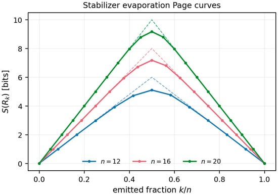
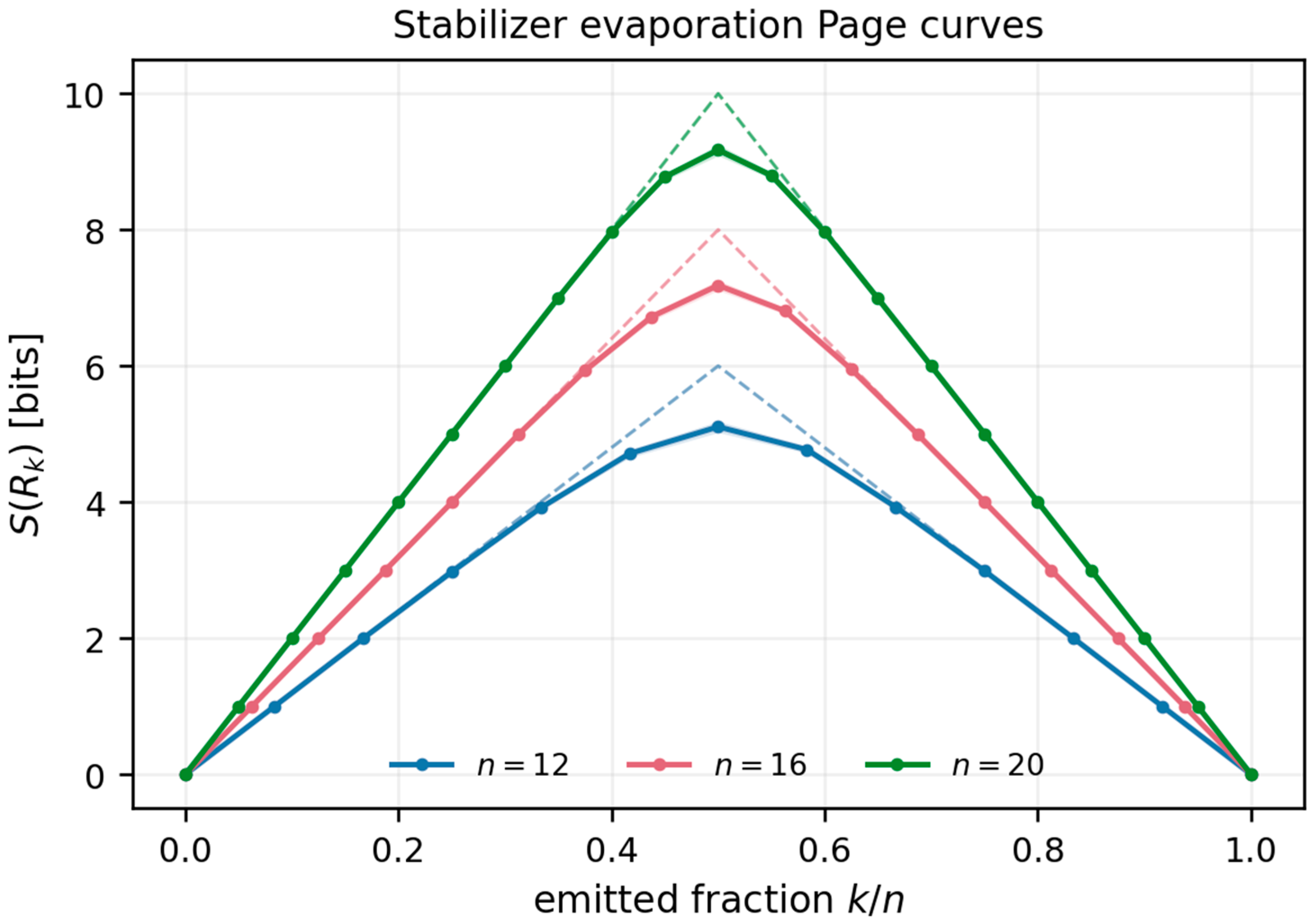
Figure 1 shows the baseline radiation entropy. The dashed lines are the maximal typical-state envelope $\mathrm{m}\mathrm{i}\mathrm{n}\left(k,n-k\right)$ bits. The simulated curves peak at $k/n=1/2$ for all three sizes but lie below the envelope near the crossing, as expected for a finite-depth Clifford ensemble rather than an independently sampled uniform state at every cut.

Figure 1. Baseline radiation entropy for the seeded stabilizer evaporation model. Points show ensemble means; shaded regions are $95\%$ normal standard-error intervals. Dashed curves show $\mathrm{m}\mathrm{i}\mathrm{n}\left(k,n-k\right)$. The entropy returns exactly to zero after complete evaporation because the baseline global state is pure.

For the main size $n=16$, the peak is $S\left(R\right)=7.184\pm 0.038$ bits (mean $\pm$ standard error), at $k/n=0.500$. This agreement with the half-emission location validates the unitary bookkeeping, but it does not by itself distinguish an island mechanism from generic finite-system unitarity.

10.2. Pairwise Network Versus Multipartite Correlation

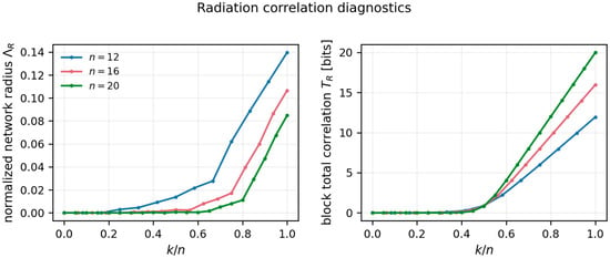
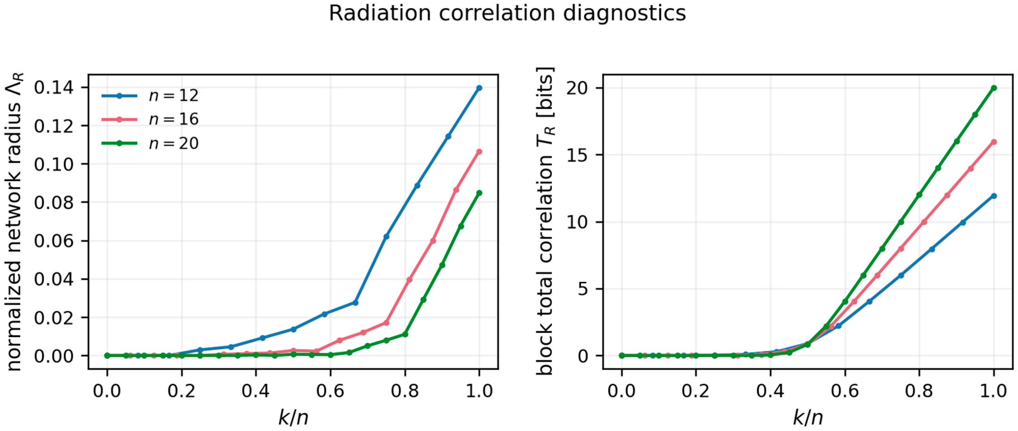
Figure 2 displays the normalized pairwise network radius and total correlation for the four-block coarse graining. They do not carry the same information. ${\Lambda }_R$ remains small through the entropy peak and rises only at later emitted fractions. By contrast, $T_R$ grows extensively as the full radiation approaches a globally pure, highly correlated stabilizer state. At $k=n$, $S\left(R\right)=0$ while individual blocks remain mixed, so $T_R=\sum _{i}S\left(R_i\right)$ can be large even when pairwise edges remain weak.

Figure 2. Radiation correlation diagnostics for a balanced partition into at most four blocks. (Left): rigorously normalized pairwise mutual-information network radius (Proposition 1). (Right): multipartite total correlation (60). Pairwise connectivity misses much of the late multipartite structure.

This result corrects a strong interpretation of the network onset. A rising pairwise spectral radius can be a useful empirical marker for a chosen partition, but its absence does not imply an absence of encoded global information. Conversely, a rise does not construct a recovery channel. The total-correlation comparison is therefore not cosmetic: it is a diagnostic for information lost by representing a many-body state as a pairwise graph.

10.3. Reference Information Transfer and Decoupling

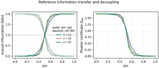
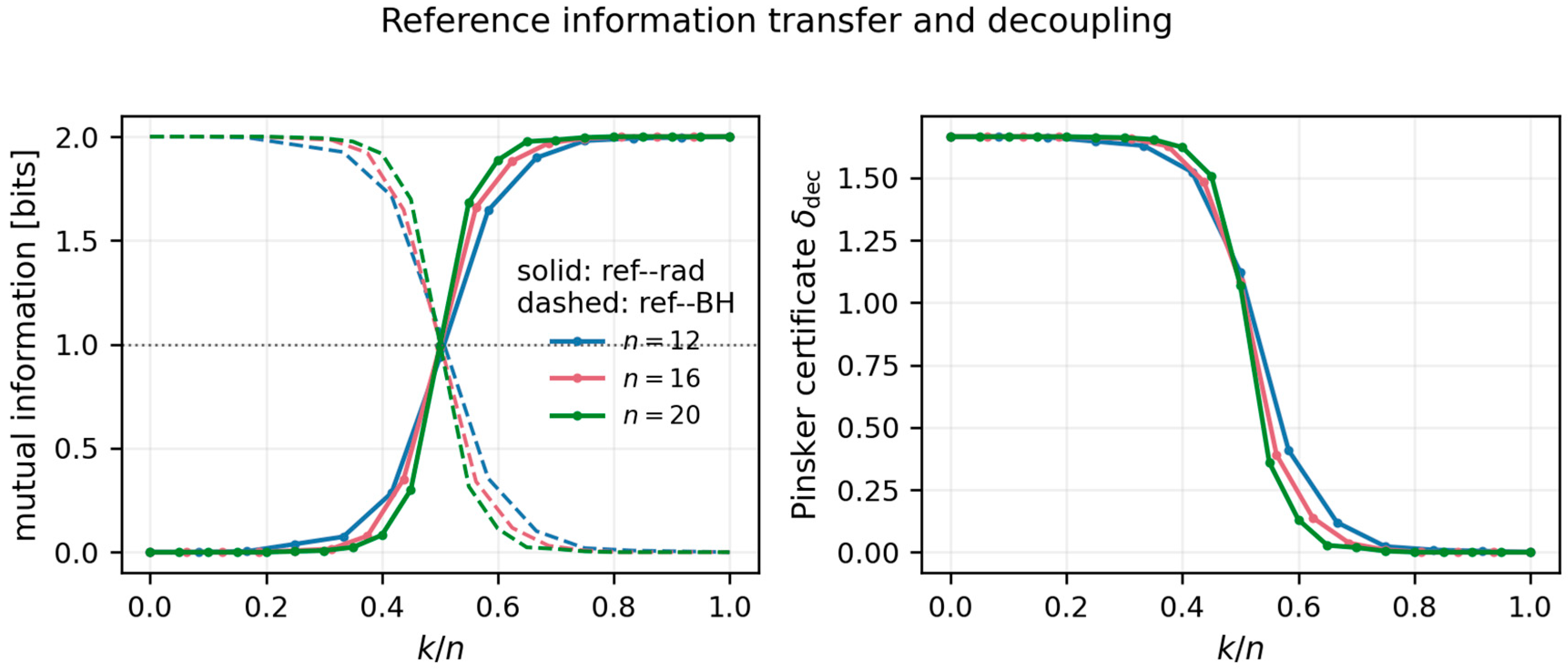
The reference ensemble directly probes a logical message. Figure 3 shows that $I\left(Q:R_k\right)$ rises from zero to two bits while $I\left(Q:B_k\right)$ falls from two to zero, with the exact sum fixed by (45). The reference midpoint occurs near half evaporation, whereas the stricter decoupling certificate becomes small later.

Figure 3. Reference information transfer. (Left): solid curves are $I\left(Q:R_k\right)$ and dashed curves are $I\left(Q:B_k\right)$; their sum is exactly two bits for every trajectory. (Right): Pinsker certificate ${\delta }_{\mathrm{d}\mathrm{e}\mathrm{c}}$ from (47). The equal-information midpoint is distinct from strong decoupling. The horizontal line in the left panel marks one bit of mutual information.

For $n=16$, the interpolated midpoint is $k/n=0.501$, while $I\left(Q:B\right)<0.1$ bit occurs at $k/n=0.637$. The separation quantifies an important conceptual point as follows: information beginning to appear in the radiation, equal sharing with the reference, and near decoupling of the erased complement are different thresholds.

10.4. Finite-Size Comparison

Table 1 and Figure 4 compare the three extracted locations.

Table 1. Transition fractions extracted from ensemble means. The entropy peak is an integer-step location; the other two entries use linear interpolation.

$\mathit{n}$	Entropy Peak $\mathit{k}/\mathit{n}$	$\mathit{I}\left(\mathit{Q}:\mathit{R}\right)=\mathbf{1}$ $\mathit{k}/\mathit{n}$	$\mathit{I}\left(\mathit{Q}:\mathit{B}\right)\mathbf{<}\mathbf{0.1}$ $\mathit{k}/\mathit{n}$
12	0.500	0.507	0.668
16	0.500	0.501	0.637
20	0.500	0.501	0.607

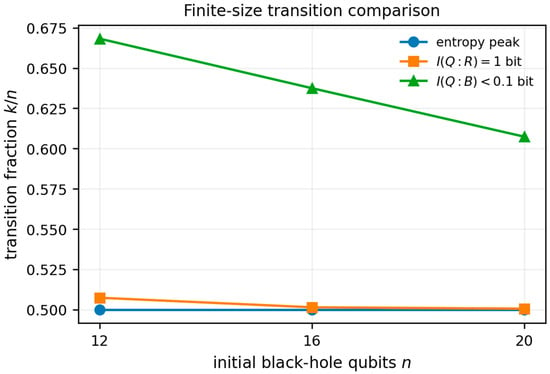
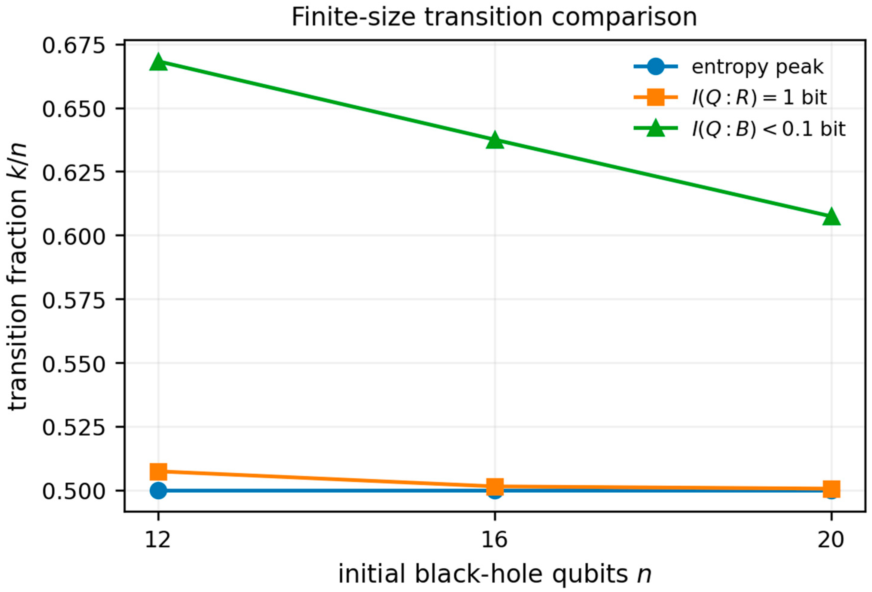
Figure 4. Finite-size comparison of the entropy peak, equal-reference-information midpoint, and stricter decoupling threshold. The three operational statements converge differently.

The entropy peak is pinned to $1/2$ by the symmetric qubit-counting setup. The reference midpoint is close to $1/2$ with finite-ensemble and discrete-step variation. The $0.1$-bit decoupling threshold remains later. With only three modest sizes, we do not fit a thermodynamic scaling law. The defensible conclusion is qualitative: midpoint transfer tracks the Page location, while a strict recovery-oriented criterion retains a finite delay in this circuit family.

11. Interpretation, Predictions, and Limitations

11.1. What Is New and What Remains Input

The framework does not offer a second derivation of the island formula. Its new content is separation and a set of operational consequences. Once a gravitational calculation supplies the QES candidate set and $\Delta S_{\mathrm{g}\mathrm{e}\mathrm{n}}$, a declared reconstruction experiment supplies $\Delta {\Phi }_{\mathrm{r}\mathrm{e}\mathrm{c}}$. The response

$$t_{\mathrm{r}\mathrm{e}\mathrm{c}}-t_{\mathrm{P}\mathrm{a}\mathrm{g}\mathrm{e}}=-\mu {\displaystyle \frac{\Delta {\Phi }_{\mathrm{r}\mathrm{e}\mathrm{c}}}{{\dot{\Delta S}}_{\mathrm{g}\mathrm{e}\mathrm{n}}}}+O\left({\mu }^2\right)$$

(78)

then predicts how an operational support threshold depends on the local steepness of the physical saddle competition. A shallow crossing amplifies task-dependent effects; a steep crossing suppresses them. This is falsifiable in models where both a QES calculation and a decoder or recovery bound are accessible.

The weights in (21) remain inputs until a task fixes them. Rather than hiding this fact, a useful application should publish a sensitivity analysis over the weights and report the features separately. A unique scalar score is meaningful only after a decision rule or resource model has been specified.

11.2. Predictions for Stronger Models

The operational score can be tested through several related predictions without being treated as gravitational entropy. The saddle-slope response predicts that, for the same recovery task across a family of semiclassical models, the displacement of the support crossing should scale inversely with $\left|{\dot{\Delta S}}_{\mathrm{g}\mathrm{e}\mathrm{n}}\right|$ when the first-order regime applies. Threshold ordering provides another test as follows: an entropy saddle exchange, an equal-reference-information point, a small-decoupling threshold, and an executable decoder-fidelity threshold need not coincide, and stronger recovery criteria should generally occur no earlier than weaker correlation criteria in a fixed dynamical family. A further diagnostic is the partition instability of pairwise networks. If a claimed reconstruction onset moves substantially under reasonable radiation blockings while a reference-decoupling diagnostic remains stable, the network onset is a coarse-graining artifact. The multipartite gap offers a complementary test because random circuits and tensor networks can exhibit large $T_R$ with small ${\Lambda }_R$, and such a gap predicts the failure of pairwise network connectivity as a stand-alone recovery proxy. Finally, complexity separation predicts that decoder gate complexity may increase even after state-recovery fidelity becomes possible, thereby distinguishing information availability from practical accessibility in a manner consistent with complexity obstructions.

11.3. Firewall Interpretation

The AMPS argument uses a late mode, its putative interior partner, and early radiation to expose a conflict among purity, semiclassical horizon smoothness, and an independent-factor description [26]. Operator-algebra reconstruction changes the bookkeeping: an interior operator represented on the radiation need not be an additional independent copy of a black-hole operator. This removes naive cloning interpretation.

It does not, by itself, prove that every state relevant to an infalling observer has a smooth horizon, nor does it erase entropic monogamy constraints. A complete resolution must specify the code subspace, gravitational dressing, state dependence if any, and the algebra accessible to each observer. The present framework contributes a precise distinction between representations and independent tensor factors; it should not be advertised as standalone proof that firewalls are absent.

11.4. Limits of the Numerical Evidence

The Clifford model has several deliberate restrictions. Stabilizer states do not reproduce generic non-Clifford complexity or the full spectrum of Haar-random reduced states. Although all-to-all random matchings model rapid mixing, they do not incorporate geometric locality, energy conservation, greybody factors, or a Hawking temperature. Relabeling qubits as radiation is unitary bookkeeping rather than a semiclassical derivation of pair creation or an island. In addition, the four-block network depends on a chronological partition and does not include an optimized decoder. The finite system sizes therefore permit a controlled comparison but not a continuum or large-entropy extrapolation.

These limitations are why the numerical result is used to compare diagnostics, not to claim a simulation of quantum gravity.

11.5. Path to a Gravitational Test

A stronger follow-up can proceed in three layers. First, compute the no-island and island $S_{\mathrm{g}\mathrm{e}\mathrm{n}}$ branches in a specific JT-gravity-plus-bath geometry, including the renormalization scheme and endpoint equations. Second, identify a finite-dimensional code or tensor-network discretization whose radiation channel admits a Petz, twirled-Petz, or optimized recovery map. Third, compute $\Delta {\Phi }_{\mathrm{r}\mathrm{e}\mathrm{c}}$ and compare the observed recovery threshold with (31). Only if the same microscopic construction produces an effective action correction should one use (53) to move a QES.

12. Conclusions

The main conclusion is a separation principle. The Page curve, interior reconstruction, and feasible decoding refer to different mathematical questions and should not be identified merely because they may occur at comparable stages of evaporation. The island/QES prescription selects the physical saddle that computes a radiation entropy. Reconstruction is instead a statement about a channel or an operator representation on a specified code subspace, with a specified norm and error tolerance. Decoder complexity asks whether that representation can be implemented with available resources. Keeping these levels distinct preserves the standard gravitational entropy calculation while still allowing operational information to be compared across its candidate saddles.

This separation leads to a concrete two-stage framework. In the first stage, the candidate set and the Page crossing are obtained solely from generalized entropy. In the second, the candidates are evaluated using a declared reconstruction-support functional that can include recovery, connectivity, algebraic, and complexity diagnostics. Near a nondegenerate Page crossing, the resulting operational transition admits the controlled expansion

$$t_{\mathrm{r}\mathrm{e}\mathrm{c}}-t_{\mathrm{P}\mathrm{a}\mathrm{g}\mathrm{e}}=-\mu {\displaystyle \frac{\Delta {\Phi }_{\mathrm{r}\mathrm{e}\mathrm{c}}\left(t_{\mathrm{P}\mathrm{a}\mathrm{g}\mathrm{e}}\right)}{{\dot{\Delta S}}_{\mathrm{g}\mathrm{e}\mathrm{n}}\left(t_{\mathrm{P}\mathrm{a}\mathrm{g}\mathrm{e}}\right)}}+O\left({\mu }^2\right),$$

(79)

with the full second-order correction given in Section 4. The formula is useful precisely because its assumptions are explicit: the competing branches must be smooth, the Page crossing must have nonzero slope, and the induced displacement must remain within the local perturbative regime. It therefore predicts a measurable sensitivity—operational thresholds are amplified near shallow saddle crossings—without promoting an arbitrary recovery score or gate count to a new term in gravitational generalized entropy.

The information-theoretic part of the analysis supplies corresponding safeguards. State recovery and operator reconstruction are formulated with type-consistent channels and code-subspace norms; recoverability is tied to conditional mutual information rather than to an unrestricted ordinary mutual-information ansatz. For network diagnostics, dimension-normalized mutual-information edges produce a spectral score bounded in $\left[0,1\right]$, making comparisons across block sizes meaningful. The comparison with multipartite total correlation also identifies a structural failure mode: pairwise connectivity can be small even when the radiation contains an extensive global constraint. Consequently, a pairwise graph may be a useful descriptive observable, but it cannot serve as a stand-alone certificate of reconstruction.

The reproducible random-Clifford evaporation experiment demonstrates why these distinctions are operationally consequential. Across $n=12,16,20$ black-hole qubits and 256 seeded realizations per size and ensemble, the radiation-entropy maximum is located at an emitted fraction close to $1/2$, and the equal-reference-information point occurs near the same location. A stricter $0.1$-bit reference-decoupling condition is reached later. At the same time, the pairwise network score and multipartite total correlation display qualitatively different behavior. Thus, even in a finite, exactly reproducible setting there is no single universal “recovery time”: its value depends on whether one asks for an entropy turnover, balanced information transfer, strong decoupling, or an executable decoder. The finite-size data do not establish a continuum scaling law, but they do provide a controlled counterexample to the assumption that these criteria must coincide.

The scope of the result is deliberately limited. The reconstruction-support functional is an operational ranking rule, not an alternative island formula; the Clifford circuit is a diagnostic toy model, not a simulation of semiclassical gravity; and the operator-algebra interpretation does not by itself prove horizon smoothness. A decisive gravitational test should combine, within one microscopic construction, a renormalized island calculation, a specified code subspace, and an explicit recovery channel such as a Petz, twirled-Petz, or optimized decoder. Computing the saddle slope, the operational score difference, and the decoder error in that common model would directly test (79). Extending the numerical study to non-Clifford dynamics, larger systems, locality and energy constraints, and bootstrap transition intervals would separately test which of the observed threshold orderings survive beyond the stabilizer setting. In this form, the present work offers neither a replacement for the island rule nor a claim that the information problem is solved; it provides a mathematically controlled interface between gravitational saddle selection and operational quantum-information recovery.

This interface also makes the proposal falsifiable in a way that a purely qualitative association between islands and decoding is not. A successful application should report the competing $S_{\mathrm{g}\mathrm{e}\mathrm{n}}$ branches and their local slope, state the code subspace and recovery norm, display the individual components and weight sensitivity of ${\Phi }_{\mathrm{r}\mathrm{e}\mathrm{c}}$, and compare the predicted transition displacement with a directly measured recovery error. It should also test whether any network diagnostic is stable under reasonable changes in radiation partition. Failure of the linear and quadratic response formulas within their declared regime, persistent disagreement between the predicted and observed threshold ordering, or strong partition dependence of the proposed support signal would count against the framework rather than being absorbed into a redefinition of entropy. Conversely, agreement across these independent checks would establish a nontrivial operational relation between island dominance and reconstruction without conflating the two. This distinction between a physical entropy saddle and an auditable recovery criterion is the central methodological result of the paper. Supporting derivations and technical details are provided in Appendix A, Appendix B, Appendix C, Appendix D, Appendix E and Appendix F.

References

- Hawking, S.W. Particle creation by black holes. Commun. Math. Phys. 1975, 43, 199–220. [Google Scholar] [CrossRef] [Scilit]
- Hawking, S.W. Breakdown of predictability in gravitational collapse. Phys. Rev. D 1976, 14, 2460–2473. [Google Scholar] [CrossRef] [Scilit]
- Page, D.N. Average entropy of a subsystem. Phys. Rev. Lett. 1993, 71, 1291–1294. [Google Scholar] [CrossRef] [Scilit] [PubMed]
- Page, D.N. Information in black hole radiation. Phys. Rev. Lett. 1993, 71, 3743–3746. [Google Scholar] [CrossRef] [Scilit] [PubMed]
- Engelhardt, N.; Wall, A.C. Quantum extremal surfaces: Holographic entanglement entropy beyond the classical regime. J. High Energy Phys. 2015, 2015, 73. [Google Scholar] [CrossRef] [Scilit]
- Almheiri, A.; Engelhardt, N.; Marolf, D.; Maxfield, H. The entropy of bulk quantum fields and the entanglement wedge of an evaporating black hole. J. High Energy Phys. 2019, 2019, 63. [Google Scholar] [CrossRef] [Scilit]
- Penington, G. Entanglement wedge reconstruction and the information paradox. J. High Energy Phys. 2020, 2020, 2. [Google Scholar] [CrossRef] [Scilit]
- Almheiri, A.; Mahajan, R.; Maldacena, J.; Zhao, Y. The Page curve of Hawking radiation from semiclassical geometry. J. High Energy Phys. 2020, 2020, 149. [Google Scholar] [CrossRef] [Scilit]
- Penington, G.; Shenker, S.H.; Stanford, D.; Yang, Z. Replica wormholes and the black hole interior. J. High Energy Phys. 2022, 2022, 205. [Google Scholar] [CrossRef] [Scilit]
- Almheiri, A.; Hartman, T.; Maldacena, J.; Shaghoulian, E.; Tajdini, A. Replica wormholes and the entropy of Hawking radiation. J. High Energy Phys. 2020, 2020, 13. [Google Scholar] [CrossRef] [Scilit]
- Almheiri, A.; Hartman, T.; Maldacena, J.; Shaghoulian, E.; Tajdini, A. The entropy of Hawking radiation. Rev. Mod. Phys. 2021, 93, 035002. [Google Scholar] [CrossRef] [Scilit]
- Bardeen, J.M.; Carter, B.; Hawking, S.W. The four laws of black hole mechanics. Commun. Math. Phys. 1973, 31, 161–170. [Google Scholar] [CrossRef] [Scilit]
- Bekenstein, J.D. Black holes and entropy. Phys. Rev. D 1973, 7, 2333–2346. [Google Scholar] [CrossRef] [Scilit]
- Almheiri, A.; Dong, X.; Harlow, D. Bulk locality and quantum error correction in AdS/CFT. J. High Energy Phys. 2015, 2015, 163. [Google Scholar] [CrossRef] [Scilit]
- Dong, X.; Harlow, D.; Wall, A.C. Reconstruction of bulk operators within the entanglement wedge in gauge-gravity duality. Phys. Rev. Lett. 2016, 117, 021601. [Google Scholar] [CrossRef] [Scilit] [PubMed]
- Harlow, D. The Ryu–Takayanagi formula from quantum error correction. Commun. Math. Phys. 2017, 354, 865–912. [Google Scholar] [CrossRef] [Scilit]
- Hayden, P.; Preskill, J. Black holes as mirrors: Quantum information in random subsystems. J. High Energy Phys. 2007, 2007, 120. [Google Scholar] [CrossRef] [Scilit]
- Harlow, D.; Hayden, P. Quantum computation vs. firewalls. J. High Energy Phys. 2013, 2013, 85. [Google Scholar] [CrossRef] [Scilit]
- Brown, A.R.; Gharibyan, H.; Penington, G.; Susskind, L. The Python’s Lunch: Geometric obstructions to decoding Hawking radiation. J. High Energy Phys. 2020, 2020, 121. [Google Scholar] [CrossRef] [Scilit]
- Kim, I.H.; Tang, E.; Preskill, J. The ghost in the radiation: Robust encodings of the black hole interior. J. High Energy Phys. 2020, 2020, 31. [Google Scholar] [CrossRef] [Scilit]
- Fawzi, O.; Renner, R. Quantum conditional mutual information and approximate Markov chains. Commun. Math. Phys. 2015, 340, 575–611. [Google Scholar] [CrossRef] [Scilit]
- Sutter, D.; Berta, M.; Tomamichel, M. Multivariate trace inequalities. Commun. Math. Phys. 2017, 352, 37–58. [Google Scholar] [CrossRef] [Scilit]
- Kretschmann, D.; Schlingemann, D.; Werner, R.F. The information-disturbance tradeoff and the continuity of Stinespring’s representation. IEEE Trans. Inf. Theory 2008, 54, 1708–1717. [Google Scholar] [CrossRef] [Scilit]
- Gottesman, D. The Heisenberg representation of quantum computers. In Proceedings of the XXII International Colloquium on Group Theoretical Methods in Physics; International Press: Cambridge, MA, USA, 1999; pp. 32–43. [Google Scholar]
- Aaronson, S.; Gottesman, D. Improved simulation of stabilizer circuits. Phys. Rev. A 2004, 70, 052328. [Google Scholar] [CrossRef] [Scilit]
- Almheiri, A.; Marolf, D.; Polchinski, J.; Sully, J. Black holes: Complementarity or firewalls? J. High Energy Phys. 2013, 2013, 62. [Google Scholar] [CrossRef] [Scilit]
Disclaimer/Publisher’s Note: The statements, opinions and data contained in all publications are solely those of the individual author(s) and contributor(s) and not of MDPI and/or the editor(s). MDPI and/or the editor(s) disclaim responsibility for any injury to people or property resulting from any ideas, methods, instructions or products referred to in the content. |
© 2026 by the author. Licensee MDPI, Basel, Switzerland. This article is an open access article distributed under the terms and conditions of the Creative Commons Attribution (CC BY) license.