Holographic Bit–Mode Balance Regularization of Wheeler–DeWitt Cosmology: Determinant Running and Inflationary Closure

Abstract

This paper develops a Holographic Bit–Mode Balance (HBMB) regularization scheme for Wheeler–DeWitt cosmology. A concrete flat-FLRW plus free-scalar clock background is first deparametrized and only then split into accessible and omitted sectors using a finite holographic capacity cutoff. In an explicit $S^2$ boundary-strip reference model, the raw geometric overlap obeys $|V_{\mathit{\ell }}^{\mathrm{raw}}{|}^2\propto {\lambda }_{\mathit{\ell }}^{-1/2}$; the normalized operator matrix element inherits the same exponent, and together with ${\lambda }_{\mathit{\ell }}\sim {\mathit{\ell }}^2$, this gives the Schur-kernel class $K_{\mathit{\ell }}\sim {\mathit{\ell }}^{-3}$, while the channel basis makes the corresponding singular-value identity and its bounded-nonuniformity robustness explicit. For the normalized uncoupled single-effective-species angular Q sector, the renormalized determinant is ${\mathsf{\Gamma }}_Q^{\mathrm{ren}}\left(L\right)={\mathsf{\Gamma }}_0-(2/3)\ln L-(31/360)L^{-2}+(1/12)L^{-3}+O\left(L^{-4}\right)$. This fixes the reference logarithmic coefficient $b_{1\mathrm{sp}}=2/3$, while the inflationary normalization also depends on an effective response coefficient $c_{\chi }$ and a cutoff–e-fold mapping coefficient $c_L$, giving ${\alpha }_{\mathrm{eff}}=(3/4)(c_{\chi }/c_L)$ at leading order. For the minimal benchmark $c_{\chi }=c_L=1$, the standard Barnes-G continuation of the exact integer determinant sum gives ${\Delta }_{\mathrm{match}}^{\left(G\right)}\simeq 0.83665$; at $N_{\ast }=55$ this yields $n_s\simeq 0.96370$ and $r\simeq 3.849\times {10}^{-3}$. The scalar tilt is weakly closure-sensitive within this plateau class, whereas the tensor amplitude remains response-normalization dependent. A full gauge-fixed gravitational determinant, microscopic response/screen-evolution laws, and a microscopic reheating mechanism remain open.

1. Introduction

Canonical quantum cosmology is naturally led to the Wheeler–DeWitt (WDW) equation

$$\widehat{\mathcal{H}}\mathsf{\Psi }[h_{ij},\mathsf{\Phi }]=0,$$

(1)

where $h_{ij}$ is the three-metric on a spatial slice, $\mathsf{\Phi }$ collectively denotes matter degrees of freedom, and $\mathsf{\Psi }[h_{ij},\mathsf{\Phi }]$ is the corresponding wave functional. This formal equation is defined on the full superspace of three-geometries and matter configurations [1,2,3,4,5,6], and well-known boundary-condition proposals for the wave function of the Universe [7,8] address which solutions are physically selected. Two longstanding problems then appear simultaneously. First, superspace contains an uncontrolled ultraviolet sector with arbitrarily many modes. Second, the WDW equation is a constraint rather than an ordinary Schrödinger equation, so standard projection and effective-Hamiltonian techniques must be used with care. At the same time, any proposed truncation principle should be positioned against the broader holographic and horizon-entropy literature [9,10,11,12], as well as thermodynamic perspectives on gravitational dynamics [13].

Direct analyses of the WDW equation have recently attracted renewed attention in holographic contexts, including semiclassical WDW states of black-hole interiors [14] and reformulations of the holographic dictionary in which deformed boundary partition functions solve the WDW equation on Cauchy slices [15]. Particularly relevant here are perturbative analyses showing that the WDW constraints intrinsically encode holographic behavior: in asymptotically AdS spacetimes, solutions of the constraints are uniquely fixed by boundary data in an infinitesimal time interval [16], while in asymptotically de Sitter spacetimes, cosmological correlators in an arbitrarily small region suffice to specify the state [17]. Those works characterize how the gravitational constraints localize information; the present construction addresses a complementary problem—the uncontrolled ultraviolet mode content of superspace—by imposing a holographic capacity bound as a regularization principle and extracting cosmological observables from the resulting projected dynamics. The fact that the constraints are intrinsically holographic in the information-theoretic sense supports, rather than competes with, the use of a holographic capacity bound as a natural regulator.

1.1. HBMB Capacity Regularization

The HBMB (Holographic Bit–Mode Balance) viewpoint suggests a concrete strategy for the ultraviolet-mode problem. In the broader HBMB program, this principle has already been developed in geometry-independent form, in a local U(1)-screen realization, and in applications to the fine-structure constant and horizon-based vacuum-energy scaling [18,19,20,21]. A local screen or horizon is assigned a finite information capacity fixed by its entropy budget,

$$C\left(R\right)\equiv S\left(R\right)={\displaystyle \frac{A\left(R\right)}{4{\mathit{\ell }}_P^2}},$$

(2)

where natural entropy units are used, $A\left(R\right)$ is the screen area, and ${\mathit{\ell }}_P$ is the Planck length. The corresponding capacity in binary bits is $C/\ln 2$.

It is useful to distinguish this information capacity from a count of basis functions. We define the total information carried by the redundancy-free accessible Hilbert space as

$$\begin{array}{|c|}\hline I_{\mathrm{acc}}^{\mathrm{tot}}\left(R\right)\equiv \ln \dim {\mathcal{H}}_{\mathrm{acc}}\left(R\right)\\ \hline\end{array}$$

(3)

and apply the holographic budget to the capacity-charged information above a fixed reference seed,

$$I_{\mathrm{acc}}^{\mathrm{cap}}\left(R\right)\equiv I_{\mathrm{acc}}^{\mathrm{tot}}\left(R\right)-I_{\mathrm{seed}},I_{\mathrm{acc}}^{\mathrm{cap}}\left(R\right)\le C\left(R\right),$$

(4)

with equality at saturation. The seed is a bookkeeping regulator already present in the reference sector and is not charged against the incremental screen budget.

For the normalized single-effective-species angular reference sector used below, the number of spherical channels up to angular multipole L is

$$N_{\mathrm{ch}}\left(L\right)={\displaystyle \sum _{\mathit{\ell }=0}^L}(2\mathit{\ell }+1)={(L+1)}^2.$$

(5)

If one redundancy-free angular channel has an effective local Hilbert-space dimension $d_{\mathrm{ch}}$, its information cost is ${\kappa }_{\mathrm{ch}}\equiv \ln d_{\mathrm{ch}}$. We parameterize the fixed seed by

$$I_{\mathrm{seed}}\equiv {\kappa }_{\mathrm{ch}}\nu ,\nu \ge 0,$$

(6)

so that

$$\begin{array}{|c|}\hline I_{\mathrm{acc}}^{\mathrm{cap}}={\kappa }_{\mathrm{ch}}\left[{(L+1)}^2-\nu \right].\\ \hline\end{array}$$

(7)

Here, $\nu$ is measured in effective channel units; it is a soft reference offset, not a literal fractional number of physical states. It is therefore convenient to measure the screen capacity in the same units,

$$N_{\mathrm{acc}}\left(R\right)\equiv {\displaystyle \frac{C\left(R\right)}{{\kappa }_{\mathrm{ch}}}}.$$

(8)

At saturation, Equations (4)–(8) then give

$$\begin{array}{|c|}\hline {(L\left(R\right)+1)}^2=N_{\mathrm{acc}}\left(R\right)+\nu .\\ \hline\end{array}$$

(9)

Thus, the relation between holographic information and angular mode count is not an identification of thermodynamic entropy with a number of harmonics; it is a coarse-grained channel representation with an explicitly separated reference-seed offset.

More generally, physical species, radial multiplicities and polarizations may contribute schematically to the capacity-charged information as

$$I_{\mathrm{acc}}^{\mathrm{cap}}=\sum _s{\kappa }_s\left[N_r^{\left(s\right)}{g}_s{(L_s+1)}^2-{\nu }_s\right],$$

(10)

where s labels a physical species or sector, ${\kappa }_s$ is its information cost per redundancy-free channel, $N_r^{\left(s\right)}$ is an effective radial multiplicity, $g_s$ counts physical polarization multiplicity after redundancy removal, $L_s$ is the corresponding angular cutoff, and ${\nu }_s$ denotes any fixed reference offset in the same effective channel units. Gauge and ghost degrees of freedom are not physical accessible screen states and therefore are not included in Equation (10); they belong instead to a fully gauge-fixed fluctuation determinant. The present paper does not construct that full determinant and restricts its explicit spectral calculation to the normalized single-effective-species angular reference sector.

In the present cosmological application HBMB is used in its weakest form: it supplies a finite capacity-controlled angular cutoff $L\left(R\right)$ on the non-clock mode content, so that the deparametrized dynamics splits into an accessible sector and an omitted high-ℓ tail whose influence can be computed rather than simply discarded. No result below depends on the stronger fixed-point applications of HBMB developed elsewhere [18,19,20,21]; the analysis therefore depends only on this capacity-regularization principle and on the explicitly stated effective closures that follow it.

1.2. Main Results and Logical Structure

The present paper develops that idea into a controlled quantum-cosmology program. Five elements are central to the construction.

• We do not apply Schur-complement logic directly to the raw Hamiltonian constraint. Instead, we first exhibit a concrete flat-FLRW plus free-scalar clock background, identify its positive deparametrized operator, and only then formulate the HBMB $P/Q$ projection. The angular determinant is subsequently introduced as a normalized single-effective-species reference sector rather than as the full gauge-fixed Einstein–matter fluctuation operator. This aligns the formalism more closely with standard projection methods [22,23] and with deparametrized quantum-cosmology constructions based on an internal scalar clock [24,25,26].
• The boundary-grazing kernel is not presented as a uniquely derived microscopic interaction. We separate an explicit $S^2$ strip-overlap model from an explicit tangential channel basis. For a one-dimensional retained coarse sector, rank-one coupling is a kinematic consequence rather than an independent HBMB prediction. The nontrivial geometric input is the raw strip-overlap envelope $|V_{\mathit{\ell }}^{\mathrm{raw}}|\sim {\mathit{\ell }}^{-1/2}$. The normalized operator matrix element $V_{\mathit{\ell }}^{\mathrm{strip}}=\mathcal{G}\left(R\right)V_{\mathit{\ell }}^{\mathrm{raw}}$ inherits the same exponent; in the uniform channel basis ${\sigma }_{\mathit{\ell }}=\left|V_{\mathit{\ell }}^{\mathrm{strip}}\right|$, and together with ${\lambda }_{\mathit{\ell }}\sim {\mathit{\ell }}^2$, this gives $K_{\mathit{\ell }}\sim {\mathit{\ell }}^{-3}$ and an $L^{-2}$ omitted-tail class. The exactly telescoping kernel is used only as a summable representative of that asymptotic class.
• We evaluate the omitted-sector determinant explicitly in the normalized uncoupled single-effective-species reference sector, including the interface term proportional to $L\ln L$ and the residual $L^{-3}$ contribution. After bulk and local cutoff-boundary renormalization, the determinant fixes $b_{1\mathrm{sp}}=2/3$. The subsequent inverse-square inflationary plateau is conditional on two separately stated effective inputs: the background-response coefficient $c_{\chi }$ and the cutoff–e-fold mapping coefficient $c_L$, giving ${\alpha }_{\mathrm{eff}}=(3/4)(c_{\chi }/c_L)$ at leading order. For the minimal benchmark $c_{\chi }=c_L=1$, finite-L matching is performed with the standard Barnes-G continuation of the exact integer determinant sum and gives ${\Delta }_{\mathrm{match}}^{\left(G\right)}\simeq 0.83665$.
• Reheating is treated only at an illustrative effective level. We formulate an HBMB-motivated adiabatic tail-decoupling source and distinguish it from a possible dynamical reservoir completion; the transfer efficiency and microscopic particle-production law remain unspecified  [27,28,29].
• We position the conditional inflationary benchmark relative to the observational plateau literature, especially Starobinsky and $\alpha$-attractor models [30,31,32,33,34,35,36]. The leading scalar tilt is weakly sensitive to the response normalization, whereas r scales directly with ${\alpha }_{\mathrm{eff}}$. The present leading CMB observables therefore do not uniquely distinguish HBMB from familiar plateau models; the distinction claimed here is the proposed origin of the plateau running, not a unique CMB signature.

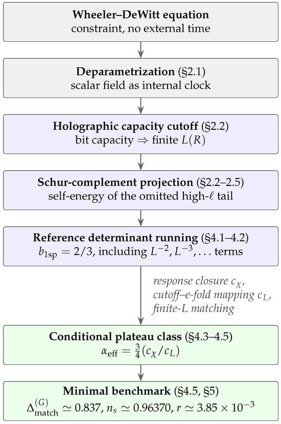
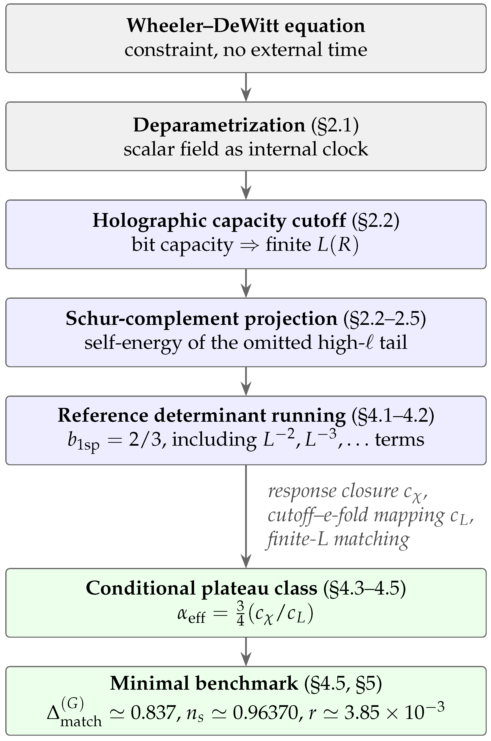
The overall picture is therefore layered. The deparametrized HBMB construction defines a finite accessible/omitted split and gives a controlled high-ℓ Schur-tail scaling in the stated angular reference sector. The renormalized uncoupled single-species determinant fixes the residual coefficient $b_{1\mathrm{sp}}=2/3$, including calculable finite-L corrections. Mapping that running to an inflationary background then requires the explicit effective quantities $c_{\chi }$ and $c_L$. The resulting inverse-square plateau class is therefore conditional, with the minimal $c_{\chi }=c_L=1$ realization providing a reproducible benchmark rather than a parameter-free HBMB prediction. This separation makes clear which results are operator/spectral calculations, which are asymptotic statements, and which depend on cosmological closure assumptions. The logical structure is summarized in Figure 1.

Figure 1. Logical structure of the construction. Gray: canonical quantum-cosmology input; purple: the HBMB regularization/reference-sector layer; green: conditional cosmological output. The deparametrized block algebra, asymptotic Schur scaling, and single-species determinant are explicit within the stated reference sector. The determinant-to-plateau step additionally requires the response coefficient $c_{\chi }$, the cutoff–e-fold mapping coefficient $c_L$, and finite-L matching; the numerical values shown in the final box refer to the minimal benchmark $c_{\chi }=c_L=1$.

2. Deparametrized WDW and the HBMB Accessible-Sector Projector

2.1. Concrete Scalar-Clock Background and Positive-Frequency Branch

A central subtlety of the WDW equation is that it is a quantum constraint rather than an ordinary spectral problem. We, therefore, make the deparametrization explicit at the homogeneous reference level before introducing the angular HBMB projection. Consider a spatially flat FLRW metric with lapse $N\left(t\right)$, scale factor $a\left(t\right)$, and a free homogeneous scalar clock $\varphi \left(t\right)$. The background action is

$$S_{\mathrm{bg}}=\int dt\left[-{\displaystyle \frac{3M_P^{2}a{\dot{a}}^2}{N}}+{\displaystyle \frac{a^3{\dot{\varphi }}^2}{2N}}\right],$$

(11)

where $M_P$ is the reduced Planck mass. The canonical momenta are

$$p_a=-{\displaystyle \frac{6M_P^{2}a\dot{a}}{N}},p_{\varphi }={\displaystyle \frac{a^3\dot{\varphi }}{N}},$$

(12)

and the Hamiltonian constraint is

$$\mathcal{C}=-{\displaystyle \frac{p_a^2}{12M_P^{2}a}}+{\displaystyle \frac{p_{\varphi }^2}{2a^3}}=0.$$

(13)

Introduce the isotropic logarithmic scale variable

$$\begin{array}{|c|}\hline x\equiv \ln (a/a_0)\\ \hline\end{array},p_x=a{p}_a,$$

(14)

with arbitrary reference scale $a_0$. Multiplying Equation (13) by $2a^3$ gives

$$p_{\varphi }^2={\displaystyle \frac{p_x^2}{6M_P^2}}.$$

(15)

For this reference minisuperspace background, we adopt the simplest Laplace-type factor ordering $p_{\varphi }\to -i{\partial }_{\varphi }$ and $p_x\to -i{\partial }_x$; alternative factor orderings are not analyzed here. This standard minisuperspace choice is discussed, for example, in refs. [3,4]. With the dimensionless scalar clock

$$\begin{array}{|c|}\hline \phi \equiv {\displaystyle \frac{\varphi }{\sqrt{6}{M}_P}}\\ \hline\end{array},$$

(16)

Equation (15) becomes

$$\begin{array}{|c|}\hline \left[{\partial }_{\phi }^2+{\Theta }_{\mathrm{bg}}\right]\mathsf{\Psi }(\phi ,x)=0,{\Theta }_{\mathrm{bg}}\equiv -{\partial }_x^2.\\ \hline\end{array}$$

(17)

For a positive $\Theta$, consistency with the positive-frequency branch requires the Klein–Gordon-type sign convention in Equation (17); the alternative form $[-{\partial }_{\phi }^2+\Theta ]\mathsf{\Psi }=0$ would not generate the oscillatory clock evolution used below.

For the reference background, we take

$${\mathcal{H}}_{\mathrm{bg}}=L^2(\mathbb{R},dx),D\left({\Theta }_{\mathrm{bg}}\right)=H^2\left(\mathbb{R}\right).$$

(18)

On this domain,

$$⟨f,{\Theta }_{\mathrm{bg}}f⟩={\int }_{\mathbb{R}}{\left|{\partial }_{x}f\right|}^{2}dx\ge 0,$$

(19)

so ${\Theta }_{\mathrm{bg}}$ is positive and self-adjoint, with spectrum $\sigma \left({\Theta }_{\mathrm{bg}}\right)=[0,\infty )$. In Fourier space, let q denote the wave number conjugate to the logarithmic minisuperspace coordinate x (not the cosmological comoving wave number used in Section 5). Writing ${\mathsf{\Psi }}_q(\phi ,x)={\psi }_q\left(\phi \right)e^{iqx}$ gives

$${\partial }_{\phi }^2{\psi }_q+q^2{\psi }_q=0;$$

(20)

so, the positive-frequency branch is explicitly

$$\begin{array}{|c|}\hline i{\partial }_{\phi }{\mathsf{\Psi }}_q=\left|q\right|{\mathsf{\Psi }}_q=\sqrt{-{\partial }_x^2}{\mathsf{\Psi }}_q.\\ \hline\end{array}$$

(21)

The positive-frequency sector therefore carries the usual $L^2$ inner product and unitary evolution generated by $\sqrt{{\Theta }_{\mathrm{bg}}}$. This concrete construction is used to establish the status of the internal clock and the positive operator to which projection methods are applied, in the same general spirit as scalar-clock deparametrizations in quantum cosmology  [24,25,26].

The homogeneous model does not by itself derive the full scalar–vector–tensor or gauge-fixed gravitational fluctuation operator. The angular calculation below is therefore stated explicitly as a normalized massless single-effective-species reference sector. A complete Einstein–matter treatment would require construction of the physical polarization sectors together with the associated gauge and ghost determinants; that extension is beyond the scope of the present work.

2.2. Accessible and Omitted Angular Sectors

For the angular reference factor, we use the standard scalar-Laplacian spectrum on the unit two-sphere, normalized here as

$${\Theta }_{\mathrm{ang}}|\mathit{\ell }m⟩={\lambda }_{\mathit{\ell }}|\mathit{\ell }m⟩,\begin{array}{|c|}\hline {\lambda }_{\mathit{\ell }}=\mathit{\ell }(\mathit{\ell }+1)\\ \hline\end{array},$$

(22)

which should be understood as the massless single-effective-species specialization used in the explicit determinant calculation, not as the complete gravitational fluctuation spectrum. Standard spherical-harmonic eigenvalue and large-order asymptotic conventions are summarized in the NIST Digital Library of Mathematical Functions (DLMF) [37].

HBMB introduces a projector onto the screen-accessible angular sector,

$$P_R=\sum _{\mathit{\ell }\le L\left(R\right)}{\displaystyle \sum _{m=-\mathit{\ell }}^{\mathit{\ell }}}|\mathit{\ell }m⟩⟨\mathit{\ell }m|,Q_R=1-P_R.$$

(23)

Thus, $P_R$ retains the angular modes that the screen capacity can represent, while $Q_R$ contains the omitted high-ℓ tail beyond the capacity bound. In the channel units of Equations (7) and (8), the saturated cutoff is therefore the relation already obtained in Equation (9). The same $\nu \ge 0$ denotes the non-capacity-charged reference-seed offset of Equation (6). The projector respects the information budget because the capacity condition is applied to ${\kappa }_{\mathrm{ch}}[{(L+1)}^2-\nu ]$, not to the seed contribution itself.

Writing $P\equiv P_R$ and $Q\equiv Q_R$, a regulated deparametrized operator has block form

$$\Theta -{\omega }^2=\left(\begin{array}{cc}A-{\omega }^2& B\\ B^{†}& D-{\omega }^2\end{array}\right),A=P\Theta P,B=P\Theta Q,D=Q\Theta Q.$$

(24)

Here, $\omega$ is the spectral parameter associated with the positive-frequency deparametrized problem; equivalently, ${\omega }^2$ is the spectral value at which the block resolvent is evaluated. The inverse ${(D-{\omega }^2)}^{-1}$ is understood on the resolvent set of D. The static reference determinant of Section 4 uses the $\omega =0$ diagonal operator $D_0$ defined below.

Eliminating the Q component gives the Feshbach–Schur effective operator [22,23],

$$\begin{array}{|c|}\hline {\Theta }_{\mathrm{eff}}\left({\omega }^2\right)=A-B{(D-{\omega }^2)}^{-1}{B}^{†}.\\ \hline\end{array}$$

(25)

The induced accessible-sector self-energy is therefore

$${\mathsf{\Sigma }}_P\left({\omega }^2\right)=-B{(D-{\omega }^2)}^{-1}{B}^{†}.$$

(26)

At a finite regulator, the associated block-determinant identity is

$$\begin{array}{|c|}\hline \det (\Theta -{\omega }^2)=\det (D-{\omega }^2)\det \left[A-{\omega }^2-B{(D-{\omega }^2)}^{-1}{B}^{†}\right].\\ \hline\end{array}$$

(27)

This identity makes explicit a distinction that will be important in Section 4. The Schur self-energy ${\mathsf{\Sigma }}_P$ is sensitive only to those linear combinations of Q that couple through B, whereas the Gaussian omitted-sector determinant

$${\mathsf{\Gamma }}_Q={\displaystyle \frac{1}{2}}{\mathrm{Tr}}_Q\ln (D-{\omega }^2)$$

(28)

traces the full regulated Q spectrum. There is therefore no contradiction between a one-dimensional retained sector coupling to one collective Q direction and the determinant carrying the full $(2\mathit{\ell }+1)$ angular degeneracy.

For the explicit determinant in Section 4, we take the diagonal reference block

$$D_0\equiv Q{\Theta }_{\mathrm{ang}}Q,$$

(29)

and treat the boundary-grazing retained–omitted mixing as a separate effective off-diagonal kernel,

$$V_{\mathrm{mix}}=P{V}_{\mathrm{mix}}Q+Q{V}_{\mathrm{mix}}P,P{V}_{\mathrm{mix}}P=Q{V}_{\mathrm{mix}}Q=0.$$

(30)

This is an effective projected construction; we do not claim that $V_{\mathrm{mix}}$ is the complete projection of a specified local microscopic Einstein–matter interaction. If a future microscopic operator also generates a nonzero diagonal term $QVQ$, that term can modify the omitted-sector determinant and, in particular, its residual logarithmic coefficient. Accordingly, the coefficient obtained in Section 4 will be denoted $b_{1\mathrm{sp}}$ and refers only to the uncoupled normalized single-effective-species reference determinant.

2.3. Explicit $S^2$ Strip-Overlap Model: Raw Geometric Scaling and Parity

A natural objection concerns the special kernel

$$K_{\mathit{\ell }}\propto {\displaystyle \frac{2\mathit{\ell }+1}{{\mathit{\ell }}^2{(\mathit{\ell }+1)}^2}}.$$

(31)

The special form of this kernel requires an independent geometric justification. We, therefore, separate the asymptotic information supplied by the geometry from the exactly summable representative used later.

Consider a thin equatorial strip on $S^2$ with angular width

$${\delta }_{\mathit{\ell }}={\displaystyle \frac{c}{\mathit{\ell }+\frac{1}{2}}},$$

(32)

where $c=O\left(1\right)$. Let the normalized boundary-grazing profile be

$$b_{\mathit{\ell }}\left(\theta \right)={\mathcal{N}}_{\mathit{\ell }}W\left({\displaystyle \frac{\theta -\pi /2}{{\delta }_{\mathit{\ell }}}}\right),$$

(33)

with W localized and ${\mathcal{N}}_{\mathit{\ell }}$ fixed by the explicit normalization ${\int }_{S^2}{\left|b_{\mathit{\ell }}\left(\mathsf{\Omega }\right)\right|}^{2}d\mathsf{\Omega }=1$. The simplest retained smooth state is the monopole $Y_{00}=1/\sqrt{4\pi }$, denoted |r⟩. We first isolate the purely geometric strip-overlap factor

$$V_{\mathit{\ell }}^{\mathrm{raw}}\equiv {\int }_{S^2}{Y}_{00}\left(\mathsf{\Omega }\right)b_{\mathit{\ell }}\left(\theta \right)Y_{\mathit{\ell }0}\left(\mathsf{\Omega }\right)d\mathsf{\Omega }.$$

(34)

Equation (34) is a normalized geometric overlap, not yet the complete matrix element of the effective operator $V_{\mathrm{mix}}$; an overall retained–omitted coupling normalization can multiply it without changing the large-ℓ power derived here. Near the equator, the standard Debye/large-degree asymptotics of the Legendre functions imply an $O\left(1\right)$ oscillatory amplitude for the normalized $Y_{\mathit{\ell }0}$ factor on the $O(1/\mathit{\ell })$ strip [37], while normalization of the shrinking strip gives $b_{\mathit{\ell }}\sim {\delta }_{\mathit{\ell }}^{-1/2}$. After $\theta =\pi /2+{\delta }_{\mathit{\ell }}y$,

$$V_{\mathit{\ell }}^{\mathrm{raw}}\sim {\delta }_{\mathit{\ell }}^{1/2}\sim {\mathit{\ell }}^{-1/2},$$

(35)

so that

$$\begin{array}{|c|}\hline |V_{\mathit{\ell }}^{\mathrm{raw}}{|}^2\sim {\mathit{\ell }}^{-1}\sim {\lambda }_{\mathit{\ell }}^{-1/2}.\\ \hline\end{array}$$

(36)

Thus, the raw geometric strip overlap alone does not produce an additional inverse power of ${\lambda }_{\mathit{\ell }}$; the Schur resolvent supplies the remaining ${\lambda }_{\mathit{\ell }}^{-1}$ factor below.

For an exactly equator-reflection-symmetric profile,

$$W(\pi -\theta )=W\left(\theta \right),$$

(37)

while $Y_{\mathit{\ell }0}(\pi -\theta )={(-1)}^{\mathit{\ell }}{Y}_{\mathit{\ell }0}\left(\theta \right)$. Consequently,

$$\begin{array}{|c|}\hline V_{\mathit{\ell }}^{\mathrm{raw}}=0\mathrm{for}\mathrm{odd}\mathit{\ell }\\ \hline\end{array}$$

(38)

in the perfectly centered symmetric strip. This is an exact parity selection rule, not a numerical artifact. A displaced strip or a reflection-asymmetric profile restores both parities. The large-ℓ envelope remains $|V_{\mathit{\ell }}^{\mathrm{raw}}|\sim {\mathit{\ell }}^{-1/2}$ for a localized strip of width $O(1/\mathit{\ell })$; parity changes the sampled subsequence and prefactor, not the asymptotic envelope.

2.4. Tangential Channel Basis and Asymptotic Schur Scaling

At fixed ℓ, the exact angular multiplicity is

$$N_t\left(\mathit{\ell }\right)=2\mathit{\ell }+1.$$

(39)

An explicit discrete tangential packet basis is obtained by a unitary discrete Fourier transform of the magnetic basis,

$$\begin{array}{|c|}\hline |\mathit{\ell },j⟩={\displaystyle \frac{1}{\sqrt{2\mathit{\ell }+1}}}{\displaystyle \sum _{m=-\mathit{\ell }}^{\mathit{\ell }}}\exp \left[-{\displaystyle \frac{2\pi ijm}{2\mathit{\ell }+1}}\right]|\mathit{\ell },m⟩,\\ \hline\end{array}$$

(40)

with $j=0,\dots ,2\mathit{\ell }$. The uniform tangential combination satisfies

$${\displaystyle \frac{1}{\sqrt{2\mathit{\ell }+1}}}{\displaystyle \sum _{j=0}^{2\mathit{\ell }}}|\mathit{\ell },j⟩=|\mathit{\ell },m=0⟩.$$

(41)

Thus, the axisymmetric geometric overlap of Equation (34) selects the uniform collective direction in this tangential basis. Multiplication by the ℓ-independent effective normalization introduced below turns that overlap into the corresponding operator matrix element without changing its large-ℓ exponent.

Define the corresponding operator matrix element by

$$V_{\mathit{\ell }}^{\mathrm{strip}}\equiv ⟨r|V_{\mathrm{mix}}|\mathit{\ell },m=0⟩,V_{\mathit{\ell }}^{\mathrm{strip}}=\mathcal{G}\left(R\right)V_{\mathit{\ell }}^{\mathrm{raw}},V_{\mathit{\ell }}^{\mathrm{strip}}\sim {\mathit{\ell }}^{-1/2}.$$

(42)

Here, $\mathcal{G}\left(R\right)$ is an ℓ-independent effective normalization over the asymptotic shell considered. Its magnitude is absorbed into the overall self-energy coefficient $\beta \left(R\right)$ below; only the ℓ-dependence is used in the channel and Schur-scaling argument. If tangential isotropy makes the individual packet amplitudes equal at leading order,

$$⟨r\left|V_{\mathrm{mix}}\right|\mathit{\ell },j⟩=g_{\mathit{\ell }},\forall j,$$

(43)

then Equations (41)–(43) imply

$$V_{\mathit{\ell }}^{\mathrm{strip}}=\sqrt{N_t}{g}_{\mathit{\ell }},\begin{array}{|c|}\hline g_{\mathit{\ell }}={\displaystyle \frac{V_{\mathit{\ell }}^{\mathrm{strip}}}{\sqrt{N_t\left(\mathit{\ell }\right)}}}.\\ \hline\end{array}$$

(44)

Since $N_t\sim \mathit{\ell }$,

$$g_{\mathit{\ell }}\sim {\mathit{\ell }}^{-1},{\left|g_{\mathit{\ell }}\right|}^2\sim {\mathit{\ell }}^{-2}.$$

(45)

For a one-dimensional retained coarse sector, $P_r=|r⟩⟨r|$, the map $P_r{V}_{\mathrm{mix}}Q$ is automatically of rank at most one. We, therefore, do not regard “rank one” itself as a nontrivial HBMB prediction. The invariant quantity of interest is the nonzero singular value of the retained-to-ℓ coupling row,

$${\sigma }_{\mathit{\ell }}^2={\displaystyle \sum _{j=0}^{2\mathit{\ell }}}{\left|g_{\mathit{\ell }j}\right|}^2.$$

(46)

For the uniform case, $g_{\mathit{\ell }j}=g_{\mathit{\ell }}$, and hence,

$${\sigma }_{\mathit{\ell }}=\sqrt{N_t}|g_{\mathit{\ell }}|=|V_{\mathit{\ell }}^{\mathrm{strip}}|\sim {\mathit{\ell }}^{-1/2}.$$

(47)

The exponent is also robust against bounded nonuniform channel weights. Write

$$g_{\mathit{\ell }j}={\overline{g}}_{\mathit{\ell }}(1+{\delta }_{\mathit{\ell }j}),{\displaystyle \frac{1}{N_t}}\sum _j{\delta }_{\mathit{\ell }j}=0,$$

(48)

where ${\overline{g}}_{\mathit{\ell }}=N_t^{-1}{\sum }_j{g}_{\mathit{\ell }j}$. The uniform overlap relation gives ${\overline{g}}_{\mathit{\ell }}\sim V_{\mathit{\ell }}^{\mathrm{strip}}/\sqrt{N_t}\sim {\mathit{\ell }}^{-1}$. If the nonuniformity is bounded in mean square,

$${\displaystyle \frac{1}{N_t}}\sum _j{|1+{\delta }_{\mathit{\ell }j}|}^2=O\left(1\right),$$

(49)

then

$${\sigma }_{\mathit{\ell }}^2=N_t{\left|{\overline{g}}_{\mathit{\ell }}\right|}^2\left[{\displaystyle \frac{1}{N_t}}\sum _j{|1+{\delta }_{\mathit{\ell }j}|}^2\right]\sim {\mathit{\ell }}^{-1}.$$

(50)

Equal channel weights are therefore sufficient but not necessary for the asymptotic exponent; bounded nonuniformity can change the coefficient without changing the leading power.

Resolving Equation (26) in an omitted angular eigensector gives, schematically,

$${\mathsf{\Sigma }}_{\mathit{\ell }}\left(\omega \right)\sim -{\displaystyle \frac{{\sigma }_{\mathit{\ell }}^2}{{\lambda }_{\mathit{\ell }}-{\omega }^2}}.$$

(51)

For $\mathit{\ell }\gg 1$ at fixed $\omega$,

$$K_{\mathit{\ell }}^{\mathrm{asym}}\left(R\right)\equiv \left|{\mathsf{\Sigma }}_{\mathit{\ell }}\right|\sim {\displaystyle \frac{{\sigma }_{\mathit{\ell }}^2}{{\lambda }_{\mathit{\ell }}}}\sim {\mathit{\ell }}^{-3},\begin{array}{|c|}\hline {\displaystyle \sum _{\mathit{\ell }>L}}{K}_{\mathit{\ell }}^{\mathrm{asym}}\sim L^{-2}.\\ \hline\end{array}$$

(52)

The nontrivial geometric input of the strip/channel construction is the large-ℓ overlap envelope; combined with the angular Laplace spectrum, it implies the $K_{\mathit{\ell }}\sim {\mathit{\ell }}^{-3}$ kernel and $L^{-2}$ omitted-tail scaling. Appendix A tests the centered-strip parity rule, a displaced strip, the DFT basis, and the large-ℓ envelope numerically.

2.5. An Exactly Summable Representative Kernel

To obtain a closed-form toy realization of the asymptotic class (52), we choose the representative kernel

$$\begin{array}{|c|}\hline K_{\mathit{\ell }}\left(R\right)=\beta \left(R\right){\displaystyle \frac{2\mathit{\ell }+1}{{\mathit{\ell }}^2{(\mathit{\ell }+1)}^2}},\\ \hline\end{array}$$

(53)

where $\beta \left(R\right)$ is the overall R-dependent quadratic self-energy strength: it collects the squared retained–omitted mixing amplitude and the normalization factors that are independent of the explicit angular kernel shown in Equation (53). The term “quadratic” refers to the second-order structure $V_{PQ}{(Q\Theta Q-{\omega }^2)}^{-1}{V}_{QP}$ of Equation (26); $\beta$ is not introduced as a new fundamental coupling constant.

Using

$${\displaystyle \frac{2\mathit{\ell }+1}{{\mathit{\ell }}^2{(\mathit{\ell }+1)}^2}}={\displaystyle \frac{1}{{\mathit{\ell }}^2}}-{\displaystyle \frac{1}{{(\mathit{\ell }+1)}^2}},$$

(54)

the representative sum telescopes exactly,

$${\displaystyle \sum _{\mathit{\ell }=L+1}^{\infty }}{\displaystyle \frac{2\mathit{\ell }+1}{{\mathit{\ell }}^2{(\mathit{\ell }+1)}^2}}={\displaystyle \frac{1}{{(L+1)}^2}}.$$

(55)

We denote by $\Delta U_{\mathrm{HBMB}}\left(R\right)$ the positive magnitude of this induced tail correction when it is represented as an effective contribution to the reduced minisuperspace potential. Then,

$$\begin{array}{|c|}\hline \Delta U_{\mathrm{HBMB}}\left(R\right)={\displaystyle \frac{\beta \left(R\right)}{{(L\left(R\right)+1)}^2}}={\displaystyle \frac{\beta \left(R\right)}{N_{\mathrm{acc}}\left(R\right)+\nu }}.\\ \hline\end{array}$$

(56)

Equation (56) is therefore the exactly summable representative of the Schur asymptotic class (52); it is not a claim that the microscopic kernel is uniquely fixed to Equation  (53).

As the accessible capacity grows, the retained and omitted sectors should decouple progressively. Writing $V_{PQ}\left(R\right)$ for the capacity-dependent effective off-diagonal mixing amplitude, a minimal phenomenological implementation is

$$V_{PQ}\left(R\right)\to {\displaystyle \frac{V_{PQ}^{\left(0\right)}\left(R\right)}{\sqrt{1+N_{\mathrm{acc}}\left(R\right)/N_c}}},$$

(57)

where $V_{PQ}^{\left(0\right)}\left(R\right)$ is the baseline effective mixing before capacity suppression, and $N_c$ is a crossover capacity. Since the Schur self-energy is quadratic in the mixing, this gives

$$\begin{array}{|c|}\hline \beta \left(R\right)={\displaystyle \frac{{\beta }_0}{1+N_{\mathrm{acc}}\left(R\right)/N_c}}.\\ \hline\end{array}$$

(58)

Here, ${\beta }_0>0$ denotes the unsuppressed self-energy normalization associated with the baseline mixing amplitude $V_{PQ}^{\left(0\right)}$ before the phenomenological capacity-suppression factor is applied. The corresponding projected correction is

$$\begin{array}{|c|}\hline \Delta U_{\mathrm{HBMB}}\left(R\right)={\displaystyle \frac{{\beta }_0}{[N_{\mathrm{acc}}\left(R\right)+\nu ][1+N_{\mathrm{acc}}\left(R\right)/N_c]}}.\\ \hline\end{array}$$

(59)

This capacity-suppression factor is an illustrative effective closure rather than a microscopic derivation of the R dependence of $P\Theta Q$.

A final sign distinction is important. If $D-{\omega }^2$ is positive, the operator-level Schur correction ${\mathsf{\Sigma }}_P=-B{(D-{\omega }^2)}^{-1}{B}^{†}$ is negative semidefinite. In Equations (56)–(59), $\Delta U_{\mathrm{HBMB}}$ denotes the positive magnitude assigned to the corresponding reduced potential contribution. The relation between the operator sign and the effective minisuperspace-potential sign depends on the indefinite superspace kinetic form and on the convention used in the deparametrized operator. Only the magnitude and capacity scaling are used in the illustrative Section 3 closure.

3. Illustrative Minisuperspace Effective-Fluid Closure

3.1. Accessible Capacity Along a Dimensionless Scale-Factor Variable

To avoid confusion with the logarithmic variable $x=\ln (a/a_0)$ used in the scalar-clock background of Section 2.1, we denote the dimensionless scale factor in this illustrative minisuperspace closure by

$$\begin{array}{|c|}\hline \overline{a}\equiv {\displaystyle \frac{a}{a_0}}.\\ \hline\end{array}$$

(60)

The following capacity profile is adopted only as a simple reduced benchmark,

$$N_{\mathrm{acc}}\left(\overline{a}\right)=\pi {\overline{a}}^{2}F\left(\overline{a}\right),F\left(\overline{a}\right)={\displaystyle \frac{{\overline{a}}^2}{{\overline{a}}^2+a_F^2}},$$

(61)

where $F\left(\overline{a}\right)$ is an accessibility fraction, and $a_F$ sets the crossover between the suppressed and fully accessible regimes. The $\pi {\overline{a}}^2$ prefactor represents area-like growth of the screen capacity, consistent with Equation (2); the rational interpolation itself is illustrative and is not derived from the microscopic screen dynamics. Equivalently,

$$N_{\mathrm{acc}}\left(\overline{a}\right)=\pi {\displaystyle \frac{{\overline{a}}^4}{{\overline{a}}^2+a_F^2}}.$$

(62)

Hence,

$${\displaystyle \frac{d\ln N_{\mathrm{acc}}}{d\ln \overline{a}}}=4-{\displaystyle \frac{2{\overline{a}}^2}{{\overline{a}}^2+a_F^2}}.$$

(63)

The Schur calculation of Section 2 gives an induced potential correction $\Delta U_{\mathrm{HBMB}}$; it does not by itself identify that quantity with a cosmological energy density. To construct the present illustrative background, we therefore make an explicit effective-fluid identification

$$\begin{array}{|c|}\hline {\rho }_{\mathrm{HBMB}}^{\mathrm{eff}}\left(\overline{a}\right)\equiv C_{\rho }\Delta U_{\mathrm{HBMB}}\left(\overline{a}\right),\\ \hline\end{array}$$

(64)

where $C_{\rho }>0$ is an overall conversion factor that drops out of the equation-of-state derivative below. This is the closure step connecting the projected potential correction to the reduced FLRW fluid description; it is not an algebraic consequence of the Schur complement alone.

For the unsuppressed representative tail of Equation (56), Equation (64) gives the minimal effective-fluid profile

$${\rho }_{\mathrm{HBMB},\min }^{\mathrm{eff}}\left(\overline{a}\right)\propto {\displaystyle \frac{1}{N_{\mathrm{acc}}\left(\overline{a}\right)+\nu }}.$$

(65)

If this effective component is treated as separately conserved in the illustrative reduced background, the standard continuity relation

$${\displaystyle \frac{d\ln \rho }{d\ln a}}=-3(1+w)$$

(66)

can be written identically with $\ln \overline{a}$ because $\overline{a}=a/a_0$. Therefore,

$$w_{\min }\left(\overline{a}\right)=-1+{\displaystyle \frac{1}{3}}{\displaystyle \frac{N_{\mathrm{acc}}}{N_{\mathrm{acc}}+\nu }}{\displaystyle \frac{d\ln N_{\mathrm{acc}}}{d\ln \overline{a}}}.$$

(67)

Including the phenomenological capacity suppression of the mixing, Equation (59), gives instead

$${\rho }_{\mathrm{HBMB},\mathrm{exit}}^{\mathrm{eff}}\left(\overline{a}\right)\propto {\displaystyle \frac{1}{[N_{\mathrm{acc}}\left(\overline{a}\right)+\nu ][1+N_{\mathrm{acc}}\left(\overline{a}\right)/N_c]}}.$$

(68)

Taking the logarithmic derivative yields

$$\begin{array}{|c|}\hline w\left(\overline{a}\right)=-1+{\displaystyle \frac{1}{3}}{\displaystyle \frac{d\ln N_{\mathrm{acc}}}{d\ln \overline{a}}}\left[{\displaystyle \frac{N_{\mathrm{acc}}}{N_{\mathrm{acc}}+\nu }}+{\displaystyle \frac{N_{\mathrm{acc}}}{N_{\mathrm{acc}}+N_c}}\right].\\ \hline\end{array}$$

(69)

For a flat FLRW background dominated by this effective component, the first Hubble-flow parameter is

$$\begin{array}{|c|}\hline {ϵ}_1\left(\overline{a}\right)\equiv -{\displaystyle \frac{\dot{H}}{H^2}}={\displaystyle \frac{3}{2}}\left[1+w\left(\overline{a}\right)\right].\\ \hline\end{array}$$

(70)

Here, $H\equiv \dot{a}/a$ is the Hubble parameter. Thus, the notation used here is the same ${ϵ}_1$ employed in the inflationary analysis of Section 4 and Section 5; the present subsection is only an illustrative reduced-background realization of that standard Hubble-flow quantity.

3.2. Minimal Benchmark and Physical Meaning

For the illustrative parameters

$$\nu =0.2,a_F=0.7,N_c=3,$$

(71)

these values are chosen solely to illustrate a smooth quasi-de Sitter-to-exit transition in the reduced closure; they are not fitted parameters or independently derived microscopic constants. The reduced model exhibits a transition from an early quasi-de Sitter regime to the end of accelerated expansion at

$${\overline{a}}_{\mathrm{end}}\simeq 0.473177,$$

(72)

where $w\left({\overline{a}}_{\mathrm{end}}\right)=-1/3$, and ${ϵ}_1\left({\overline{a}}_{\mathrm{end}}\right)=1$. Selected values are shown in Table 1.

Table 1. Illustrative reduced HBMB effective-fluid benchmark for Equation (69).

$\overline{\mathit{a}}$	$\mathit{w}\left(\overline{\mathit{a}}\right)$	${\mathit{ϵ}}_1\left(\overline{\mathit{a}}\right)$
0.05	$-0.99971727$	$4.2410\times {10}^{-4}$
0.10	$-0.99558968$	$6.6155\times {10}^{-3}$
0.20	$-0.93787010$	$9.3195\times {10}^{-2}$
0.30	$-0.76101105$	$3.5848\times {10}^{-1}$
0.40	$-0.50680462$	$7.3979\times {10}^{-1}$
$0.473177$	$-0.33333329$	$1.00000006$
1.00	$0.17479975$	$1.76219963$

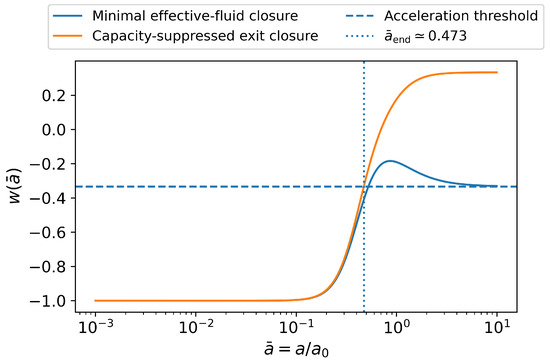
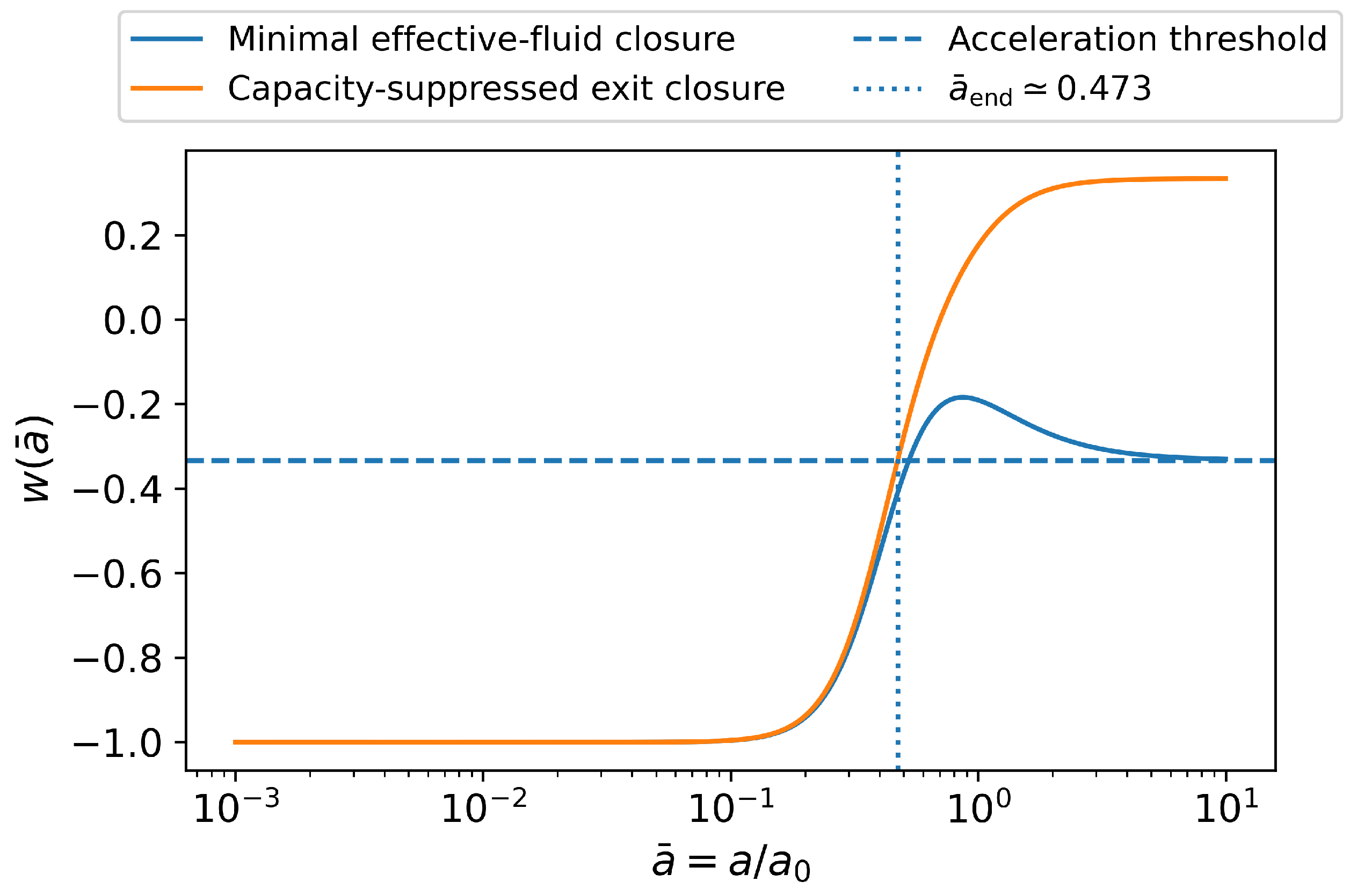
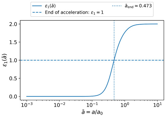
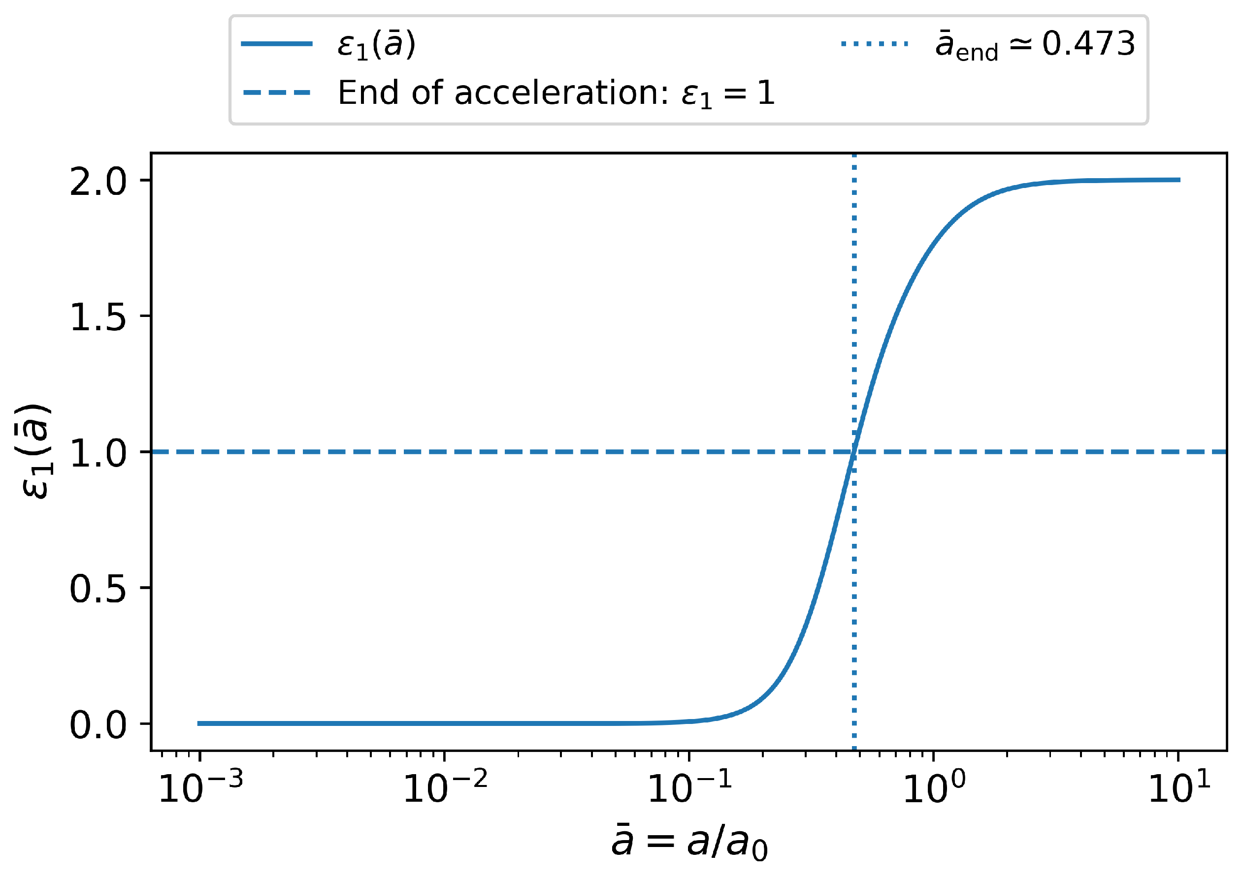
The corresponding equation-of-state and first Hubble-flow histories are shown in Figure 2 and Figure 3.

Figure 2. Equation-of-state evolution in the illustrative reduced effective-fluid closure. The minimal curve uses Equation (65); the exit curve additionally includes the phenomenological capacity suppression of Equation (68). The horizontal dashed line marks the acceleration threshold $w=-1/3$, and the vertical dotted line marks ${\overline{a}}_{\mathrm{end}}\simeq 0.473$.

Figure 3. First Hubble-flow parameter ${ϵ}_1\left(\overline{a}\right)$ for the illustrative exit closure. The horizontal line marks ${ϵ}_1=1$, and the vertical line marks the corresponding end of accelerated expansion.

The status of this section is deliberately limited. Equations (64)–(70) show how the projected tail can be represented by a simple effective fluid and how a phenomenological suppression of retained–omitted mixing can produce an exit from acceleration. They do not constitute a microscopic derivation of the energy-transfer law or a prediction of the final 50–60 e-fold inflationary trajectory. The CMB-window analysis instead uses the separately stated renormalized response closure of Section 4.

4. From the Renormalized Omitted-Sector Determinant to a Conditional Plateau Closure

4.1. Single-Species Determinant and Large-L Expansion

The central technical input of this section is the Gaussian determinant of the uncoupled normalized single-effective-species angular Q sector introduced in Section 2. It should not be identified with the determinant of the full gauge-fixed Einstein–matter fluctuation operator. The use of spectral log determinants and the separation of local ultraviolet-sensitive terms from residual spectral contributions are standard tools in one-loop, heat-kernel, and functional-determinant analyses [38,39,40,41]; the specific subtraction convention and HBMB interpretation adopted below remain part of the present reference construction. In the reference sector,

$${\mathsf{\Gamma }}_Q(L;\mathsf{\Lambda })={\displaystyle \frac{1}{2}}{\displaystyle \sum _{\mathit{\ell }=L+1}^{\mathsf{\Lambda }}}(2\mathit{\ell }+1)\ln \left[\mathit{\ell }(\mathit{\ell }+1)\right],$$

(73)

where L retains its meaning as the HBMB accessible angular cutoff, $\mathsf{\Lambda }$ is an auxiliary ultraviolet regulator, and the full $(2\mathit{\ell }+1)$ degeneracy of the reference species is retained. Additional physical polarizations, matter species, gauge sectors, ghosts, or diagonal Q-sector corrections generated by a microscopic interaction would modify the full determinant and can renormalize the residual logarithmic coefficient. Accordingly, the coefficient obtained below will be denoted $b_{1\mathrm{sp}}$.

Define

$$S\left(L\right)={\displaystyle \sum _{\mathit{\ell }=1}^L}(2\mathit{\ell }+1)\ln \left[\mathit{\ell }(\mathit{\ell }+1)\right],$$

(74)

so that ${\mathsf{\Gamma }}_Q(L;\mathsf{\Lambda })=\frac{1}{2}[S\left(\mathsf{\Lambda }\right)-S\left(L\right)]$. For integer L, the sum can be rearranged exactly as

$$S\left(L\right)=4{\displaystyle \sum _{n=1}^L}n\ln n+(2L+1)\ln (L+1)=4\ln H_L+(2L+1)\ln (L+1),$$

(75)

where $H_L={\prod }_{n=1}^L{n}^n$ is the hyperfactorial. Re-expanding the exact expression gives

$$\begin{array}{|c|}\hline \begin{array}{c}\hfill S\left(L\right)=2L^2\ln L-L^2+4L\ln L+{\displaystyle \frac{4}{3}}\ln L+C_A\\ \hfill +{\displaystyle \frac{31}{180L^2}}-{\displaystyle \frac{1}{6L^3}}+{\displaystyle \frac{47}{315L^4}}+O\left(L^{-5}\right),\end{array}\\ \hline\end{array}$$

(76)

with

$$C_A=2+4\ln A_G,$$

(77)

where $A_G$ is the Glaisher–Kinkelin constant.

The $L^{-3}$ term in Equation (76) is numerically relevant for finite-L matching. Appendix B checks the expansion directly against the exact integer sum and quantifies why a short asymptotic truncation should not be used as a precision matching formula near $L\simeq 2.3$.

4.2. Renormalized Residual Running and Response Status

The large-L structure in Equation (76) contains a bulk area-like term $2L^2\ln L-L^2$, a local interface term $4L\ln L$, and a residual logarithmic plus inverse-power contribution. After absorbing the first two pieces into the coarse background and local cutoff-boundary counterterms, the single-species residual determinant is

$$\begin{array}{|c|}\hline {\mathsf{\Gamma }}_Q^{\mathrm{ren}}\left(L\right)={\mathsf{\Gamma }}_0-{\displaystyle \frac{2}{3}}\ln L-{\displaystyle \frac{31}{360L^2}}+{\displaystyle \frac{1}{12L^3}}-{\displaystyle \frac{47}{630L^4}}+O\left(L^{-5}\right).\\ \hline\end{array}$$

(78)

Here, ${\mathsf{\Gamma }}_0$ is the L-independent finite renormalized constant left after the stated subtraction convention. It is convenient to define the positive residual running variable by

$${\mathsf{\Gamma }}_Q^{\mathrm{ren}}\left(L\right)={\mathsf{\Gamma }}_0-g_{1\mathrm{sp}}\left(L\right),$$

(79)

so that

$$\begin{array}{|c|}\hline g_{1\mathrm{sp}}\left(L\right)=b_{1\mathrm{sp}}\ln L+{\displaystyle \frac{31}{360L^2}}-{\displaystyle \frac{1}{12L^3}}+{\displaystyle \frac{47}{630L^4}}+O\left(L^{-5}\right),b_{1\mathrm{sp}}={\displaystyle \frac{2}{3}}.\\ \hline\end{array}$$

(80)

The notation $b_{1\mathrm{sp}}$ emphasizes that $2/3$ is the coefficient of the normalized uncoupled one-species reference determinant, not a universal coefficient already computed for the complete gravitational fluctuation spectrum. Schematically, a full gauge-fixed multi-sector calculation would instead produce a coefficient of the form $b_{\mathrm{eff}}={\sum }_A{\eta }_A{d}_A{b}_A$, where A labels a fluctuation sector, $d_A$ is its multiplicity, $b_A$ its residual logarithmic coefficient, and ${\eta }_A$ denotes the corresponding bosonic/ghost sign or statistical weight.

The determinant calculation fixes the running in Equation (80); it does not by itself fix how that running changes the cosmological background. We therefore introduce

$$g_{\mathrm{eff}}^{-1}\left(L\right)=g_R^{-1}+g_{1\mathrm{sp}}\left(L\right),$$

(81)

where $g_R^{-1}$ is the finite renormalized offset fixed by the chosen subtraction/reference convention. We then treat the relation

$$\begin{array}{|c|}\hline {\rho }_{\mathrm{HBMB}}\left(L\right)={\rho }_{\infty }\exp \left[-{\displaystyle \frac{c_{\chi }}{g_{\mathrm{eff}}^{-1}\left(L\right)}}\right]\\ \hline\end{array}$$

(82)

as an effective response closure. Here, $c_{\chi }$ is a dimensionless response coefficient that is not microscopically fixed in the present work, while ${\rho }_{\infty }$ is the asymptotic energy-density normalization approached when the inverse response variable becomes large. Using the Friedmann relation $H^2=\rho /\left(3M_P^2\right)$ gives

$$\begin{array}{|c|}\hline \ln H\left(L\right)=\ln H_{\infty }-{\displaystyle \frac{c_{\chi }}{2g_{\mathrm{eff}}^{-1}\left(L\right)}},H_{\infty }\equiv \sqrt{{\displaystyle \frac{{\rho }_{\infty }}{3M_P^2}}}.\\ \hline\end{array}$$

(83)

Equivalently, defining $g_{\mathrm{eff}}\equiv {\left[g_{\mathrm{eff}}^{-1}\right]}^{-1}$, Equations (82) and (83) can be written as

$$\ln \left({\displaystyle \frac{{\rho }_{\mathrm{HBMB}}}{{\rho }_{\infty }}}\right)=-c_{\chi }{g}_{\mathrm{eff}},\ln \left({\displaystyle \frac{H}{H_{\infty }}}\right)=-{\displaystyle \frac{c_{\chi }}{2}}{g}_{\mathrm{eff}}.$$

Thus, the assumed response is linear in the effective running variable at the level of the logarithm of the background density. The exponential form provides a positive completion of this phenomenological log-response; no microscopic derivation of this functional form is claimed here. The controlled determinant result and the cosmological response assumption are therefore kept as distinct logical steps.

4.3. Effective Mapping to Remaining e-Folds

A second independent input is required to map the HBMB angular cutoff to the inflationary background trajectory. We define the backward remaining-e-fold variable by

$$\begin{array}{|c|}\hline N_{\mathrm{rem}}\equiv \ln \left({\displaystyle \frac{a_{\mathrm{end}}}{a}}\right),{\displaystyle \frac{d{N}_{\mathrm{rem}}}{dt}}=-H.\\ \hline\end{array}$$

(84)

Thus, $N_{\mathrm{rem}}$ decreases toward zero at the end of inflation. Throughout the manuscript, L continues to denote the same capacity-controlled HBMB cutoff introduced in Section 2. What is not derived here is the physical screen trajectory $R\left(N_{\mathrm{rem}}\right)$ and, hence, the function $L\left[N_{\mathrm{rem}}\right]$. We therefore retain the logarithmic mapping coefficient explicitly,

$$\begin{array}{|c|}\hline {\displaystyle \frac{d\ln L}{d{N}_{\mathrm{rem}}}}=c_L,\\ \hline\end{array}$$

(85)

where $c_L$ is an effective model parameter. For a constant $c_L$ over the CMB window,

$$\begin{array}{|c|}\hline \ln {\displaystyle \frac{L}{L_0}}=c_L\left(N_{\mathrm{rem}}+\Delta \right).\\ \hline\end{array}$$

(86)

Here $L_0$ is a reference cutoff scale associated with the finite-renormalization convention, while $\Delta$ is the integration/matching shift that locates the endpoint relative to that reference scale. In the minimal benchmark below, we set $L_0=1$ and determine the finite-flow value of $\Delta$ from the end condition. The unit value $c_L=1$ used below is therefore a minimal benchmark, not a consequence of the entropy–area law alone.

For comparison only, a distinct angular scale associated with a fixed comoving wavenumber on a Hubble-sized screen would satisfy $L_{\mathrm{com}}\propto k/\left(aH\right)$. Thus, $\ln L_{\mathrm{com}}=\mathrm{const}-\ln a-\ln H$; using $d\ln a/d{N}_{\mathrm{rem}}=-1$ from Equation (84) and $d\ln H/d{N}_{\mathrm{rem}}={ϵ}_1$ gives $d\ln L_{\mathrm{com}}/d{N}_{\mathrm{rem}}=1-{ϵ}_1$. This shows that a coefficient close to unity is geometrically natural in the slow-roll regime, but we do not identify that comoving scale with the HBMB capacity cutoff entering Equation (73).

Define

$$u\equiv N_{\mathrm{rem}}+\Delta .$$

(87)

At large L,

$$g_{\mathrm{eff}}^{-1}\simeq b_{1\mathrm{sp}}{c}_{L}u$$

(88)

for the benchmark finite-renormalization choice $g_R^{-1}=0$ and $L_0=1$. Differentiating Equation (83) yields

$${ϵ}_1\equiv {\displaystyle \frac{d\ln H}{d{N}_{\mathrm{rem}}}}={\displaystyle \frac{c_{\chi }}{2}}{\displaystyle \frac{d{g}_{\mathrm{eff}}^{-1}/d{N}_{\mathrm{rem}}}{{\left(g_{\mathrm{eff}}^{-1}\right)}^2}}.$$

(89)

Using Equation (85), the leading large-L behavior becomes

$$\begin{array}{|c|}\hline {ϵ}_1\left(N_{\mathrm{rem}}\right)\simeq {\displaystyle \frac{{\alpha }_{\mathrm{eff}}}{{(N_{\mathrm{rem}}+\Delta )}^2}},{\alpha }_{\mathrm{eff}}\equiv {\displaystyle \frac{c_{\chi }}{2b_{1\mathrm{sp}}{c}_L}}.\\ \hline\end{array}$$

(90)

For the one-species coefficient $b_{1\mathrm{sp}}=2/3$,

$$\begin{array}{|c|}\hline {\alpha }_{\mathrm{eff}}={\displaystyle \frac{3}{4}}{\displaystyle \frac{c_{\chi }}{c_L}}.\\ \hline\end{array}$$

(91)

Consequently, the determinant fixes $b_{1\mathrm{sp}}$; together with the adopted response and scale-mapping closures, this running produces the inverse-square plateau class. The numerical coefficient ${\alpha }_{\mathrm{eff}}$ depends on those closures, and the value ${\alpha }_{\mathrm{eff}}=3/4$ is obtained only in the minimal benchmark $c_{\chi }=c_L=1$.

The ratio $c_{\chi }/c_L$ controls the leading asymptotic coefficient, but the two parameters are not exactly degenerate at finite L: inverse-power terms depend on $L=L_0\exp \left[c_{L}u\right]$ and therefore retain a separate $c_L$ dependence. We do not infer $c_{\chi }/c_L\simeq 1$ from current observations; constraining that combination would require a dedicated likelihood analysis.

4.4. Finite-L Matching: ${\Delta }_{\mathrm{asy}}$ Versus ${\Delta }_{\mathrm{match}}^{\left(G\right)}$

The large-L plateau approximation and the finite-L end matching should not be conflated. If Equation  (90) is extrapolated by itself to $N_{\mathrm{rem}}=0$, its own end condition gives

$$1={\displaystyle \frac{{\alpha }_{\mathrm{eff}}}{{\Delta }_{\mathrm{asy}}^2}}⟹\begin{array}{|c|}\hline {\Delta }_{\mathrm{asy}}=\sqrt{{\alpha }_{\mathrm{eff}}}.\\ \hline\end{array}$$

(92)

For the minimal benchmark, this is ${\Delta }_{\mathrm{asy}}=\sqrt{3}/2\simeq 0.8660254$.

However, the end of inflation lies at $L=O\left(1\right)$ in the reference convention and is not an asymptotic regime. We, therefore, use the standard Barnes-G analytic continuation of the exact integer identity in Equation (75) for finite-L matching. The Barnes function is defined by $G\left(1\right)=1$ and $G(z+1)=\mathsf{\Gamma }\left(z\right)G\left(z\right)$; standard properties are summarized in DLMF [37]. Using

$$H_L={\displaystyle \frac{\mathsf{\Gamma }{(L+1)}^L}{G(L+1)}},$$

(93)

we define

$$\begin{array}{|c|}\hline S_G\left(L\right)=4\left[L\ln \mathsf{\Gamma }(L+1)-\ln G(L+1)\right]+(2L+1)\ln (L+1), \\ \hline\end{array}$$

(94)

which exactly reproduces Equation (75) at integer L and provides its standard smooth continuation between integers. At integer L, the construction coincides with the literal spectral projector of Section 2; between integers, L is used only as a smooth effective running coordinate for the coarse-grained response and finite-L interpolation. We stress that this is an analytic continuation of the exact integer partial sum, not a new scheme-independent definition of a fundamental noninteger determinant.

In the benchmark convention $g_R^{-1}=0$, $L_0=1$, define

$$g_G\left(L\right)={\displaystyle \frac{1}{2}}\left[S_G\left(L\right)-\left(2L^2\ln L-L^2+4L\ln L\right)-C_A\right]$$

(95)

The function $g_G\left(L\right)$ is the Barnes-G finite-L continuation of the same residual running represented asymptotically by $g_{1\mathrm{sp}}\left(L\right)$ in Equation (80). Thus, $g_G\left(L\right)$ is used for endpoint interpolation, while Equation (80) displays the controlled large-L expansion. We also define

$$D_G\left(L\right)\equiv {\displaystyle \frac{d{g}_G}{d\ln L}}.$$

(96)

By the chain rule and Equation (85),

$${\displaystyle \frac{d{g}_G}{d{N}_{\mathrm{rem}}}}={\displaystyle \frac{d{g}_G}{d\ln L}}{\displaystyle \frac{d\ln L}{d{N}_{\mathrm{rem}}}}=c_L{D}_G\left(L\right).$$

(97)

Substitution into Equation (89) gives the full finite-L flow associated with the effective closures,

$$\begin{array}{|c|}\hline {ϵ}_1^{\mathrm{full}}\left(N_{\mathrm{rem}}\right)={\displaystyle \frac{c_{\chi }{c}_L}{2}}{\displaystyle \frac{D_G\left(L\right)}{{\left[g_G\left(L\right)\right]}^2}},L=L_0{e}^{c_L(N_{\mathrm{rem}}+\Delta )}\\ \hline\end{array}$$

(98)

for the benchmark finite-renormalization convention. Thus, the finite matching depends separately on $c_{\chi }$ and $c_L$, even when their ratio fixes the same leading ${\alpha }_{\mathrm{eff}}$.

For $c_{\chi }=c_L=1$, the condition

$${ϵ}_1^{\mathrm{full}}\left(0\right)=1$$

(99)

gives

$$\begin{array}{|c|}\hline {\Delta }_{\mathrm{match}}^{\left(G\right)}\simeq 0.83664976,L_{\mathrm{end}}\simeq 2.30862.\\ \hline\end{array}$$

(100)

The quantity ${\Delta }_{\mathrm{match}}^{\left(G\right)}$ should be interpreted as a benchmark- and finite-renormalization-dependent finite-L matching parameter, not as a scheme-independent narrow prediction.

The distinction between the two shifts is visible directly. If the finite-flow value ${\Delta }_{\mathrm{match}}^{\left(G\right)}$ is inserted into the pure plateau approximation, then

$${ϵ}_1^{\mathrm{pl}}\left(0\right)={\displaystyle \frac{3/4}{{\left({\Delta }_{\mathrm{match}}^{\left(G\right)}\right)}^2}}\simeq 1.07145,$$

(101)

not unity. This is not an inconsistency: Equation (90) is the large-L CMB-window approximation, whereas Equation  (98) is used for the finite-L end matching.

4.5. Benchmark Realization and Observable Sensitivity

For the minimal benchmark,

$$b_{1\mathrm{sp}}={\displaystyle \frac{2}{3}},c_{\chi }=c_L=1,{\alpha }_{\mathrm{eff}}={\displaystyle \frac{3}{4}},\Delta ={\Delta }_{\mathrm{match}}^{\left(G\right)}\simeq 0.83664976,$$

(102)

the CMB window is accurately described by

$${ϵ}_1^{\mathrm{pl}}\left(N_{\mathrm{rem}}\right)={\displaystyle \frac{{\alpha }_{\mathrm{eff}}}{{(N_{\mathrm{rem}}+\Delta )}^2}}.$$

(103)

With the backward-e-fold convention of Equation (84), the second Hubble-flow parameter is

$${ϵ}_2\equiv -{\displaystyle \frac{d\ln {ϵ}_1}{d{N}_{\mathrm{rem}}}},{ϵ}_2^{\mathrm{pl}}\left(N_{\mathrm{rem}}\right)={\displaystyle \frac{2}{N_{\mathrm{rem}}+\Delta }}.$$

(104)

Let $k_{\ast }$ denote the chosen comoving pivot scale and $N_{\ast }\equiv N_{\mathrm{rem}}\left(k_{\ast }\right)$ the remaining e-fold number at its horizon crossing. At leading slow-roll order [42,43,44],

$$\begin{array}{|c|}\hline n_s=1-{\displaystyle \frac{2}{N_{\ast }+\Delta }}-{\displaystyle \frac{2{\alpha }_{\mathrm{eff}}}{{(N_{\ast }+\Delta )}^2}},r={\displaystyle \frac{16{\alpha }_{\mathrm{eff}}}{{(N_{\ast }+\Delta )}^2}}.\\ \hline\end{array}$$

(105)

This makes the different closure sensitivities explicit: $n_s$ is dominated by the $O\left(N_{\ast }^{-1}\right)$ term that is independent of ${\alpha }_{\mathrm{eff}}$, whereas r depends linearly on ${\alpha }_{\mathrm{eff}}$ already at leading order.

For $N_{\ast }=55$, the background-flow benchmark values are

$$\begin{array}{cc}\hfill {ϵ}_{1\ast }& =2.40560\times {10}^{-4},\hfill \end{array}$$

(106)

$$\begin{array}{cc}\hfill {ϵ}_{2\ast }& =3.58188\times {10}^{-2},\hfill \end{array}$$

(107)

$$\begin{array}{cc}\hfill n_s& =0.9637001,\hfill \end{array}$$

(108)

$$\begin{array}{cc}\hfill r& =3.84895\times {10}^{-3}.\hfill \end{array}$$

(109)

The amplitude-dependent quantities $A_s$, $H_{\ast }$, the tensor tilt $n_t$, and the scalar running ${\alpha }_s$ are defined and evaluated from the perturbation spectra in Section 5. For the endpoint, we use the finite-L response relation rather than extrapolating the pure plateau formula to $N_{\mathrm{rem}}=0$. Define $H_{\ast }\equiv H_{\mathrm{full}}\left(N_{\ast }\right)$ and $L_{\ast }\equiv L\left(N_{\ast }\right)$. Normalizing Equation (83) at the pivot gives

$$\begin{array}{|c|}\hline {\displaystyle \frac{H_{\mathrm{full}}\left(N_{\mathrm{rem}}\right)}{H_{\ast }}}=\exp \left[-{\displaystyle \frac{c_{\chi }}{2g_G\left(L\left(N_{\mathrm{rem}}\right)\right)}}+{\displaystyle \frac{c_{\chi }}{2g_G\left(L_{\ast }\right)}}\right].\\ \hline\end{array}$$

(110)

For the minimal benchmark, this gives $H_{\mathrm{full}}\left(0\right)/H_{\ast }\simeq 0.420953$. The absolute Hubble normalization is fixed from the scalar amplitude in Section 5. Because the reheating history is not microscopically closed in the present work, $N_{\ast }=55$ is retained as a benchmark rather than a derived number. The sensitivity over the conventional CMB window is summarized in Table 2.

Table 2. Minimal-benchmark CMB-window sensitivity to the pivot e-fold number, using ${\alpha }_{\mathrm{eff}}=3/4$ and $\Delta ={\Delta }_{\mathrm{match}}^{\left(G\right)}$.

${\mathit{N}}_{\ast }$	${\mathit{n}}_{\mathit{s}}$	r
50	0.960078	$4.6433\times {10}^{-3}$
55	0.963700	$3.8490\times {10}^{-3}$
60	0.966720	$3.2423\times {10}^{-3}$

The benchmark therefore lies in the familiar observational plateau region occupied by Starobinsky and $\alpha$-attractor models [30,31,32]. The present leading CMB observables do not uniquely discriminate HBMB from those plateau models. The distinction claimed here is instead the proposed origin of the plateau class in the HBMB omitted-sector spectral running. In particular, $n_s$ is a weakly closure-sensitive plateau-class observable, whereas the tensor amplitude is substantially more sensitive to the still-effective response normalization.

A conceptually distinct holographic route to inflationary observables is the Holographic Spacetime program [45]. The comparison is therefore one of construction rather than of a presently unique observational signature: the current HBMB calculation remains within deparametrized canonical WDW quantization and generates the plateau class from a finite omitted-sector determinant, while the numerical normalization of that class still contains the explicit effective parameters identified above.

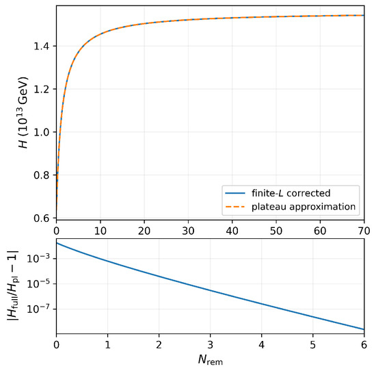
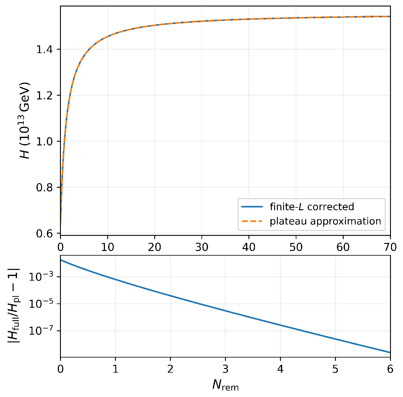
For the comparison plots below, $H_{\mathrm{full}}\left(N_{\mathrm{rem}}\right)$ denotes the finite-L result of Equation (110). Integrating $d\ln H/d{N}_{\mathrm{rem}}={ϵ}_1^{\mathrm{pl}}$ from the pivot $N_{\ast }$ to $N_{\mathrm{rem}}$ and normalizing to $H_{\ast }$ gives the asymptotic plateau history

$${\displaystyle \frac{H_{\mathrm{pl}}\left(N_{\mathrm{rem}}\right)}{H_{\ast }}}=\exp \left[-{\displaystyle \frac{{\alpha }_{\mathrm{eff}}}{N_{\mathrm{rem}}+\Delta }}+{\displaystyle \frac{{\alpha }_{\mathrm{eff}}}{N_{\ast }+\Delta }}\right].$$

(111)

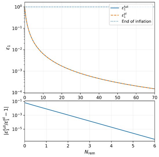
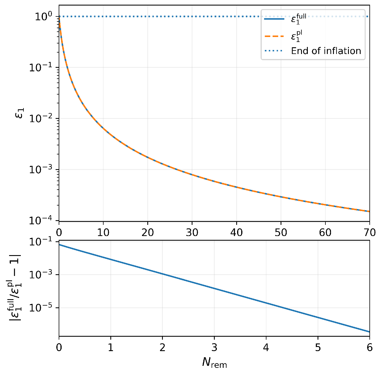
The finite-L and asymptotic plateau histories are compared in Figure 4 and Figure 5. The symbols $H_{\mathrm{full}}$ and $H_{\mathrm{pl}}$ in Figure 5 refer to these two normalized histories.

Figure 4. Finite-L corrected first Hubble-flow parameter and its asymptotic plateau approximation for the minimal benchmark. The upper panel shows the full $0\le N_{\mathrm{rem}}\le 70$ range; the curves are nearly indistinguishable over the CMB window. The lower panel resolves the endpoint region through the absolute fractional difference $|{ϵ}_1^{\mathrm{full}}/{ϵ}_1^{\mathrm{pl}}-1|$, showing explicitly where the plateau approximation ceases to be accurate. The Barnes-G matched full flow satisfies ${ϵ}_1^{\mathrm{full}}\left(0\right)=1$.

Figure 5. HBMB Hubble scale for the finite-L corrected benchmark and the asymptotic plateau approximation, with the absolute normalization fixed by $A_s=2.1\times {10}^{-9}$ at $N_{\ast }=55$ as described in Section 5. The upper panel shows the full inflationary window. The lower panel resolves $0\le N_{\mathrm{rem}}\le 6$ through the absolute fractional difference $|H_{\mathrm{full}}/H_{\mathrm{pl}}-1|$, making the finite-L endpoint correction visible without obscuring the near-degeneracy over the CMB window.

5. Scalar and Tensor Perturbations

Once the background flow is fixed, scalar and tensor perturbations obey the usual Mukhanov–Sasaki equations [46,47,48],

$$\begin{array}{cc}\hfill v_k^{″}+\left(k^2-{\displaystyle \frac{z^{″}}{z}}\right)v_k& =0,z=a\sqrt{2{ϵ}_1}{M}_P,\hfill \end{array}$$

(112)

$$\begin{array}{cc}\hfill u_k^{″}+\left(k^2-{\displaystyle \frac{a^{″}}{a}}\right)u_k& =0.\hfill \end{array}$$

(113)

Here, $v_k$ and $u_k$ are the scalar and tensor canonical mode functions, k is the comoving wave number, a is the scale factor, $z=a\sqrt{2{ϵ}_1}{M}_P$ is the standard scalar pump field, a itself plays the analogous role for tensors, $M_P$ is the reduced Planck mass, and primes denote derivatives with respect to conformal time. In the present treatment, we use the minimal canonical closure $c_s=1$, where $c_s$ is the scalar sound speed; HBMB physics enters through the projected background flow rather than through an additional sound-speed sector.

At leading slow-roll order [42,43,44], the scalar and tensor power spectra at the pivot scale $k_{\ast }$ are

$$\begin{array}{cc}\hfill {\mathcal{P}}_{\mathcal{R}}\left(k_{\ast }\right)& \simeq {\displaystyle \frac{H_{\ast }^2}{8{\pi }^2{M}_P^2{ϵ}_{1\ast }}}=A_s,\hfill \end{array}$$

(114)

$$\begin{array}{cc}\hfill {\mathcal{P}}_T\left(k_{\ast }\right)& \simeq {\displaystyle \frac{2H_{\ast }^2}{{\pi }^2{M}_P^2}}=r{A}_s,\hfill \end{array}$$

(115)

where ${\mathcal{P}}_{\mathcal{R}}$ denotes the curvature perturbation spectrum, ${\mathcal{P}}_T$ the tensor spectrum, and $A_s\equiv {\mathcal{P}}_{\mathcal{R}}\left(k_{\ast }\right)$ is the observed scalar-amplitude normalization. The pivot $k_{\ast }$ is the chosen comoving wavenumber whose horizon crossing occurs at $N_{\ast }=N_{\mathrm{rem}}\left(k_{\ast }\right)$. The corresponding spectral tilts are

$$n_s-1=-2{ϵ}_{1\ast }-{ϵ}_{2\ast },n_t\equiv {\displaystyle \frac{d\ln {\mathcal{P}}_T}{d\ln k}}{|}_{k_{\ast }}=-2{ϵ}_{1\ast },$$

(116)

with ${ϵ}_2$ defined in Equation (104). The scalar running is

$${\alpha }_s\equiv {\displaystyle \frac{d{n}_s}{d\ln k}}{|}_{k_{\ast }}\simeq -{\displaystyle \frac{d{n}_s}{d{N}_{\mathrm{rem}}}}{|}_{N_{\ast }}$$

(117)

at leading slow-roll order, where $d\ln k\simeq -d{N}_{\mathrm{rem}}$ at horizon crossing. For the minimal benchmark with $N_{\ast }=55$ and $A_s=2.1\times {10}^{-9}$, the leading-order relations give

$$\begin{array}{cc}\hfill H_{\ast }& =6.31562\times {10}^{-6}{M}_P\simeq 1.538\times {10}^{13}\mathrm{GeV},\hfill \end{array}$$

(118)

$$\begin{array}{cc}\hfill n_t& =-4.81119\times {10}^{-4},{\alpha }_s=-6.58725\times {10}^{-4}.\hfill \end{array}$$

(119)

Combining the scalar-amplitude normalization with the finite-flow ratio from Equation (110) gives

$$H_{\mathrm{end}}=H_{\mathrm{full}}\left(0\right)\simeq 2.65858\times {10}^{-6}{M}_P\simeq 6.474\times {10}^{12}\mathrm{GeV}.$$

(120)

Using the flat-FLRW Friedmann relation $\rho =3M_P^2{H}^2$ only as a characteristic total energy-density conversion gives

$${\rho }_{\ast }^{1/4}\simeq 8.05\times {10}^{15}\mathrm{GeV},{\rho }_{\mathrm{end}}^{1/4}\simeq 5.23\times {10}^{15}\mathrm{GeV}.$$

(121)

These quantities are total energy-density scales; in particular, ${\rho }_{\mathrm{end}}^{1/4}$ is not identified with a slow-roll potential value at the endpoint ${ϵ}_1=1$. These amplitude-dependent quantities do not alter the background matching. The benchmark therefore implies a red scalar tilt and a small tensor-to-scalar ratio.

The conceptual status of these numbers should be stated precisely. Within the reference-sector construction, the Schur projection controls the high-ℓ tail scaling and the single-species determinant fixes the residual running coefficient $b_{1\mathrm{sp}}$. The conversion of that running into the background flow additionally uses the explicit response and scale-mapping closures of Section 4. The values of $n_s$ and r quoted above are therefore observables of a benchmark member of the resulting conditional plateau class, not parameter-free predictions of the full HBMB microphysics.

6. Illustrative Tail-Decoupling Reheating Prescription and Dynamical Limitations

6.1. Status and Motivation

A standard perturbative decay width ${\mathsf{\Gamma }}_{\mathrm{dec}}$, as in conventional reheating treatments [27,28], can be attached to the projected HBMB background, but the projection formalism suggests an additional effective channel: as the accessible capacity grows and retained–omitted mixing weakens, the magnitude of the projected tail correction can decrease. The present section asks how such a decrease could be represented as an effective source for radiation. It is not a microscopic particle-production derivation, and it is not used to determine the determinant coefficients of Section 4.

To keep the time variables distinct from the backward inflationary coordinate $N_{\mathrm{rem}}$, we define the post-inflationary forward e-fold variable

$$\begin{array}{|c|}\hline \mathcal{N}\equiv \ln \left({\displaystyle \frac{a}{a_{\mathrm{end}}}}\right),{\displaystyle \frac{d\mathcal{N}}{dt}}=H.\\ \hline\end{array}$$

(122)

6.2. Adiabatic Tail-Decoupling Source

For an illustrative adiabatic prescription, let the positive tail-reservoir profile be proportional to the projected correction of Section 2,

$$\begin{array}{|c|}\hline {\rho }_{\mathrm{tail}}^{\mathrm{ad}}\left(\mathcal{N}\right)=C_{\mathrm{rh}}\Delta U_{\mathrm{HBMB}}\left(\mathcal{N}\right)\propto {\displaystyle \frac{1}{[N_{\mathrm{acc}}\left(\mathcal{N}\right)+\nu ][1+N_{\mathrm{acc}}\left(\mathcal{N}\right)/N_c]}}.\\ \hline\end{array}$$

(123)

Here, $N_{\mathrm{acc}}\left(\mathcal{N}\right)\equiv N_{\mathrm{acc}}\left[R\left(\mathcal{N}\right)\right]$ denotes the same screen-capacity variable introduced in Section 1, now evaluated along a post-inflationary screen trajectory; no microscopic form of $R\left(\mathcal{N}\right)$ is derived in this illustrative subsection. The constants $N_c$ and $\nu$ retain the meanings given in Section 2 and Section 3, and $C_{\mathrm{rh}}>0$ is an overall conversion factor. Equation (123) is a prescribed adiabatic profile used to estimate a possible release rate; it is not simultaneously assumed to be the solution of an independent continuity equation.

If this prescribed reservoir decreases, the positive energy released per unit cosmic time is

$$-{\displaystyle \frac{d{\rho }_{\mathrm{tail}}^{\mathrm{ad}}}{dt}}=-{\displaystyle \frac{d\mathcal{N}}{dt}}{\displaystyle \frac{d{\rho }_{\mathrm{tail}}^{\mathrm{ad}}}{d\mathcal{N}}}=-H{\displaystyle \frac{d{\rho }_{\mathrm{tail}}^{\mathrm{ad}}}{d\mathcal{N}}}.$$

(124)

If a fraction $0<\xi \le 1$ of that released energy is transferred to radiation, a minimal effective source prescription is therefore

$$\begin{array}{|c|}\hline Q_{\mathrm{rh}}^{\mathrm{ad}}\left(\mathcal{N}\right)=\xi H\max \left(0,-{\displaystyle \frac{d{\rho }_{\mathrm{tail}}^{\mathrm{ad}}}{d\mathcal{N}}}\right).\\ \hline\end{array}$$

(125)

The factor of H follows directly from Equation (122) and gives $Q_{\mathrm{rh}}^{\mathrm{ad}}$ the dimensions of energy density per unit time. The efficiency $\xi$ summarizes unresolved transfer microphysics; Equation  (125) should therefore be read as an adiabatic effective source functional rather than a microscopic decay law.

6.3. Possible Dynamical Completion

A self-consistent dynamical treatment must promote the tail reservoir to an independent variable rather than prescribing the same profile algebraically. Denoting that dynamical reservoir by ${\rho }_{\mathrm{tail}}$ and the radiation energy density by ${\rho }_r$, one possible two-component completion has the form

$$\begin{array}{cc}\hfill {\displaystyle \frac{d{\rho }_{\mathrm{tail}}}{d\mathcal{N}}}+3(1+w_{\mathrm{tail}}){\rho }_{\mathrm{tail}}& =-{\displaystyle \frac{Q_{\mathrm{rh}}}{H}},\hfill \end{array}$$

(126)

$$\begin{array}{cc}\hfill {\displaystyle \frac{d{\rho }_r}{d\mathcal{N}}}+4{\rho }_r& =+{\displaystyle \frac{Q_{\mathrm{rh}}}{H}},\hfill \end{array}$$

(127)

$$\begin{array}{cc}\hfill H^2& ={\displaystyle \frac{{\rho }_{\mathrm{tail}}+{\rho }_r}{3M_P^2}}.\hfill \end{array}$$

(128)

Here, $w_{\mathrm{tail}}$ is the effective equation-of-state parameter of the dynamical tail reservoir, and $Q_{\mathrm{rh}}$ is a generic energy-transfer rate (energy density per unit cosmic time). It need not equal the illustrative adiabatic source $Q_{\mathrm{rh}}^{\mathrm{ad}}$ of Equation (125); identifying the two would be an additional constitutive assumption. In such a completion, $Q_{\mathrm{rh}}$ and $w_{\mathrm{tail}}$ must be supplied by independent microscopic or constitutive information; Equation (123) should not at the same time be imposed as an exact dynamical trajectory. The adiabatic source of Equation (125) is therefore best regarded as an illustrative estimate of the transfer channel suggested by the decreasing projected tail.

6.4. Implications for the Observational e-Fold Number $N_{\ast }$

The pivot e-fold number is fixed only after a reheating and thermal history has been specified. Schematically, the mapping has the form

$$\begin{array}{|c|}\hline N_{\ast }=\mathcal{F}\left[{\alpha }_{\mathrm{eff}},\Delta ,Q_{\mathrm{rh}},w_{\mathrm{tail}},\mathrm{thermal}\mathrm{history}\right],\\ \hline\end{array}$$

(129)

where $\mathcal{F}$ denotes a model-dependent mapping functional summarizing the reheating and subsequent thermal history, with the HBMB tail entering through the chosen transfer prescription. Because neither $Q_{\mathrm{rh}}$ nor $w_{\mathrm{tail}}$ is microscopically closed here, the present work does not derive a unique $N_{\ast }$. The commonly used 50–60 e-fold interval is therefore retained only as a benchmark window for the observable calculations of Section 4 and Section 5.

7. Discussion

The logical status of the construction is most clearly separated into four layers. The first layer is the deparametrized operator framework. A concrete flat-FLRW plus free-scalar clock background leads to the positive operator ${\Theta }_{\mathrm{bg}}=-{\partial }_x^2$ and a well-defined positive-frequency evolution. The subsequent angular calculation is deliberately narrower: it is a normalized massless single-effective-species Laplace reference sector, not a derivation of the complete gauge-fixed Einstein–matter fluctuation operator. The HBMB capacity condition then defines the accessible/omitted $P/Q$ split in that reference sector.

The second layer is the retained–omitted coupling and its Schur tail. The explicit $S^2$ strip calculation gives the geometric overlap scaling $|V_{\mathit{\ell }}^{\mathrm{raw}}{|}^2\sim {\lambda }_{\mathit{\ell }}^{-1/2}$. For a one-dimensional retained coarse sector, rank one is kinematic and is not itself a physical prediction. The nontrivial geometric input is the raw strip-overlap envelope $|V_{\mathit{\ell }}^{\mathrm{raw}}|\sim {\mathit{\ell }}^{-1/2}$. The operator matrix element $V_{\mathit{\ell }}^{\mathrm{strip}}=\mathcal{G}\left(R\right)V_{\mathit{\ell }}^{\mathrm{raw}}$ inherits the same exponent. In the uniform channel basis ${\sigma }_{\mathit{\ell }}=\left|V_{\mathit{\ell }}^{\mathrm{strip}}\right|$, while bounded nonuniformity preserves ${\sigma }_{\mathit{\ell }}^2\sim {\mathit{\ell }}^{-1}$ under the stated condition; together with ${\lambda }_{\mathit{\ell }}\sim {\mathit{\ell }}^2$, this gives $K_{\mathit{\ell }}\sim {\mathit{\ell }}^{-3}$ and an $L^{-2}$ tail. The DFT channel basis, parity selection of a centered strip, and bounded-nonuniformity analysis clarify which parts of this scaling are geometric and which are representation dependent. The exactly telescoping kernel is therefore used as a convenient summable representative of the asymptotic class rather than as a uniquely derived microscopic interaction.

The third layer is the omitted-sector determinant. The exact integer sum and its large-L expansion show that the raw determinant contains bulk, interface, logarithmic, and inverse-power pieces. The $L^{-3}$ contribution is retained explicitly in the finite-L expansion. After the stated bulk and local cutoff-boundary subtraction, the normalized uncoupled one-species reference determinant obeys Equation (78) and fixes $b_{1\mathrm{sp}}=2/3$. This coefficient should not be interpreted as the already-computed coefficient of full quantum gravity: additional physical polarizations, matter sectors, gauge/ghost determinants, or diagonal Q-sector terms generated by a microscopic screen interaction can renormalize the full coefficient. Likewise, the Barnes-G construction used near the endpoint is the standard analytic continuation of the exact integer hyperfactorial expression; it supplies a controlled benchmark interpolation, not a new scheme-independent fundamental constant.

The fourth, cosmological, layer requires additional input. The determinant fixes $g_{1\mathrm{sp}}\left(L\right)$, while Equations (82) and (85) introduce, respectively, an effective background-response coefficient $c_{\chi }$ and an effective mapping coefficient $c_L$ between the HBMB capacity cutoff and remaining e-folds. Consequently,

$${\alpha }_{\mathrm{eff}}={\displaystyle \frac{c_{\chi }}{2b_{1\mathrm{sp}}{c}_L}}={\displaystyle \frac{3}{4}}{\displaystyle \frac{c_{\chi }}{c_L}}$$

for the one-species reference coefficient. The value $3/4$ is therefore the minimal $c_{\chi }=c_L=1$ benchmark, not a determinant-only prediction. Finite-L matching further depends separately on $c_L$. In that benchmark, the standard Barnes-G continuation gives ${\Delta }_{\mathrm{match}}^{\left(G\right)}\simeq 0.83665$, whereas ${\Delta }_{\mathrm{asy}}=\sqrt{3}/2$ belongs to the pure asymptotic plateau extrapolation. The distinction matters close to the end of inflation but changes the CMB-window benchmark only slightly.

The observable hierarchy is correspondingly asymmetric. At leading slow-roll order,

$$n_s=1-{\displaystyle \frac{2}{N_{\ast }+\Delta }}-{\displaystyle \frac{2{\alpha }_{\mathrm{eff}}}{{(N_{\ast }+\Delta )}^2}},r={\displaystyle \frac{16{\alpha }_{\mathrm{eff}}}{{(N_{\ast }+\Delta )}^2}}.$$

Thus, the dominant scalar-tilt term is weakly sensitive to the response normalization, while the tensor amplitude is directly proportional to ${\alpha }_{\mathrm{eff}}$. The minimal benchmark lies in the familiar Starobinsky/$\alpha$-attractor plateau region [30,31,32,33,34,35,36]. The present leading observables therefore do not provide a unique discriminant for HBMB; the proposed distinction is the spectral/capacity origin of the effective plateau running.

Finally, the reheating construction remains illustrative. The adiabatic source in Equation (125) gives a dimensionally and physically transparent way to parametrize release of a decreasing projected-tail reservoir, but it is not a microscopic particle-production law. A self-consistent dynamical completion requires an independently specified transfer law and reservoir equation of state. For the same reason, the observational pivot value $N_{\ast }$ is retained as a benchmark in the 50–60 range rather than being derived from the present reheating model.

The framework should therefore be read in four levels of control: the explicit deparametrized reference operator; controlled high-ℓ Schur-tail scaling; the renormalized single-species determinant running; and conditional cosmological consequences that depend on $c_{\chi }$, $c_L$, finite matching, and reheating assumptions. This narrower separation is also consistent with perturbative demonstrations that WDW constraints encode holographic information localization [16,17], while avoiding the stronger claim that the present paper has already constructed the complete gravitational fluctuation spectrum.

8. Conclusions

The main results of this paper, with their stated scope, are the following.

• A concrete flat-FLRW plus free homogeneous scalar clock gives the deparametrized background equation $[{\partial }_{\phi }^2+{\Theta }_{\mathrm{bg}}]\mathsf{\Psi }=0$ with ${\Theta }_{\mathrm{bg}}=-{\partial }_x^2$, making the positive-frequency branch explicit before the HBMB projection is introduced. The subsequent angular determinant is a normalized single-effective-species reference sector rather than the complete Einstein–matter fluctuation operator.
• The holographic capacity and angular channel count are separated through $I_{\mathrm{acc}}^{\mathrm{tot}}=\ln \dim {\mathcal{H}}_{\mathrm{acc}}$ and the capacity-charged quantity $I_{\mathrm{acc}}^{\mathrm{cap}}=I_{\mathrm{acc}}^{\mathrm{tot}}-I_{\mathrm{seed}}$. In the reference angular sector, the capacity cutoff defines the accessible/omitted $P/Q$ split without identifying thermodynamic entropy directly with a number of harmonics.
• The explicit $S^2$ strip model gives the nontrivial geometric input $|V_{\mathit{\ell }}^{\mathrm{raw}}{|}^2\sim {\lambda }_{\mathit{\ell }}^{-1/2}$. The normalized operator matrix element $V_{\mathit{\ell }}^{\mathrm{strip}}=\mathcal{G}\left(R\right)V_{\mathit{\ell }}^{\mathrm{raw}}$ inherits the same exponent. In the uniform channel basis, ${\sigma }_{\mathit{\ell }}=\left|V_{\mathit{\ell }}^{\mathrm{strip}}\right|$; together with ${\lambda }_{\mathit{\ell }}\sim {\mathit{\ell }}^2$, this produces $K_{\mathit{\ell }}\sim {\mathit{\ell }}^{-3}$ and an $L^{-2}$ omitted-tail class. Centered-strip parity and bounded nonuniform channel weights do not change this asymptotic exponent under the stated conditions.
• The exactly summable representative kernel yields $\Delta U_{\mathrm{HBMB}}\propto {(N_{\mathrm{acc}}+\nu )}^{-1}$. The Section 3 effective-fluid and capacity-suppressed exit constructions are illustrative closures built on that tail scaling, not microscopic energy-transfer derivations.
• For the normalized uncoupled single-species Q sector, the renormalized determinant is

  $${\mathsf{\Gamma }}_Q^{\mathrm{ren}}\left(L\right)={\mathsf{\Gamma }}_0-{\displaystyle \frac{2}{3}}\ln L-{\displaystyle \frac{31}{360L^2}}+{\displaystyle \frac{1}{12L^3}}+O\left(L^{-4}\right),$$

  so that the reference logarithmic coefficient is $b_{1\mathrm{sp}}=2/3$. The explicit $L^{-3}$ term is important for controlling the approach to the finite-L matching regime.
• After introducing the explicit effective response and cutoff–e-fold mapping coefficients, the leading conditional plateau class is

  $${ϵ}_1\simeq {\displaystyle \frac{{\alpha }_{\mathrm{eff}}}{{(N_{\mathrm{rem}}+\Delta )}^2}},{\alpha }_{\mathrm{eff}}={\displaystyle \frac{3}{4}}{\displaystyle \frac{c_{\chi }}{c_L}}.$$
  For the minimal benchmark $c_{\chi }=c_L=1$, standard Barnes-G continuation gives ${\Delta }_{\mathrm{match}}^{\left(G\right)}\simeq 0.83665$ and, at $N_{\ast }=55$,

  $$n_s\simeq 0.963700,r\simeq 3.849\times {10}^{-3}.$$
  These are benchmark values of the conditional reference realization, not parameter-free predictions of complete HBMB microphysics. In particular, $n_s$ is weakly closure-sensitive at leading order, whereas r depends directly on the response normalization.
• The reheating source is retained as an illustrative adiabatic prescription. A microscopic transfer law and a self-consistent thermal history are still required before $N_{\ast }$ can be predicted rather than treated as a benchmark window.

The next steps are correspondingly well defined. A full microscopic implementation would need the gauge-fixed Einstein–matter fluctuation operator, including physical polarizations, gauge/ghost sectors, and any diagonal Q-sector contributions associated with the screen interaction. It would also need independent derivations of the response coefficient $c_{\chi }$ and of the physical screen evolution that determines $c_L$, followed by a microscopic reheating mechanism. These extensions are outside the present work. The result established here is narrower: a finite HBMB capacity regularization with an explicit deparametrized projection, controlled high-ℓ tail scaling, a reproducible single-species determinant running, and clearly separated conditional cosmological consequences.

References

- Arnowitt, R.; Deser, S.; Misner, C.W. The Dynamics of General Relativity. In Gravitation: An Introduction to Current Research; Witten, L., Ed.; Wiley: New York, NY, USA, 1962. [Google Scholar]
- DeWitt, B.S. Quantum Theory of Gravity. I. The Canonical Theory. Phys. Rev. 1967, 160, 1113. [Google Scholar] [CrossRef] [Scilit]
- Halliwell, J.J. Introductory lectures on quantum cosmology. In Quantum Cosmology and Baby Universes; Coleman, S., Hartle, J.B., Piran, T., Weinberg, S., Eds.; World Scientific: Singapore, 1991. [Google Scholar]
- Kiefer, C. Quantum Gravity, 3rd ed.; Oxford University Press: Oxford, UK, 2012. [Google Scholar]
- Isham, C.J. Canonical quantum gravity and the problem of time. In Integrable Systems, Quantum Groups, and Quantum Field Theories; NATO ASI Series C; Kluwer: Alphen aan den Rijn, The Netherlands, 1993; Volume 409. [Google Scholar]
- Kuchař, K.V. Time and interpretations of quantum gravity. In Proceedings of the 4th Canadian Conference on General Relativity and Relativistic Astrophysics; Kunstatter, G., Vincent, D., Williams, J., Eds.; World Scientific: Singapore, 1992. [Google Scholar]
- Hartle, J.B.; Hawking, S.W. Wave function of the Universe. Phys. Rev. D 1983, 28, 2960. [Google Scholar] [CrossRef] [Scilit]
- Vilenkin, A. Boundary conditions in quantum cosmology. Phys. Rev. D 1986, 33, 3560. [Google Scholar] [CrossRef] [Scilit] [PubMed]
- Bekenstein, J.D. Black holes and entropy. Phys. Rev. D 1973, 7, 2333. [Google Scholar] [CrossRef] [Scilit]
- Hawking, S.W. Particle creation by black holes. Commun. Math. Phys. 1975, 43, 199. [Google Scholar] [CrossRef] [Scilit]
- ’t Hooft, G. Dimensional reduction in quantum gravity. arXiv 1993, arXiv:gr-qc/9310026. [Google Scholar]
- Susskind, L. The World as a hologram. J. Math. Phys. 1995, 36, 6377. [Google Scholar] [CrossRef] [Scilit]
- Jacobson, T. Thermodynamics of spacetime: The Einstein equation of state. Phys. Rev. Lett. 1995, 75, 1260. [Google Scholar] [CrossRef] [Scilit] [PubMed]
- Hartnoll, S.A. Wheeler-DeWitt states of the AdS-Schwarzschild interior. J. High Energy Phys. 2023, 2023, 66. [Google Scholar] [CrossRef] [Scilit]
- Araujo-Regado, G.; Khan, R.; Wall, A.C. Cauchy slice holography: A new AdS/CFT dictionary. J. High Energy Phys. 2023, 2023, 26. [Google Scholar] [CrossRef] [Scilit]
- Chowdhury, C.; Godet, V.; Papadoulaki, O.; Raju, S. Holography from the Wheeler-DeWitt equation. J. High Energy Phys. 2022, 2022, 19. [Google Scholar] [CrossRef] [Scilit]
- Chakraborty, T.; Chakravarty, J.; Godet, V.; Paul, P.; Raju, S. Holography of information in de Sitter space. J. High Energy Phys. 2023, 2023, 120. [Google Scholar] [CrossRef] [Scilit]
- Nagy, D. Basics of a Geometry-Independent HBMB Holographic Principle: From Horizon Bits to Bulk Wavefunctions—Part I. Preprints 2026, 2026011465. [Google Scholar]
- Nagy, D. U(1)-Driven Local Holographic Screens (Horizons): Holographic Bit–Mode Balance and the α-Fixpoint. Preprints 2025, 2025111803. [Google Scholar]
- Nagy, D. A First-Principles Derivation of the Fine-Structure Constant from Holographic Bit–Mode Balance. OSF Preprints. 2025. Available online: https://osf.io/hw2je (accessed on 26 August 2026).
- Nagy, D. Holographic Vacuum Energy from Quantized Horizons. OSF Preprints. 2025. Available online: https://osf.io/m8t6h (accessed on 26 August 2026).
- Feshbach, H. Unified theory of nuclear reactions. Ann. Phys. 1958, 5, 357. [Google Scholar] [CrossRef] [Scilit]
- Feshbach, H. A unified theory of nuclear reactions. II. Ann. Phys. 1962, 19, 287. [Google Scholar] [CrossRef] [Scilit]
- Ashtekar, A.; Pawłowski, T.; Singh, P. Quantum nature of the big bang. Phys. Rev. Lett. 2006, 96, 141301. [Google Scholar] [CrossRef] [Scilit] [PubMed]
- Ashtekar, A.; Pawłowski, T.; Singh, P. Quantum nature of the big bang: An analytical and numerical investigation. Phys. Rev. D 2006, 73, 124038. [Google Scholar] [CrossRef] [Scilit]
- Ashtekar, A.; Singh, P. Loop quantum cosmology: A status report. Class. Quantum Grav. 2011, 28, 213001. [Google Scholar] [CrossRef] [Scilit]
- Kofman, L.; Linde, A.; Starobinsky, A.A. Towards the theory of reheating after inflation. Phys. Rev. D 1997, 56, 3258. [Google Scholar] [CrossRef] [Scilit]
- Allahverdi, R.; Brandenberger, R.; Cyr-Racine, F.-Y.; Mazumdar, A. Reheating in inflationary cosmology: Theory and applications. Ann. Rev. Nucl. Part. Sci. 2010, 60, 27. [Google Scholar] [CrossRef] [Scilit]
- Cook, J.L.; Dimastrogiovanni, E.; Easson, D.A.; Krauss, L.M. Reheating predictions in single field inflation. J. Cosmol. Astropart. Phys. 2015, 2015, 47. [Google Scholar] [CrossRef] [Scilit]
- Starobinsky, A.A. A new type of isotropic cosmological models without singularity. Phys. Lett. B 1980, 91, 99. [Google Scholar] [CrossRef] [Scilit]
- Kallosh, R.; Linde, A. Universality class in conformal inflation. J. Cosmol. Astropart. Phys. 2013, 2013, 2. [Google Scholar] [CrossRef] [Scilit]
- Kallosh, R.; Linde, A.; Roest, D. Superconformal inflationary α-attractors. J. High Energy Phys. 2013, 2013, 198. [Google Scholar] [CrossRef] [Scilit]
- Roest, D. Universality classes of inflation. J. Cosmol. Astropart. Phys. 2014, 2014, 7. [Google Scholar] [CrossRef] [Scilit]
- Martin, J.; Ringeval, C.; Vennin, V. Encyclopaedia Inflationaris. Phys. Dark Univ. 2014, 5, 75–235. [Google Scholar] [CrossRef] [Scilit]
- Akrami, Y.; Planck Collaboration. Planck 2018 results. X. Constraints on inflation. Astron. Astrophys. 2020, 641, A10. [Google Scholar]
- Ade, P.A.R.; BICEP/Keck Collaboration. Improved constraints on primordial gravitational waves using BICEP/Keck 2018 data. Phys. Rev. Lett. 2021, 127, 151301. [Google Scholar] [CrossRef] [Scilit] [PubMed]
- Olver, F.W.J.; Olde Daalhuis, A.B.; Lozier, D.W.; Schneider, B.I.; Boisvert, R.F.; Clark, C.W.; Miller, B.R.; Saunders, B.V.; Cohl, H.S.; McClain, M.A. (Eds.) NIST Digital Library of Mathematical Functions; National Institute of Standards and Technology: Gaithersburg, MD, USA, 2003. Available online: https://dlmf.nist.gov/ (accessed on 19 August 2026).
- Birrell, N.D.; Davies, P.C.W. Quantum Fields in Curved Space; Cambridge University Press: Cambridge, UK, 1982. [Google Scholar]
- Vassilevich, D.V. Heat kernel expansion: User’s manual. Phys. Rep. 2003, 388, 279. [Google Scholar] [CrossRef] [Scilit]
- Dunne, G.V. Functional determinants in quantum field theory. J. Phys. A 2008, 41, 304006. [Google Scholar] [CrossRef] [Scilit]
- Kirsten, K. Spectral Functions in Mathematics and Physics; CRC Press: Boca Raton, FL, USA, 2001. [Google Scholar]
- Mukhanov, V. Physical Foundations of Cosmology; Cambridge University Press: Cambridge, UK, 2005. [Google Scholar]
- Liddle, A.R.; Lyth, D.H. Cosmological Inflation and Large-Scale Structure; Cambridge University Press: Cambridge, UK, 2000. [Google Scholar]
- Baumann, D. TASI Lectures on Inflation. arXiv 2009, arXiv:0907.5424. [Google Scholar]
- Sidan, A.; Banks, T. Holographic spacetime model of inflation and its predictions for the CMB primordial spectra. Phys. Rev. D 2025, 112, 023516. [Google Scholar]
- Mukhanov, V.F.; Chibisov, G.V. Quantum fluctuations and a nonsingular universe. J. Exp. Theor. Phys. Lett. 1981, 33, 532–535. [Google Scholar]
- Sasaki, M. Large scale quantum fluctuations in the inflationary universe. Prog. Theor. Phys. 1986, 76, 1036. [Google Scholar] [CrossRef] [Scilit]
- Mukhanov, V.F. Quantum theory of gauge-invariant cosmological perturbations. Sov. Phys. J. Exp. Theor. Phys. 1988, 67, 1297–1302. [Google Scholar]
Disclaimer/Publisher’s Note: The statements, opinions and data contained in all publications are solely those of the individual author(s) and contributor(s) and not of MDPI and/or the editor(s). MDPI and/or the editor(s) disclaim responsibility for any injury to people or property resulting from any ideas, methods, instructions or products referred to in the content. |
© 2026 by the author. Licensee MDPI, Basel, Switzerland. This article is an open access article distributed under the terms and conditions of the Creative Commons Attribution (CC BY) license.