Influence of Fast and Slow Laser Phase Noise on the Fidelity of the Mølmer–Sørensen Trapped-Ion Gate

Abstract

High-fidelity two-qubit entangling gates are essential for the realization of useful quantum algorithms on quantum processors. The Mølmer–Sørensen (MS) gate has become a common choice for trapped-ion quantum computing due to its resilience to ion temperature and its demonstrated record fidelities. However, the spectral impurity of the driving laser field impacts gate performance, with phase noise influencing the qubit dynamics through mechanisms operating on different timescales. In this work, we present a comprehensive theoretical analysis of laser phase noise in the MS gate, identifying two spectral ranges that influence the gate fidelity the most: “fast” noise at frequencies near the motional mode spectrum, and “slow” noise at frequencies on the order of the inverse gate time. We derive the noise Hamiltonians for two common laser beam geometries and obtain analytical expressions for the average gate error in terms of the laser noise power spectral density and gate parameters. For slowly varying noise spectra, we provide simplified error estimates. In addition, we validate our findings against previously published numerical simulations.

1. Introduction

The anticipated progress in the development of large- and intermediate-scale quantum computers [1,2,3] relies on the ability to perform high-fidelity gates in many-qubit quantum registers. Although there are algorithmic methods of compensating for imperfect gates, such as error correction [4] and error mitigation [5], the computational and/or experimental overhead imposed by these methods may significantly reduce their advantage and limit their applicability. Thus, it remains an important task to identify, study and suppress the various physical mechanisms that lead to gate errors.

Among all physical platforms for quantum computation, trapped ions continue to prove their efficacy, having already demonstrated record one- and two-qubit gate fidelities [6] and quantum volume [7], with recent larger-scale high-connectivity systems approaching 100 qubits [3]. The long-range strong Coulomb interaction between the ions, as well as the invention of the quantum charge-coupled device (QCCD) architecture [8], allow efficient and flexible scaling and high-fidelity entanglement [9,10].

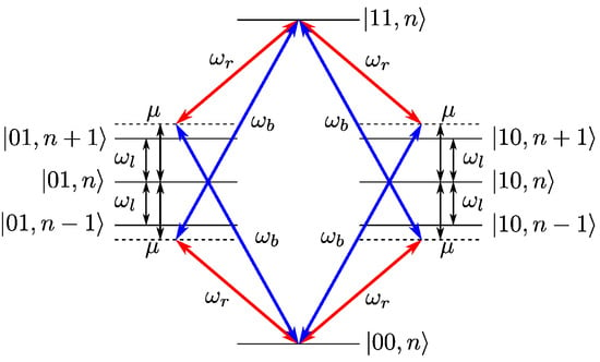
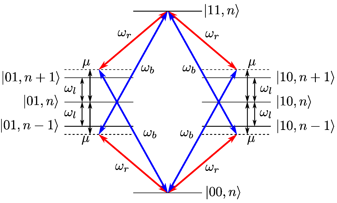
One of the major challenges, characteristic of any platform, is the fidelity of two-qubit entangling gates. Any universal quantum computer requires at least one such gate to be able to perform any unitary transformation of the whole register with a given accuracy in finite time [4]. With trapped ions in particular, one common choice is the Mølmer–Sørensen (MS) gate [11,12]. In the original proposal, it invokes a bichromatic laser field, which contains two frequency components, symmetrically detuned (by $\pm \mu$) from the qubit carrier transition, called the red and blue components (Figure 1). The detuning is chosen close to one of the motional modes of the ionic chain in the trap, creating four Raman-like stimulated transitions, with the intermediate states being the motional sidebands. Due to interference between the transitions, the effective frequency of the Rabi cycle between states $\left|00\right.⟩ \mathrm{and} \left|11\right.⟩$ will be independent on the motional number n. This is the main reason the MS gate is used extensively in many setups that show high two-qubit fidelities [6,13,14]. Although the original idea assumed that the transition $\left|0\right.⟩\to \left|1\right.⟩$ is an optical transition capable of being excited directly by each laser beam, the description is valid for hyperfine qubits driven by two Raman laser beams [15,16], or even for laser-free setups [6,17,18].

Figure 1. The MS gate level scheme. The bichromatic field (${\omega }_b,{\omega }_r$) creates 4 Raman paths between states $\left|00,n\right.⟩\leftrightarrow \left|11,n\right.⟩$. The intermediate states are the blue and red motional sidebands of the l-th mode with frequency ${\omega }_l$.

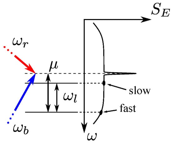
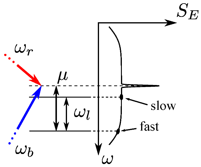
By construction of the MS gate, it is clear that its fidelity will be sensitive to phase fluctuations of the fields driving it, since the Raman process described above requires coherence between the two bichromatic components. All those components for all ions are usually generated by a single laser source, which then has its radiation split into several beams and then modulated with various optoelectronics. Therefore, the intrinsic phase noise of this source will transfer onto every field present in the gate. This will lead to the bichromatic components depicted in Figure 1 having acquired an identical spectrum $S_E\left(\omega \right)$ in terms of the electric field power spectral density (PSD), which is centered at the intermediate point between the red and blue parts (see Figure 2) and is related to the phase noise PSD [19]. This spectrum will, in general, overlap with the levels of the quantum system closest to the central peak, causing non-resonant parasitic transitions to and from these levels. This is similar to how a small perturbation with a continuous spectrum causes transitions between discrete levels with a rate obtained by applying the Fermi’s golden rule.

Figure 2. The influence of laser phase noise on the MS gate. Parasitic interactions arise from the overlap of the laser field power spectral density (PSD) $S_E\left(\omega \right)$ with the closest states of the system, outlining the “slow” and “fast” parts (see main text).

There are two most significant interactions that influence the MS gate error. The first one is the interaction with the carrier transition $\left|0,n\right.⟩\to \left|1,n\right.⟩$. It is caused by the Fourier components of the phase noise that have frequencies close to the detuning $\mu$. Since this detuning is, in turn, close to the motional frequencies of the ions (hundreds of kHz to several MHz), the timescales at which this noise is present are on the order of the oscillation period in the trap ($\sim$1 μs and less). At these high frequencies the main physical source of phase noise is the servo loop which is used to lock the laser to a stable reference, such as a high-finesse Fabry–Pérot cavity [20,21,22,23]. At frequencies around the servo bandwidth (which also lies in the MHz range [24,25]), the noise of the free-running laser is amplified instead of being suppressed, causing the so-called servo bumps [24]. These bumps have, therefore, a sizable effect on the fidelity of the MS gate, if they have a sufficient spectral overlap with the carrier transition. Another source of high-frequency errors are the relaxation oscillations of the gain medium. For solid state lasers, the relaxation oscillation peak in the phase noise spectrum lies in the sub-MHz range [25,26,27,28] and is thus also able to contribute to the gate error. Due to the small timescale of the described interaction, we call this noise the “fast” noise, since usually the gate time is much larger than the trap oscillation period.

The second interaction is the interaction with the first motional sidebands $\left|0,n\right.⟩\to \left|1,n\pm 1\right.⟩$ The relevant noise components in this case are on the order of $\mu -{\omega }_l$ and lie in the kHz to tens of kHz range. This frequency is approximately the inverse gate time, so the timescale for this type of noise is $0.1÷1$ ms. Moreover, frequency deviations of the laser that are slower than this timescale but have a large magnitude ($\lesssim \mu -{\omega }_l$) can lead to significant errors due to the bichromatic components being close to the resonance with the sideband transition. This “slow” noise (compared to the “fast” noise described above) can be caused by acoustic or thermal effects, and in the case of a cavity-stabilized laser, they are mainly tied to the mechanical properties of the cavity itself, owing to the large servo gain at such frequencies. These sources yield a $1/f$ frequency noise PSD [29,30]. Another source with the same $1/f$ PSD is the flicker noise, which is present in almost any electronic device, including the servo loop which locks the laser to the cavity. Technical and flicker noise together provide the low-frequency part of laser noise with a cutoff frequency of $10÷100\mathrm{Hz}$ [31,32], above which it is overtaken by white noise with a flat PSD [25,31,32].

To our knowledge, there seems to be limited attention to the two described types of noise in the literature. Despite the existence of various methods of reducing the influence of phase noise, such as using decoherence-free subspaces [33,34,35,36,37], as well as dynamical decoupling techniques [38,39,40,41], they only deal with pure dephasing, whereas the noise described above causes parasitic interactions, which these methods fail to adequately address. Fast laser noise of this type was studied in [24]; however, the authors estimated the error induced by this noise from numerical simulations, without calculating the error analytically. Time-varying noise of the laser phase was analyzed in [42], but the analysis there was confined to a specific laser beam geometry, and only fluctuations in the beam optical paths were considered, not the inherent phase noise of the common laser source which produces all individual addressing fields.

Here, we perform a theoretical analysis of intrinsic phase noise of the laser in the MS gate. We derive the noise terms in the Hamiltonian for both spectral ranges (fast and slow) and for all common beam geometries. We show that the average gate error is equal to the convolution between the phase or frequency noise PSD (depending on whether fast or slow noise is considered, respectively) and the so-called filter function of the gate, with the latter only depending on the gate parameters. We obtain analytical expressions for the filter functions, as well as giving simplified estimates for the error in trivial cases. Note that, despite our theory assuming laser radiation, as in the original description of the MS gate, it is applicable to all alternative gate setups mentioned earlier. Our findings complement previously published literature in two main ways. The first original result are the analytical expressions for the filter functions in both common beam geometries and both fast and slow spectral ranges. These filter functions expand on the filter function theory for trapped ions developed in [42], where a different noise source was studied. The second original result are the simplified estimations of the average error, which not only confirm the numerical simulations from [24], but also can be used as a rule of thumb for calculating the requirements on the spectral purity of the laser given the needed gate error.

In Section 2.1, we derive the MS gate Hamiltonians for two commonly used laser beam configurations (see below) and define the noise terms contributing to fast and slow noise. Section 2.2 and Section 2.3 are devoted to calculating the filter functions for the fast and slow parts of the noise, respectively. Section 3 presents the visual graphs of the calculated filter functions, as well as estimates of the total gate error in the simplest cases. We discuss our results and compare them to the findings of previously published works in Section 4.

2. Materials and Methods

2.1. Phase-Sensitive and Phase-Insensitive MS Gate Hamiltonians

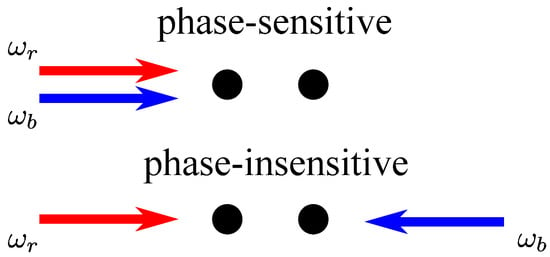
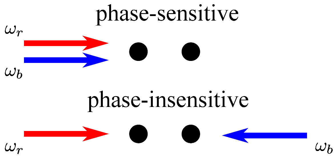
We start by deriving the MS gate Hamiltonians for the two most widely used laser field configurations: phase-sensitive and phase-insensitive [43]. In the phase-sensitive geometry, the bichromatic beam components are co-propagating, whereas in the phase-insensitive geometry they are counter-propagating (Figure 3).

Figure 3. The phase-sensitive and phase-insensitive laser beam geometries. In this example the axial motional modes of the ionic chain are excited.

The names of the configurations come from the different sensitivity of the entangling term in the evolution operator to fluctuations in the beams’ optical paths [43]. In both cases, we assume the intensities of the bichromatic components to be equal at the ion’s position. The Hamiltonian for both configurations will have the following form:

$$\begin{array}{c}{\widehat{H}}_{\mathrm{MS}}\left(t\right)=\sum _j{\displaystyle \frac{{\mathsf{\Omega }}_j}{2}}\left\{\left[{\sigma }_{+}^{\left(j\right)}\exp \left(\pm i\sum _l{\eta }_{lj}({\widehat{a}}_l{e}^{-i{\omega }_{l}t}+{\widehat{a}}_l^{†}{e}^{i{\omega }_{l}t})\right)e^{i({\varphi }_b^{(j)}-\mu t)}+\mathrm{h}.\mathrm{c}.\right]\right.\hfill \\ \hfill \hspace{1em}\hspace{1em}\hspace{1em}\hspace{1em}\hspace{1em}\hspace{1em}\hspace{1em}\hspace{1em} \left.+\left[{\sigma }_{+}^{\left(j\right)}\exp \left(\pm i\sum _l{\eta }_{lj}({\widehat{a}}_l{e}^{-i{\omega }_{l}t}+{\widehat{a}}_l^{†}{e}^{i{\omega }_{l}t})\right)e^{i({\varphi }_r^{(j)}+\mu t)}+\mathrm{h}.\mathrm{c}.\right]\right\},\end{array}$$

(1)

where ${\mathsf{\Omega }}_j$ is the Rabi frequency of the bichromatic field (the index j denotes the $j\mathrm{th}$ ion), ${\sigma }_{+}^{\left(j\right)}$ is the raising Pauli matrix, and ${\eta }_{lj}$ the Lamb–Dicke parameter of the $l\mathrm{th}$ motional mode with frequency ${\omega }_l$ and ladder operators ${\widehat{a}}_l,{\widehat{a}}_l^{†}$. The phases of the red and blue field components are ${\varphi }_r^{\left(j\right)}$ and ${\varphi }_b^{\left(j\right)}$ respectively, and their detuning relative to the carrier transition is symmetric and equal to $\mu$. Note that this expression is valid for both purely optical transitions and hyperfine Raman transitions, as long as the Lamb–Dicke parameters are defined properly [44]. The signs ± are picked according to the specific laser field configuration; see below.

2.1.1. Phase-Sensitive Configuration

In this configuration, both signs are chosen as “+”. In the Lamb–Dicke regime, the full Hamiltonian can be reduced to

$${\widehat{H}}_{\mathrm{MS}}^{\left(\mathrm{S}\right)}\left(t\right)\approx \sum _j{\mathsf{\Omega }}_j{\sigma }_{{\varphi }_{\perp }}^{\left(j\right)}\cos (\mu t+{\varphi }_M^{(j)})-\sum _{l,j}{\eta }_{lj}{\mathsf{\Omega }}_j{\sigma }_{\varphi }^{\left(j\right)}\cos (\mu t+{\varphi }_M^{\left(j\right)})({\widehat{a}}_l{e}^{-i{\omega }_{l}t}+{\widehat{a}}_l^{†}{e}^{i{\omega }_{l}t}),$$

(2)

where the “rotated” Pauli matrices are

$$\begin{array}{cc}\hfill {\sigma }_{{\varphi }_{\perp }}^{\left(j\right)}& ={\sigma }_x^{\left(j\right)}\cos {\varphi }_S^{\left(j\right)}-{\sigma }_y^{\left(j\right)}\cos {\varphi }_S^{\left(j\right)},\hfill \\ \hfill {\sigma }_{\varphi }^{\left(j\right)}& ={\sigma }_x^{\left(j\right)}\cos {\varphi }_S^{\left(j\right)}+{\sigma }_y^{\left(j\right)}\cos {\varphi }_S^{\left(j\right)},\hfill \end{array}$$

(3)

and the motional and spin phases ${\varphi }_M^{\left(j\right)},{\varphi }_S^{\left(j\right)}$ are defined as

$${\varphi }_{S,M}^{\left(j\right)}=({\varphi }_r^{\left(j\right)}\pm {\varphi }_b^{\left(j\right)})/2.$$

(4)

2.1.2. Phase-Insensitive Configuration Hamiltonian

In this configuration, one sign is “+”, while the other is “−”. Keeping the same definitions from above, the Hamiltonian in the Lamb–Dicke regime is

$${\widehat{H}}_{\mathrm{MS}}^{\left(\mathrm{I}\right)}\left(t\right)\approx \sum _j{\mathsf{\Omega }}_j{\sigma }_{{\varphi }_{\perp }}^{\left(j\right)}\cos (\mu t+{\varphi }_M^{\left(j\right)})+\sum _{l,j}{\eta }_{lj}{\mathsf{\Omega }}_j{\sigma }_{{\varphi }_{\perp }}^{\left(j\right)}\sin (\mu t+{\varphi }_M^{\left(j\right)})({\widehat{a}}_l{e}^{-i{\omega }_{l}t}+{\widehat{a}}_l^{†}{e}^{i{\omega }_{l}t}).$$

(5)

2.1.3. Laser Noise Terms

The noise terms in the above Hamiltonians come from fluctuations of the phases ${\varphi }_r^{\left(j\right)}$ and ${\varphi }_b^{\left(j\right)}$. If both bichromatic components come from the same source, which is usually the case [6,15,45,46], their fluctuations are identical to the fluctuations in the source. This means that, according to (4), only the phase ${\varphi }_S^{\left(j\right)}$ is affected:

$$\delta {\varphi }_S^{\left(j\right)}\left(t\right)=\delta \varphi \left(t\right),\delta {\varphi }_M^{\left(j\right)}\left(t\right)=0,$$

(6)

where $\delta \varphi \left(t\right)$ is the phase noise of the laser source. These fluctuations, in turn, lead to the following fluctuations in the spin operators:

$$\begin{array}{c}\hfill {\sigma }_{\varphi }^{\left(j\right)}\left(t\right)\approx {\sigma }_{\varphi }^{\left(j\right)}+{\sigma }_{{\varphi }_{\perp }}^{\left(j\right)}\delta \varphi \left(t\right),\\ \hfill {\sigma }_{{\varphi }_{\perp }}^{\left(j\right)}\left(t\right)\approx {\sigma }_{{\varphi }_{\perp }}^{\left(j\right)}-{\sigma }_{\varphi }^{\left(j\right)}\delta \varphi \left(t\right).\end{array}$$

(7)

Inserting these expressions into (2) and (5), we obtain the noise terms for the phase-sensitive configuration:

$$\begin{array}{c}{\widehat{V}}^{\left(\mathrm{S}\right)}\left(t\right)=-\delta \varphi \left(t\right)\left[\sum _j{\mathsf{\Omega }}_j{\sigma }_{\varphi }^{\left(j\right)}\cos (\mu t+{\varphi }_M^{\left(j\right)})\right.\hfill \\ \hfill \left.\hspace{1em}\hspace{1em}\hspace{1em}\hspace{1em}\hspace{1em}\hspace{1em}\hspace{1em}\hspace{1em}\hspace{1em}\hspace{1em}\hspace{1em}\hspace{1em}\hspace{1em} +\sum _{l,j}{\eta }_{lj}{\mathsf{\Omega }}_j{\sigma }_{{\varphi }_{\perp }}^{\left(j\right)}\cos (\mu t+{\varphi }_M^{\left(j\right)})({\widehat{a}}_l{e}^{-i{\omega }_{l}t}+{\widehat{a}}_l^{†}{e}^{i{\omega }_{l}t})\right],\end{array}$$

(8)

and for the phase-insensitive configuration:

$$\begin{array}{c}{\widehat{V}}^{\left(\mathrm{I}\right)}\left(t\right)=-\delta \varphi \left(t\right)\left[\sum _j{\mathsf{\Omega }}_j{\sigma }_{\varphi }^{\left(j\right)}\cos (\mu t+{\varphi }_M^{\left(j\right)})\right.\hfill \\ \hfill \left.\hspace{1em}\hspace{1em}\hspace{1em}\hspace{1em}\hspace{1em}\hspace{1em}\hspace{1em}\hspace{1em}\hspace{1em}\hspace{1em}\hspace{1em}\hspace{1em}\hspace{1em} +\sum _{l,j}{\eta }_{lj}{\mathsf{\Omega }}_j{\sigma }_{\varphi }^{\left(j\right)}\sin (\mu t+{\varphi }_M^{\left(j\right)})({\widehat{a}}_l{e}^{-i{\omega }_{l}t}+{\widehat{a}}_l^{†}{e}^{i{\omega }_{l}t})\right].\end{array}$$

(9)

The two sums in square brackets for each configuration represent the fast and slow parts of the noise, respectively, due to the reasons provided in the introduction. Furthermore, the separation between the relevant spectral ranges of the noise terms allows their independent treatment, since their spectral overlap is insignificant.

2.1.4. Mean Noisy Gate Fidelity

In a general qubit system, the Hamiltonian of a noisy gate can be written as

$$\widehat{H}\left(t\right)={\widehat{H}}_0\left(t\right)+\widehat{V}\left(t\right),$$

(10)

where ${\widehat{H}}_0\left(t\right)$ is the ideal Hamiltonian and $\widehat{V}\left(t\right)$ is the noise. The full evolution operator can be represented in the following way:

$$\widehat{U}={\widehat{U}}_0(1-i\widehat{T}),$$

(11)

where ${\widehat{U}}_0$ is the evolution operator with only ${\widehat{H}}_0$ (ideal evolution) and $\widehat{T}$ is the noise correction. We define the fidelity of a noisy gate with a specific starting state $\left|{\psi }_0\right.⟩$ as

$$F={\left|\left.⟨{\psi }_0\right|{\widehat{U}}_0^{†}\widehat{U}\left|{\psi }_0\right.⟩\right|}^2.$$

(12)

The gate error is then [47]

$$ϵ\left({\psi }_0\right)=1-F=\left.⟨{\psi }_0\right|{\widehat{T}}^{†}\widehat{T}\left|{\psi }_0\right.⟩-{\left|\left.⟨{\psi }_0\right|\widehat{T}\left|{\psi }_0\right.⟩\right|}^2.$$

(13)

The noise correction can be approximated by the first-order term of the Dyson series:

$$\widehat{T}\approx {\displaystyle \underset{0}{\overset{\tau }{\int }}}{\widehat{U}}_0^{†}\left(t^{\prime }\right)\widehat{V}\left(t^{\prime }\right){\widehat{U}}_0\left(t^{\prime }\right)d{t}^{\prime },$$

(14)

where $\tau$ is the gate time.

We are interested in evaluating the mean error over all starting states. For the purposes of this work, we consider all starting states to be separable into the pure qubit part and the motional part, with the latter assumed to be a diagonal density matrix (i.e., a thermal distribution):

$$\rho =|\psi ⟩⟨\psi |\otimes \sum _n{p}_n|n⟩⟨n|,$$

(15)

where $\left|\psi \right.⟩$ is a random two-qubit state, $\left|n\right.⟩$ is the multi-mode Fock basis state, and $p_n$ is the probability of being in this state (n is thought of as a multi-index running over all modes and their motional numbers). It can be shown (see Appendix A) that the mean error in this case is calculated in a similar way to (13):

$$ϵ={\displaystyle \frac{1}{5}}\sum _n{p}_n{\left[\mathrm{Tr}({\widehat{T}}^{†}\widehat{T})\right]}_{nn}-{\displaystyle \frac{1}{20}}\sum _{mn}{p}_m{\left|{(\mathrm{Tr}\widehat{T})}_{nm}\right|}^2,$$

(16)

where ${\widehat{T}}_{nm}=⟨n\left|\widehat{T}\right|m⟩$, and the trace is taken over the two-qubit space.

The ideal evolution operator can be approximated by neglecting the carrier terms in both Hamiltonians (2) and (5), which are the first sums in each expression (without the motional operators). This approximation is valid in the limit ${\mathsf{\Omega }}_j\ll \mu$ [48,49], which holds when the gate time is much longer than the period of motional oscillations of ions in the trap. The noiseless evolution operator is therefore

$${\widehat{U}}_0\left(t\right)=e^{i\chi \left(t\right){\sigma }_{\phi }^{\left(1\right)}{\sigma }_{\phi }^{\left(2\right)}}\prod _l{\mathcal{D}}_l\left(\sum _j{\alpha }_{lj}\left(t\right){\sigma }_{\phi }^{\left(j\right)}\right),$$

(17)

where $\chi \left(t\right),{\alpha }_{lj}\left(t\right)$ are the entanglement phase and motional mode displacements, respectively [48,49], $\phi$ is either $\varphi$ or ${\varphi }_{\perp }$, depending on the beam geometry, and ${\mathcal{D}}_l\left(\alpha \right)$ is the displacement operator acting in the phase space of the $l\mathrm{th}$ mode. A more convenient expression for this operator is obtained is the eigenbasis of ${\sigma }_{\phi }^{\left(j\right)}$. The (single-qubit) eigenvalues and eigenstates are denoted $s_j$ and $\left|s_j\right.⟩$, respectively, where $s_j\in \{+1,-1\}$. On this basis, the evolution operator takes the form

$${\widehat{U}}_0\left(t\right)=\sum _s|s⟩⟨s|e^{i\chi \left(t\right)s_1{s}_2}\prod _l{\mathcal{D}}_l\left(\sum _j{\alpha }_{lj}\left(t\right)s_j\right),$$

(18)

where $\left|s\right.⟩=\left|s_1{s}_2\right.⟩$ is the two-qubit eigenstate. In this representation, we arrive at the following expression for $\widehat{T}$, using (14):

$$\widehat{T}\approx \sum _{s{s}^{\prime }}|s⟩⟨s^{\prime }|{\displaystyle \underset{0}{\overset{\tau }{\int }}}{e}^{-i{\chi }^{\prime }(s_1{s}_2-s_1^{\prime }{s}_2^{\prime })}\prod _l{\mathcal{D}}_l\left(-\sum _j{\alpha }_{lj}^{\prime }{s}_j\right){\widehat{V}}_{s{s}^{\prime }}^{\prime }\prod _l{\mathcal{D}}_l\left(\sum _j{\alpha }_{lj}^{\prime }{s}_j^{\prime }\right)d{t}^{\prime },$$

(19)

where ${\alpha }_{lj}^{\prime }={\alpha }_{lj}\left(t^{\prime }\right),{\chi }^{\prime }=\chi \left(t^{\prime }\right),{\widehat{V}}^{\prime }=\widehat{V}\left(t^{\prime }\right)$. Since the trace is invariant with respect to basis changes, it is straightforward to use (19) to obtain the terms in (16):

$$\begin{array}{c}\mathrm{Tr}\widehat{T}\approx \sum _s{\displaystyle \underset{0}{\overset{\tau }{\int }}}\prod _l{\mathcal{D}}_l\left(-\sum _j{\alpha }_{lj}^{\prime }{s}_j\right){\widehat{V}}_{ss}^{\prime }\prod _l{\mathcal{D}}_l\left(\sum _j{\alpha }_{lj}^{\prime }{s}_j\right)d{t}^{\prime },\end{array}$$

(20)

$$\begin{array}{c}\begin{array}{c}\hfill \mathrm{Tr}({\widehat{T}}^{†}\widehat{T})\approx {\displaystyle \sum _{s{s}^{\prime }}}{\displaystyle \int \int }{e}^{i({\chi }^{\prime }-{\chi }^{″})(s_1{s}_2-s_1^{\prime }{s}_2^{\prime })-i\epsilon (t^{\prime },t^{″})}\end{array}\\ \hspace{1em}\hspace{1em}\hspace{1em}\hspace{1em}\hspace{1em}\hspace{1em}\hspace{1em}\hspace{1em}\hspace{1em}\hspace{1em}\hspace{1em}\hspace{1em}\hspace{1em}\hspace{1em}\hspace{1em}\times \prod _l{\mathcal{D}}_l\left(-\sum _j{\alpha }_{lj}^{\prime }{s}_j^{\prime }\right){\widehat{V}}_{s^{\prime }s}^{\prime }\prod _l{\mathcal{D}}_l\left(\sum _j({\alpha }_{lj}^{\prime }-{\alpha }_{lj}^{″})s_j\right){\widehat{V}}_{s{s}^{\prime }}^{″}\prod _l{\mathcal{D}}_l\left(\sum _j{\alpha }_{lj}^{″}{s}_j^{\prime }\right)d{t}^{\prime }d{t}^{″},\hfill \end{array}$$

(21)

where

$$\epsilon (t^{\prime },t^{″})=\sum _{j{j}^{\prime }}{s}_j{s}_{j^{\prime }}\sum _l\mathrm{Im}({\alpha }_{lj}^{\prime }{\alpha }_{l{j}^{\prime }}^{″*})$$

(22)

appeared from the identity

$$\mathcal{D}\left(\alpha \right)\mathcal{D}\left(\beta \right)=e^{i\mathrm{Im}\left(\alpha {\beta }^{*}\right)}\mathcal{D}(\alpha +\beta ).$$

(23)

The limits of double integration are omitted in (21) and henceforth for clarity. We use (20) and (21) to calculate the error in each spectral range for each laser configuration, with respective noise Hamiltonians $\widehat{V}$.

2.2. Fast Noise

This section is devoted to the analysis of the fast noise terms in (8) and (9). For both configurations, the noise terms commute with the displacement operators ${\mathcal{D}}_l$, since they do not contain any motional parts. Taking this into account, the expressions (20) and (21) will be simplified as

$$\begin{array}{c}\mathrm{Tr}\widehat{T}\approx \sum _s{\displaystyle \underset{0}{\overset{\tau }{\int }}}{\widehat{V}}_{ss}^{\prime }d{t}^{\prime },\end{array}$$

(24)

$$\begin{array}{c}\begin{array}{c}\hfill \mathrm{Tr}({\widehat{T}}^{†}\widehat{T})\approx {\displaystyle \sum _{s{s}^{\prime }}}{\displaystyle \int \int }\exp \left[i({\chi }^{\prime }-{\chi }^{″})(s_1{s}_2-s_1^{\prime }{s}_2^{\prime })+i({\epsilon }^{\prime }-{\epsilon }^{″})(s_1{s}_2^{\prime }-s_1^{\prime }{s}_2)-i{\theta }_{s{s}^{\prime }}(t^{\prime },t^{″})\right]\end{array}\\ \hfill \times {\widehat{V}}_{s^{\prime }s}^{\prime }{\widehat{V}}_{s{s}^{\prime }}^{″}\prod _l{\mathcal{D}}_l\left(\sum _j({\alpha }_{lj}^{\prime }-{\alpha }_{lj}^{″})(s_j-s_j^{\prime })\right)d{t}^{\prime }d{t}^{″},\end{array}$$

(25)

where

$$\begin{array}{c}{\epsilon }^{\prime }=\mathrm{Im}{\displaystyle \sum _l}{\alpha }_{l1}^{\prime }{\alpha }_{l2}^{\prime *},{\epsilon }^{″}=\mathrm{Im}{\displaystyle \sum _l}{\alpha }_{l1}^{″}{\alpha }_{l2}^{″*},\\ {\theta }_{s{s}^{\prime }}(t^{\prime },t^{″})={\displaystyle \sum _{j{j}^{\prime }}}(s_j-s_j^{\prime })(s_{j^{\prime }}-s_{j^{\prime }}^{\prime })\mathrm{Im}{\displaystyle \sum _l}{\alpha }_{lj}^{\prime }{\alpha }_{l{j}^{\prime }}^{″*}.\end{array}$$

(26)

We now proceed to calculating the gate error in each configuration, using (24) and (25).

2.2.1. Phase-Sensitive Configuration

In this case we get

$${\widehat{V}}_{s{s}^{\prime }}^{\left(\mathrm{S}\right)}=-\delta \varphi \left(t\right){\delta }_{s{s}^{\prime }}\sum _j{\mathsf{\Omega }}_j{s}_j\cos (\mu t+{\varphi }_M^{\left(j\right)}).$$

(27)

Note that

$$\sum _s{\widehat{V}}_{ss}^{\left(\mathrm{S}\right)}=-\delta \varphi \left(t\right)\sum _j{\mathsf{\Omega }}_j\cos (\mu t+{\varphi }_M^{\left(j\right)})\sum _s{s}_j=0,$$

(28)

therefore, $\mathrm{Tr}\widehat{T}=0$. For $\mathrm{Tr}({\widehat{T}}^{†}\widehat{T})$, we obtain

$$\mathrm{Tr}({\widehat{T}}^{†}\widehat{T})=\sum _s\int \int \delta \varphi \left(t^{\prime }\right)\delta \varphi \left(t^{″}\right)\sum _{j{j}^{\prime }}{s}_j{s}_{j^{\prime }}{\mathsf{\Omega }}_j^{\prime }{\mathsf{\Omega }}_{j^{\prime }}^{\prime \prime }\cos (\mu t^{\prime }+{\varphi }_M^{\left(j\right)})\cos (\mu t^{″}+{\varphi }_M^{\left(j^{\prime }\right)})d{t}^{\prime }d{t}^{\prime \prime }.$$

(29)

Firstly, we make use of the fact that

$$\sum _s{s}_j{s}_{j^{\prime }}=4{\delta }_{j{j}^{\prime }}.$$

(30)

Secondly, assuming the noise $\delta \varphi \left(t\right)$ is stationary, we use the Wiener–Khinchin theorem:

$$⟨\delta \varphi \left(t^{\prime }\right)\delta \varphi (t^{″})⟩={\displaystyle \underset{0}{\overset{+\infty }{\int }}}{S}_{\varphi }^{\left(1\right)}\left(f\right)\cos (2\pi f(t^{\prime }-t^{″}))df,$$

(31)

where $S_{\varphi }^{\left(1\right)}\left(f\right)$ is the one-sided phase noise PSD. Substituting (30) and (31) into (16), we obtain the expression for the error, averaged over all noise trajectories:

$${ϵ}_{\mathrm{fast}}^{\left(\mathrm{S}\right)}={\displaystyle \underset{0}{\overset{+\infty }{\int }}}{S}_{\varphi }^{\left(1\right)}\left(f\right){\mathcal{F}}_{\mathrm{fast}}^{\left(\mathrm{S}\right)}\left(f\right)df,$$

(32)

where the filter function ${\mathcal{F}}^{\left(\mathrm{S}\right)}\left(f\right)$ (in Hz/Hz) is

$${\mathcal{F}}_{\mathrm{fast}}^{\left(\mathrm{S}\right)}\left(f\right)={\displaystyle \frac{4}{5}}\sum _j{\left|{\displaystyle \underset{0}{\overset{\tau }{\int }}}{e}^{2\pi if{t}^{\prime }}{\mathsf{\Omega }}_j^{\prime }\cos (\mu t^{\prime }+{\varphi }_M^{\left(j\right)})d{t}^{\prime }\right|}^2.$$

(33)

For the simplest case of constant laser power (${\mathsf{\Omega }}_j=\mathrm{const}$) the time integral can be calculated analytically. From the form of ${\mathcal{F}}^{\left(\mathrm{S}\right)}\left(f\right)$, it is clear that the filter function will peak (in Fourier domain) at $\mu /2\pi$. Around this peak, assuming $\mu \tau \gg 1$ (this is the same assumption that was made when the carrier term was neglected earlier), and a uniform laser power across both ions: ${\mathsf{\Omega }}_j=\mathsf{\Omega }=\mathrm{const}$, we arrive at a simple formula for the filter function:

$${\mathcal{F}}_{\mathrm{fast}}^{\left(\mathrm{S}\right)}\left(f\right)={\displaystyle \frac{2{\left(\mathsf{\Omega }\tau \right)}^2}{5}}{\mathrm{sinc}}^2\left({\displaystyle \frac{(2\pi f-\mu )\tau }{2}}\right).$$

(34)

This result can be generalized to make its physical meaning clearer. Many state-of-the-art trapped-ion setups use some form of pulse shaping of the driving field, that is, a certain modulation of the pulse which helps reduce errors [14,15,50,51,52,53,54,55]. A general shaped pulse will have its driving function changed in the following way:

$${\mathsf{\Omega }}_j\left(t\right)\cos (\mu t+{\varphi }_M^{\left(j\right)})\to g_j\left(t\right),$$

(35)

where $g_j\left(t\right)$ is the pulse function, that is both amplitude and frequency modulated. In this case, we can see that the filter function (33) is, up to a constant factor and the sum over all ions, the squared $\tau$-windowed Fourier transform of the pulse function. For a constant amplitude (square) pulse, the Fourier transform is known to be the sinc function centered at $\mu /\left(2\pi \right)$, which Equation (34) shows. In a more complicated case of an amplitude modulated pulse, such as in [15] or [52], the filter function will be centered around the “carrier frequency” of the pulse $\mu /\left(2\pi \right)$, and the sideband Fourier components of the pulse envelope will be placed at frequencies $\sim 1/\tau$ from the carrier. Those components will be additionally “smeared out” by approximately $1/\tau$ as well due to the convolution with the sinc function, which is the Fourier transform of the square pulse, as in the constant amplitude case. For an amplitude and frequency modulated pulse, we can expect its most prominent Fourier components to be around one or several normal mode frequencies of the ionic chain [50]; therefore, the filter function will still be localized around the motional spectrum and “smeared” by $\sim 1/\tau$.

2.2.2. Phase-Insensitive Configuration

For the phase-insensitive configuration, we calculate the matrix elements of ${\sigma }_{\varphi }^{\left(j\right)}$ between two eigenstates of ${\sigma }_{{\varphi }_{\perp }}^{\left(1\right)}{\sigma }_{{\varphi }_{\perp }}^{\left(2\right)}$:

$${({\sigma }_{\varphi }^{\left(j\right)})}_{s{s}^{\prime }}=i{s}_j^{\prime }{\delta }_{s_k,s_k^{\prime }}{\delta }_{s_j,-s_j^{\prime }}=-i{s}_j{\delta }_{s_k,s_k^{\prime }}{\delta }_{s_j,-s_j^{\prime }},$$

(36)

where k denotes the index of the other ion (not j). This means ${\widehat{V}}_{ss}=0$, so $\mathrm{Tr}\widehat{T}=0$. Additionally, we can simplify (25) by using

$$\begin{array}{c}\hfill {\widehat{V}}_{s^{\prime }s}^{\prime }{\widehat{V}}_{s{s}^{\prime }}^{″}\propto \sum _{j{j}^{\prime }}{\mathsf{\Omega }}_j^{\prime }{\mathsf{\Omega }}_{j^{\prime }}^{″}\cos (\mu t^{\prime }+{\varphi }_M^{\left(j\right)})\cos (\mu t^{″}+{\varphi }_M^{\left(j^{\prime }\right)})s_j{s}_{j^{\prime }}{\delta }_{s_k,s_k^{\prime }}{\delta }_{s_j,-s_j^{\prime }}{\delta }_{s_{k^{\prime }},s_{k^{\prime }}^{\prime }}{\delta }_{s_{j^{\prime }},-s_{j^{\prime }}^{\prime }}\\ \hfill =\sum _{j{j}^{\prime }}{\mathsf{\Omega }}_j^{\prime }{\mathsf{\Omega }}_{j^{\prime }}^{″}\cos (\mu t^{\prime }+{\varphi }_M^{\left(j\right)})\cos (\mu t^{″}+{\varphi }_M^{\left(j^{\prime }\right)})s_j{s}_{j^{\prime }}{\delta }_{j{j}^{\prime }}{\delta }_{s_k,s_k^{\prime }}{\delta }_{s_j,-s_j^{\prime }}\\ \hfill =\sum _j{\mathsf{\Omega }}_j^{\prime }{\mathsf{\Omega }}_j^{″}\cos (\mu t^{\prime }+{\varphi }_M^{\left(j\right)})\cos (\mu t^{″}+{\varphi }_M^{\left(j\right)}){\delta }_{s_k,s_k^{\prime }}{\delta }_{s_j,-s_j^{\prime }}.\end{array}$$

(37)

This expression means that fixing s and j fixes $s^{\prime }$, so the sum over $s^{\prime }$ in (25) is redundant. Furthermore, we can use the expression above to obtain (for fixed $s,j$)

$$\begin{array}{c}{s}_1{s}_2-s_1^{\prime }{s}_2^{\prime }=2s_1{s}_2,s_1{s}_2^{\prime }-s_1^{\prime }{s}_2=2s_1{s}_2^{\prime },\\ {\theta }_{s{s}^{\prime }}=4\mathrm{Im}{\displaystyle \sum _l}{\alpha }_{lj}^{\prime }{\alpha }_{lj}^{″*},\\ {\displaystyle \sum _j}({\alpha }_{lj}^{\prime }-{\alpha }_{lj}^{″})(s_j-s_j^{\prime })=2s_j({\alpha }_{lj}^{\prime }-{\alpha }_{lj}^{″}).\end{array}$$

(38)

Substituting into (25), we arrive at

$$\begin{array}{c}\mathrm{Tr}({\widehat{T}}^{†}\widehat{T})\approx \sum _{s,j}\int \int \exp \left[2i{s}_1{s}_2({\chi }^{\prime }-{\chi }^{″})+2i{s}_1{s}_2^{\prime }({\epsilon }^{\prime }-{\epsilon }^{″})-4i\mathrm{Im}\sum _l{\alpha }_{lj}^{\prime }{\alpha }_{lj}^{″*}\right]\hfill \\ \hspace{1em}\hspace{1em}\hspace{1em}\hspace{1em} \times \delta \varphi \left(t^{\prime }\right)\delta \varphi \left(t^{″}\right){\mathsf{\Omega }}_j^{\prime }{\mathsf{\Omega }}_j^{″}\cos (\mu t^{\prime }+{\varphi }_M^{\left(j\right)})\cos (\mu t^{″}+{\varphi }_M^{\left(j\right)})\prod _l{\mathcal{D}}_l\left(2s_j({\alpha }_{lj}^{\prime }-{\alpha }_{lj}^{″})\right)d{t}^{\prime }d{t}^{″},\hfill \end{array}$$

(39)

where $s^{\prime }$ is assumed to be a function of $s,j$, defined by

$$s_j^{\prime }(s,j)=-s_j,s_k^{\prime }(s,j)=s_k.$$

(40)

The arguments $(s,j)$ are omitted henceforth for clarity. To calculate the sum over the motional states in (16), we need to evaluate

$$\left.⟨n\right|\prod _l{\mathcal{D}}_l\left(2s_j({\alpha }_{lj}^{\prime }-{\alpha }_{lj}^{″})\right)\left|n\right.⟩.$$

(41)

The diagonal matrix element of the displacement operator is expressed in terms of the Laguerre polynomial $L_n\left(x\right)$:

$$\left.⟨n_l\right|{\mathcal{D}}_l\left(\alpha \right))\left|n_l\right.⟩=e^{-{\left|\alpha \right|}^2/2}{L}_{n_l}{\left(\right|\alpha |}^2).$$

(42)

Assuming the motional density matrix to be a thermal state for all normal modes with the mean motional numbers ${\overline{n}}_l$ in l-th mode respectively, we get

$$p_n=\prod _l{p}_{n_l}=\prod _l{\displaystyle \frac{1}{1+{\overline{n}}_l}}{\left({\displaystyle \frac{{\overline{n}}_l}{1+{\overline{n}}_l}}\right)}^{n_l}.$$

(43)

The sum over all $n_l$ can be calculated using the generating function for $L_n$ [56]:

$${\displaystyle \sum _{n=0}^{\infty }}{L}_n\left(x\right)t^n={\displaystyle \frac{e^{-xt/(1-t)}}{1-t}}.$$

(44)

Substituting $t={\overline{n}}_l/(1+{\overline{n}}_l),x={\left|\alpha \right|}^2$, we get

$${\displaystyle \sum _{n_l=0}^{\infty }}{p}_{n_l}\left.⟨n_l\right|{\mathcal{D}}_l\left(\alpha \right))\left|n_l\right.⟩=\exp \left[-\left({\overline{n}}_l+{\displaystyle \frac{1}{2}}\right){\left|\alpha \right|}^2\right].$$

(45)

Finally, using (31), we arrive at an expression similar to (32), but with a different filter function

$$\begin{array}{c}\hfill {\mathcal{F}}_{\mathrm{fast}}^{\left(\mathrm{I}\right)}\left(f\right)={\displaystyle \frac{1}{5}}\sum _{s,j}\int \int \exp \left[2i{s}_1{s}_2({\chi }^{\prime }-{\chi }^{″})+2i{s}_1{s}_2^{\prime }({\epsilon }^{\prime }-{\epsilon }^{″})-4i\mathrm{Im}\sum _l{\alpha }_{lj}^{\prime }{\alpha }_{lj}^{″*}\right.\\ \hfill \left.-4\sum _l\left({\overline{n}}_l+{\displaystyle \frac{1}{2}}\right){|{\alpha }_{lj}^{\prime }-{\alpha }_{lj}^{″}|}^2\right]\cos \left(2\pi f(t^{\prime }-t^{″})\right)\\ \hfill \times {\mathsf{\Omega }}_j^{\prime }{\mathsf{\Omega }}_j^{″}\cos (\mu t^{\prime }+{\varphi }_M^{\left(j\right)})\cos (\mu t^{″}+{\varphi }_M^{\left(j\right)})d{t}^{\prime }d{t}^{″}.\end{array}$$

(46)

There is no closed-form expression for this function, since it now depends on the dynamics of the displacements ${\alpha }_{lj}\left(t\right)$ and the entangling phase $\chi \left(t\right)$, but some qualitative analysis can still be performed using the same reasoning as in the phase-sensitive case. Taking into account that the filter function is real, the integral can be represented as

$$\begin{array}{cc}\int \int h(t^{\prime },t^{″})\cos \left(2\pi f(t^{\prime }-t^{″})\right)g_j\left(t^{\prime }\right)g_j\left(t^{″}\right)d{t}^{\prime }d{t}^{″}\hfill & \\ & =\mathrm{Re}\int \int h(t^{\prime },t^{″})e^{2\pi if(t^{\prime }-t^{″})}{g}_j\left(t^{\prime }\right)g_j\left(t^{″}\right)d{t}^{\prime }d{t}^{″},\hfill \end{array}$$

(47)

where

$$\begin{array}{c}\hfill h(t^{\prime },t^{″})=\cos [2s_1{s}_2({\chi }^{\prime }-{\chi }^{″})+2s_1{s}_2^{\prime }({\epsilon }^{\prime }-{\epsilon }^{″})-4\mathrm{Im}\sum _l{\alpha }_{lj}^{\prime }{\alpha }_{lj}^{″*}]\\ \hfill \times \exp [-4\sum _l\left({\overline{n}}_l+{\displaystyle \frac{1}{2}}\right)|{\alpha }_{lj}^{\prime }-{\alpha }_{lj}^{″}{|}^2],\end{array}$$

(48)

and the general pulse function $g_j\left(t\right)$ is used. The function h is continuous and symmetric: $h(t^{\prime },t^{″})=h(t^{″},t^{\prime })$; therefore, it can be decomposed inside the area of integration using the Hilbert–Schmidt theorem as follows:

$$h(t^{\prime },t^{″})=\sum _n{c}_n{\phi }_n\left(t^{\prime }\right){\phi }_n\left(t^{″}\right),$$

(49)

with both $c_n$ and ${\phi }_n\left(t\right)$ being real. Then the integral will become

$$\sum _n{c}_n\mathrm{Re}{\displaystyle \underset{0}{\overset{\tau }{\int }}}{e}^{2\pi if{t}^{\prime }}{\phi }_n\left(t^{\prime }\right)g_j\left(t^{\prime }\right)d{t}^{\prime }{\displaystyle \underset{0}{\overset{\tau }{\int }}}{e}^{-2\pi if{t}^{″}}{\phi }_n(t^{″})g_j(t^{″})d{t}^{″}=\sum _n{c}_n{\left|{\displaystyle \underset{0}{\overset{\tau }{\int }}}{e}^{2\pi ift}{\phi }_n\left(t\right)g_j\left(t\right)dt\right|}^2.$$

(50)

The final expression has the same form of the squared windowed Fourier transform as in the phase-sensitive geometry. Since the functions ${\phi }_n\left(t\right)$ depend on ${\alpha }_{lj}\left(t\right),\chi \left(t\right)$, which evolve on the time scale of the total gate duration $\tau$, the Fourier components of ${\phi }_n\left(t\right)$ will span a bandwidth of approximately $1/\tau$, and the “carrier” frequency of the transform will be close to the motional spectrum for the same reason it was in the phase-sensitive case. Therefore, we expect both the phase-sensitive and phase-insensitive fast noise filter functions to be located around the detuning frequency and have widths of roughly the inverse gate time.

2.3. Slow Noise

We begin this section by comparing the expressions for the Hamiltonians and the slow noise terms in both geometries. For the phase-sensitive geometry:

$$\begin{array}{c}{\widehat{H}}_{\mathrm{MS}}^{\left(\mathrm{S}\right)}\left(t\right)\approx -{\displaystyle \sum _{l,j}}{\eta }_{lj}{\mathsf{\Omega }}_j{\sigma }_{\varphi }^{\left(j\right)}\cos (\mu t+{\varphi }_M^{\left(j\right)})({\widehat{a}}_l{e}^{-i{\omega }_{l}t}+{\widehat{a}}_l^{†}{e}^{i{\omega }_{l}t}),\\ {\widehat{V}}^{\left(\mathrm{S}\right)}\left(t\right)=-\delta \varphi \left(t\right){\displaystyle \sum _{l,j}}{\eta }_{lj}{\mathsf{\Omega }}_j{\sigma }_{{\varphi }_{\perp }}^{\left(j\right)}\cos (\mu t+{\varphi }_M^{\left(j\right)})({\widehat{a}}_l{e}^{-i{\omega }_{l}t}+{\widehat{a}}_l^{†}{e}^{i{\omega }_{l}t}).\end{array}$$

(51)

For the phase-insensitive geometry:

$$\begin{array}{c}{\widehat{H}}_{\mathrm{MS}}^{\left(\mathrm{I}\right)}\left(t\right)\approx {\displaystyle \sum _{l,j}}{\eta }_{lj}{\mathsf{\Omega }}_j{\sigma }_{{\varphi }_{\perp }}^{\left(j\right)}\cos (\mu t+{\varphi }_M^{\left(j\right)})({\widehat{a}}_l{e}^{-i{\omega }_{l}t}+{\widehat{a}}_l^{†}{e}^{i{\omega }_{l}t}),\\ {\widehat{V}}^{\left(\mathrm{I}\right)}\left(t\right)=-\delta \varphi \left(t\right){\displaystyle \sum _{l,j}}{\eta }_{lj}{\mathsf{\Omega }}_j{\sigma }_{\varphi }^{\left(j\right)}\cos (\mu t+{\varphi }_M^{\left(j\right)})({\widehat{a}}_l{e}^{-i{\omega }_{l}t}+{\widehat{a}}_l^{†}{e}^{i{\omega }_{l}t}).\end{array}$$

(52)

It is evident that up to an inconsequential sign change, as well as up to a redefinition of the phases ${\varphi }_M^{\left(j\right)},{\varphi }_S^{\left(j\right)}$, the expressions for both configurations are identical. Therefore, we may consider only one of them in our analysis and then redefine the phases for the other one. Henceforth, we take the expressions (51) as primary and omit the index $\left(\mathrm{S}\right)$.

The next step in our analysis is to simplify the problem by applying a unitary transformation of the following form:

$${\widehat{U}}_R\left(t\right)=\exp \left(-i{\displaystyle \frac{\delta \varphi \left(t\right)}{2}}\sum _j{\sigma }_z^{\left(j\right)}\right).$$

(53)

In the new reference frame defined by ${\widehat{U}}_R$, the full effective Hamiltonian will be

$${\widehat{H}}_R={\widehat{U}}_R{\widehat{H}}_{\mathrm{MS}}{\widehat{U}}_R^{†}+{\widehat{U}}_R\widehat{V}{\widehat{U}}_R^{†}+i{\displaystyle \frac{\partial {\widehat{U}}_R}{\partial t}}{\widehat{U}}_R^{†}.$$

(54)

To see why this transformation simplifies the problem, we write (51) as follows:

$$\begin{array}{c}{\widehat{H}}_{\mathrm{MS}}\left(t\right)={\displaystyle \sum _j}{\sigma }_{\varphi }^{\left(j\right)}{\widehat{W}}_j\left(t\right),\\ \widehat{V}\left(t\right)=\delta \varphi \left(t\right){\displaystyle \sum _j}{\sigma }_{{\varphi }_{\perp }}^{\left(j\right)}{\widehat{W}}_j\left(t\right),\end{array}$$

(55)

where ${\widehat{W}}_j\left(t\right)$ is the motional part of the operator, identical in both terms. Using the commutation relations between Pauli matrices, we can show that

$$\begin{array}{c}{\widehat{U}}_R{\sigma }_{\varphi }^{\left(j\right)}{\widehat{U}}_R^{†}={\sigma }_{\varphi }^{\left(j\right)}\cos \delta \varphi -{\sigma }_{{\varphi }_{\perp }}^{\left(j\right)}\cos \delta \varphi \approx {\sigma }_{\varphi }^{\left(j\right)}-{\sigma }_{{\varphi }_{\perp }}^{\left(j\right)}\delta \varphi ,\\ {\widehat{U}}_R{\sigma }_{{\varphi }_{\perp }}^{\left(j\right)}{\widehat{U}}_R^{†}={\sigma }_{{\varphi }_{\perp }}^{\left(j\right)}\cos \delta \varphi +{\sigma }_{\varphi }^{\left(j\right)}\cos \delta \varphi \approx {\sigma }_{{\varphi }_{\perp }}^{\left(j\right)}+{\sigma }_{\varphi }^{\left(j\right)}\delta \varphi \end{array}$$

(56)

up to linear terms in $\delta \varphi$. From this, neglecting ${\left(\delta \varphi \right)}^2$, we obtain the first two terms in (54):

$$\begin{array}{c}\hfill {\widehat{U}}_R{\widehat{H}}_{\mathrm{MS}}{\widehat{U}}_R^{†}+{\widehat{U}}_R\widehat{V}{\widehat{U}}_R^{†}\approx \sum _j({\sigma }_{\varphi }^{\left(j\right)}-{\sigma }_{{\varphi }_{\perp }}^{\left(j\right)}\delta \varphi \left(t\right)){\widehat{W}}_j\left(t\right)+\delta \varphi \left(t\right)\sum _j({\sigma }_{{\varphi }_{\perp }}^{\left(j\right)}+{\sigma }_{\varphi }^{\left(j\right)}\delta \varphi \left(t\right)){\widehat{W}}_j\left(t\right)\\ \hfill \approx \sum _j{\sigma }_{\varphi }^{\left(j\right)}{\widehat{W}}_j\left(t\right)={\widehat{H}}_{\mathrm{MS}}\left(t\right).\end{array}$$

(57)

The last term in (54) is

$$i{\displaystyle \frac{\partial {\widehat{U}}_R}{\partial t}}{\widehat{U}}_R^{†}={\displaystyle \frac{\delta \dot{\varphi }\left(t\right)}{2}}\sum _j{\sigma }_z^{\left(j\right)}={\displaystyle \frac{\delta \omega \left(t\right)}{2}}\sum _j{\sigma }_z^{\left(j\right)},$$

(58)

where $\delta \omega \left(t\right)=\delta \dot{\varphi }\left(t\right)$ is the frequency deviation. The full effective Hamiltonian consists of the laboratory frame unperturbed Hamiltonian ${\widehat{H}}_{\mathrm{MS}}$ and an additional term (58), which can be treated as the noise term in the new rotating frame.

Note that the noise in this frame does not contain any motional operators; therefore, the same argument that was made for the fast noise is valid here, and (24) and (25) apply. Furthermore, the matrix elements of ${\sigma }_z^{\left(j\right)}$ between two eigenstates of ${\sigma }_{\varphi }^{\left(1\right)}{\sigma }_{\varphi }^{\left(2\right)}$ are

$${({\sigma }_z^{\left(j\right)})}_{s{s}^{\prime }}=-{\delta }_{s_k,s_k^{\prime }}{\delta }_{s_j,-s_j^{\prime }},$$

(59)

which is identical to (36) up to a constant factor of magnitude 1. Thus, all calculations made in Section 2.2.2 will be the same here, up to the change

$$\delta \varphi \left(t\right){\mathsf{\Omega }}_j\cos (\mu t+{\varphi }_M^{\left(j\right)})\to {\displaystyle \frac{\delta \omega \left(t\right)}{2}}.$$

(60)

The gate error will be of the form (32), but with frequency noise PSD $S_{\omega }\left(f\right)$ instead of $S_{\varphi }\left(f\right)$:

$${ϵ}_{\mathrm{slow}}={\displaystyle \underset{0}{\overset{+\infty }{\int }}}{S}_{\omega }^{\left(1\right)}\left(f\right){\mathcal{F}}_{\mathrm{slow}}\left(f\right)df,$$

(61)

where the filter function ${\mathcal{F}}_{\mathrm{slow}}\left(f\right)$ (in (rad/s)⁻²—note the different units compared to ${\mathcal{F}}_{\mathrm{fast}}\left(f\right)$)—is obtained from (46) with the aforementioned variable change:

$$\begin{array}{c}\hfill {\mathcal{F}}_{\mathrm{slow}}^{\left(\mathrm{rot}\right)}\left(f\right)={\displaystyle \frac{1}{20}}\sum _{s,j}\int \int \exp \left[2i{s}_1{s}_2({\chi }^{\prime }-{\chi }^{″})+2i{s}_1{s}_2^{\prime }({\epsilon }^{\prime }-{\epsilon }^{″})-4i\mathrm{Im}\sum _l{\alpha }_{lj}^{\prime }{\alpha }_{lj}^{″*}\right.\\ \hfill \left.-4\sum _l\left({\overline{n}}_l+{\displaystyle \frac{1}{2}}\right){|{\alpha }_{lj}^{\prime }-{\alpha }_{lj}^{″}|}^2\right]\cos \left(2\pi f(t^{\prime }-t^{″})\right)d{t}^{\prime }d{t}^{″}.\end{array}$$

(62)

This expression is valid in the rotating frame (hence the superscript “(rot)”), where the ideal gate evolution operator is assumed to be identical to the noiseless evolution operator ${\widehat{U}}_0$ from (17). However, in the lab frame, the noiseless evolution operator will be

$${\widehat{U}}_0^{\prime }={\widehat{U}}_R^{†}\left(\tau \right){\widehat{U}}_0$$

(63)

and the ideal evolution operator is still ${\widehat{U}}_0$. This leads to a modified expression for the fidelity, because the unitary transformation (53) is itself dependent on the same phase noise. If the noise correction induced by (58) is $\widehat{T}$, then the fidelity will equal

$$F={\left|\left.⟨{\psi }_0\right|{\widehat{U}}_0^{†}{\widehat{U}}_R^{†}(\tau ){\widehat{U}}_0(1-i\widehat{T})\left|{\psi }_0\right.⟩\right|}^2.$$

(64)

To find the filter function in this case, we calculate the factor ${\widehat{U}}_0^{†}{\widehat{U}}_R^{†}\left(\tau \right){\widehat{U}}_0$. Substituting (17) and (53) and expanding up to terms linear in $\delta \varphi$, we get

$${\widehat{U}}_0^{†}{\widehat{U}}_R^{†}\left(\tau \right){\widehat{U}}_0\approx 1-i\widehat{Q},$$

(65)

where

$$\widehat{Q}={\displaystyle \frac{\delta \varphi \left(\tau \right)}{2}}\sum _{s{s}^{\prime }}\left|s\right.⟩\left.⟨s^{\prime }\right|e^{-2i{s}_1{s}_2\chi }\sum _j{\delta }_{s_k,s_k^{\prime }}{\delta }_{s_j,-s_j^{\prime }}$$

(66)

and $\chi =\chi \left(\tau \right)$. The phase deviation $\delta \varphi$ can be expressed in terms of frequency deviation $\delta \omega$ as

$$\delta \varphi \left(\tau \right)={\displaystyle \underset{0}{\overset{\tau }{\int }}}\delta \omega \left(t^{\prime }\right)d{t}^{\prime },$$

(67)

so the rotation noise correction will be

$$\widehat{Q}={\displaystyle \frac{1}{2}}\sum _{s{s}^{\prime }}|s⟩⟨s^{\prime }|{\displaystyle \underset{0}{\overset{\tau }{\int }}}\delta \omega \left(t^{\prime }\right)e^{-2i{s}_1{s}_2\chi }\sum _j{\delta }_{s_k,s_k^{\prime }}{\delta }_{s_j,-s_j^{\prime }}d{t}^{\prime }.$$

(68)

Substituting into (64), we obtain

$$F={\left|\left.⟨{\psi }_0\right|(1-i\widehat{Q})(1-i\widehat{T})\left|{\psi }_0\right.⟩\right|}^2,$$

(69)

which, up to linear terms in $\delta \omega$ (or $\delta \varphi$), is

$$F={\left|\left.⟨{\psi }_0\right|(1-i(\widehat{Q}+\widehat{T}))\left|{\psi }_0\right.⟩\right|}^2.$$

(70)

Thus, the effective noise correction term will be $\widehat{Q}+\widehat{T}$. For this noise correction, noting that $\mathrm{Tr}\widehat{Q}=\mathrm{Tr}\widehat{T}=0$, the gate error (16) will be

$${ϵ}_{\mathrm{slow}}^{\left(\mathrm{lab}\right)}={\displaystyle \frac{1}{5}}\sum _n{p}_n{\left[\mathrm{Tr}({\widehat{T}}^{†}\widehat{T}+{\widehat{Q}}^{†}\widehat{Q}+{\widehat{T}}^{†}\widehat{Q}+{\widehat{Q}}^{†}\widehat{T})\right]}_{nn}.$$

(71)

The ${\widehat{T}}^{†}\widehat{T}$ term will give the filter function (62). The remaining terms are calculated using the same techniques that were used for calculating the previous filter functions:

$$\begin{array}{c}{\displaystyle \sum _n}{p}_n{\left[\mathrm{Tr}\left({\widehat{Q}}^{†}\widehat{Q}\right)\right]}_{nn}=2{\displaystyle \int \int }\delta \omega \left(t^{\prime }\right)\delta \omega \left(t^{″}\right)d{t}^{\prime }d{t}^{″},\\ \hfill {\displaystyle \sum _n}{p}_n{\left[\mathrm{Tr}({\widehat{T}}^{†}\widehat{Q}+{\widehat{Q}}^{†}\widehat{T})\right]}_{nn}=-{\displaystyle \frac{1}{2}}{\displaystyle \sum _{s,j}}{\displaystyle \int \int }\delta \omega \left(t^{\prime }\right)\delta \omega \left(t^{″}\right)\cos \left(2s_1{s}_2(\chi -{\chi }^{\prime })-2s_1{s}_2^{\prime }{\epsilon }^{\prime }\right)\\ \hfill \times \exp \left[-4{\displaystyle \sum _l}\left({\overline{n}}_l+{\displaystyle \frac{1}{2}}\right){|{\alpha }_{lj}^{\prime }|}^2\right]d{t}^{\prime }d{t}^{″},\end{array}$$

(72)

which will lead to the following filter function:

$$\begin{array}{c}\hfill {\mathcal{F}}_{\mathrm{slow}}^{\left(\mathrm{lab}\right)}\left(f\right)={\displaystyle \frac{1}{20}}\int \int \left\{8+\sum _{s,j}\left(\exp \left[2i{s}_1{s}_2({\chi }^{\prime }-{\chi }^{″})\phantom{\sum _l}+2i{s}_1{s}_2^{\prime }({\epsilon }^{\prime }-{\epsilon }^{″})-4i\mathrm{Im}\sum _l{\alpha }_{lj}^{\prime }{\alpha }_{lj}^{″*}\right.\right.\right.\\ \hfill \left.-4\sum _l\left({\overline{n}}_l+{\displaystyle \frac{1}{2}}\right){|{\alpha }_{lj}^{\prime }-{\alpha }_{lj}^{″}|}^2\right]-2\cos \left(2s_1{s}_2(\chi -{\chi }^{\prime })-2s_1{s}_2^{\prime }{\epsilon }^{\prime }\right)\\ \hfill \left.\left.\times \exp \left[-4\sum _l\left({\overline{n}}_l+{\displaystyle \frac{1}{2}}\right){\left|{\alpha }_{lj}^{\prime }\right|}^2\right]\right)\right\}\cos \left(2\pi f(t^{\prime }-t^{″})\right)d{t}^{\prime }d{t}^{″}.\end{array}$$

(73)

3. Results

3.1. Comparison of Sensitive and Insensitive Configurations in Terms of Error Induced by Fast Noise

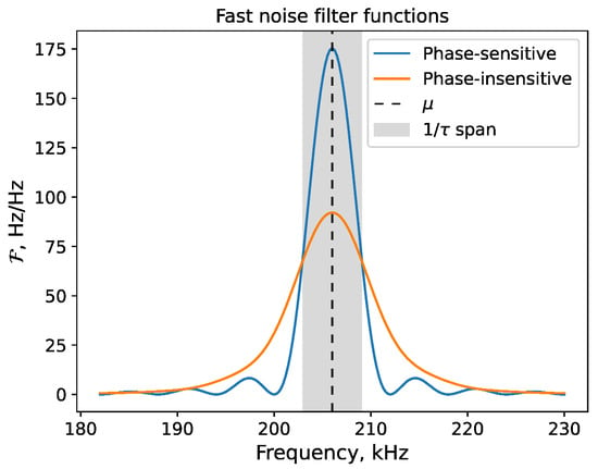
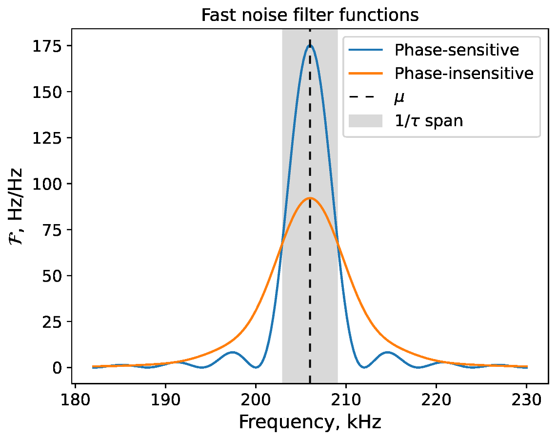
Based on the reasons listed earlier, the peak positions of the filter functions of the fast noise for both configurations should not differ much. This assumption is confirmed numerically; see Figure 4. The filter functions were calculated using the same parameters that were used for the numerical simulations in [24]:

Figure 4. Filter functions for fast laser phase noise, both sensitive and insensitive configurations. The dashed line represents the detuning from the carrier transition $\mu$. The width of the shaded region is $1/\tau$, where $\tau$ is the gate time. For other details of the calculation, see the main text.

• A single motional mode ${\omega }_l=2\pi ·200\mathrm{kHz}$;
• Lamb–Dicke parameter for this mode $\eta =0.15$;
• Rabi frequency (identical for both ions) $\mathsf{\Omega }=2\pi ·20\mathrm{kHz}$;
• Motional phases ${\varphi }_M^{\left(j\right)}=0$;
• Desired entanglement phase ${\chi }_0=\pi /4$;
• Gate time $\tau ={\displaystyle \frac{2\pi }{\mathsf{\Omega }\eta }}\sqrt{{\displaystyle \frac{{\chi }_0}{\pi }}}\approx 167$ μs [12];
• Carrier detuning $\mu ={\omega }_l+2\pi /\tau =2\pi ·206\mathrm{kHz}$.

We see that the peak positions for both functions coincide with the detuning $\mu$, and their widths are on the order of the inverse gate time. The filter function is slightly wider for the insensitive configuration, which can be attributed to the presence of other resonant frequencies that are close to $\mu$ and effectively “smear out” the function (see the previous discussion).

We can also obtain an estimate of the gate error for both cases, assuming the phase noise PSD changes slowly in frequency compared to the width of the filter function. In this case, $S_{\varphi }^{\left(1\right)}\left(f\right)$ can be moved out of the integral:

$$ϵ\approx S_{\varphi }^{\left(1\right)}\left(f_0\right){\displaystyle \underset{0}{\overset{+\infty }{\int }}}\mathcal{F}\left(f\right)df,$$

(74)

where $f_0$ is the peak frequency of $\mathcal{F}\left(f\right)$. For the phase-sensitive configuration, the integral of (34) can be calculated analytically in the limit $\mu \tau \gg 1$:

$${\displaystyle \underset{0}{\overset{+\infty }{\int }}}{\mathcal{F}}_{\mathrm{fast}}^{\left(\mathrm{S}\right)}\left(f\right)df\approx {\displaystyle \underset{-\infty }{\overset{+\infty }{\int }}}{\mathcal{F}}_{\mathrm{fast}}^{\left(\mathrm{S}\right)}\left(f\right)df={\displaystyle \frac{2}{5}}{\mathsf{\Omega }}^2\tau ,$$

(75)

therefore, in the phase-sensitive case:

$${ϵ}_{\mathrm{fast}}^{\left(\mathrm{S}\right)}={\displaystyle \frac{4}{5}}{S}_{\varphi }(\mu /2\pi ){\mathsf{\Omega }}^2\tau ,$$

(76)

where $S_{\varphi }\left(f\right)=S_{\varphi }^{\left(1\right)}\left(f\right)/2$ is the two-sided phase noise PSD. To calculate the integral of (46), we change the order of integration (integrating over the frequency first) and use the identity

$${\displaystyle \underset{0}{\overset{+\infty }{\int }}}\cos \left(2\pi f(t^{\prime }-t^{″})\right)df={\displaystyle \frac{1}{2}}\delta (t^{\prime }-t^{″}).$$

(77)

Assuming, as for the phase-sensitive case, a constant laser power that is uniform across the ions, we arrive at

$${\displaystyle \underset{0}{\overset{+\infty }{\int }}}{\mathcal{F}}_{\mathrm{fast}}^{\left(\mathrm{I}\right)}\left(f\right)df={\displaystyle \frac{4}{5}}{\mathsf{\Omega }}^2{\displaystyle \underset{0}{\overset{\tau }{\int }}}{\cos }^2(\mu t+{\varphi }_M^{\left(j\right)})dt.$$

(78)

Since we assume $\mu \tau \gg 1$, the squared cosine in the integral can be approximated by $1/2$, its average value. For the gate error, we obtain the expression

$${ϵ}_{\mathrm{fast}}^{\left(\mathrm{I}\right)}={\displaystyle \frac{4}{5}}{S}_{\varphi }(\mu /2\pi ){\mathsf{\Omega }}^2\tau ,$$

(79)

which is exactly the same expression as Formula (76) for the error in the phase-sensitive configuration. Thus, both laser beam geometries lead to the same gate error induced by fast noise. In the general modulation case, the approximate errors can be calculated in a similar way:

$${ϵ}_{\mathrm{fast}}^{\left(\mathrm{S}\right)}={ϵ}_{\mathrm{fast}}^{\left(\mathrm{I}\right)}\approx {\displaystyle \frac{4}{5}}{S}_{\varphi }(\mu /2\pi ){\displaystyle \underset{0}{\overset{\tau }{\int }}}{\mathsf{\Omega }}^2\left(t\right)dt,$$

(80)

where $\mathsf{\Omega }\left(t\right)$ is the envelope of the pulse function $g\left(t\right)$ (assuming the same one for both ions). Therefore, Equations (76) and (79) are applicable in this case as well, if $\mathsf{\Omega }$ is interpreted as the root mean square Rabi frequency of the pulse.

3.2. Comparison of the Rotating and Lab Frames in Terms of Error Induced by Slow Noise

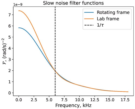
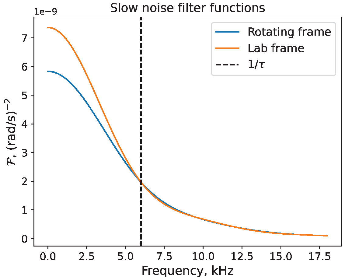
We expect the slow noise filter function to be prominent at frequencies around $\sim 1/\tau$ in both rotating and lab frames. Example functions are shown in Figure 5. The parameters chosen were identical to those used for the fast noise filter function in Figure 4.

Figure 5. Slow laser frequency noise filter functions. The dashed line represents the value $1/\tau$. Note the different units compared to ${\mathcal{F}}_{\mathrm{fast}}\left(f\right)$.

The filter functions are indeed prominent at frequencies up to approximately the inverse gate time, which also turns out to be the value after which the functions are almost the same. Therefore, the difference between the rotating and lab frames in this case is significant only up to $1/\tau$.

We can estimate the error in the case of slowly-varying frequency noise PSD for both frames in the same way as was done for fast noise: by moving the PSD out of the integral (61). As was mentioned in the introduction, the laser that performs the gate is usually stabilized by being locked to a frequency reference, such as a high-finesse Fabry–Pérot cavity [20,21,22,23], making the low-frequency noise PSD flat (aka white frequency noise) up to approximately the servo bandwidth [25]. We can then assume $S_{\omega }^{\left(1\right)}\left(f\right)$ to be constant:

$$S_{\omega }^{\left(1\right)}\left(f\right)=h_0.$$

(81)

The value $h_0$ is connected to the linewidth of the laser $\Delta \omega$ (FWHM) via the following identity [57]:

$$h_0=2\Delta \omega .$$

(82)

The integral $\int \mathcal{F}\left(f\right)df$ can be calculated using (77). Taking (82) into account, we obtain the errors as follows:

$$\begin{array}{c}{ϵ}_{\mathrm{slow}}^{\left(\mathrm{rot}\right)}\approx {\displaystyle \frac{2}{5}}\Delta \omega \tau ,\end{array}$$

(83)

$$\begin{array}{c}\begin{array}{c}\hfill {ϵ}_{\mathrm{slow}}^{\left(\mathrm{lab}\right)}\approx {\displaystyle \frac{\Delta \omega }{20}}{\displaystyle \underset{0}{\overset{\tau }{\int }}}\left\{8+{\displaystyle \sum _{s,j}}\left(1\phantom{\exp \left[-4\sum _l\left({\overline{n}}_l+{\displaystyle \frac{1}{2}}\right){\left|{\alpha }_{lj}^{\prime }\right|}^2\right]}-2\cos \left(2s_1{s}_2(\chi -{\chi }^{\prime })-2s_1{s}_2^{\prime }{\epsilon }^{\prime }\right)\right.\right.\end{array}\\ \hfill \left.\left.\times \exp \left[-4\sum _l\left({\overline{n}}_l+{\displaystyle \frac{1}{2}}\right){\left|{\alpha }_{lj}^{\prime }\right|}^2\right]\right)\right\}d{t}^{\prime }\end{array}$$

(84)

The expression (84) depends on the gate parameters. However, it is straightforward to obtain the upper bound on the error, which is independent of these parameters:

$${ϵ}_{\mathrm{slow}}^{\left(\mathrm{lab}\right)}\le {\displaystyle \frac{\Delta \omega }{20}}{\displaystyle \underset{0}{\overset{\tau }{\int }}}\left\{8+\sum _{s,j}(1+2)\right\}={\displaystyle \frac{8}{5}}\Delta \omega \tau ,$$

(85)

which has the same order of magnitude as the error in the rotating frame (83).

4. Discussion

It is important to emphasize the fact that the analysis that was done in the present work initially considered the intrinsic laser phase noise, that is, the initial noise that comes from the source of light and that is the same for all addressed ions and shifts the spin phase ${\varphi }_S$ (the noise that shifts the motional phase ${\varphi }_M$ was studied in [42]). However, it is also applicable to all ${\varphi }_S$ noise that is common to all ions. For example, it can be the optical path fluctuations in the beam before it gets physically split into individual addressing beams, electronic noise in the generators that drive the electro-optical or acousto-optical modulators of the same beam or bias magnetic field fluctuations (assuming sufficient homogeneity of this field across the chain). The noise models and their respective PSDs will differ depending on the physical source of ${\varphi }_S$ noise, but the filter functions will remain the same and can be used to describe each such source.

Furthermore, if there is noise that influences only one of the ${\varphi }_S$ phases (like optical path fluctuations in one of the individual beams or electronic noise in an individual driving signal generator), our analysis can be adapted to that scenario as well. The noise Hamiltonians (8) and (9) will lose the ion index j in the sum, which will lead to all filter functions simply losing their respective summation index j as well. The fact that the filter function for both ions is simply the sum of individual filter functions for each ion leads to the following observation: if there are two different ${\varphi }_S$ noise functions $\delta {\varphi }_j\left(t\right)$, the ${\delta }_{j{j}^{\prime }}$ terms make it so that the average gate error will only depend on the individual noise autocorrelation functions $⟨\delta \varphi \left(t^{\prime }\right)\delta \varphi \left(t^{″}\right)⟩$, even if the phase noise on the ions is partially correlated. Therefore, our analysis is directly extendable to any ${\varphi }_S$ noise of any nature as follows: the total gate error is the sum of two terms, one for each ion; each term is a convolution of the respective noise PSD (phase or frequency, for fast or slow noise, respectively) on that ion with the filter function of the gate for that ion. This is independent of any ${\varphi }_S$ fluctuation correlations between the ions.

The influence of fast laser noise on the fidelity of two-qubit gates was studied before in [24]. In the referenced work, the authors used numerical simulations to arrive at the following formula:

$$1-F=T·\mathrm{RPSD}\left(f_l\right),$$

(86)

where T is the gate time, $f_l$ is the trap secular frequency, and $\mathrm{RPSD}\left(f\right)$ is the so-called Rabi PSD, which is the laser field PSD, renormalized such that the area under the carrier peak is ${\mathsf{\Omega }}^2$. To compare this result with expressions (76) (or (79)) presented in this work, we make the following observations. First, the starting two-qubit state for the simulations in [24] was $\left|00\right.⟩$. It can be shown that if the starting state is $\left|00\right.⟩$ rather than a random one, the numerical factors $4/5$ in (76) and (79) become unity. Second, the detuning $\mu$ is assumed to be close to the motional frequency, so $S_{\varphi }\left(f_l\right)\approx S_{\varphi }(\mu /2\pi )$. Third, for small phase fluctuations, the electric field PSD of the laser at frequencies far from the carrier is proportional to the phase noise PSD [19]; therefore, $S_{\varphi }\left(f\right){\mathsf{\Omega }}^2\approx \mathrm{RPSD}\left(f\right)$, according to the definition of the latter. Combining all observations, we conclude that, under appropriate assumptions, the results obtained in this work agree with those obtained in [24].

The fast noise parts in perturbations (8) and (9) come from the carrier term in the initial Hamiltonians (2) and (5), respectively. However, this term was neglected in the noiseless evolution operator, while the noise terms themselves remained. Even though this does not seem justified at first, the errors introduced by the carrier term and the fast noise term are independent and therefore their calculation can be separated into two distinct problems. The argument is based on the same discussion that we made before when considering slow noise originating from uncorrelated sources. The fidelity in the presence of both systematic and stochastic errors can be represented in the form (69), where $\widehat{Q}$ is the systematic error introduced by the carrier term. The cross terms in this case will be linear in the fluctuation; therefore, they cancel out in the mean error. This means that the total error with a systematic and stochastic source is the sum of two errors from each source separately. Note that the same is true for the case of several uncorrelated stochastic error sources, such as motional frequency drifts or magnetic field instability mentioned before. Furthermore, the systematic error operator $\widehat{Q}$ can be any deterministic operator that represents the difference between the ideal noiseless evolution operator (17) and its desired action at the end of the gate $e^{i{\chi }_0{\sigma }_{\phi }^{\left(1\right)}{\sigma }_{\phi }^{\left(2\right)}}$. Any deviation of the entanglement phase $\chi \left(\tau \right)$ from ${\chi }_0$ and the displacement parameters ${\alpha }_{lj}\left(\tau \right)$ from zero can be incorporated into $\widehat{Q}$ with their contribution calculated separately, while the stochastic error can be evaluated using the desired dynamics $\chi \left(t\right),{\alpha }_{lj}\left(t\right)$, for which $\chi \left(\tau \right)={\chi }_0,{\alpha }_{lj}\left(\tau \right)=0$.

The difference between the rotating and the lab frame for the slow noise can be explained in the following way. In the rotating frame that is in phase with the laser (which ${\widehat{U}}_R$ is an example of), the ideal MS gate Hamiltonian, as we have shown above, will be the same as the one in the non-rotating lab frame. Phase noise comes only as an additional ${\sigma }_z$ term. The same is true for single-qubit gates. Therefore, if all gates in the quantum circuit are performed with the same laser source, the rotating frame will be the same for the entire evolution of the system, so it is possible to transition into this frame in the beginning of the circuit and move back into the lab frame once the whole circuit is finished. If the gate unitaries in the rotating frame are ${\widehat{U}}_1,{\widehat{U}}_2,\dots ,{\widehat{U}}_N$, then the total evolution operator in the lab frame will be

$${\widehat{U}}_{\mathrm{lab}}={\widehat{U}}_R^{†}\left(T_N\right){\widehat{U}}_N{\widehat{U}}_{N-1}\dots {\widehat{U}}_1,$$

(87)

where $T_N$ is the total evolution time after N gates, and we assume ${\widehat{U}}_R\left(0\right)$ is the identity. This means that in this case, the additional error due to rotation can be ignored and accounted for separately at the end, so using the rotating frame filter function (62) makes more sense. Furthermore, the rotating frame is suitable for describing other ${\sigma }_z$-type noises that are not correlated with the laser phase noise. A common example is magnetic field fluctuations, which affect the qubit frequency directly.

A different effect takes place when each gate is performed with a separate source uncorrelated with the rest. In this case, we use an equivalent representation of (87) that is the product of individual evolution operators in the lab frame:

$$\begin{array}{c}{\widehat{U}}_{\mathrm{lab}}=\left[{\widehat{U}}_R^{†}\left(T_N\right){\widehat{U}}_N{\widehat{U}}_R\left(T_{N-1}\right)\right]\hfill \\ \hfill \times \left[{\widehat{U}}_R^{†}\left(T_{N-1}\right){\widehat{U}}_{N-1}{\widehat{U}}_R\left(T_{N-2}\right)\right]\dots \left[{\widehat{U}}_R^{†}\left(T_1\right){\widehat{U}}_1{\widehat{U}}_R\left(0\right)\right]\hfill \\ \hfill ={\widehat{U}}_N^{\left(\mathrm{lab}\right)}{\widehat{U}}_{N-1}^{\left(\mathrm{lab}\right)}\dots {\widehat{U}}_1^{\left(\mathrm{lab}\right)},\end{array}$$

(88)

where

$${\widehat{U}}_n^{\left(\mathrm{lab}\right)}={\widehat{U}}_R^{†}\left(T_n\right){\widehat{U}}_n{\widehat{U}}_R\left(T_{n-1}\right).$$

(89)

In this picture, each individual operator gives its own evolution and error due to rotation. If each gate is performed by an independent source uncorrelated with the rest, then the rotation error must be accounted for in each gate separately, in which case the lab frame filter function (73) is the correct one. If there is only one gate in the circuit, both representations become identical, so the rotation error at the end of the gate cannot be separated from the error accumulated during the gate, and the function (73) will be the correct one in this case as well.

Summing up, we list the use cases for both filter functions as follows:

• Rotating frame
  • Evaluating the error of the MS gate in a multi-gate circuit implemented with the same laser source;
  • Investigating other ${\sigma }_z$-type noise sources, such as magnetic field fluctuations.
• Lab frame
  • Measuring the error of a single MS gate;
  • Measuring the error of one MS gate in a multi-gate circuit implemented with different uncorrelated sources.

Overall, despite these differences, the error estimates in both cases have been shown to be of the same order, so the universal approximation

$${ϵ}_{\mathrm{slow}}\sim \Delta \omega \tau$$

(90)

is acceptable in most cases.

The validity of the white-noise approximation that has been used for the simplified slow noise error estimate has an important caveat. Below very low frequencies (100 Hz and lower) the noise is dominated by $1/f$ noise, as was pointed out in the introduction. Strictly speaking, the convolution integral will diverge. However, this integral only diverges for an infinite measurement time. For a finite measurement time $T_0$, the error will be

$${ϵ}_T={\displaystyle \underset{1/T_0}{\overset{+\infty }{\int }}}{S}_{\omega }\left(f\right)\mathcal{F}\left(f\right)df.$$

(91)

Afterwards we will take into account the fact that for modern cavity-locked lasers the cutoff frequency $f_0$ between the white noise and $1/f$ noise is $10÷100$ Hz [31,32], which is much smaller than the width of the filter function $\sim 1/\tau$. Therefore, the integral can be divided into intervals, before and after $f_0$:

$${ϵ}_T={\displaystyle \underset{1/T_0}{\overset{f_0}{\int }}}{S}_{\omega }\left(f\right)\mathcal{F}\left(f\right)df+{\displaystyle \underset{f_0}{\overset{+\infty }{\int }}}{S}_{\omega }\left(f\right)\mathcal{F}\left(f\right)df\approx \mathcal{F}\left(0\right){\displaystyle \underset{1/T_0}{\overset{f_0}{\int }}}{S}_{\omega }\left(f\right)df+h_0{\displaystyle \underset{0}{\overset{+\infty }{\int }}}\mathcal{F}\left(f\right)df.$$

(92)

The second term is the error from the white noise approximation that was calculated before. The integral in the first term is the mean squared frequency deviation [19]. Therefore, for the error induced by a low-frequency $1/f$-type noise component, we get

$${ϵ}_{\mathrm{low}}\approx {\mathcal{F}}_{\mathrm{slow}}\left(0\right)⟨\delta {\omega }^2⟩,$$

(93)

where $\delta {\omega }^2$ is the squared frequency deviation. Physically, this result can be understood as follows. The low-noise component is only prevalent at times much longer than the gate time. Therefore, during the gate, the laser spectrum will behave like a narrow line that has the linewidth $\Delta \omega$ and is shifted by a constant $\delta \omega$. Thus, we can treat this constant shift as a noise that has a delta-like spectrum $S_{\omega }\left(f\right)=\delta {\omega }^2\delta \left(f\right)$ during the gate. Then the convolution with the same filter function ${\mathcal{F}}_{\mathrm{slow}}$ will yield the formula above. The averaging time $T_0$ depends on the design of the experiment and should take the value that makes the most sense in each specific case. For example, this can be the total duration of an uninterrupted experimental sequence, where multiple runs of the same quantum circuit are executed without intermittent re-calibrations.

To summarize our findings, we estimate some experimental requirements that should be put onto the laser system for it to be able to perform useful quantum computation. The widely accepted error value for error correction to begin offering an advantage is around ${10}^{-3}$ [58,59]. We take the same gate parameters that we used to plot the filter functions, namely: gate time $\tau =167$ μs, Rabi frequency $\mathsf{\Omega }=2\pi ·20\mathrm{kHz}$. For this set of parameters, we obtain the following:

• Phase noise PSD at $\mu /2\pi$$S_{\varphi }(\mu /2\pi )<-93\mathrm{dBc}/\mathrm{Hz}$;
• Laser linewidth $\Delta \omega <2\mathrm{Hz}$;
• Central frequency deviation $\delta \omega <65\mathrm{Hz}$.

These characteristics are achievable in practice, but are quite demanding. They require long-term stability of the cavity (both thermal and mechanical), as well as a sufficiently low Schawlow–Townes white noise floor, which motivates the use of solid-state lasers over diodes. Furthermore, a −93 dBc/Hz level of noise at the detuning can only be realized using auxiliary techniques, such as implementing a filtering cavity [60,61] or injection locking [60,62].

References

- AbuGhanem, M. IBM quantum computers: Evolution, performance, and future directions: M. AbuGhanem. J. Supercomput. 2025, 81, 687. [Google Scholar] [CrossRef] [Scilit]
- Acharya, R.; Abanin, D.A.; Aghababaie-Beni, L.; Aleiner, I.; Andersen, T.I.; Ansmann, M.; Arute, F.; Arya, K.; Asfaw, A.; Astrakhantsev, N.; et al. Quantum error correction below the surface code threshold. Nature 2024, 638, 920–926. [Google Scholar] [CrossRef] [Scilit] [PubMed]
- Ransford, A.; Allman, M.; Arkinstall, J.; Campora, J., III; Cooper, S.F.; Delaney, R.D.; Dreiling, J.M.; Estey, B.; Figgatt, C.; Hall, A.; et al. Helios: A 98-qubit trapped-ion quantum computer. arXiv 2025, arXiv:2511.05465. [Google Scholar]
- Nielsen, M.A.; Chuang, I.L. Quantum Computation and Quantum Information: 10th Anniversary Edition; Cambridge University Press: Cambridge, UK, 2010. [Google Scholar]
- Cai, Z.; Babbush, R.; Benjamin, S.C.; Endo, S.; Huggins, W.J.; Li, Y.; McClean, J.R.; O’Brien, T.E. Quantum error mitigation. Rev. Mod. Phys. 2023, 95, 045005. [Google Scholar] [CrossRef] [Scilit]
- Löschnauer, C.; Mosca Toba, J.; Hughes, A.; King, S.; Weber, M.; Srinivas, R.; Matt, R.; Nourshargh, R.; Allcock, D.; Ballance, C.; et al. Scalable, High-Fidelity All-Electronic Control of Trapped-Ion Qubits. PRX Quantum 2025, 6, 040313. [Google Scholar] [CrossRef] [Scilit]
- Quantinuum System H2-2 Benchmarks. 2025. Available online: https://docs.quantinuum.com/systems/user_guide/hardware_user_guide/benchmarks/system_benchmarks.html (accessed on 28 July 2026).
- Kielpinski, D.; Monroe, C.; Wineland, D.J. Architecture for a large-scale ion-trap quantum computer. Nature 2002, 417, 709–711. [Google Scholar] [CrossRef] [Scilit] [PubMed]
- Pino, J.M.; Dreiling, J.M.; Figgatt, C.; Gaebler, J.P.; Moses, S.A.; Allman, M.; Baldwin, C.; Foss-Feig, M.; Hayes, D.; Mayer, K.; et al. Demonstration of the trapped-ion quantum CCD computer architecture. Nature 2021, 592, 209–213. [Google Scholar] [CrossRef] [Scilit] [PubMed]
- Moses, S.; Baldwin, C.; Allman, M.; Ancona, R.; Ascarrunz, L.; Barnes, C.; Bartolotta, J.; Bjork, B.; Blanchard, P.; Bohn, M.; et al. A Race-Track Trapped-Ion Quantum Processor. Phys. Rev. X 2023, 13, 041052. [Google Scholar] [CrossRef] [Scilit]
- Sørensen, A.; Mølmer, K. Quantum Computation with Ions in Thermal Motion. Phys. Rev. Lett. 1999, 82, 1971–1974. [Google Scholar] [CrossRef] [Scilit]
- Sørensen, A.; Mølmer, K. Entanglement and quantum computation with ions in thermal motion. Phys. Rev. A 2000, 62, 022311. [Google Scholar] [CrossRef] [Scilit]
- Schäfer, V.M.; Ballance, C.J.; Thirumalai, K.; Stephenson, L.J.; Ballance, T.G.; Steane, A.M.; Lucas, D.M. Fast quantum logic gates with trapped-ion qubits. Nature 2018, 555, 75–78. [Google Scholar] [CrossRef] [Scilit] [PubMed]
- Hughes, A.; Srinivas, R.; Löschnauer, C.; Knaack, H.; Matt, R.; Ballance, C.; Malinowski, M.; Harty, T.; Sutherland, R. Trapped-ion two-qubit gates with >99.99% fidelity without ground-state cooling. arXiv 2025, arXiv:2510.17286. [Google Scholar]
- Debnath, S.; Linke, N.M.; Figgatt, C.; Landsman, K.A.; Wright, K.; Monroe, C. Demonstration of a small programmable quantum computer with atomic qubits. Nature 2016, 536, 63–66. [Google Scholar] [CrossRef] [Scilit] [PubMed]
- Chen, J.S.; Nielsen, E.; Ebert, M.; Inlek, V.; Wright, K.; Chaplin, V.; Maksymov, A.; Páez, E.; Poudel, A.; Maunz, P.; et al. Benchmarking a trapped-ion quantum computer with 30 qubits. Quantum 2024, 8, 1516. [Google Scholar] [CrossRef] [Scilit]
- Ospelkaus, C.; Warring, U.; Colombe, Y.; Brown, K.R.; Amini, J.M.; Leibfried, D.; Wineland, D.J. Microwave quantum logic gates for trapped ions. Nature 2011, 476, 181–184. [Google Scholar] [CrossRef] [Scilit] [PubMed]
- Srinivas, R.; Burd, S.C.; Knaack, H.M.; Sutherland, R.T.; Kwiatkowski, A.; Glancy, S.; Knill, E.; Wineland, D.J.; Leibfried, D.; Wilson, A.C.; et al. High-fidelity laser-free universal control of trapped ion qubits. Nature 2021, 597, 209–213. [Google Scholar] [CrossRef] [Scilit] [PubMed]
- Riehle, F. Frequency Standards: Basics and Applications; John Wiley & Sons: Hoboken, NJ, USA, 2006. [Google Scholar]
- Kolachevsky, N.; Alnis, J.; Parthey, C.G.; Matveev, A.; Landig, R.; Hänsch, T. Low phase noise diode laser oscillator for 1S–2S spectroscopy in atomic hydrogen. Opt. Lett. 2011, 36, 4299–4301. [Google Scholar] [CrossRef] [Scilit] [PubMed]
- Alnis, J.; Matveev, A.; Kolachevsky, N.; Udem, T.; Hänsch, T.W. Subhertz linewidth diode lasers by stabilization to vibrationally and thermally compensated ultralow-expansion glass Fabry-Pérot cavities. Phys. Rev. A 2008, 77, 053809. [Google Scholar] [CrossRef] [Scilit]
- Schmid, F.; Weitenberg, J.; Hänsch, T.W.; Udem, T.; Ozawa, A. Simple phase noise measurement scheme for cavity-stabilized laser systems. Opt. Lett. 2019, 44, 2709–2712. [Google Scholar] [CrossRef] [Scilit]
- Zalivako, I.; Semerikov, I.; Borisenko, A.; Aksenov, M.; Vishnyakov, P.; Sidorov, P.; Semenin, N.; Golovizin, A.; Khabarova, K.; Kolachevsky, N. Compact ultrastable laser system for spectroscopy of 2S1/2 → 2D3/2 quadrupole transition in 171Yb+ ion. Quantum Electron. 2020, 50, 850. [Google Scholar] [CrossRef] [Scilit]
- Nakav, H.; Finkelstein, R.; Peleg, L.; Akerman, N.; Ozeri, R. Effect of fast noise on the fidelity of trapped-ion quantum gates. Phys. Rev. A 2023, 107, 042622. [Google Scholar] [CrossRef] [Scilit]
- Day, M.L.; Low, P.J.; White, B.; Islam, R.; Senko, C. Limits on atomic qubit control from laser noise. npj Quantum Inf. 2022, 8, 72. [Google Scholar] [CrossRef] [Scilit]
- Lu, H.; Su, J.; Xie, C.; Peng, K. Experimental investigation about influences of longitudinal-mode structure of pumping source on a Ti: Sapphire laser. Opt. Express 2011, 19, 1344–1353. [Google Scholar] [CrossRef] [Scilit] [PubMed]
- Zhang, W.N.; Li, C.; Mo, S.P.; Yang, C.S.; Feng, Z.M.; Xu, S.H.; Shen, S.X.; Peng, M.Y.; Zhang, Q.Y.; Yang, Z.M. A compact low noise single frequency linearly polarized DBR fiber laser at 1550 nm. Chin. Phys. Lett. 2012, 29, 084205. [Google Scholar] [CrossRef] [Scilit]
- Galzerano, G.; Laporta, P.; Bonelli, L.; Toncelli, A.; Tonelli, M. Single-frequency diode-pumped Yb: KYF4 laser around 1030 nm. Opt. Express 2007, 15, 3257–3264. [Google Scholar] [CrossRef] [Scilit] [PubMed]
- Numata, K.; Kemery, A.; Camp, J. Thermal-noise limit in the frequency stabilization of lasers with rigid cavities. Phys. Rev. Lett. 2004, 93, 250602. [Google Scholar] [CrossRef] [Scilit] [PubMed]
- Kessler, T.; Legero, T.; Sterr, U. Thermal noise in optical cavities revisited. J. Opt. Soc. Am. B 2011, 29, 178–184. [Google Scholar] [CrossRef] [Scilit]
- Milani, G.; Rauf, B.; Barbieri, P.; Bregolin, F.; Pizzocaro, M.; Thoumany, P.; Levi, F.; Calonico, D. Multiple wavelength stabilization on a single optical cavity using the offset sideband locking technique. Opt. Lett. 2017, 42, 1970–1973. [Google Scholar] [CrossRef] [Scilit] [PubMed]
- Westergaard, P.G. Strontium Optical Lattice Clock: In Quest of the Ultimate Performance. Ph.D. Thesis, Laboratoire des Systemes de Reference Temps-Espace du Lab, National de Metrologie et d’Essais, Paris, France, 2010. [Google Scholar]
- Lidar, D.A.; Chuang, I.L.; Whaley, K.B. Decoherence-Free Subspaces for Quantum Computation. Phys. Rev. Lett. 1998, 81, 2594–2597. [Google Scholar] [CrossRef] [Scilit]
- Barenco, A.; Berthiaume, A.; Deutsch, D.; Ekert, A.; Jozsa, R.; Macchiavello, C. Stabilization of quantum computations by symmetrization. SIAM J. Comput. 1997, 26, 1541–1557. [Google Scholar] [CrossRef] [Scilit]
- Zanardi, P.; Rasetti, M. Noiseless Quantum Codes. Phys. Rev. Lett. 1997, 79, 3306–3309. [Google Scholar] [CrossRef] [Scilit]
- Zanardi, P. Stabilizing quantum information. Phys. Rev. A 2000, 63, 012301. [Google Scholar] [CrossRef] [Scilit]
- Duan, L.M.; Guo, G.C. Preserving Coherence in Quantum Computation by Pairing Quantum Bits. Phys. Rev. Lett. 1997, 79, 1953–1956. [Google Scholar] [CrossRef] [Scilit]
- Ban, M. Photon-echo technique for reducing the decoherence of a quantum bit. J. Mod. Opt. 1998, 45, 2315–2325. [Google Scholar] [CrossRef] [Scilit]
- Viola, L.; Knill, E.; Lloyd, S. Dynamical Decoupling of Open Quantum Systems. Phys. Rev. Lett. 1999, 82, 2417–2421. [Google Scholar] [CrossRef] [Scilit]
- Manovitz, T.; Rotem, A.; Shaniv, R.; Cohen, I.; Shapira, Y.; Akerman, N.; Retzker, A.; Ozeri, R. Fast Dynamical Decoupling of the Mølmer-Sørensen Entangling Gate. Phys. Rev. Lett. 2017, 119, 220505. [Google Scholar] [CrossRef] [Scilit] [PubMed]
- Zalivako, I.V.; Borisenko, A.S.; Semerikov, I.A.; Korolkov, A.E.; Sidorov, P.L.; Galstyan, K.P.; Semenin, N.V.; Smirnov, V.N.; Aksenov, M.D.; Fedorov, A.K.; et al. Continuous dynamical decoupling of optical 171Yb+ qudits with radiofrequency fields. Front. Quantum Sci. Technol. 2023, 2, 1228208. [Google Scholar] [CrossRef] [Scilit]
- Kang, M.; Wang, Y.; Fang, C.; Zhang, B.; Khosravani, O.; Kim, J.; Brown, K.R. Designing Filter Functions of Frequency-Modulated Pulses for High-Fidelity Two-Qubit Gates in Ion Chains. Phys. Rev. Appl. 2023, 19, 014014. [Google Scholar] [CrossRef] [Scilit]
- Lee, P.J.; Brickman, K.A.; Deslauriers, L.; Haljan, P.C.; Duan, L.M.; Monroe, C. Phase control of trapped ion quantum gates. J. Opt. B Quantum Semiclass. Opt. 2005, 7, S371. [Google Scholar] [CrossRef] [Scilit]
- Leibfried, D.; Blatt, R.; Monroe, C.; Wineland, D. Quantum dynamics of single trapped ions. Rev. Mod. Phys. 2003, 75, 281–324. [Google Scholar] [CrossRef] [Scilit]
- Aksenov, M.A.; Zalivako, I.V.; Semerikov, I.A.; Borisenko, A.S.; Semenin, N.V.; Sidorov, P.L.; Fedorov, A.K.; Khabarova, K.Y.; Kolachevsky, N.N. Realizing quantum gates with optically addressable. Phys. Rev. A 2023, 107, 052612. [Google Scholar] [CrossRef] [Scilit]
- Zalivako, I.V.; Nikolaeva, A.S.; Borisenko, A.S.; Korolkov, A.E.; Sidorov, P.L.; Galstyan, K.P.; Semenin, N.V.; Smirnov, V.N.; Aksenov, M.A.; Makushin, K.M.; et al. Towards a Multiqudit Quantum Processor Based on a 171Yb+ Ion String: Realizing Basic Quantum Algorithms. Quantum Rep. 2025, 7, 19. [Google Scholar] [CrossRef] [Scilit]
- Anikin, E.; Chuchalin, A.; Morozov, N.; Lakhmanskaya, O.; Lakhmanskiy, K. Fast Mølmer-Sørensen gates in trapped-ion quantum processors with compensated carrier transition. Phys. Rev. Appl. 2025, 24, 014044. [Google Scholar] [CrossRef] [Scilit]
- Kirchmair, G.; Benhelm, J.; Zähringer, F.; Gerritsma, R.; Roos, C.F.; Blatt, R. Deterministic entanglement of ions in thermal states of motion. New J. Phys. 2009, 11, 023002. [Google Scholar] [CrossRef] [Scilit]
- Roos, C.F. Ion trap quantum gates with amplitude-modulated laser beams. New J. Phys. 2008, 10, 013002. [Google Scholar] [CrossRef] [Scilit]
- Blümel, R.; Grzesiak, N.; Pisenti, N.; Wright, K.; Nam, Y. Power-optimal, stabilized entangling gate between trapped-ion qubits. npj Quantum Inf. 2021, 7, 147. [Google Scholar] [CrossRef] [Scilit]
- Weber, M.A.; Gely, M.F.; Hanley, R.K.; Harty, T.P.; Leu, A.D.; Löschnauer, C.M.; Nadlinger, D.P.; Lucas, D.M. Robust and Fast Microwave-Driven Quantum Logic for Trapped-Ion Qubits. Phys. Rev. A 2024, 110, L010601. [Google Scholar] [CrossRef] [Scilit]
- Zhu, S.L.; Monroe, C.; Duan, L.M. Arbitrary-Speed Quantum Gates within Large Ion Crystals through Minimum Control of Laser Beams. Europhys. Lett. 2006, 73, 485. [Google Scholar] [CrossRef] [Scilit]
- Milne, A.R.; Edmunds, C.L.; Hempel, C.; Roy, F.; Mavadia, S.; Biercuk, M.J. Phase-Modulated Entangling Gates Robust to Static and Time-Varying Errors. Phys. Rev. Appl. 2020, 13, 024022. [Google Scholar] [CrossRef] [Scilit]
- Choi, T.; Debnath, S.; Manning, T.A.; Figgatt, C.; Gong, Z.X.; Duan, L.M.; Monroe, C. Optimal Quantum Control of Multimode Couplings between Trapped Ion Qubits for Scalable Entanglement. Phys. Rev. Lett. 2014, 112, 190502. [Google Scholar] [CrossRef] [Scilit] [PubMed]
- Shapira, Y.; Shaniv, R.; Manovitz, T.; Akerman, N.; Peleg, L.; Gazit, L.; Ozeri, R.; Stern, A. Theory of Robust Multiqubit Nonadiabatic Gates for Trapped Ions. Phys. Rev. A 2020, 101, 032330. [Google Scholar] [CrossRef] [Scilit]
- Abramowitz, M.; Stegun, I.A. Handbook of Mathematical Functions: With Formulas, Graphs, and Mathematical Tables; Courier Corporation: North Chelmsford, MA, USA, 1965. [Google Scholar]
- Di Domenico, G.; Schilt, S.; Thomann, P. Simple approach to the relation between laser frequency noise and laser line shape. Appl. Opt. 2010, 49, 4801–4807. [Google Scholar] [CrossRef] [Scilit] [PubMed]
- Ryan-Anderson, C.; Bohnet, J.G.; Lee, K.; Gresh, D.; Hankin, A.; Gaebler, J.P.; Francois, D.; Chernoguzov, A.; Lucchetti, D.; Brown, N.C.; et al. Realization of real-time fault-tolerant quantum error correction. Phys. Rev. X 2021, 11, 041058. [Google Scholar] [CrossRef] [Scilit]
- Bluvstein, D.; Evered, S.J.; Geim, A.A.; Li, S.H.; Zhou, H.; Manovitz, T.; Ebadi, S.; Cain, M.; Kalinowski, M.; Hangleiter, D.; et al. Logical quantum processor based on reconfigurable atom arrays. Nature 2024, 626, 58–65. [Google Scholar] [CrossRef] [Scilit] [PubMed]
- Krinner, L.; Dietze, K.; Pelzer, L.; Spethmann, N.; Schmidt, P.O. Low phase noise cavity transmission self-injection locked diode laser system for atomic physics experiments. Opt. Express 2024, 32, 15912–15922. [Google Scholar] [CrossRef] [Scilit] [PubMed]
- Semenin, N.; Zalivako, I.; Smirnov, V.; Semerikov, I.; Borisenko, A.; Korolkov, A.; Sidorov, P.; Galstyan, K.; Khabarova, K.; Kolachevsky, N. Improved laser-filtering scheme for quantum manipulations with the 171 Yb+ optical qubit. Phys. Rev. Appl. 2025, 23, 034080. [Google Scholar] [CrossRef] [Scilit]
- Galstyan, K.; Zalivako, I.; Kryuchkov, D.; Kolachevsky, N. Injection locking for spectral filtering of the addressing laser for optical qubits in 171yb+ ions. Radiophys. Quantum Electron. 2024, 67, 13–22. [Google Scholar] [CrossRef] [Scilit]
- Nielsen, M.A. A simple formula for the average gate fidelity of a quantum dynamical operation. Phys. Lett. A 2002, 303, 249–252. [Google Scholar] [CrossRef] [Scilit]
- Wu, Y. Noise analysis for high-fidelity quantum entangling gates in an anharmonic linear Paul trap. Phys. Rev. A 2018, 97, 062325. [Google Scholar] [CrossRef] [Scilit]
Disclaimer/Publisher’s Note: The statements, opinions and data contained in all publications are solely those of the individual author(s) and contributor(s) and not of MDPI and/or the editor(s). MDPI and/or the editor(s) disclaim responsibility for any injury to people or property resulting from any ideas, methods, instructions or products referred to in the content. |
© 2026 by the authors. Licensee MDPI, Basel, Switzerland. This article is an open access article distributed under the terms and conditions of the Creative Commons Attribution (CC BY) license.