Numerical Simulation of Ice Accretion and Galloping Analysis of Auxiliary Conductors in Electrified Railway Overhead Contact Systems

Abstract

Ice accretion and wind-induced galloping of auxiliary conductors threaten the operational reliability of electrified railway overhead contact systems. This study develops an integrated numerical framework for simulating ice-shape evolution and galloping responses of a 20.6-mm-diameter auxiliary conductor. Airflow and supercooled droplet trajectories are calculated using the SST k–ω model and the Lagrangian discrete-phase method, respectively. The Makkonen icing theory and Messinger heat-balance model are coupled to predict droplet collection, freezing, and ice growth. The effects of wind speed, droplet median volume diameter, liquid water content, and ambient temperature on ice morphology are investigated. A two-dimensional, two-degree-of-freedom fluid–structure interaction model is further established using an overset mesh and user-defined functions and validated through low-speed wind-tunnel tests. Results show that ice initially forms at the windward leading edge and extends toward both sides. Wind speed increases ice thickness and coverage, droplet size mainly enlarges the icing region, liquid water content promotes ice growth, and lower temperature concentrates ice on the windward surface. Unlike the decaying response of the bare conductor, the crescent-iced conductor exhibits sustained periodic galloping with amplitudes increasing markedly with wind speed. The proposed framework supports icing-risk assessment and anti-galloping design.

1. Introduction

The overhead contact system (OCS) of electrified railways is a critical component of the traction power supply system, consisting not only of the contact suspension system (including messenger wires, contact wires, droppers, and registration assemblies) but also auxiliary conductors such as positive feeders, protective wires, return conductors, and overhead ground wires. Although these conductors do not directly participate in pantograph–contact wire current collection, their operating conditions significantly influence electrical performance, structural safety, and operational reliability [1,2,3,4]. Meanwhile, dynamic stability issues of OCS have attracted increasing attention, as various instability mechanisms, including aerodynamic instability, parametric excitation, and self-excited vibration in pantograph–catenary interaction, may lead to excessive oscillations and deteriorate system performance. Despite different physical origins, these phenomena share common characteristics of dynamic instability and oscillatory response growth.

Some electrified railway lines in China traverse alpine regions, canyon wind corridors, bridges, and areas prone to freezing rain. Under the combined effects of low temperature, high humidity, supercooled fog droplets, and sustained winds, ice forms on auxiliary conductors through airflow transport, inertial impingement, surface collection, heat transfer, and phase-change freezing [5,6]. Ice accretion alters the conductor mass per unit length, projected windward area, sag, tension, and aerodynamic characteristics. In particular, asymmetric ice accretion can destabilize the conductor aerodynamically and induce low-frequency, large-amplitude galloping under specific wind speeds and angles of attack. Such galloping increases conductor displacement and dynamic loads at suspension points and may cause fatigue damage to fittings, strand breakage, or even conductor failure, thereby threatening traction power supply reliability and train operational safety [7,8]. Therefore, investigating ice accretion and galloping responses of auxiliary conductors is of considerable engineering significance.

Research on ice accretion of overhead conductors has initially focused on estimating ice loads and mitigating icing-related hazards in transmission lines. Early studies mainly employed empirical and semi-empirical methods to evaluate equivalent ice thickness based on meteorological parameters. Makkonen et al. [9] proposed a physical icing model based on mass conservation, describing ice growth through droplet impingement, water collection, and freezing processes. This framework was further extended to characterize different atmospheric icing types, including glaze, rime, icicles, and wet snow [10,11]. With the development of computational fluid dynamics, icing studies have gradually shifted from simplified ice-load estimation toward detailed analyses of droplet impingement, heat transfer, and ice-shape evolution. Fu et al. [12] developed a dynamic icing model by coupling airflow fields, droplet trajectories, collision efficiency, and thermal processes to predict ice growth under different conditions. Niu et al. [13,14] further investigated the effects of environmental parameters and validated icing models through observations and artificial icing tests. Recent studies have mainly focused on the influence of wind speed, temperature, liquid water content, droplet size, and conductor geometry on icing characteristics. Zhang et al. [15] analyzed the effect of stranded conductor surfaces on droplet collision efficiency, while Xu et al. [16,17] investigated the influence of meteorological conditions and droplet dynamics on ice-shape evolution and collection behavior. For multi-conductor systems, shielding effects and wake interference may further modify the local airflow and droplet distribution, leading to different icing characteristics among conductors. Qing et al. [18] investigated rime-ice accretion on bundled conductors through numerical simulations and icing wind-tunnel tests, demonstrating that the icing characteristics of downstream conductors were strongly affected by conductor spacing and arrangement. Huang et al. [19] further confirmed through natural icing tests that single-conductor icing models may lead to prediction errors when applied to multi-conductor systems. These studies indicate that conductor icing is governed not only by meteorological conditions but also by conductor geometry and spatial configuration. In recent years, icing prediction based on monitoring data and machine learning methods has attracted increasing attention. Zarnani et al. [20] combined numerical weather prediction data with support vector machines for ice-growth prediction, while Sun et al. [21,22] developed data-driven methods based on wavelet analysis, extreme learning machines, and icing evolution characteristics. Chen et al. [23] further incorporated meteorological and image information to evaluate icing severity. Subsequently, Zhao et al. [24,25,26] improved icing prediction by considering failure probability, icing efficiency, and online monitoring data, respectively. Wang et al. [27,28] introduced conductor mechanical states and physical constraints into data-driven models, enhancing prediction stability and interpretability. Meanwhile, wind-induced vibration, wind deflection, and galloping remain important factors affecting conductor safety.

The dynamic stability of the pantograph–catenary system in high-speed railways has been studied to some extent both domestically and internationally. Regarding aerodynamic instability, Stickland et al. [29,30] systematically investigated the aerodynamic characteristics and mechanical damping properties of railway contact wires under cross-wind conditions, revealing the influence of aerodynamic forces and structural damping on galloping instability. Similar aerodynamic instability mechanisms have also been studied in power transmission systems. Chabart et al. [31] experimentally investigated conductor galloping through wind-tunnel tests, while Zhou et al. [32] analyzed the galloping behavior of iced bundled conductors and demonstrated the significant influence of icing-induced aerodynamic asymmetry on large-amplitude oscillations. Recently, Fan et al. [33] proposed an active anti-galloping spoiler deployment method for railway overhead contact lines, providing a new approach for suppressing aerodynamic instability. In addition to wind-induced instability, dynamic responses of railway overhead systems under complex operational excitations have been extensively studied. Song et al. [34,35] developed numerical methods for evaluating pantograph–catenary dynamic performance, including a spatial coupling model considering vehicle–track excitation and a pseudo-excitation-based response spectrum method for analyzing stochastic wind-induced responses. Sugahara et al. [36] investigated the influence of contact wire cross-sectional modification on fatigue resistance, highlighting the importance of structural optimization for improving long-term reliability. Meanwhile, intelligent methods have been increasingly introduced for condition assessment and performance prediction of railway overhead systems. Wang et al. [37] proposed a time-frequency dual-domain deep learning framework for high-speed pantograph–catenary dynamic performance prediction, while Chen et al. [38] developed an encoder–decoder-based approach for automatic defect detection of catenary systems. In addition, Amano et al. [39,40] investigated friction-induced self-excited vibration mechanisms and the influence of periodic catenary structures on vibration stability, demonstrating that sliding friction and structural periodicity may significantly affect the stability boundary and oscillatory responses. Although these instability phenomena originate from different physical mechanisms, they share common characteristics involving dynamic instability and amplification of oscillatory responses.

Overall, existing research on overhead-conductor icing has primarily focused on transmission lines, for which relatively mature frameworks have been established for icing mechanisms, ice-shape evolution, and icing-state prediction. In the railway field, however, most studies have concentrated on the contact wire. By comparison, the ice-accretion behavior of auxiliary conductors, the effects of environmental parameters, and their post-icing aerodynamic stability remain insufficiently understood. Moreover, the relationship between ice-shape evolution and galloping response has not been systematically established or adequately validated through experiments. It is therefore necessary to develop an integrated analytical framework covering environmental conditions, ice-shape evolution, and dynamic response. To address these gaps, this study considers an auxiliary conductor with a diameter of 20.6 mm in an electrified railway overhead contact system. The microscopic geometry of the stranded surface is neglected, and the conductor is simplified as a circular cross-section. First, a numerical icing model is established to calculate the surrounding airflow field, the trajectories of supercooled water droplets, and the surface impingement characteristics. The effects of wind speed, droplet median volume diameter, liquid water content, and ambient temperature on ice thickness, icing coverage, and ice-shape morphology are then investigated. Next, a two-dimensional, two-degree-of-freedom fluid–structure interaction model is developed for the iced auxiliary conductor, and the horizontal and vertical vibration responses of bare and crescent-iced conductors are compared under different wind speeds. Finally, wind-tunnel tests are conducted to measure displacement responses under various wind speeds and icing angles of attack, thereby validating the rationality of the proposed numerical model. The contribution of this study lies in extending icing and galloping analysis to railway auxiliary conductors and examining the relationship between environmental icing conditions, ice morphology, and post-icing dynamic response through combined numerical and experimental analyses.

2. Numerical Model and Method for Ice Accretion on Auxiliary Conductors

2.1. Development of the Ice Accretion Model and Computational Domain

An auxiliary conductor with a diameter D of 20.6 mm was selected as the research object. In practical railway overhead contact systems, auxiliary conductors generally have stranded surface structures, which may influence local airflow characteristics, droplet impingement distribution, and small-scale ice morphology. In this study, the stranded surface details are neglected and the conductor is modeled as a smooth circular cylinder to reduce computational complexity and focus on the dominant icing evolution and galloping characteristics. This simplification may introduce deviations in the prediction of local icing features; however, it is considered acceptable for evaluating the overall influence of environmental parameters and ice-induced aerodynamic instability. The effects of detailed stranded geometry will be further investigated in future work.

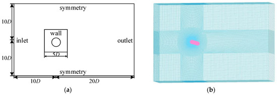
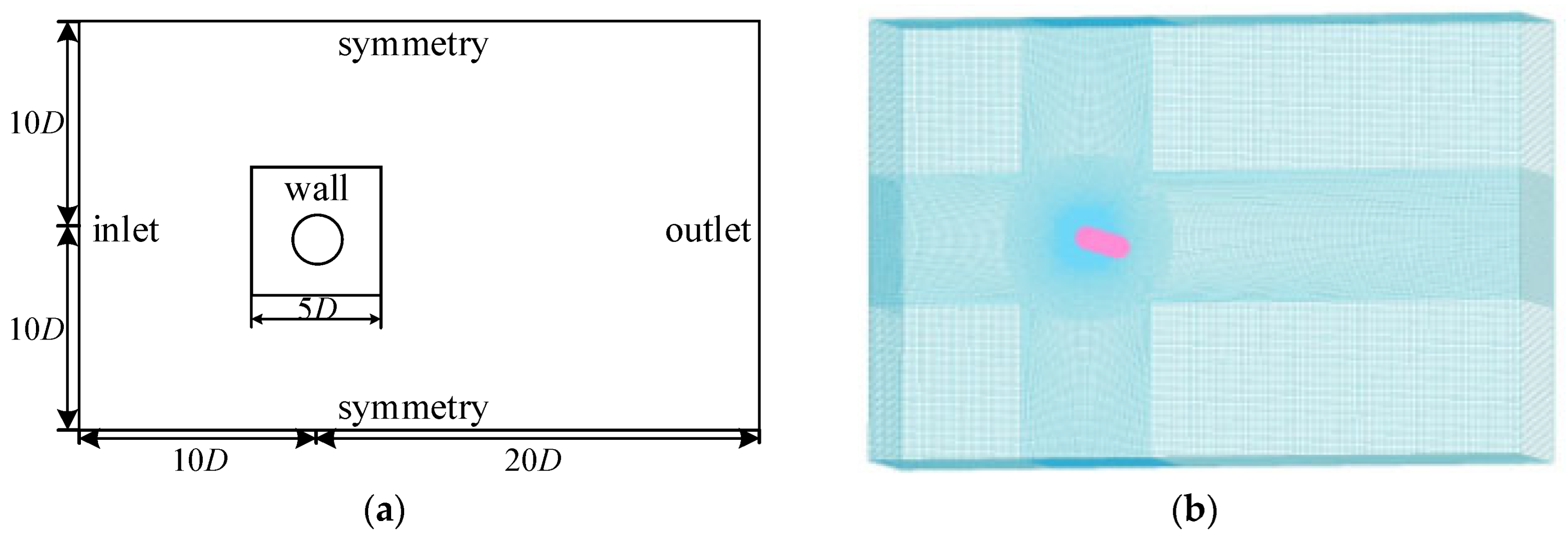
The computational domain was defined as 20D × 30D, with the conductor center located 10D downstream of the inlet and 20D upstream of the outlet. A 5D × 5D region surrounding the conductor was locally refined. The computational domain and mesh configuration are shown in Figure 1. The blue region represents the computational mesh, and the pink region represents the auxiliary conductor. The conductor length was set to 100 mm. A velocity-inlet boundary condition was applied at the left boundary, a free-outflow condition at the right boundary, and symmetry conditions at the upper and lower boundaries. A no-slip condition was imposed on the conductor surface. A pressure-based solver was employed, and the SST k–ω turbulence model was used to simulate the incompressible flow around the conductor. Pressure–velocity coupling was achieved using the SIMPLEC algorithm.

Figure 1. Computational domain and mesh configuration. (a) Computational domain and boundary conditions; (b) mesh configuration.

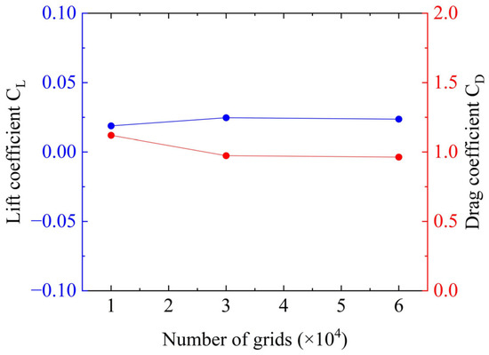
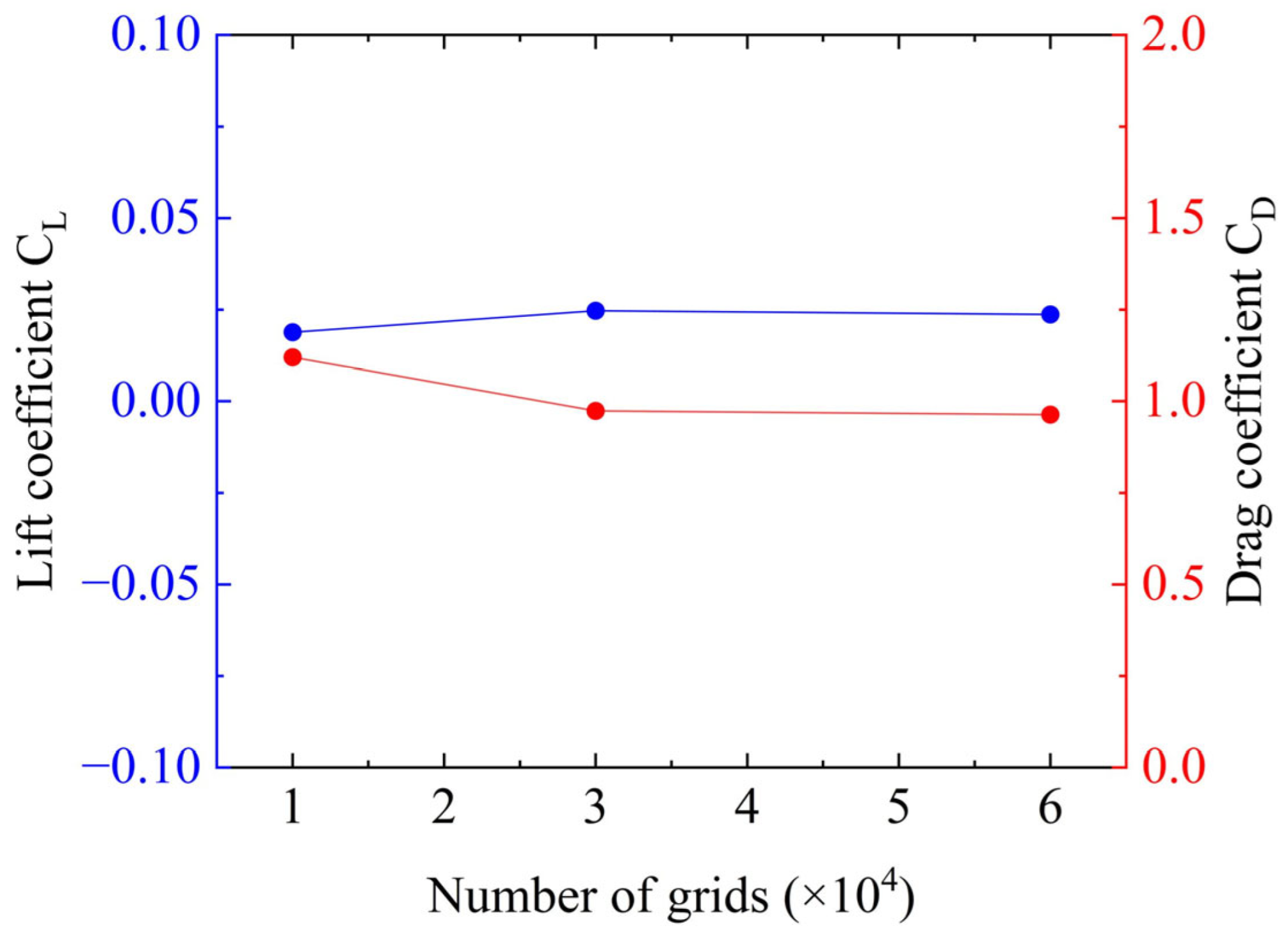
To eliminate the influence of mesh size on the computed flow-field results, numerical simulations were performed using several meshes of different resolutions, followed by a mesh-independence assessment. The lift and drag coefficients of the auxiliary conductor were calculated as the mesh density was progressively increased, as shown in Figure 2. The blue line represents the lift coefficient (C_L), and the red line represents the drag coefficient (C_D). Further mesh refinement resulted in variations of less than ±0.05 in both aerodynamic coefficients, indicating that the numerical results were only weakly sensitive to the mesh size and had essentially converged. Considering both computational accuracy and efficiency, the current mesh configuration was adopted for the subsequent simulations.

Figure 2. Mesh-independence verification.

After specifying the boundary conditions and relevant parameters, the turbulence quantities for the SST k–ω model are calculated as follows:

$$\left\{\begin{array}{c}I=0.16R{e}^{-{\displaystyle \frac{1}{8}}}\\ k=1.5{(\overline{u}I)}^2\\ w=\rho C_{\mathsf{\mu }}{k}^2/{\mu }_t\end{array}\right.,$$

(1)

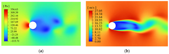
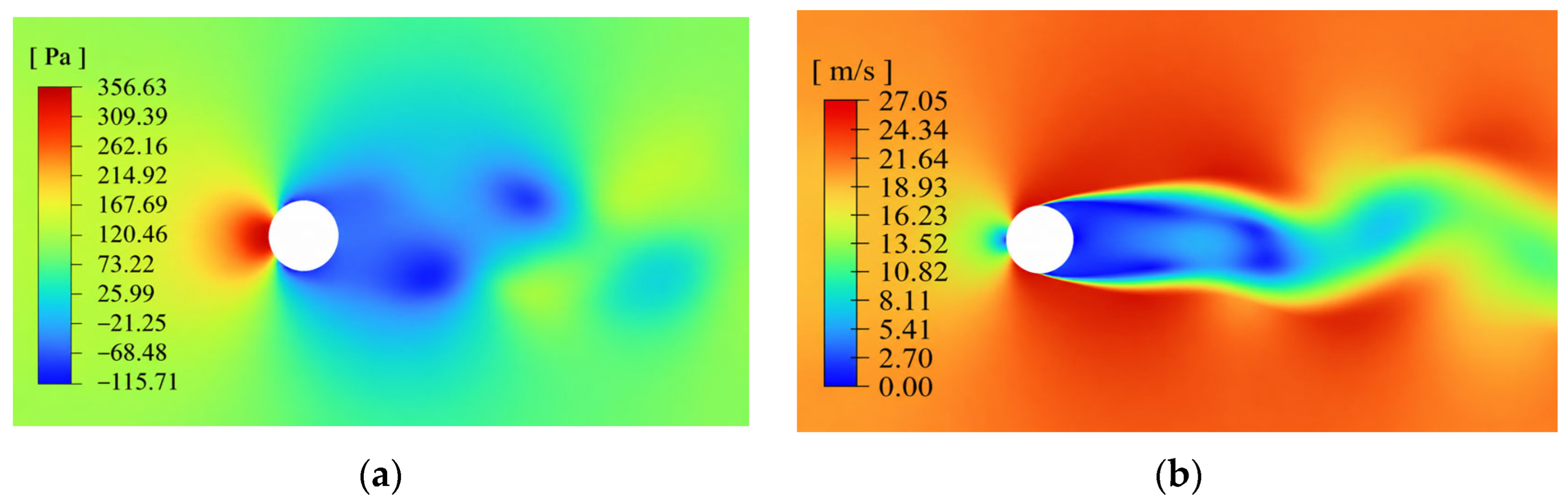
where I is the turbulence intensity, k is the turbulent kinetic energy, $Re$ is the Reynolds number, $\overline{u}$ is the mean flow velocity, w is the specific dissipation rate, $\rho$ is the fluid density, ${\mu }_t$ is the turbulent viscosity, and $C_{\mathsf{\mu }}$ is a turbulence-model constant, typically taken as 0.09. The simulation was performed at a wind speed of 5 m/s and an angle of attack of 0°. The resulting airflow-field distribution around the auxiliary conductor is shown in Figure 3.

Figure 3. Flow-field analysis of the auxiliary conductor. (a) Pressure contour; (b) velocity contour.

As shown in Figure 3, because the auxiliary conductor is simplified as a regular circular cross-section, a distinct stagnation region forms on the windward surface, where the flow velocity decreases rapidly and the pressure rises markedly, producing a localized high-pressure zone. As the airflow accelerates along the curved surface toward the upper and lower sides of the conductor, the boundary-layer velocity gradually increases, resulting in approximately symmetric low-pressure regions on both sides. After passing the conductor, the flow separates and forms a characteristic Kármán vortex street in the wake, accompanied by periodic velocity fluctuations and alternating high- and low-pressure regions. When droplets travel from left to right with the incoming flow, the highest velocities and lowest pressures occur near the upper and lower sides of the conductor, whereas the low-velocity, high-pressure stagnation region on the windward surface is more conducive to droplet impingement and retention. Overall, owing to its smooth and symmetric cross-section, the auxiliary conductor exhibits an approximately symmetric pressure and velocity distribution about the flow centerline.

2.2. Analysis of Water-Droplet Impingement on the Auxiliary Conductor Surface

Ice accretion on an auxiliary conductor is a complex physical process involving the impingement, collection, and freezing of supercooled water droplets suspended in the airflow. The Makkonen model is commonly used to investigate the characteristics and mechanisms of ice accretion and is expressed as follows:

$${\displaystyle \frac{dM}{dt}}={\alpha }_1{\alpha }_2{\alpha }_{3}v\varpi A,$$

(2)

where $v$ is the wind speed, $\varpi$ is the liquid water content of the air, and A is the effective windward area of the conductor. ${\alpha }_1$ is the collision efficiency, representing the probability that water droplets impinge on the object surface; it is related to the airflow velocity, droplet diameter, and object geometry. ${\alpha }_2$ is the collection efficiency, representing the probability that impinging droplets are retained on the surface; it is primarily affected by surface roughness and wettability. ${\alpha }_3$ is the freezing fraction, representing the proportion of collected droplets that freeze into ice; it depends mainly on the ambient temperature and the degree of droplet supercooling.

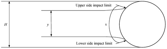
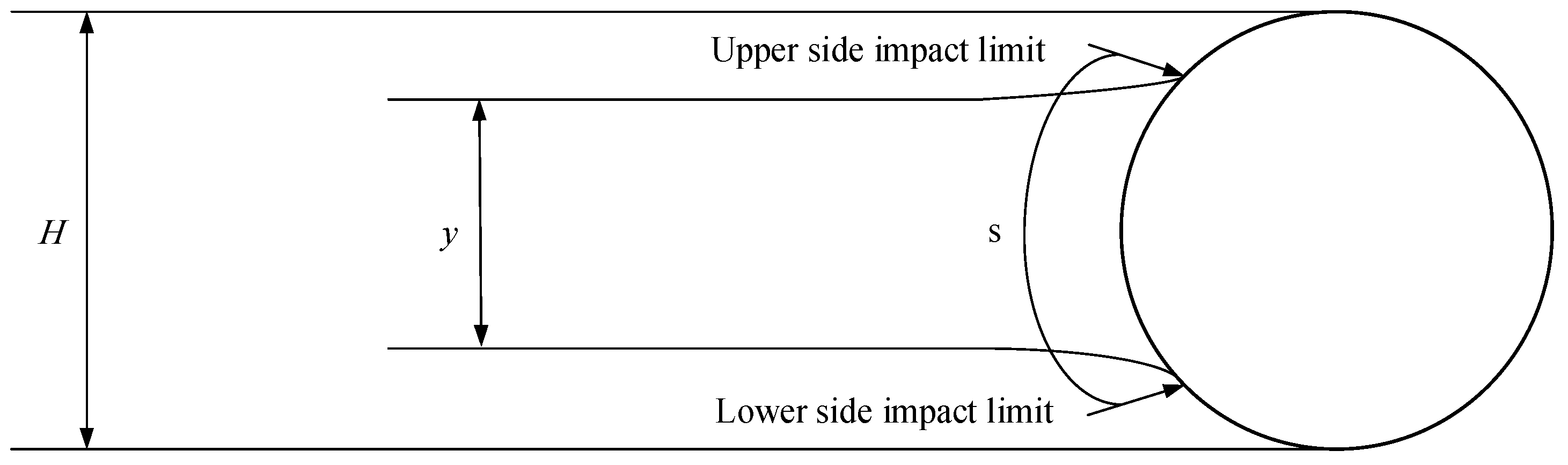
To characterize droplet impingement more clearly, the local and overall collision efficiencies are introduced. Based on the methodology reported in [41], the schematic illustration of droplet trajectories and impingement limits is presented in Figure 4. The droplets initially distributed over an upstream height H are assumed to move toward the auxiliary conductor with the incoming airflow. Due to aerodynamic deflection, most droplets bypass the conductor and follow the surrounding streamlines without impingement. Only droplets originating from the upstream interval y can eventually collide with the conductor surface. The two limiting trajectories, which are tangent to the upper and lower surfaces of the conductor, define the boundaries of the droplet impingement region. The area enclosed between these trajectories represents the effective wetted region on the conductor surface.

Figure 4. Schematic of water-droplet impingement [41].

The local collision efficiency, $\beta$, is defined as follows:

$$\beta ={\displaystyle \frac{dy}{ds}},$$

(3)

where $dy$ is the initial vertical separation between two adjacent droplet trajectories in the incoming flow, and $ds$ is the distance between the corresponding impingement points on the surface of the iced conductor. The value of $dy$ varies with the number of droplets represented by the tracked trajectories. For example, the droplet concentration is highest near the stagnation point on the left side of the conductor and gradually decreases along both sides away from the stagnation point, ultimately reaching zero at the impingement limits.

The overall collision efficiency, ${\alpha }_1$, is defined as the ratio of the actual amount of water droplets impinging on the conductor surface per unit time to the maximum possible impingement amount. The maximum possible impingement corresponds to the amount of droplets that would strike the conductor surface if their trajectories were not deflected by the airflow. Accordingly, the overall droplet collision efficiency can be expressed as follows:

$${\alpha }_1={\displaystyle \frac{y}{H}},$$

(4)

According to their definitions and governing equations, both ${\alpha }_1$ and $\beta$ are dimensionless quantities ranging from 0 to 1.

To simulate the trajectories of droplets in the airflow, a Lagrangian approach is employed to track the droplet phase. The water droplets are treated as a discrete phase, and the motion of each individual droplet is tracked [41]. Based on Newton’s second law, the governing equation for droplet motion is formulated as follows:

$$m_w{\displaystyle \frac{d^2{\overrightarrow{x}}_w}{d{t}^2}}={\overrightarrow{F}}_1+{\overrightarrow{F}}_2={\displaystyle \frac{1}{2}}{\rho }_a{A}_w{C}_d\left|{\overrightarrow{u}}_a-{\overrightarrow{u}}_w\right|({\overrightarrow{u}}_a-{\overrightarrow{u}}_w)+m_w\overrightarrow{g},$$

(5)

where $m_w$ is the droplet mass, ${\overrightarrow{x}}_w$ is the droplet displacement vector, t is the droplet travel time, ${\overrightarrow{F}}_1$ is the aerodynamic drag force acting on the droplet, $\overrightarrow{F}$ is the gravitational force acting on the droplet, ${\rho }_a$ is the air density (kg/m³), $A_w$ is the droplet frontal area (m²), $C_d$ is the droplet drag coefficient, ${\overrightarrow{u}}_a$ is the air-velocity vector, and ${\overrightarrow{u}}_w$ is the droplet-velocity vector.

The frontal area of a water droplet, $A_w$ can be calculated as follows:

$$A_w={\displaystyle \frac{4}{3}}\pi {\rho }_w{\left({\displaystyle \frac{d_w}{2}}\right)}^3={\displaystyle \frac{1}{6}}\pi {\rho }_w{d}_w^3,$$

(6)

where ${\rho }_w$ is the water-droplet density (kg/m3), and $d_w$ is the droplet diameter (m). Substituting Equation (6) into Equation (5) yields

$${\displaystyle \frac{d^2{\overrightarrow{x}}_w}{d{t}^2}}={\displaystyle \frac{18{\rho }_a{C}_d}{24{\rho }_w{d}_w}}|{\overrightarrow{u}}_a-{\overrightarrow{u}}_w|({\overrightarrow{u}}_a-{\overrightarrow{u}}_w)+\overrightarrow{g},$$

(7)

where the drag coefficient $C_d$ can be calculated as follows:

$$\left\{\begin{array}{l}{\displaystyle \frac{C_d{R}_e}{24}}=1+0.189\times R_e^{0.632},\hspace{1em}21<R_e\le 200\\ {\displaystyle \frac{C_d{R}_e}{24}}=1+0.115\times R_e^{0.802},\hspace{1em}2<R_e\le 21\\ {\displaystyle \frac{C_d{R}_e}{24}}=1+0.102\times R_e^{0.955},\hspace{1em}0.2<R_e<2\\ {\displaystyle \frac{C_d{R}_e}{24}}=1+0.197\times R_e^{0.63}+2.6\times {10}^{-4}\times R_e^{1.38},\hspace{1em}{R}_e<0.2\hspace{0.33em}\mathrm{or}\hspace{0.33em}{R}_e>200\end{array}\right.,$$

(8)

Substituting Equation (8) into Equation (7) yields

$$\left\{\begin{array}{l}{\displaystyle \frac{d{\overrightarrow{x}}_w}{dt}}={\overrightarrow{u}}_w\hfill \\ {\displaystyle \frac{d{\overrightarrow{u}}_w}{dt}}+{\displaystyle \frac{3C_d{R}_e}{4}}{\displaystyle \frac{{\mu }_a}{{\rho }_w{d}_w^2}}{\overrightarrow{u}}_w={\displaystyle \frac{3C_d{R}_e}{4}}{\displaystyle \frac{{\mu }_a}{{\rho }_w}}{\overrightarrow{u}}_a+\overrightarrow{g}\hfill \end{array}\right.,$$

(9)

By integrating Equation (9) with respect to time, the droplet velocity and displacement at each time step can be obtained, thereby determining the droplet trajectory.

2.3. Calculation of Ice Accretion on the Auxiliary Conductor Surface

Because water droplets in the atmosphere do not have a single fixed diameter but instead exhibit a complex polydisperse size distribution, the median volume diameter (MVD) is commonly adopted as a representative droplet size to simplify the calculations. The MVD characterizes the central tendency of the droplet-size distribution, thereby reducing the influence of droplet-size variability on the computational results and substantially lowering the computational complexity. When the droplet MVD is less than 50 μm, the Langmuir distribution is commonly used to describe the droplet-size spectrum. The Langmuir model is a statistical distribution model for liquid-droplet sizes. By discretizing this distribution, the proportions of droplets in different size classes can be determined, enabling more accurate simulation and prediction of conductor ice accretion. The seven specific droplet-size distributions considered in this study are listed in Table 1.

Table 1. Water drop multi-size distribution table.

Droplet Diameter/μm	Volume Fraction/%
44.4	5
34.8	10
27.4	20
20	30
14.2	20
10.4	10
6.2	5

Based on the fundamental conservation laws governing the icing process in the overhead contact system, particularly the conservation of mass and energy, the widely used icing model adopts the thermodynamic framework originally proposed by Messinger. This model can be applied to arbitrarily defined control-volume elements while ensuring the conservation of both mass and energy. For the present system, the mass- and energy-balance equations are expressed as follows:

$$M_{\mathrm{imp}}+M_{\mathrm{in}}=M_{\mathrm{eva}}+M_{\mathrm{out}}+M_{\mathrm{ice}},$$

(10)

$$q_{\mathrm{imp}}+q_{\mathrm{in}}+q_{\mathrm{air}}=q_{\mathrm{htc}}+q_{\mathrm{eva}}+q_{\mathrm{clh}}+q_{\mathrm{out}}+q_{\mathrm{ice}},$$

(11)

where $M_{\mathrm{imp}}$ is the mass of water droplets impinging on the ice layer at the control-volume surface; $M_{\mathrm{in}}$ is the mass of liquid water entering the control volume; $M_{\mathrm{eva}}$ is the mass of liquid water evaporating from the control-volume surface; $M_{\mathrm{out}}$ is the mass of liquid water leaving the control volume; $M_{\mathrm{ice}}$ is the mass of ice formed within the control volume; $q_{\mathrm{imp}}$ is the heat exchanged between the ice layer and the surrounding air; $q_{\mathrm{in}}$ is the energy carried into the control volume by external liquid water; $q_{\mathrm{air}}$ is the energy transferred by convection between the airflow and the control volume; $q_{\mathrm{htc}}$ is the energy transferred by heat conduction; $q_{\mathrm{eva}}$ is the energy removed through liquid-water evaporation; $q_{\mathrm{clh}}$ is the latent heat released during liquid-water freezing; $q_{\mathrm{out}}$ is the energy carried away by liquid water leaving the control volume; and $q_{\mathrm{ice}}$ is the energy stored in the ice within the control volume.

The calculation of the ice mass $M_{\mathrm{ice}}$ formed within the control volume requires the introduction of the freezing fraction ${\alpha }_3$. The freezing fraction is defined as the ratio of the mass of ice formed within the control volume to the total mass of liquid water entering the control volume, as expressed in Equation (12):

$${\alpha }_3={\displaystyle \frac{M_{\mathrm{ice}}}{M_{\mathrm{c}}+M_{\mathrm{i}}}},$$

(12)

After introducing the freezing fraction, the mass of ice formed, $M_{\mathrm{ice}}$, can be expressed as follows:

$$M_{\mathrm{ice}}={\alpha }_3(M_{\mathrm{c}}+M_{\mathrm{i}})$$

(13)

Once the ice mass $M_{\mathrm{ice}}$ formed within the control volume has been determined, the ice thickness h on the control-volume surface can be calculated using Equation (14) as follows:

$$h={\displaystyle \frac{M_{ice}}{{\rho }_{ice}ds}}\Delta t,$$

(14)

where ${\rho }_{ice}$ is the ice density, and $\Delta t$ is the icing step length.

2.4. Analysis of the Numerical Results

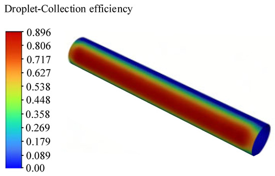
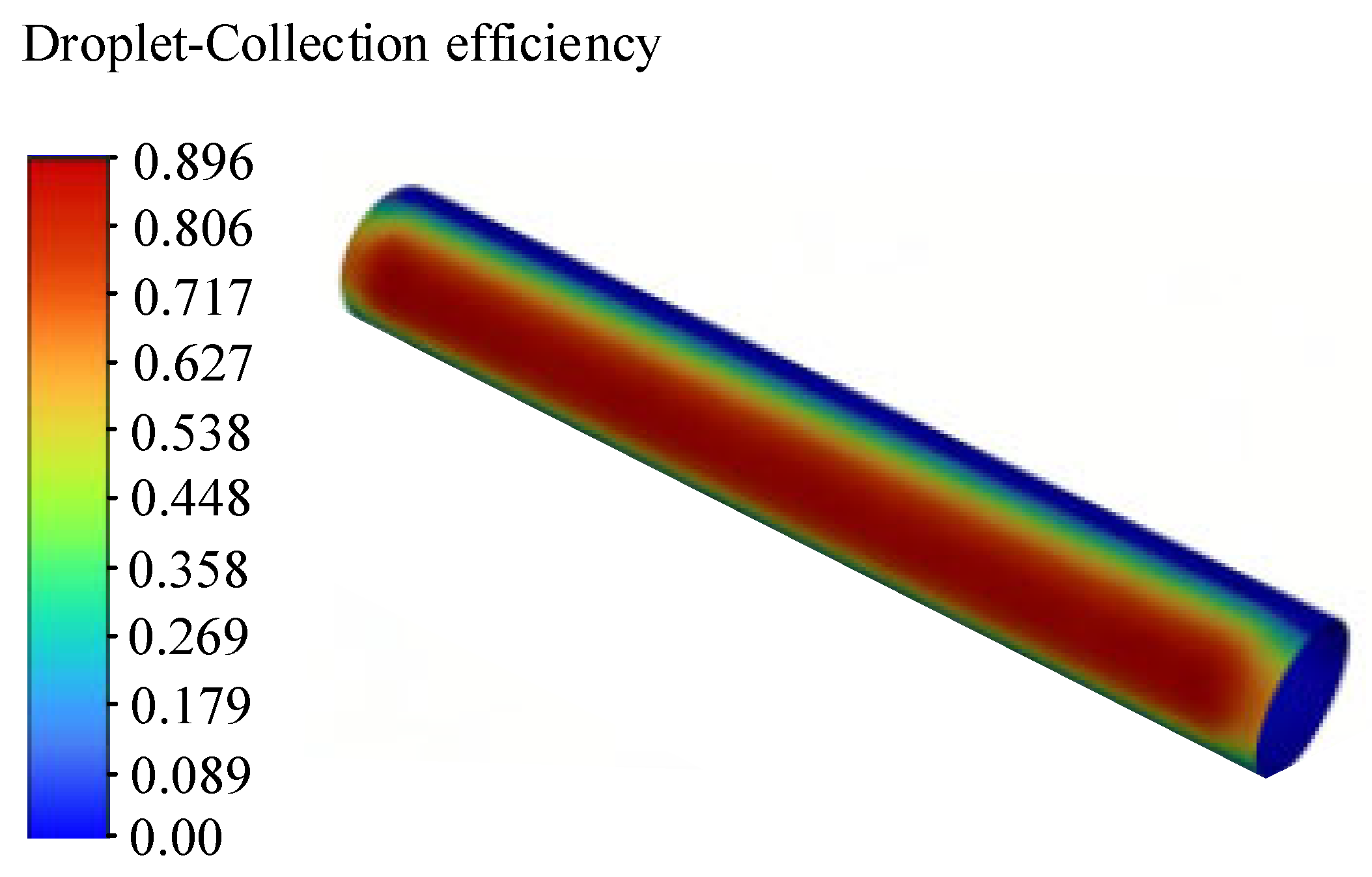
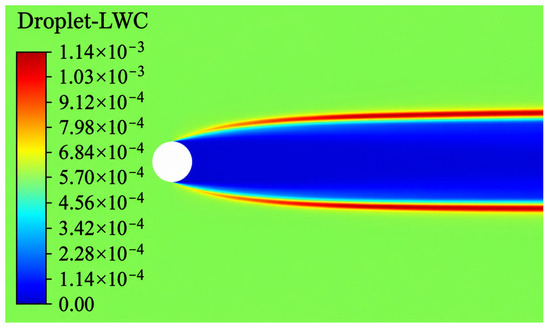
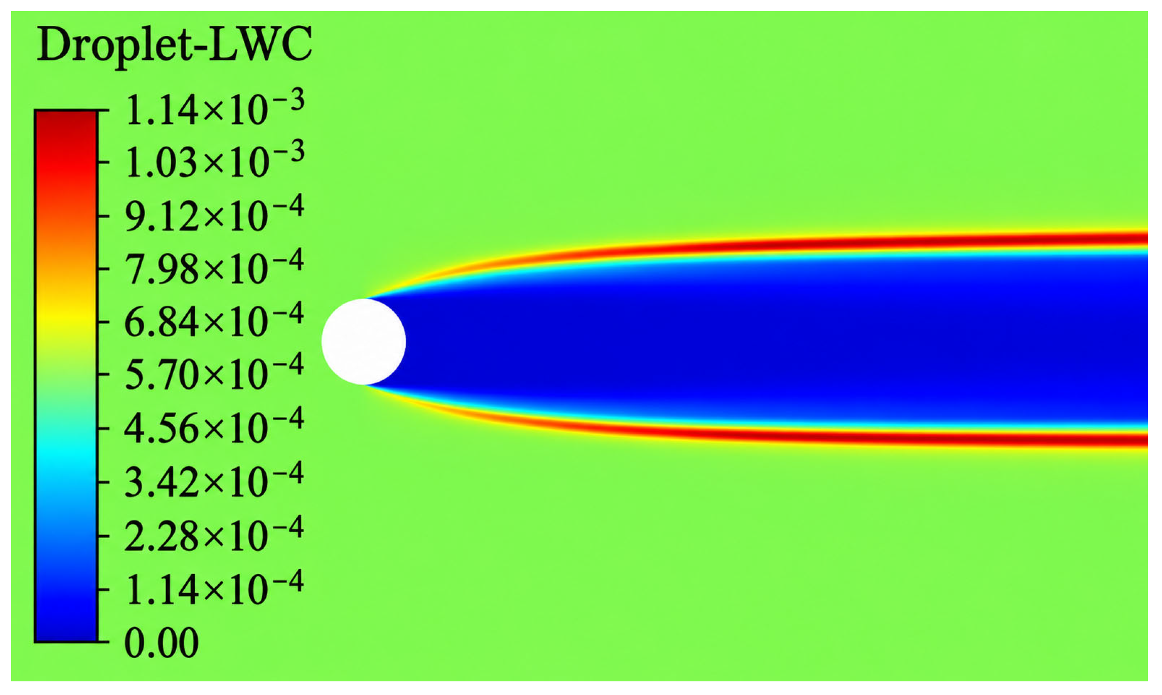
A representative case of the auxiliary conductor was selected for numerical validation. The simulation conditions were specified as an incoming wind speed of 5 m/s, an ambient temperature of −5 °C, a droplet diameter of 25 μm, and a liquid water content of 0.5 g/m³. The analysis was divided into three time intervals, and the results were recorded every 10 min. Figure 5 presents the contour distribution of the droplet collection efficiency on the surface of the auxiliary conductor. Different colors represent the droplet collection efficiency at different locations on the conductor surface, allowing the regions with more pronounced droplet accumulation to be identified visually. Figure 6 shows the distribution of liquid water content (LWC) around the auxiliary conductor, where the blue contour indicates the shadow region in which no droplets are present.

Figure 5. Contour distribution of droplet collection efficiency on the auxiliary conductor surface.

Figure 6. Distribution of liquid water content (LWC).

As shown in Figure 5, because the auxiliary conductor has a regular circular cross-section, the surrounding flow field exhibits a high degree of symmetry. As the airflow approaches the windward surface of the conductor, its velocity gradually decreases owing to the blockage effect of the conductor, forming an approximate stagnation region at the leading edge. Because of their inertia, the supercooled water droplets entrained in the airflow cannot completely follow the streamlines around the conductor and therefore tend to impinge preferentially on the leading edge of the windward surface, where the droplet collection efficiency reaches its maximum. Moving from the leading edge toward both sides of the conductor, the airflow accelerates and is deflected along the circular surface, causing an increasing proportion of droplets to bypass the conductor with the flow. Consequently, the number of droplet impacts decreases, and the droplet collection efficiency exhibits a downward trend. As a result, ice accretion on the auxiliary conductor generally initiates at the leading edge of the windward surface and progressively extends toward both sides and around the circumference as the icing duration increases.

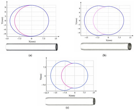
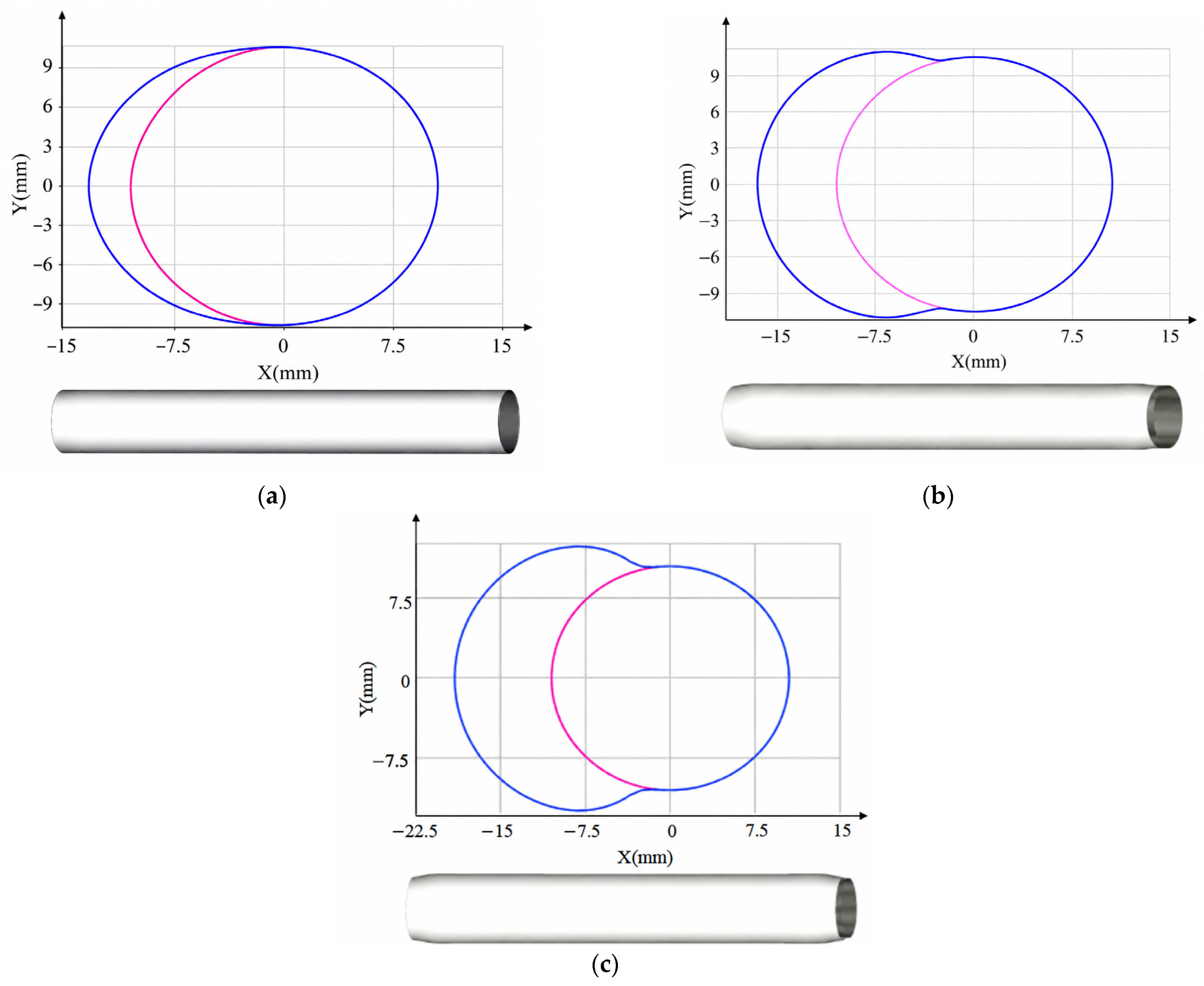
Figure 7 presents the ice shapes of the three-dimensional auxiliary-conductor model at different time steps, illustrating the progressive development of ice accretion during the simulation. Specifically, the pink line represents the original contour of the auxiliary conductor, and the blue line represents the ice accretion profile on the conductor surface.

Figure 7. Ice shapes of the auxiliary conductor at different icing times. (a) Ice shape after 10 min of accretion; (b) ice shape after 20 min of accretion; (c) ice shape after 30 min of accretion.

As shown in Figure 7, under the present wind-speed condition, the inertial effect of the droplets becomes pronounced, and their impact kinetic energy increases approximately with the square of the wind speed, enabling them to strike the conductor surface with greater energy. The increased impact energy not only enhances the droplet collection efficiency and deposition rate on the windward side but also promotes droplet spreading and adhesion on the surface, thereby accelerating the initial growth of the ice layer in the windward region. Meanwhile, as the wind speed increases, the flow around the conductor intensifies, and the streamlines contract and accelerate markedly along its upper and lower sides. Consequently, some droplets that do not directly impinge on the windward surface are deflected by aerodynamic forces, entrained by the main flow, and transported along both sides of the conductor. This process causes the icing region to expand progressively from the windward surface toward the upper and lower sides, producing an ice distribution that extends in the flow direction.

It should be noted that the parametric analysis in this section is primarily intended to reveal the qualitative influence trends of environmental factors on ice accretion on auxiliary conductors, rather than to provide quantitatively calibrated predictions of absolute ice thickness or icing coverage. In actual railway environments, variations in wind direction, conductor torsion, stranded-surface geometry, and other three-dimensional effects may redistribute droplet impingement around the conductor circumference and consequently produce more irregular icing patterns. Therefore, the discussion focuses mainly on the relative variations in ice morphology, ice thickness, and icing extent under different environmental conditions.

2.4.1. Effect of Wind Speed on Ice Accretion on the Auxiliary Conductor

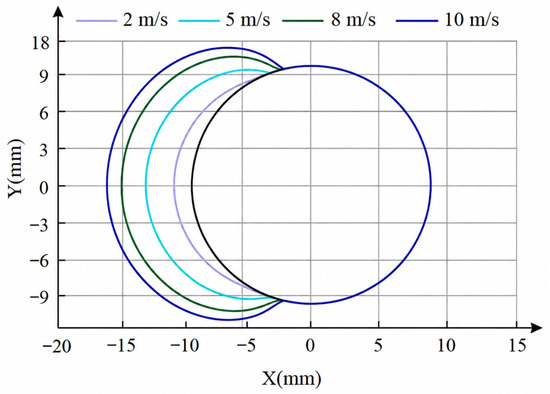
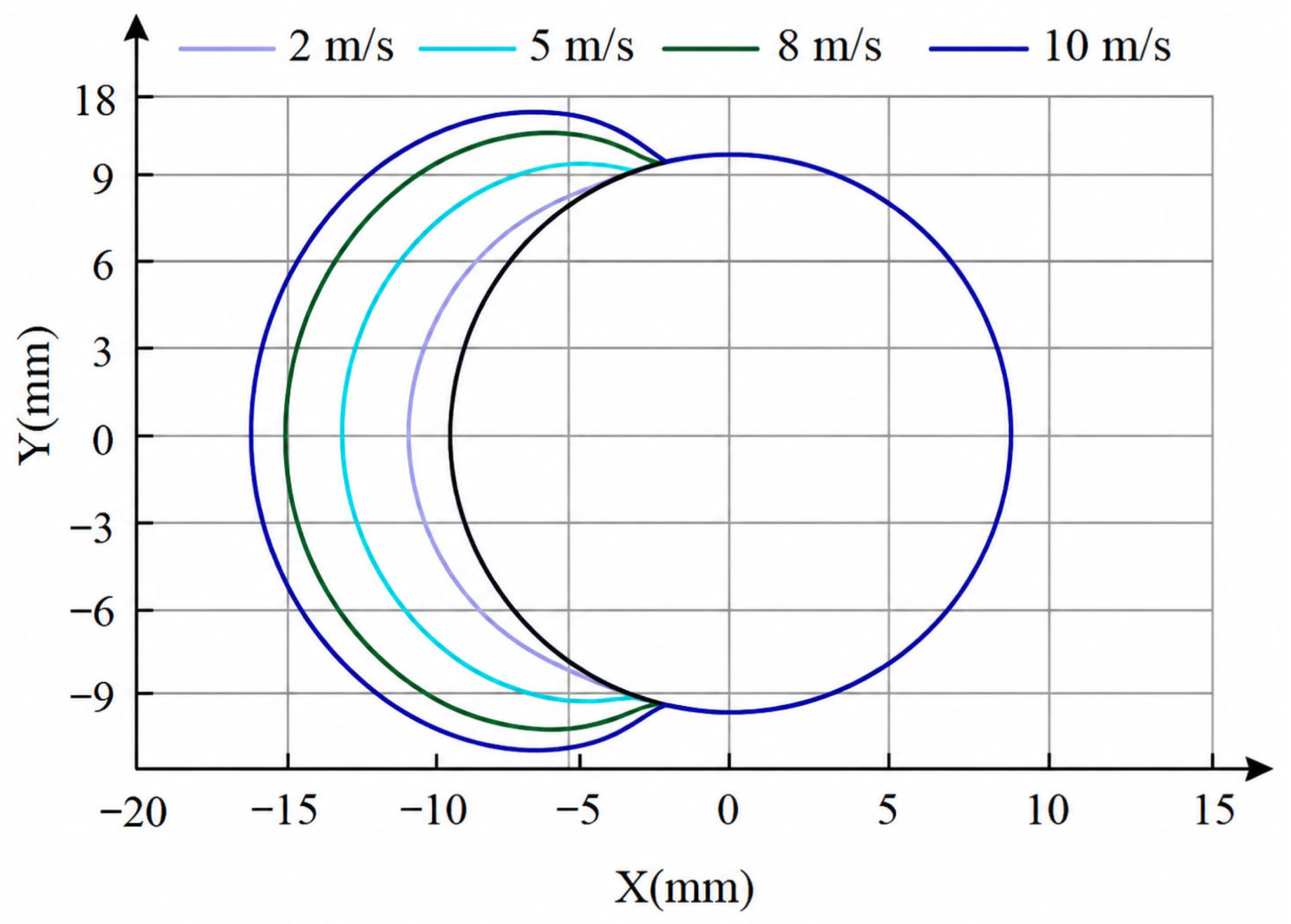
As discussed above, wind speed mainly affects conductor icing through its influence on the droplet collection efficiency. As the wind speed increases, the kinetic energy of the droplets increases, making their trajectories less susceptible to deflection by the airflow and thereby enlarging the droplet impingement region. In this study, the liquid water content, droplet diameter, and ambient temperature were kept constant at 0.5 g/m³, 25 μm, and −5 °C, respectively, while the wind speed was varied as 2, 5, 8, and 10 m/s. The ice shapes of the auxiliary conductor under different wind-speed conditions are shown in Figure 8. Specifically, the black line represents the original contour of the auxiliary conductor without ice accretion, while the colored lines represent the ice accretion profiles under different wind speeds.

Figure 8. Ice shapes of the auxiliary conductor at different wind speeds.

As shown in Figure 8, as the incoming wind speed increases, the ice thickness on the conductor surface increases continuously. Meanwhile, the upper and lower impingement limits extend from the leading-edge stagnation point toward the leeward side, resulting in a progressively wider icing region and, ultimately, a fuller ice-profile contour. This behavior can be attributed to two main mechanisms. First, a higher wind speed increases the velocity and inertial effect of the supercooled water droplets, thereby enhancing the droplet collection efficiency on the conductor surface. Consequently, more droplets collide with and are captured by the conductor per unit time, leading to higher ice-growth rates and a greater maximum ice thickness. Second, at higher wind speeds, the droplets are less able to follow changes in the airflow streamlines and are therefore less strongly deflected as they pass around the conductor. As a result, they can impinge on the conductor surface at locations farther from the leading-edge stagnation point. Accordingly, the droplet impingement limits extend farther along the upper and lower sides of the conductor, shifting the icing limits downstream and enlarging the overall icing region.

2.4.2. Effect of Droplet Diameter on Ice Accretion on the Auxiliary Conductor

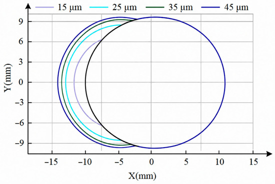
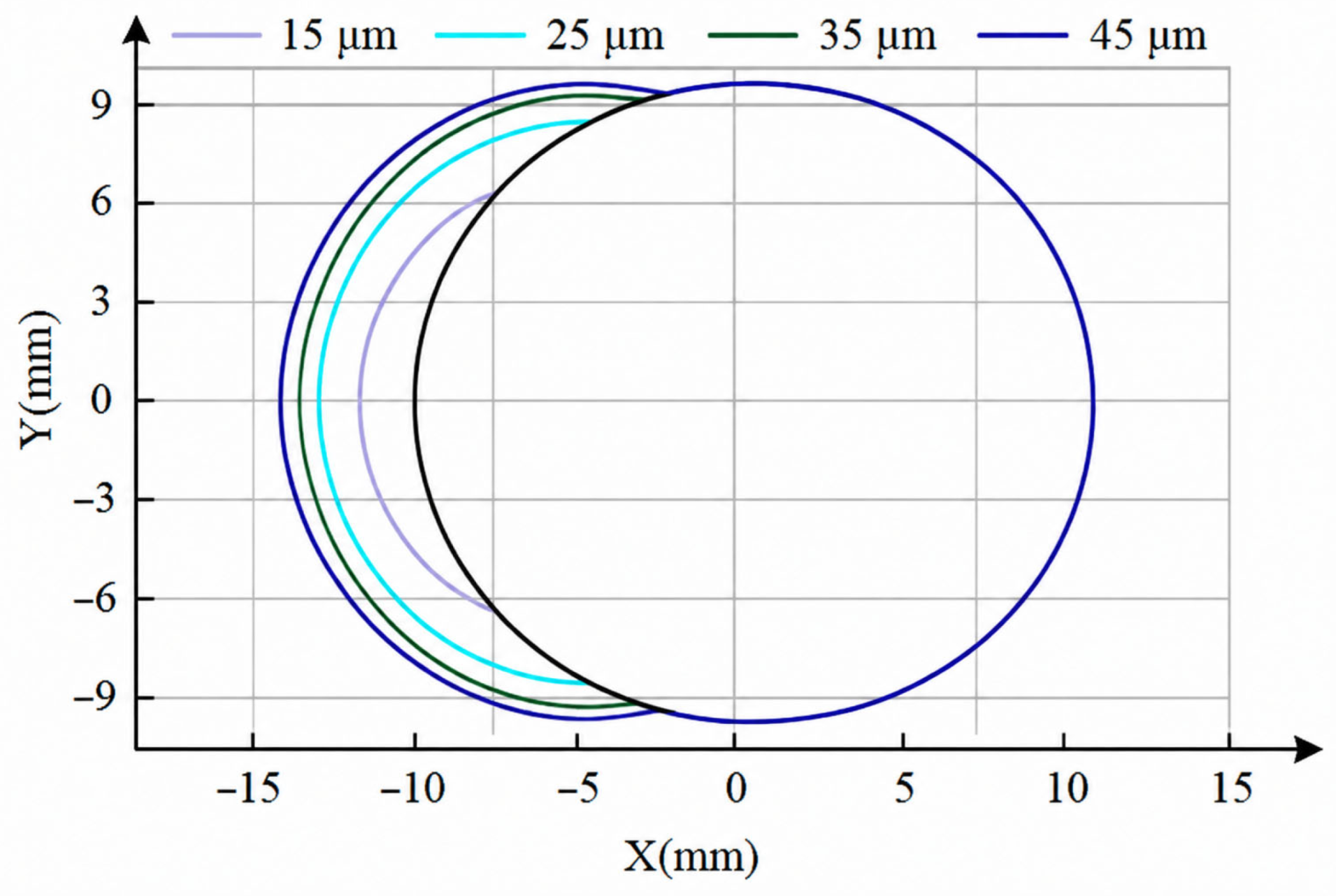
The wind speed, liquid water content, and ambient temperature were maintained at 5 m/s, 0.5 g/m³, and −5 °C, respectively. Under icing conditions, the diameters of atmospheric droplets are generally below 40 μm. Accordingly, the droplet median volume diameter (MVD) was varied in a stepwise manner as 15, 25, 35, and 45 μm. The resulting ice shapes of the auxiliary conductor are shown in Figure 9, enabling the influence of droplet diameter on the conductor ice morphology to be examined. Specifically, the black line represents the original contour of the auxiliary conductor without ice accretion, while the colored lines represent the ice accretion profiles under different wind speeds.

Figure 9. Ice shapes of the auxiliary conductor under different droplet diameters [41].

Figure 9 shows the ice shapes of the auxiliary conductor under different droplet diameters. It can be seen that, as the droplet diameter increases, both droplet mass and inertial effects become stronger, leading to more stable trajectories in the airflow and a reduced sensitivity to turbulent disturbances and viscous forces. As a result, larger droplets are more likely to deviate from the airflow streamlines and directly impinge on the conductor surface, thereby increasing the number of captured droplets and expanding both the droplet collection efficiency and the impingement limit. In contrast, smaller droplets possess weaker inertia and are more easily influenced by the surrounding airflow during their motion. Some of these droplets are carried around the conductor by the flow and therefore cannot effectively strike the conductor surface. Under such conditions, ice accretion is mainly concentrated on the windward side of the conductor, and the resulting ice layer is relatively thin with a limited coverage range. As the droplet diameter gradually increases, more droplets are able to reach and deposit on the auxiliary conductor surface, causing the icing region to expand continuously toward the upper and lower sides of the conductor. Consequently, the ice profile becomes fuller, although the increase in ice thickness is not pronounced.

2.4.3. Effect of Liquid Water Content on Ice Accretion on the Auxiliary Conductor

Liquid water content (LWC) is an important parameter used to characterize the amount of suspended liquid water in the air and mainly reflects the concentration of droplets available for freezing. During the icing process, LWC directly affects the droplet impingement frequency and deposition mass on the surface of the auxiliary conductor and is therefore one of the key factors governing the ice-growth rate and final ice thickness. When the liquid water content is high, the number of suspended droplets in the air increases, and accordingly, the number of droplets impinging on the conductor surface per unit time rises significantly.

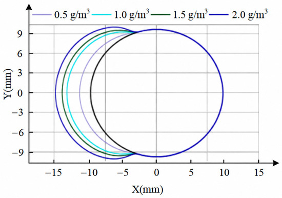
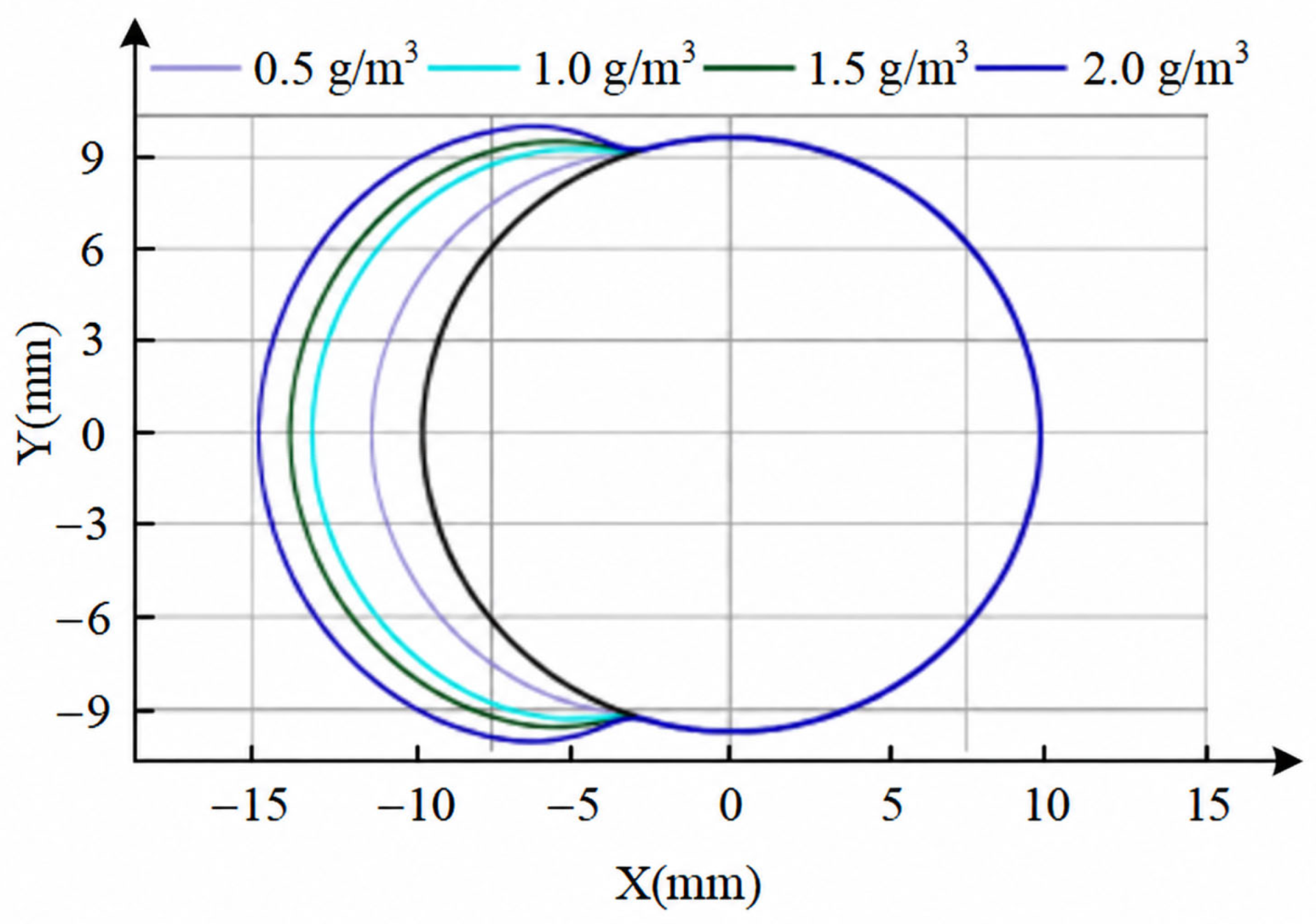
In this study, the wind speed, droplet diameter, and ambient temperature were kept constant at 5 m/s, 25 μm, and −5 °C, respectively, while the liquid water content was varied as 0.5, 1.0, 1.5, and 2.0 g/m³. The resulting ice shapes of the auxiliary conductor under different liquid water content conditions are shown in Figure 10. Specifically, the black line represents the original contour of the auxiliary conductor without ice accretion, while the colored lines represent the ice accretion profiles under different wind speeds.

Figure 10. Ice shapes of the auxiliary conductor under different liquid water content conditions.

As shown in Figure 10, the liquid water content represents the concentration of supercooled droplets in the airflow, namely, the total mass of liquid water contained per unit volume of air. As the liquid water content increases, the number of droplets available for impingement, freezing, and deposition rises markedly. With the other environmental parameters held constant, more droplets are transported toward and impinge on the conductor surface per unit time, thereby increasing the amount of water captured and frozen on the surface. Consequently, the ice-growth rate increases and the ice layer becomes substantially thicker. However, variations in liquid water content primarily affect the number of droplets and do not significantly alter droplet inertia or their impingement locations on the conductor surface. Therefore, although the ice layer thickens continuously with increasing liquid water content, the upper and lower icing limits change only slightly, while the overall icing coverage and ice-shape profile remain essentially unchanged.

2.4.4. Effect of Ambient Temperature on Ice Accretion on the Auxiliary Conductor

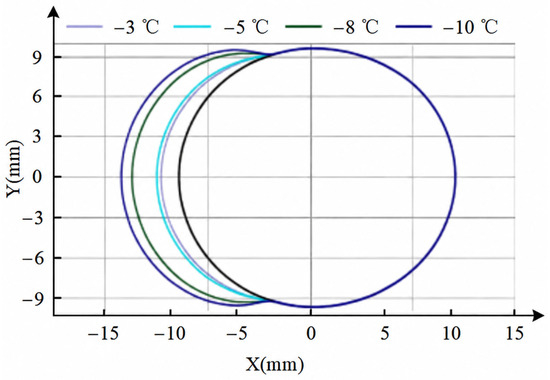
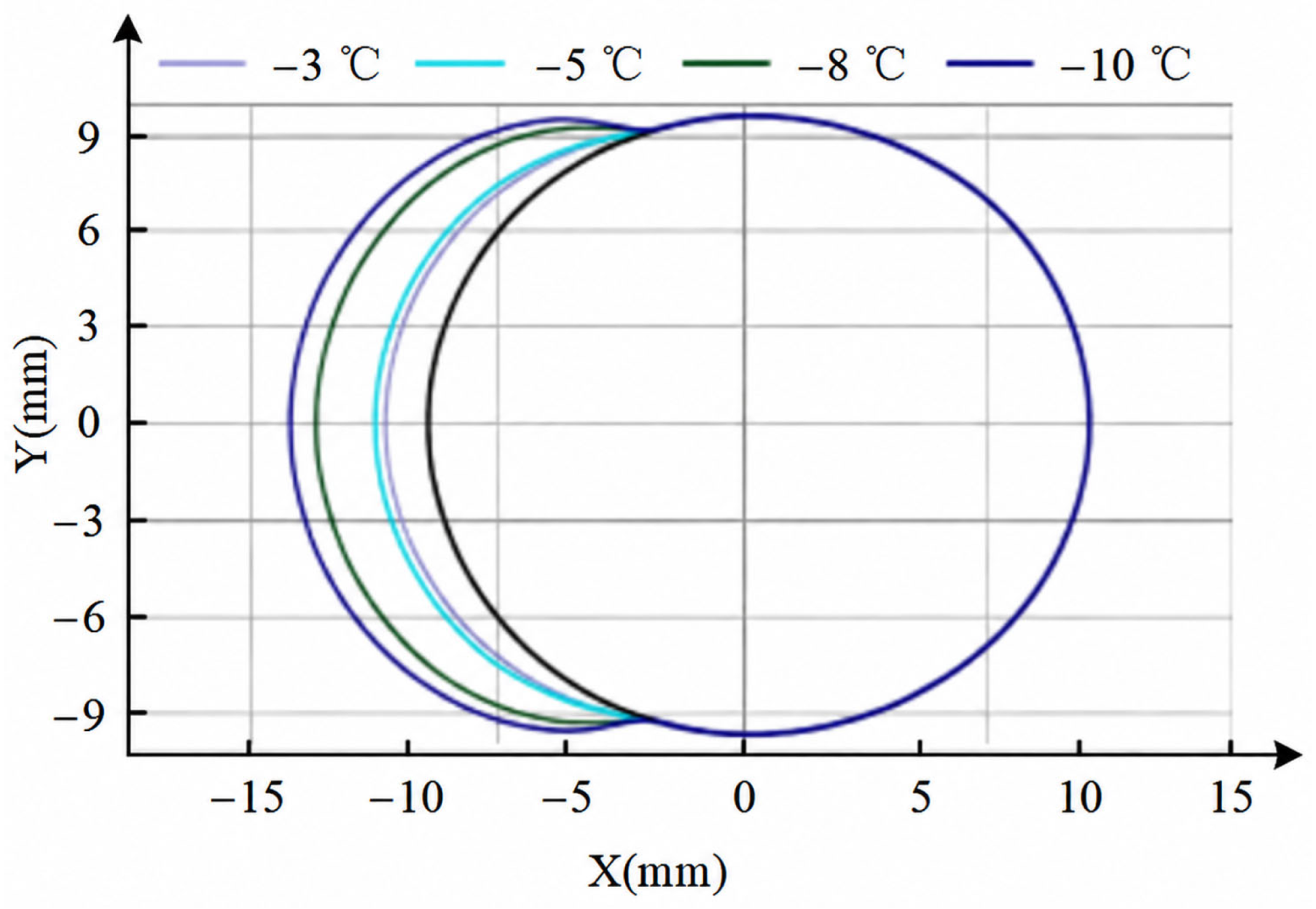
The freezing behavior of water droplets is closely related to the ambient temperature. Variations in temperature alter the droplet-freezing rate and freezing efficiency, thereby significantly affecting both the growth mode of the ice layer and the final ice morphology. To investigate the influence of ambient temperature on the icing process, the wind speed, liquid water content, and droplet diameter were maintained at 5 m/s, 0.5 g/m³, and 25 μm, respectively, while the ambient temperature was varied as −3, −5, −8, and −10 °C. The ice shapes of the auxiliary conductor under different temperature conditions are shown in Figure 11. Specifically, the black line represents the original contour of the auxiliary conductor without ice accretion, while the colored lines represent the ice accretion profiles under different wind speeds.

Figure 11. Ice shapes of the auxiliary conductor under different ambient temperatures.

As shown in Figure 11, within the temperature range from −3 °C to −10 °C, the ice thickness on the windward side of the conductor increases progressively as the ambient temperature decreases, and the outer contour of the ice shape extends more prominently toward the incoming flow. At relatively high temperatures, the droplets undergo a certain degree of spreading and redistribution after impact, resulting in a smoother ice layer with a smaller thickness and a more gradual overall change in contour. When the temperature decreases to −5 °C and −8 °C, the droplet-freezing rate increases, causing the windward-side ice layer to thicken progressively and the ice shape to protrude further upstream. Under the −10 °C condition, the droplets freeze almost instantaneously, and liquid-water migration is greatly suppressed, leading to concentrated ice accumulation on the windward surface and the maximum ice thickness. Because the conductor cross-section is a regular circle and its aerodynamic structure is relatively symmetric, the main effect of temperature is reflected in the difference in windward-side ice thickness, while the overall ice shape still maintains a good degree of axisymmetry.

3. Numerical Analysis of Auxiliary-Conductor Galloping

3.1. Development of the Computational Domain

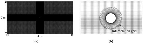
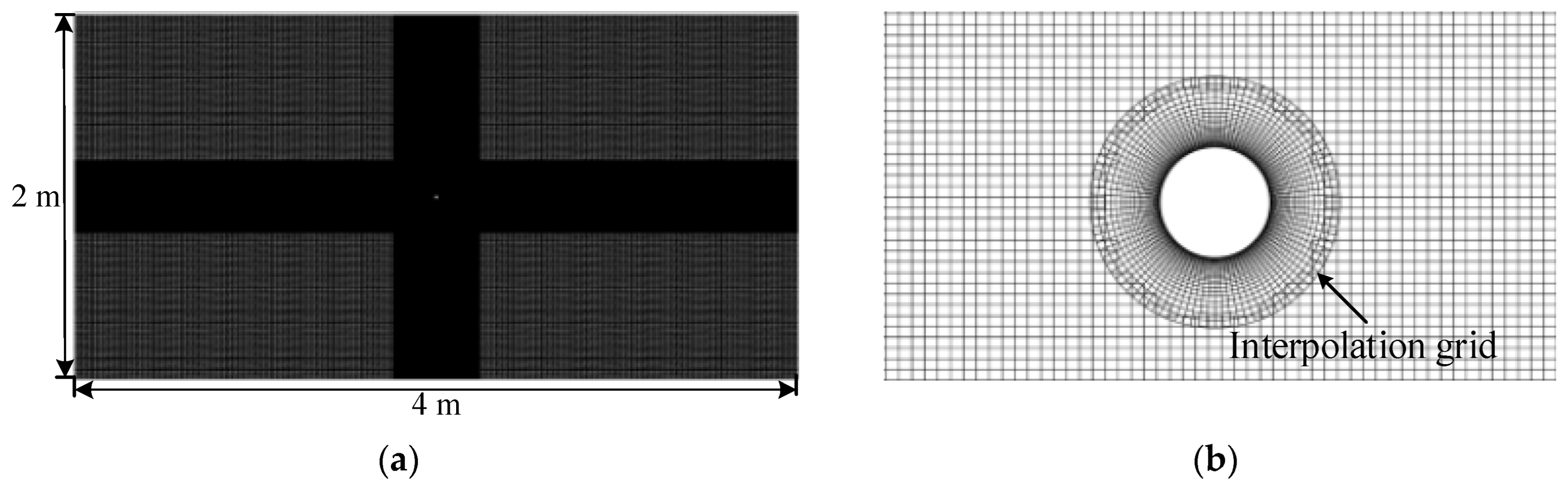
During actual operation of an overhead contact system, auxiliary conductors are continuously exposed to natural wind environments. Once ice accretes on the conductor surface, the cross-section changes from a regular circular shape to an asymmetric profile, resulting in significant changes in the mass per unit length, projected windward area, and aerodynamic characteristics of the conductor. Under sustained wind loading, an iced auxiliary conductor may exhibit large-amplitude, low-frequency coupled horizontal and vertical vibrations; in severe cases, this develops into galloping, which increases the midspan displacement and the dynamic loads at the suspension points, thereby adversely affecting the service safety of the conductor and its associated fittings. Therefore, to reveal the fundamental galloping characteristics of iced auxiliary conductors, a two-dimensional, two-degree-of-freedom numerical model for galloping response was first established. The computational domain was defined as 2 m × 4 m. Because the conductor may undergo relatively large displacements in both the horizontal and vertical directions during galloping, the mesh in the conductor-motion region must be updated continuously. To reduce the computational errors caused by mesh distortion induced by conductor motion, an overset-mesh technique was adopted to represent the moving conductor boundary within the flow field. The overset mesh consisted of two parts: a stationary background mesh and a component mesh. The stationary mesh did not move with the conductor and therefore did not deform due to stretching or compression. Both the background mesh and the component mesh were structured meshes, and the dimensionless wall distance of the boundary-layer mesh near the conductor surface was kept below 1. The computational domain and mesh configuration are shown in Figure 12.

Figure 12. Computational mesh of the flow field around the auxiliary conductor. (a) Overall flow-field mesh; (b) interpolation mesh.

3.2. Fluid–Structure Interaction Computational Method

Fluid–structure interaction (FSI) refers to a multiphysics coupling problem arising from the interaction between a fluid field and a structural field through their common interface. In such problems, aerodynamic loads generated by the fluid, including pressure and viscous shear stress, act on the structural surface and induce deformation, vibration, or rigid-body motion. Meanwhile, structural displacement and deformation alter the boundary geometry and constraints of the fluid domain, thereby redistributing the flow field and producing a characteristic two-way feedback mechanism. This process reflects the strong coupling between fluid dynamics and structural dynamics.

According to the coupling strategy, FSI can be classified into one-way and two-way coupling. One-way coupling considers only the fluid loads acting on the structure while neglecting the feedback of the structural response on the flow field. It is generally applicable to structures with high stiffness or small deformation. In contrast, two-way coupling accounts for the mutual feedback between the fluid and structure, whereby structural motion modifies the fluid boundary conditions in real time and consequently affects the evolution of the flow field. Although two-way FSI is considerably more complex to implement numerically than one-way coupling, it is essential for problems involving strong aerodynamic excitation. In the simulation of auxiliary-conductor galloping, the conductor vibrates under incoming wind loads, while its motion simultaneously alters the local airflow distribution and aerodynamic forces. Therefore, auxiliary-conductor galloping represents a typical two-way FSI problem.

In FSI analysis, the Newmark-β method is widely used to solve the dynamic response of structures. Its basic principle is to determine the structural displacement, velocity, and acceleration through time-stepping integration while accounting for the influence of fluid loads. The governing equation of structural dynamics is expressed as follows:

$$M\ddot{u}(t)+C\dot{u}(t)+Ku(t)=F(t),$$

(15)

where $M$ is the structural mass matrix, $C$ is the structural damping matrix, $K$ is the structural stiffness matrix, $u(t)$ is the conductor displacement vector, $\dot{u}(t)$ is the conductor velocity vector, $\ddot{u}(t)$ is the conductor acceleration vector, and $F(t)$ is the external force exerted by the fluid.

In the Newmark-β method, Equation (15) is discretized to perform time integration. The iterative expressions for displacement and velocity are given as follows:

$$x_{n+1}=x_n+\Delta t{\dot{x}}_n+\left({\displaystyle \frac{1}{2}}-\beta \right)\Delta t^2{\ddot{x}}_n+\beta \Delta t^2{\ddot{x}}_{n+1},$$

(16)

$${\dot{x}}_{n+1}={\dot{x}}_n+(1-\gamma )\Delta t{\ddot{x}}_n+\gamma \Delta t{\ddot{x}}_{n+1},$$

(17)

where $x_n$ and $x_{n+1}$ denote the displacements at time steps n and n + 1, respectively, ${\dot{x}}_n$ and ${\dot{x}}_{n+1}$ denote the velocities at time steps n and n + 1, respectively, and ${\ddot{x}}_n$ and ${\ddot{x}}_{n+1}$ denote the accelerations at time steps n and n + 1, respectively. $\Delta t$ is the time-step size, while β and γ are parameters of the Newmark method that control the time-integration accuracy of acceleration and velocity, respectively. In general, β = 1/4 and γ = 1/2 are adopted to ensure numerical stability.

In fluid–structure interaction analysis, the aerodynamic loads exerted by the fluid on the structure are generally determined through fluid-flow simulations. The following coupling algorithm is commonly employed to calculate the fluid loads by relating the fluid velocity and pressure to the structural displacement and velocity:

$$F_{fluid}(t)={\displaystyle {\int }_0^t\left({\rho }_{fluid}\cdot A_{fluid}\cdot {\overrightarrow{v}}_{fluid}(t)\right)}dt,$$

(18)

where ${\rho }_{fluid}$ is the fluid density, $A_{fluid}$ is the area subjected to fluid loading, and ${\overrightarrow{v}}_{fluid}(t)$ is the fluid velocity field. The aerodynamic load $F_{fluid}(t)$ is dynamically updated according to the deformation state of the overhead contact system, thereby influencing the structural vibration response.

The numerical solution of fluid–structure interaction problems generally requires dynamic tracking of structural displacement, velocity, and acceleration while simultaneously accounting for the forces exerted by the fluid on the structure. Within the framework of the Newmark-β method, the time-stepping scheme incorporates both the structural dynamic behavior and the temporal variation in the fluid loads. By iteratively exchanging the structural deformation and fluid-response data, a stable numerical solution can ultimately be obtained.

A conductor subjected to wind loading and other external excitations may undergo vibration, whose dynamic behavior can be described using either a lumped-mass model or a continuum model. Based on force equilibrium, the vibration of the conductor can be governed by the following partial differential equation:

$$m{\displaystyle \frac{{\mathsf{\partial }}^{2}u(x,t)}{\mathsf{\partial }{t}^2}}+c{\displaystyle \frac{\mathsf{\partial }u(x,t)}{\mathsf{\partial }t}}+ku(x,t)=F(x,t),$$

(19)

where $m{\displaystyle \frac{{\mathsf{\partial }}^{2}u(x,t)}{\mathsf{\partial }{t}^2}}$ is the mass term representing the inertia of the conductor, $c{\displaystyle \frac{\mathsf{\partial }u(x,t)}{\mathsf{\partial }t}}$ is the damping term describing the energy dissipated during vibration, $ku(x,t)$ is the restoring-force term representing the elastic behavior of the conductor, and $F(x,t)$ is the external load.

In a fluid–structure interaction problem, the conductor is subjected not only to external wind loading but also to aerodynamic forces generated by the surrounding flow. These aerodynamic forces modify the conductor vibration modes and consequently affect its dynamic stability. Therefore, the feedback effect of the aerodynamic loads must be incorporated into the governing equation of conductor motion. The aerodynamic load $F_{aero}(x,t)$ acting on the conductor can be expressed as follows:

$$F_{aero}(x,t)=C_D\cdot {\displaystyle \frac{1}{2}}{\rho }_a{U}^2(x,t)A(x),$$

(20)

where $C_D$ is the conductor drag coefficient, ${\rho }_a$ is the air density, $U(x,t)$ is the relative wind speed at position x and time t on the conductor surface, and $A(x)$ is the conductor cross-sectional area at position x.

Therefore, the governing dynamic equation of the conductor under fluid–structure interaction can be expressed as follows:

$$m{\displaystyle \frac{{\mathsf{\partial }}^{2}u(x,t)}{\mathsf{\partial }{t}^2}}+c{\displaystyle \frac{\mathsf{\partial }u(x,t)}{\mathsf{\partial }t}}+ku(x,t)=F(x,t)+F_{aero}(x,t),$$

(21)

where $F(x,t)$ includes all external loads other than aerodynamic forces, such as gravity and ice loads, whereas $F_{aero}(x,t)$ denotes the aerodynamic force exerted by the fluid on the conductor.

To simplify the computation, the conductor equation of motion is approximated using a two-degree-of-freedom model in the numerical simulation of the vibration response, where $u(t)=\left(\begin{array}{l}x(t)\\ y(t)\end{array}\right)$. The corresponding simplified single-degree-of-freedom equation of motion is given in Equation (22), in which $F_{aero}(t)$ denotes the external force.

$$M\ddot{u}(t)+C\dot{u}(t)+Ku(t)=F(t)+F_{aero}(t),$$

(22)

In the vibration-response simulation, the conductor is treated as a rigid body, and only its cross-flow vibration induced by the lift generated by the Kármán vortex street is considered. The vibration response is described using a fluid–structure interaction mechanical model. By neglecting conductor deformation, the governing equation of motion can be expressed as follows:

$$\left\{\begin{array}{l}m\ddot{x}+c\dot{x}+kx={\displaystyle \frac{1}{2}}{C}_D{\rho }_a{AU}^2\\ m\ddot{y}+c\dot{y}+ky={\displaystyle \frac{1}{2}}{C}_L{\rho }_a{AU}^2\end{array}\right.,$$

(23)

where x and y are the horizontal and vertical displacement responses of the conductor, respectively; m is the conductor mass; k is the vertical stiffness; and c is the damping coefficient.

The fourth-order Runge–Kutta method is employed to numerically solve the transverse vibration response $x(t)$ of the conductor. By expressing the conductor vibration displacement and velocity as the state vector $Y(t)$, the equation of motion can be transformed into the following system of ordinary differential equations:

$$\dot{Y}(t)=\left(\begin{array}{l}\dot{x}(t)\\ \dot{y}(t)\\ \ddot{x}(t)\\ \ddot{y}(t)\end{array}\right)=\left(\begin{array}{c}\dot{x}(t)\\ \dot{y}(t)\\ {\displaystyle \frac{1}{m_x}}(F_x-c_x\dot{x}-k_{x}x)\\ {\displaystyle \frac{1}{m_y}}(F_y-c_y\dot{y}-k_{y}y)\end{array}\right),$$

(24)

Using the fourth-order Runge–Kutta method, the state vector $Y(t_{n+1})$ of the conductor at the next time step is obtained as follows:

$$Y(t_{n+1})=Y(t_n)+{\displaystyle \frac{1}{6}}(k_1+2k_2+2k_3+k_4),$$

(25)

where

$$k_1=\Delta t\cdot f(t_n,Y(t_n)),$$

(26)

$$k_2=\Delta t\cdot f\left(t_n+{\displaystyle \frac{\Delta t}{2}},Y(t_n)+{\displaystyle \frac{\Delta t}{2}}{k}_1\right),$$

(27)

$$k_3=\Delta t\cdot f\left(t_n+{\displaystyle \frac{\Delta t}{2}},Y(t_n)+{\displaystyle \frac{\Delta t}{2}}{k}_2\right),$$

(28)

$$k_4=\Delta t\cdot f\left(t_n+\Delta t,Y(t_n)+\Delta t{k}_3\right),$$

(29)

where $k_1$, $k_2$, $k_3$, and $k_4$ are the intermediate variables of the fourth-order Runge–Kutta scheme; $\Delta t$ is the time-step size used in the numerical computation; and $f(t,Y)$ is the function describing the system dynamics in the fourth-order Runge–Kutta method, which is determined by the conductor equation of motion and the aerodynamic loads.

Based on the above method, the conductor displacement under different environmental conditions can be calculated.

3.3. Analysis of Auxiliary-Conductor Galloping Simulation Results

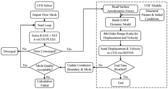
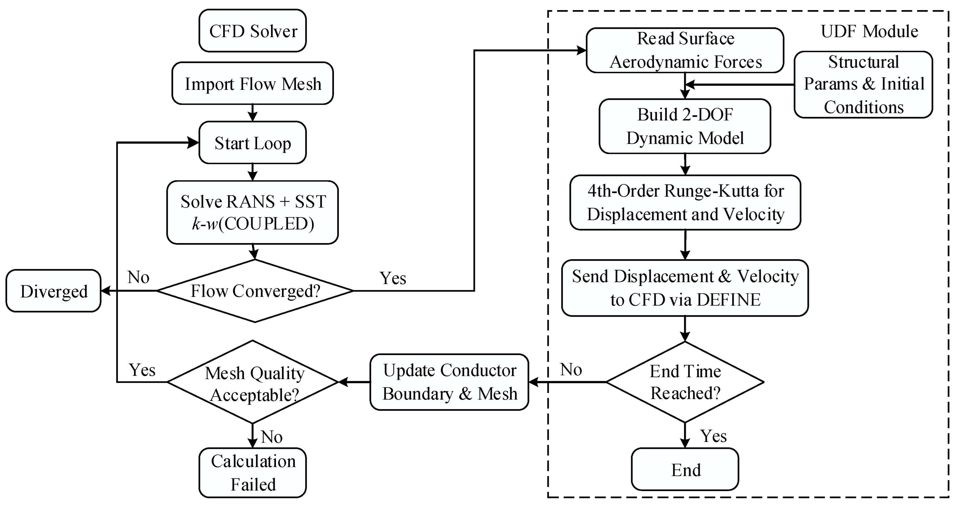
The galloping response of the auxiliary conductor was implemented in Fluent using user-defined functions (UDFs). The procedure was as follows. First, the mesh model was imported and the corresponding boundary conditions were specified. The governing equations were then solved using the COUPLED algorithm, together with the SST k–ω turbulence model to improve the prediction accuracy for flow separation and flow around the conductor. Subsequently, the UDF program was invoked, and the structural equation of motion of the auxiliary conductor was embedded into the CFD solver using DEFINE macros. At each coupling time step, the instantaneous pressure and viscous forces acting on the conductor surface were first obtained from the CFD solution and extracted by the UDF. These aerodynamic forces were then transferred to the two-degree-of-freedom structural model, and the fourth-order Runge–Kutta method was used to calculate the updated horizontal and vertical displacements and velocities. The calculated displacement and velocity were subsequently returned to the CFD solver through the UDF to update the conductor boundary and the overset mesh. The flow field was then recalculated based on the updated conductor position, forming a closed two-way fluid–structure interaction loop. This procedure was repeated until the prescribed simulation time was reached. The flowchart for calculating the galloping response of the auxiliary conductor is shown in Figure 13.

Figure 13. Flowchart of the galloping response analysis for the auxiliary conductor.

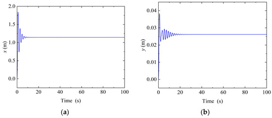
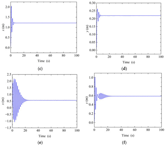
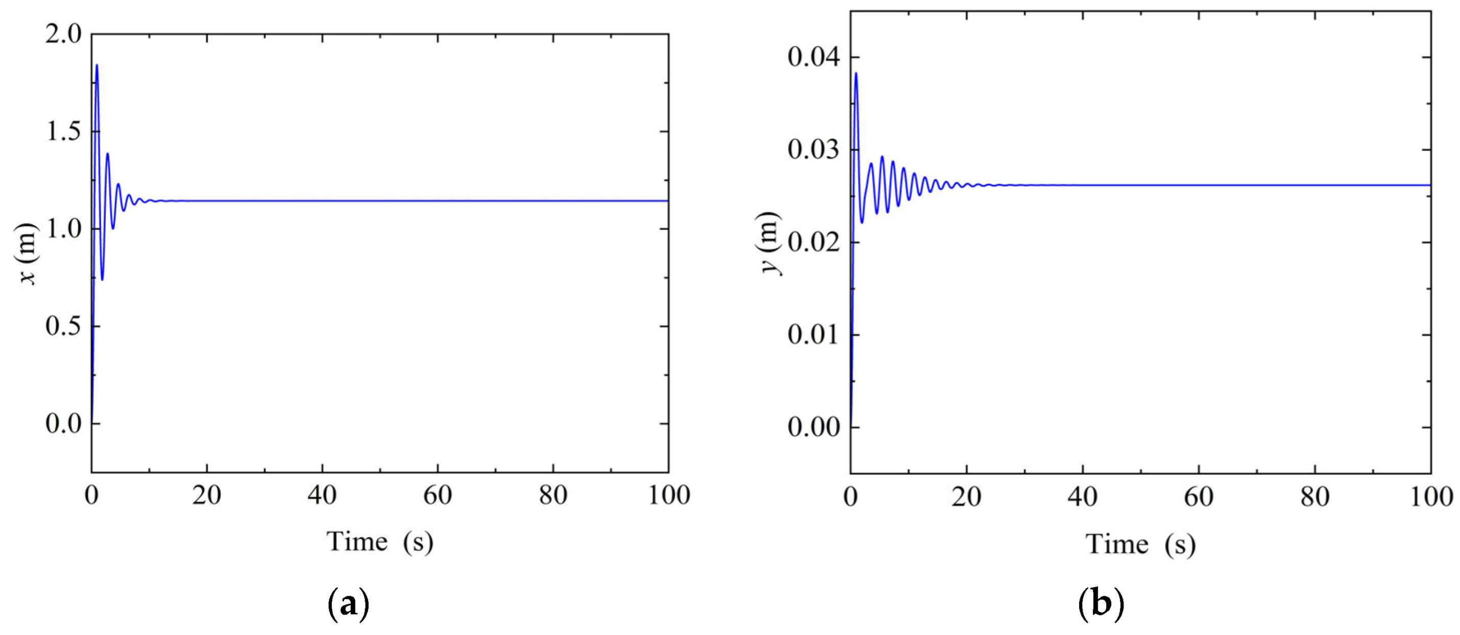
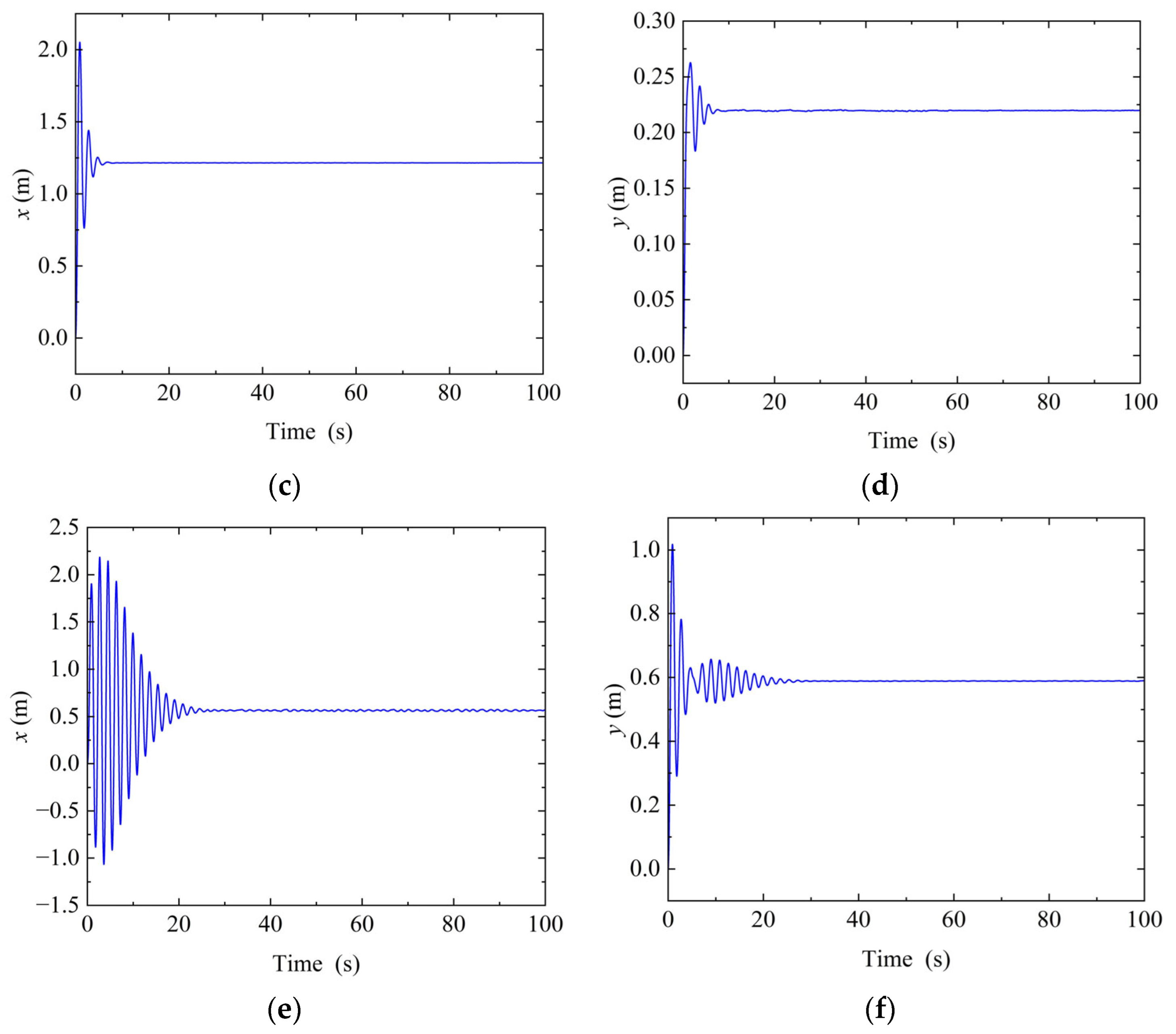
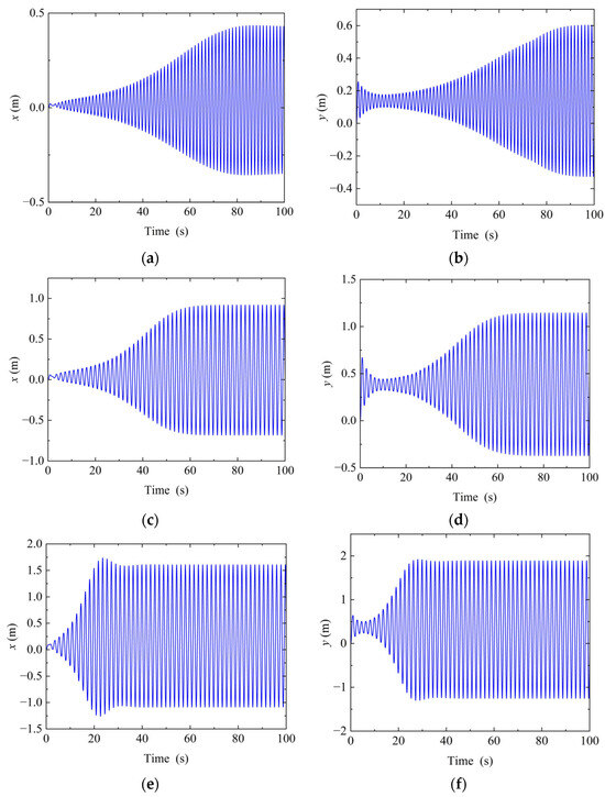
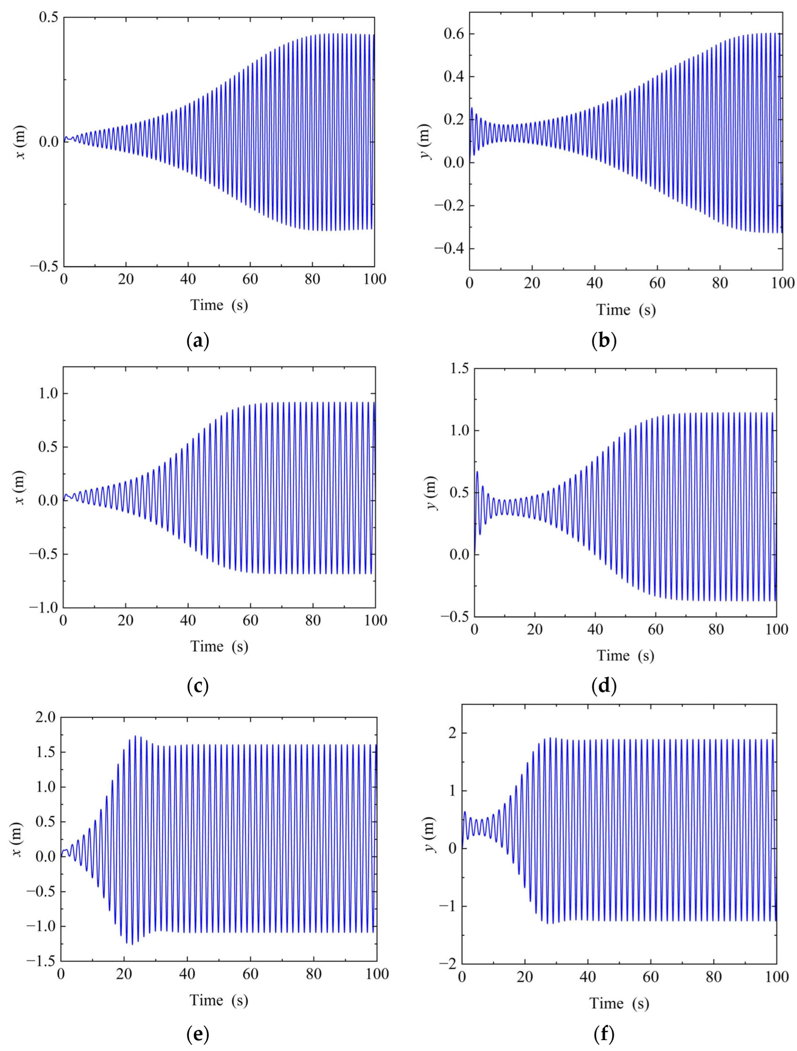
In the structural dynamics model, the mass per unit length of the auxiliary conductor was taken as 1.058 kg/m, the natural frequency was set to 1 Hz, and the damping ratio was specified as 0.002. The crosswind-induced motion of the conductor was described by a second-order ordinary differential equation, in which the combined effects of aerodynamic force and damping force were considered. To ensure the stability and accuracy of the numerical solution, the fourth-order Runge–Kutta method was employed to perform time integration of the structural dynamic equation, thereby obtaining the transient galloping responses of the conductor under different wind-speed conditions. After post-processing the numerical results, time-history curves of the horizontal and vertical displacements of the auxiliary conductor were plotted to analyze the variation characteristics of the galloping response of the iced conductor under different conditions. Two cases were considered, namely, the bare conductor and a conductor with 10 mm crescent-shaped ice, both at an angle of attack of 25°. The corresponding results are shown in Figure 14 and Figure 15.

Figure 14. Displacement time histories of the bare conductor at different wind speeds. (a) v = 10 m/s, horizontal displacement; (b) v = 10 m/s, vertical displacement; (c) v = 15 m/s, horizontal displacement; (d) v = 15 m/s, vertical displacement; (e) v = 20 m/s, horizontal displacement; (f) v = 20 m/s, vertical displacement.

Figure 15. Displacement time histories of the conductor with 10 mm ice accretion at different wind speeds. (a) v = 10 m/s, horizontal displacement; (b) v = 10 m/s, vertical displacement; (c) v = 15 m/s, horizontal displacement; (d) v = 15 m/s, vertical displacement; (e) v = 20 m/s, horizontal displacement; (f) v = 20 m/s, vertical displacement.

Figure 14 presents the horizontal and vertical displacement time histories of the bare auxiliary conductor at different wind speeds. At wind speeds of 10, 15, and 20 m/s, the conductor exhibits transient oscillations of finite amplitude during the initial stage of the simulation. The vibration amplitude then gradually decays, and the conductor eventually stabilizes near the corresponding static equilibrium position. As the wind speed increases, the mean displacement of the conductor changes accordingly, particularly in the vertical direction, where the equilibrium displacement increases from approximately 0.03 m to approximately 0.60 m. However, none of the cases exhibits continuously increasing oscillation amplitudes or sustained large-amplitude periodic motion. This indicates that the aerodynamic characteristics of the bare circular conductor remain relatively symmetric. Following an initial disturbance, structural damping gradually dissipates the vibration energy, and the system remains dynamically stable.

Compared with the bare-conductor cases, the response of the conductor with 10 mm crescent-shaped ice accretion changes markedly. As shown in Figure 15, the crescent-iced conductor exhibits pronounced periodic galloping at all investigated wind speeds, and the response amplitude increases substantially with wind speed. At 10 m/s, the conductor undergoes a short transient adjustment before gradually entering a stable oscillatory state. The horizontal vibration amplitude is relatively small, whereas the vertical vibration is more pronounced, indicating that the galloping response is dominated by vertical motion under this condition. When the wind speed increases to 15 m/s, the amplitudes of both the horizontal and vertical displacements gradually increase with time and approach stable values after approximately 60–70 s. The vibration amplitudes in the two directions become comparable, suggesting that the response evolves from vertically dominated vibration into pronounced coupled horizontal–vertical galloping. When the wind speed is further increased to 20 m/s, the vibration amplitude grows rapidly and develops into stable large-amplitude periodic motion within a relatively short period. The peak displacements in both directions are substantially greater than those observed at the two lower wind speeds, although the vertical vibration remains slightly stronger than the horizontal vibration. Overall, as the wind speed increases from 10 to 20 m/s, the galloping amplitude of the iced conductor increases continuously, the vibration develops more rapidly, and the coupling between the horizontal and vertical motions becomes increasingly pronounced.

A comprehensive comparison demonstrates that the ice shape is a key factor governing the onset of auxiliary-conductor galloping. Under all investigated wind speeds, the bare conductor exhibits only transient vibrations that decay gradually with time. In contrast, ice accretion disrupts the aerodynamic symmetry of the circular cross-section, causing the lift and drag forces to vary nonlinearly with conductor motion and thereby providing sustained aerodynamic energy input to the system. Physically, galloping develops when the aerodynamic work supplied to the moving conductor over an oscillation cycle exceeds the energy dissipated by structural damping. Under this condition, the aerodynamic force effectively reinforces the conductor motion, causing the oscillation amplitude to grow until a stable large-amplitude limit-cycle response is established. As the wind speed increases from 10 to 20 m/s, the galloping response of the iced conductor evolves from small-amplitude periodic vibration dominated by vertical motion into large-amplitude, stable, coupled horizontal–vertical oscillation, with a pronounced increase in galloping amplitude.

3.4. Wind-Tunnel Test Validation

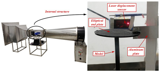
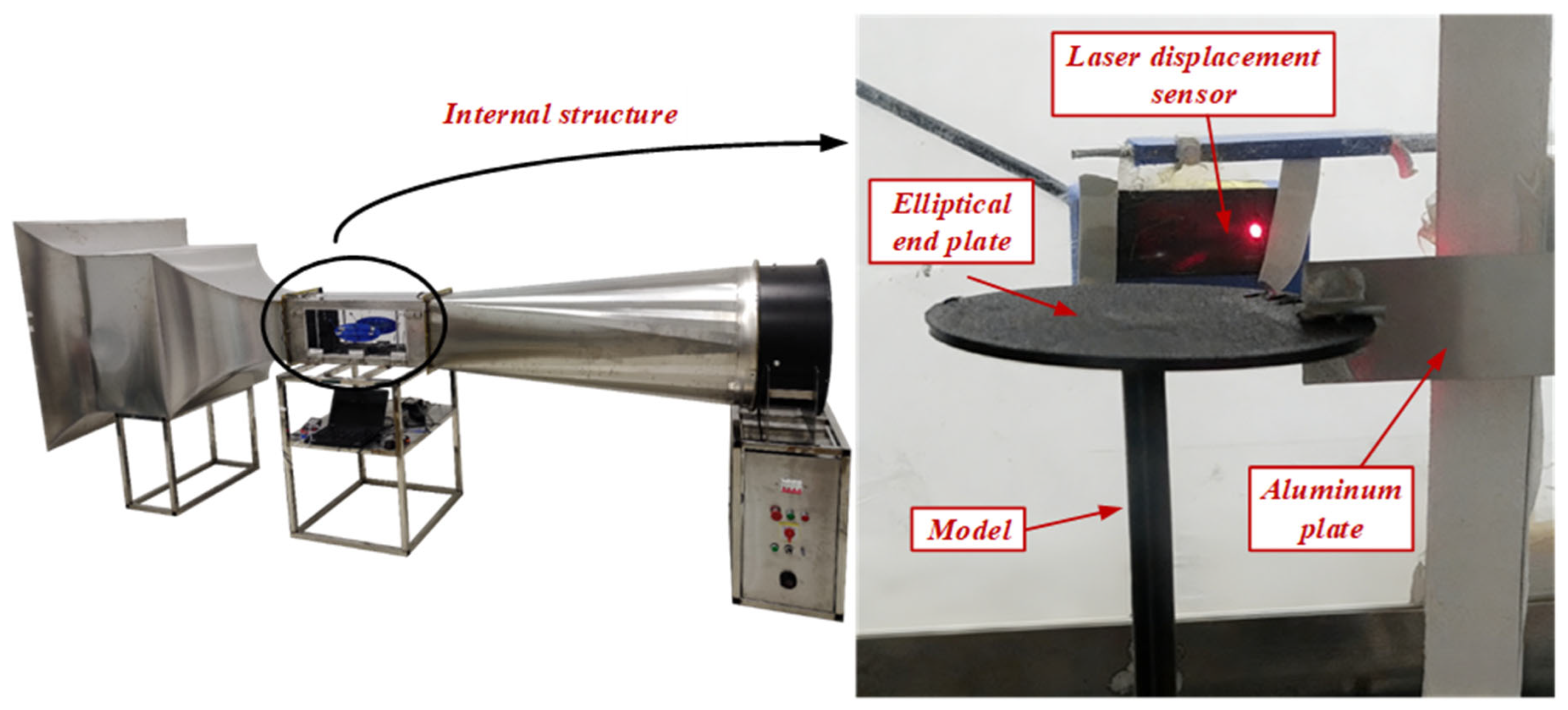
To validate the accuracy and reliability of the CFD simulations, low-speed closed-circuit wind-tunnel tests were conducted. The dimensions of the wind tunnel, the experimental apparatus, and the model installation are shown in Figure 16. The wind-tunnel tests were designed to assess the post-icing aeroelastic response of the auxiliary conductor rather than the ice-accretion process itself, because direct validation of ice growth requires a dedicated icing facility with independently controlled atmospheric icing parameters. The wind tunnel had a total length of 4 m, with a test-section length of 850 mm and a cross-sectional area of 350 mm × 350 mm. The available wind-speed range was 0–20 m/s. Under empty-tunnel conditions, both the incoming-flow turbulence intensity and flow-field nonuniformity were below 0.8%, satisfying the flow-quality requirements for wind-induced vibration tests of iced conductors.

Figure 16. Wind-tunnel test apparatus.

Considering the dimensions of the wind-tunnel test section and the need to maintain sufficient clearance between the vibrating model and the tunnel boundaries, a 1:4-scale iced positive-feeder sectional model was adopted and installed in the test section using aluminum strips and specially designed fixtures. The aluminum strips provided the restoring stiffness required for the sectional vibration system, and their effective lengths were adjusted to achieve the target natural frequency of the experimental model. In this way, the support system reproduced the principal horizontal and vertical elastic characteristics required for the galloping tests without introducing the geometric complexity of a full-span conductor model. An elliptical end plate was installed at one end of the model, and angle-of-attack graduations were fabricated using three-dimensional printing. During the tests, the angle of attack was accurately adjusted by aligning the model with the corresponding graduation. The vibration displacement of the model was measured noncontactly using a Panasonic HG-C1200 laser displacement sensor (Panasonic Industry Co., Ltd., Kadoma, Japan) with a measurement range of ±80 mm. The sensor was used to record displacement time histories under different wind speeds and angles of attack.

The wind-tunnel tests involved six sectional models, each of which was tested at 11 angles of attack: −25°, −20°, −15°, −10°, −5°, 0°, 5°, 10°, 15°, 20°, and 25°, yielding a total of 66 test cases. For each icing angle, the wind speed was increased stepwise. At each wind-speed level, the incoming flow was first allowed to stabilize, and the vibration response of the model was then monitored until a statistically steady state was reached. The displacement time history was subsequently recorded continuously for more than 30 s. The recorded signals were processed to obtain the dimensionless variance and dimensionless vibration amplitude, which were used to characterize the onset and intensity of galloping.

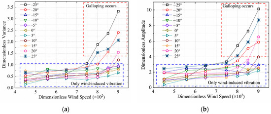
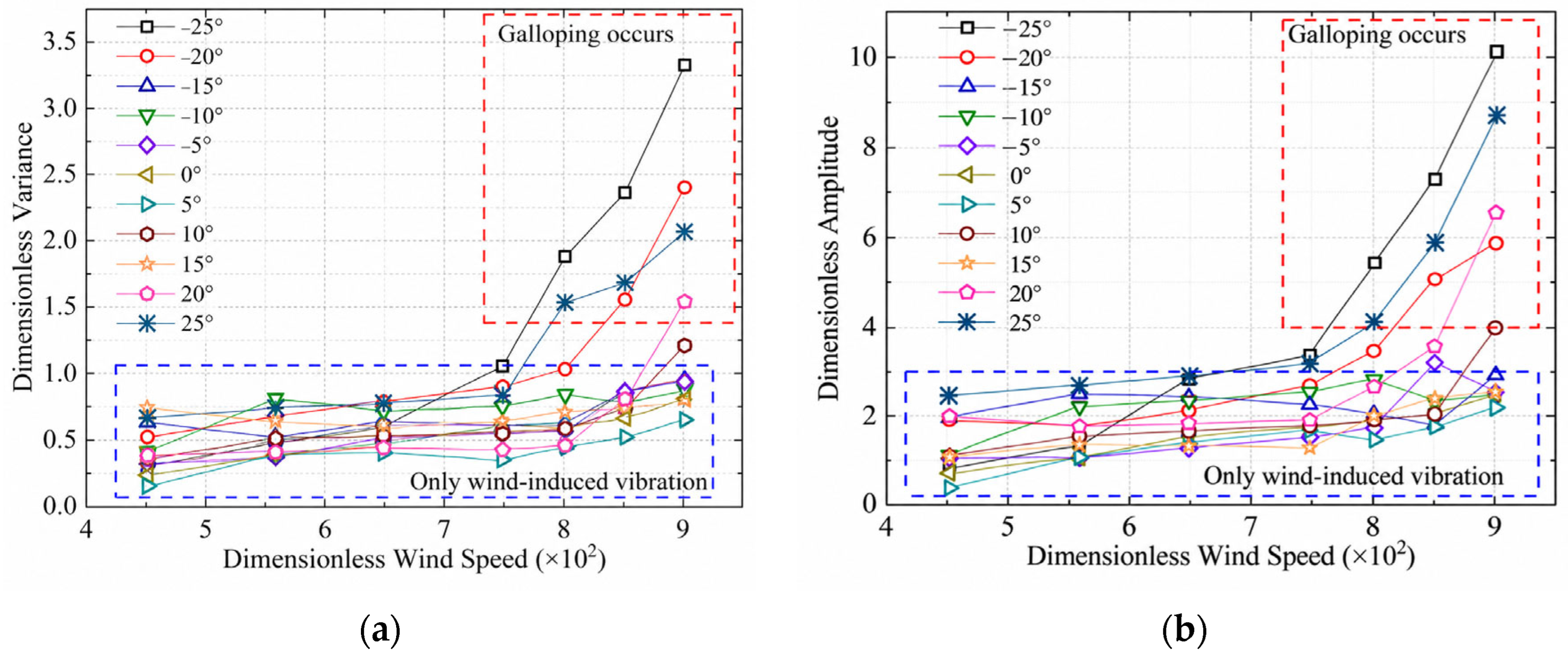
Figure 17 presents the dimensionless variance and dimensionless vibration amplitude obtained from the wind-tunnel tests of the iced auxiliary-conductor model. The dimensionless variance characterizes the randomness of the conductor vibration and the variation in vibration energy distribution; a larger value indicates a stronger vibration response and a greater tendency toward instability. The dimensionless vibration amplitude represents the average vibration magnitude of the conductor and reflects the overall intensity of the vibration; a higher value indicates a more pronounced vibration response and a greater risk of instability.

Figure 17. Wind-tunnel test results. (a) Dimensionless variance; (b) dimensionless vibration amplitude.

As the dimensionless wind speed increases, both the dimensionless variance and vibration amplitude generally exhibit an upward trend, although the response characteristics vary markedly with icing angle. At relatively low wind speeds, all cases remain in a small-amplitude wind-induced vibration regime. With further increases in wind speed, the responses at −25°, −20°, and 25° increase rapidly, indicating a transition toward large-amplitude galloping, with the −25° case showing the most pronounced instability. In contrast, the responses at the remaining icing angles increase more gradually and remain comparatively limited. This pronounced angular dependence is associated with the asymmetric aerodynamic characteristics of the iced cross-section. At unfavorable icing orientations, the asymmetry of flow separation and surface pressure distribution becomes more significant, leading to larger fluctuations in aerodynamic forces during conductor motion. As a result, the aerodynamic energy transferred to the structure increases. When this energy input exceeds the energy dissipated through structural damping, the vibration response is amplified and develops into galloping. These results confirm the strong sensitivity of galloping behavior to both wind speed and icing angle.

In both the simulations and wind-tunnel tests, the iced conductor exhibits relatively small responses at lower wind speeds, followed by a rapid increase in vibration response as the wind speed increases and the system approaches the galloping regime. In particular, the 25° icing-angle condition, which was considered in both the numerical simulations and the wind-tunnel tests, shows a clear increase in vibration intensity with increasing wind speed. The consistent transition from small-amplitude wind-induced vibration to large-amplitude galloping demonstrates that the numerical model can reasonably reproduce the main dynamic characteristics of the iced auxiliary conductor.

The parametric icing results indicate that wind speed, ambient temperature, liquid water content, and droplet size can serve as environmental indicators for assessing the tendency and severity of ice accretion. In particular, conditions associated with increased ice thickness or an expanded icing region may warrant enhanced inspection of auxiliary conductors in icing-prone railway sections. In addition, the galloping results show that aerodynamic instability is strongly related to wind speed and icing angle, with the −25°, −20°, and 25° icing-angle cases exhibiting markedly amplified responses once the critical dimensionless wind speed is exceeded. Therefore, combined monitoring of meteorological conditions, conductor icing state, and vibration response may help identify potentially unstable conditions before severe galloping develops. From the perspectives of maintenance and design, the identified high-risk conditions can provide a basis for prioritizing de-icing operations, inspecting suspension components and conductor condition, and applying or optimizing anti-galloping measures. These findings thus establish a link among environmental icing conditions, conductor dynamic stability, and practical risk management of railway overhead contact systems.

4. Conclusions

This study focuses on auxiliary conductors in electrified railway overhead contact systems and develops a numerical analysis framework encompassing supercooled-water-droplet impingement, heat and mass transfer, ice-shape evolution, and two-way fluid–structure interaction of iced conductors. The galloping response was further validated through wind-tunnel tests. The study clarifies the effects of environmental parameters on the ice morphology of auxiliary conductors, as well as the influences of ice shape, wind speed, and angle of attack on conductor galloping. The findings provide a reference for icing-risk assessment, condition monitoring, maintenance planning, and anti-galloping design of auxiliary conductors in railway overhead contact systems operating in cold and windy regions. The main conclusions are as follows:

(1)

Ice accretion on the auxiliary conductor initially concentrates at the leading edge of the windward surface and gradually extends toward the upper and lower sides of the conductor over time. Increasing wind speed enhances both droplet collision efficiency and icing coverage. Increasing droplet diameter primarily strengthens the inertial effect, causing the icing region to extend farther toward both sides. Increasing liquid water content mainly increases the ice-layer thickness, while having only a limited influence on the icing limits. Decreasing ambient temperature accelerates droplet freezing and results in more concentrated ice accumulation on the windward side.

(2)

Ice accretion markedly reduces the aerodynamic stability of the auxiliary conductor. The bare circular conductor mainly exhibits transient vibrations that gradually decay at wind speeds of 10–20 m/s and eventually stabilizes near its equilibrium position. In contrast, 10 mm crescent-shaped ice accretion disrupts the aerodynamic symmetry of the cross-section and induces sustained periodic galloping. As the wind speed increases, both the galloping amplitude and the rate of response development increase significantly, while the vibration mode gradually evolves from vertically dominated motion into large-amplitude coupled horizontal–vertical motion.

(3)

The wind-tunnel results show that both the dimensionless variance and dimensionless vibration amplitude of the iced auxiliary conductor increase with wind speed and exhibit pronounced sensitivity to the icing angle of attack. Once the dimensionless wind speed exceeds the critical value, the responses under the −25°, −20°, and 25° conditions increase rapidly, and the conductor gradually transitions from small-amplitude wind-induced vibration to galloping. Among these cases, the −25° condition is the most unfavorable, followed by the −20° and 25° conditions. The experimental and numerical results show consistent trends, thereby confirming the rationality of the proposed numerical model.

References

- Zhao, C.; Wang, T. Wind tunnel experimental investigation on the performance of the ice-melting system for high-speed train bogies. Transp. Saf. Environ. 2025, 7, tdae022. [Google Scholar] [CrossRef] [Scilit]
- Zhang, J.; Huang, F. An external design for performance improvement of the transition windbreak wall between an embankment and a hill cut on a high-speed railway. Transp. Saf. Environ. 2025, 7, tdaf010. [Google Scholar] [CrossRef] [Scilit]
- Zhang, W.; Zou, D. Review of pantograph and catenary interaction. Front. Mech. Eng. 2018, 13, 311–322. [Google Scholar] [CrossRef] [Scilit]
- Wang, X.; Chen, L. Analysis of Contact Wire Ablation Under Dynamic Pantograph-Rigid Catenary Separation in Electric Railways. Prot. Control Mod. Power Syst. 2026, 11, 196–208. [Google Scholar] [CrossRef] [Scilit]
- Li, Z.; Huang, G. Prediction model for icing growth characteristics of high-speed railway contact lines. Cold Reg. Sci. Technol. 2024, 227, 104306. [Google Scholar] [CrossRef] [Scilit]
- Lu, G.; Tsang, C.W. Interpretable fault diagnosis for overhead lines with covered conductors: A physics-informed deep learning approach. Prot. Control Mod. Power Syst. 2025, 10, 25–39. [Google Scholar] [CrossRef] [Scilit]
- Zhang, W.; Wang, W. Research on video monitoring technology for galloping of OCS additional conductors of high-speed railway in strong wind zone. Sensors 2024, 24, 7521. [Google Scholar] [CrossRef] [Scilit] [PubMed]
- Chen, S.; Xu, Y. A Robust Estimation Method for the Coupling Matrix in Non-Contact Measurement of Switching Transient Voltages in 500 kV Transmission Lines. Prot. Control Mod. Power Syst. 2026, 11, 159–174. [Google Scholar] [CrossRef] [Scilit]
- Makkonen, L. Modeling of ice accretion on wires. J. Appl. Meteorol. Climatol. 1984, 23, 929–939. [Google Scholar] [CrossRef] [Scilit] [PubMed]
- Makkonen, L. Models for the growth of rime, glaze, icicles and wet snow on structures. Philos. Trans. R. Soc. A Math. Phys. Eng. Sci. 2000, 358, 2913–2939. [Google Scholar] [CrossRef] [Scilit]
- Makkonen, L. Estimation of wet snow accretion on structures. Cold Reg. Sci. Technol. 1989, 17, 83–88. [Google Scholar] [CrossRef] [Scilit]
- Fu, P.; Farzaneh, M. Two-dimensional modelling of the ice accretion process on transmission line wires and conductors. Cold Reg. Sci. Technol. 2006, 46, 132–146. [Google Scholar] [CrossRef] [Scilit]
- Niu, S.; Zhou, Y. The microphysics of ice accretion on wires: Observations and simulations. Sci. China Earth Sci. 2012, 55, 428–437. [Google Scholar] [CrossRef] [Scilit]
- Lébatto, E.B.; Farzaneh, M. Conductor icing: Comparison of a glaze icing model with experiments under severe laboratory conditions with moderate wind speed. Cold Reg. Sci. Technol. 2015, 113, 20–30. [Google Scholar] [CrossRef] [Scilit]
- Zhang, J.; Makkonen, L. A 2D numerical study on the effect of conductor shape on icing collision efficiency. Cold Reg. Sci. Technol. 2017, 143, 52–58. [Google Scholar] [CrossRef] [Scilit]
- Xu, F.; Li, D. Numerical simulation of two-dimensional transmission line icing and analysis of factors that influence icing. J. Fluids Struct. 2023, 118, 103858. [Google Scholar] [CrossRef] [Scilit]
- Han, X.; Wang, J. Collision characteristics of water droplets in icing process of insulators. Electr. Power Syst. Res. 2022, 212, 108663. [Google Scholar] [CrossRef] [Scilit]
- Qing, H.; Jian, Z. Rime icing on bundled conductors. Cold Reg. Sci. Technol. 2019, 158, 230–236. [Google Scholar] [CrossRef] [Scilit]
- Huang, Y.; Chen, Y. Study on icing characteristics of bundled conductor of transmission line based on shadowing effect analysis. Cold Reg. Sci. Technol. 2025, 231, 104393. [Google Scholar] [CrossRef] [Scilit]
- Zarnani, A.; Musilek, P. Learning to predict ice accretion on electric power lines. Eng. Appl. Artif. Intell. 2012, 25, 609–617. [Google Scholar] [CrossRef] [Scilit]
- Sun, W.; Wang, C. Staged icing forecasting of power transmission lines based on icing cycle and improved extreme learning machine. J. Clean. Prod. 2019, 208, 1384–1392. [Google Scholar] [CrossRef] [Scilit]
- Hao, Y.; Yao, Z. A classification method for transmission line icing process curve based on hierarchical k-means clustering. Energies 2019, 12, 4786. [Google Scholar] [CrossRef] [Scilit]
- Chen, Y.; Fan, J. PR-KELM: Icing level prediction for transmission lines in smart grid. Future Gener. Comput. Syst. 2020, 102, 75–83. [Google Scholar] [CrossRef] [Scilit]
- Zhao, J.; Zhang, H. Probability prediction method of transmission line icing fault based on adaptive relevance vector machine. Energy Rep. 2022, 8, 1568–1577. [Google Scholar] [CrossRef] [Scilit]
- Snaiki, R.; Jamali, A. A metaheuristic-optimization-based neural network for icing prediction on transmission lines. Cold Reg. Sci. Technol. 2024, 224, 104249. [Google Scholar] [CrossRef] [Scilit]
- Zhou, R.; Zhang, Z. Reliable monitoring and prediction method for transmission lines based on FBG and LSTM. Adv. Eng. Inform. 2024, 62, 102603. [Google Scholar] [CrossRef] [Scilit]
- Wang, F.; Lin, H. Transmission line icing prediction based on dynamic time warping and conductor operating parameters. Energies 2024, 17, 945. [Google Scholar] [CrossRef] [Scilit]
- Wang, F.; Ma, Z. Transmission line icing prediction based on physically guided fast-slow transformer. Energies 2025, 18, 695. [Google Scholar] [CrossRef] [Scilit]
- Stickland, M.; Scanlon, T. An investigation into the aerodynamic characteristics of catenary contact wires in a cross-wind. Proc. Inst. Mech. Eng. Part F J. Rail Rapid Transit 2001, 215, 311–318. [Google Scholar] [CrossRef] [Scilit]
- Stickland, M.; Scanlon, T. An investigation into the mechanical damping characteristics of catenary contact wires and their effect on aerodynamic galloping instability. Proc. Inst. Mech. Eng. Part F J. Rail Rapid Transit 2003, 217, 63–71. [Google Scholar] [CrossRef] [Scilit]
- Chabart, O.; Lilien, J.L. Galloping of electrical lines in wind tunnel facilities. J. Wind Eng. Ind. Aerodyn. 1998, 74–76, 967–976. [Google Scholar] [CrossRef] [Scilit]
- Zhou, L.; Yan, B. Study on galloping behavior of iced eight-bundle conductor transmission lines. J. Sound Vib. 2016, 362, 85–110. [Google Scholar] [CrossRef] [Scilit]
- Fan, S.; Song, Y. Anti-galloping spoiler deployment for suppressing galloping of overhead contact line in electrified railways. Mech. Mach. Theory 2026, 221, 106371. [Google Scholar] [CrossRef] [Scilit]
- Song, Y.; Zhang, M. A response spectrum analysis of wind deflection in railway overhead contact lines using pseudo-excitation method. IEEE Trans. Veh. Technol. 2021, 70, 1169–1178. [Google Scholar] [CrossRef] [Scilit]
- Song, Y.; Wang, Z. A spatial coupling model to study dynamic performance of pantograph-catenary with vehicle-track excitation. Mech. Syst. Signal Process. 2021, 151, 107336. [Google Scholar] [CrossRef] [Scilit]
- Sugahara, A.; Yamashita, C. Improvement of anti-fatigue property of contact wire by modifying cross-section shape. Q. Rep. RTRI 2013, 54, 31–38. [Google Scholar] [CrossRef] [Scilit]
- Wang, X.; Song, Y. A time-frequency dual-domain deep learning approach for high-speed pantograph–catenary dynamic performance prediction. Mech. Syst. Signal Process. 2025, 238, 113258. [Google Scholar] [CrossRef] [Scilit]
- Chen, S.; Song, Y. Defects detection for railway catenary system with encoder-decoder architecture. Railw. Eng. Sci. 2025, 34, 528–552. [Google Scholar] [CrossRef] [Scilit]
- Amano, Y.; Kobayashi, S. Mechanism and suppression of friction-induced vibration in catenary-pantograph system. Nonlinear Dyn. 2024, 112, 14959–14980. [Google Scholar] [CrossRef] [Scilit]
- Amano, Y.; Kobayashi, S. Effects of periodic structures on friction-induced vibrations in catenary-pantograph systems. Tribol. Int. 2025, 203, 110406. [Google Scholar] [CrossRef] [Scilit]
- Liu, C.; Zhang, Y. Numerical simulation and analysis of the influencing factors of ice formation on electrified railway contact lines. Infrastructures 2025, 10, 121. [Google Scholar] [CrossRef] [Scilit]
Disclaimer/Publisher’s Note: The statements, opinions and data contained in all publications are solely those of the individual author(s) and contributor(s) and not of MDPI and/or the editor(s). MDPI and/or the editor(s) disclaim responsibility for any injury to people or property resulting from any ideas, methods, instructions or products referred to in the content. |
© 2026 by the authors. Licensee MDPI, Basel, Switzerland. This article is an open access article distributed under the terms and conditions of the Creative Commons Attribution (CC BY) license.