


Abstract
As urban rail transit systems enter a stage of high-quality development, accurate short-term passenger flow forecasting has become essential for efficient operation and management. To improve the accuracy and robustness of multi-step short-term passenger flow forecasting under fluctuating demand conditions, this study develops a feature-enhanced Informer framework that embeds Complex Network Representation (CNR) into the Informer architecture to jointly capture both the topological characteristics of the subway network and spatiotemporal passenger flow dynamics. External factors, including subway schedules and land use around stations, are further integrated to enrich the input features. In addition, the ProbSparse self-attention mechanism is adopted to improve long-sequence dependency modeling, thereby enabling efficient multi-step passenger flow forecasting. Experiments were conducted on the Beijing metro passenger flow dataset from January to October 2024 to evaluate the proposed model. The dataset covered 264 stations and was aggregated at 15 min intervals. Based on historical passenger flow and multi-source features, the model predicts passenger flow over multiple future time steps. The overall evaluation metrics were calculated on the test set and averaged over all test samples and observed stations. The experimental results show that, compared with the standard Transformer model, the proposed model reduces the average prediction error by 16.59% on weekdays and 20.48% on weekends while maintaining stable predictive performance during peak hours. Sensitivity analysis and ablation studies are further conducted to evaluate the model performance across different station types and forecasting horizons. The results demonstrate that the proposed model can provide reliable decision support for intelligent urban rail transit operations, including transport capacity scheduling, passenger service improvement, and operating cost reduction.
1. Introduction
Urban rail transit, as the backbone of modern urban transportation systems, is experiencing rapid development worldwide. As of 2024, 58 cities in mainland China have launched rail transit systems, with a total operating length exceeding 12,000 km and an average daily ridership surpassing 5 million passengers [1]. Its development not only mitigates urban traffic congestion but also reshapes urban mobility ecosystems, owing to its high capacity, punctuality, and low carbon emissions. For instance, the Guangzhou Subway has established and opened 23 lines, covering over 1000 km, with a record daily ridership of 12.2 million passengers, making it one of the busiest subway networks in the world. The integration of four intercity railways has led to a 209.7% increase in average daily passenger flow, promoting seamless connectivity among subway, intercity, high-speed, and suburban rail systems and advancing the development of rail-based urban agglomerations [2].
Rail transit systems have become the cornerstone of smart city urban efficiency due to systematic, intensive, and sustainable characteristics. Their high-capacity rapid commuting capability is irreplaceable [3,4]. A single subway train can transport over 2000 passengers per hour during peak times—more than 10 times the capacity of buses. In addition, schedule precision and reliability foster commuter trust. With exclusive right-of-way, urban rail systems maintain all-weather punctuality, significantly outperforming road-based transport vulnerable to traffic conditions [5,6]. The subway contributes to urban carbon emission reduction and aligns with green development. Electrically powered systems dramatically reduce emissions, with energy consumption per passenger being merely 1/10 of that of private cars and 1/3 of buses. On a deeper level, rail transit contributes to the restructuring of urban space. Through Transit-Oriented Development (TOD), it promotes intensive land use and helps shape multi-centered urban structures [7,8].
Currently, research on urban rail transit passenger flow prediction mainly refers to predicting the passenger volume within a certain scope over a unit of time. Passenger flow forecasts can be classified into boarding passenger flow prediction, outbound passenger flow prediction, and transfer flow prediction, depending on different passenger travel behaviors. From the perspective of prediction duration, predictions can be divided into long-term, mid-term, and short-term forecasts based on the time unit considered [3,4]. Long-term and mid-term passenger flow prediction in urban rail transit is often influenced by macro-level factors such as national economic development, changes in transportation structure, population growth, and government policies, making these types of prediction more challenging. Due to the high randomness and volatility of urban rail transit passenger flow, short-term prediction is generally focused on in practice. Short-term passenger flow prediction refers to using historical passenger flow data to extract flow patterns and predict passenger volumes over one or multiple upcoming time intervals [9].
With urbanization, growing demand for public transportation, and the continuous innovation of artificial intelligence (AI) technology, artificial intelligence is playing an increasingly vital role in urban rail transit passenger flow prediction. By leveraging AI algorithms such as deep learning and graph neural networks (GNNs), the module can extract passenger travel patterns and spatiotemporal characteristics from large-scale rail transit data. Complex topological features reflect the spatial relationships between different stations, while spatiotemporal characteristics reveal the dynamic patterns of passenger flow over time [10]. AI can integrate multi-source heterogeneous data, such as historical passenger flow, weather conditions, and holiday information, to construct prediction models, thereby improving the prediction accuracy and monitoring of real-time passenger flow [11,12]. This study proposes a Complex Network Representation integrated Informer (CNR-Informer) model for multi-step short-term passenger flow prediction in urban rail transit. Based on complex network representation, we constructed metrics to analyze the spatiotemporal features of subway passenger flow and develop an Informer neural network for multi-step short-term prediction.
Although graph neural networks, graph attention mechanisms, and Transformer-GNN models have been widely applied to urban rail transit passenger flow prediction and have achieved good performance in capturing spatiotemporal dependencies among stations, most existing methods mainly rely on adjacency matrices, distance relationships, or data-driven implicit graph structures to learn spatial correlations. As a result, insufficient attention has been paid to the structural roles of stations in the rail transit network and their transportation interpretations. In practice, stations differ substantially in terms of network connectivity, hub function, transfer intermediary role, local clustering characteristics, and inbound–outbound passenger flow balance. These differences further affect the aggregation, diffusion, and fluctuation of passenger flows. Therefore, it is necessary to introduce complex network representations with explicit transportation interpretations into the spatiotemporal prediction framework. This can address the limitations of conventional graph structures in representing station-level functional heterogeneity and network structural effects while enhancing the model’s ability to capture passenger flow dynamics across different types of stations.
The main contributions are as follows: First, we develop the CNR-Informer network based on feature enhancement, employing an encoder–decoder structure to enable multi-step passenger prediction. Second, the complex network metrics are designed to extract network structural attributes and dynamic passenger flow fluctuation. Train schedules, station accessibility, and point of interest (POI) data are considered for precise predictions. Third, the ProbSparse Attention mechanism is integrated to extend the model’s capability in handling longer spans of subway passenger flow data, which allows for capturing long-term trends and cyclic variations, ultimately boosting the accuracy of predictions.
2. Literature Review
2.1. Spatiotemporal Passenger Flow Characteristics of Urban Rail Transit
Passenger travel records constitute vital information that captures the temporal dynamics and spatial patterns of urban mobility. These multidimensional datasets provide critical insights for optimizing transportation network design, enhancing demand prediction models, and implementing adaptive scheduling strategies. The observed mobility patterns reveal intricate supply–demand interdependencies that evolve through the synergistic effects of socioeconomic, environmental, and operational factors. Specifically, urban rail systems demonstrate pronounced spatiotemporal heterogeneity in passenger flow distributions: Temporally, weekday operations exhibit characteristic bimodal distributions with distinct morning (7–9 AM) and evening (5–7 PM) rush-hour peaks, while holiday patterns tend toward unimodal or plateaued distributions. Empirical data from the Beijing Subway illustrates this temporal variance, with peak-hour passenger volumes reaching 2–3 times the baseline levels during morning commutes [4]. Spatially, flow concentrations emerge along arterial corridors linking commercial CBDs, intermodal transit hubs, and high-density residential clusters. These mobility patterns demonstrate complex temporal scaling characteristics, manifesting as seasonal fluctuations, e.g., Lunar New Year migration surges and stochastic perturbations induced by exogenous shocks, including meteorological extremes and public health emergencies [3].
With the popularization of spatiotemporal big data, Smart Card Data (SCD) are increasingly being used in data mining to analyze transportation patterns. Kusakabe and Asakura proposed a data fusion method that combines smart card system data with individual travel survey data. They used a Naive Bayes classifier to infer travel purposes and mined passenger behavioral characteristics to assist transportation operators in behavior monitoring and analysis [13]. Qi et al. proposed a method combining constrained fuzzy C-means clustering, non-negative tensor factorization, and artificial neural networks. They utilized smart card data and POI data from Beijing to uncover patterns of regional passenger mobility on public transit. This method effectively mines regional commuting patterns and tidal mobility patterns. Integrating features of boarding and alighting behaviors further enhances the accuracy of cluster pattern prediction [14]. Alsger et al. conducted passenger activity mining on time and spatial attributes using multiple data sources. They set thresholds for activity duration and start time to discover regular OD trips and infer activities related to work and home. Huang constructed a research framework to track individual residential and work dynamics based on 7 years of transportation smart card data. They analyzed the evolution of individuals’ behaviors, studied their commuting time and housing expenses to analyze their work and housing patterns, and concluded that a 45 min commuting time is a turning point in behavioral preference changes [15].
Land use patterns and functional layouts serve as fundamental driving forces influencing urban rail transit. Using Guangzhou as a case study, Li et al. integrated multi-source spatial big data, including remote sensing imagery, points of interest (POI), and social media data, to construct a Geographically Weighted Regression (GWR) model. Their analysis revealed spatial heterogeneity in the relationship between rail transit ridership and the built environment. By combining the GWR coefficients with k-means clustering, they classified transit stations into distinct groups and proposed differentiated zoning policies aimed at enhancing rail transit usage through targeted interventions in the built environment [16]. Ding et al. applied a Gradient Boosting Decision Tree model to examine how characteristics of the built environment surrounding subway stations influence daily passenger volumes [17]. Huang et al. employed a Bayesian network learning approach to explore the causal relationships between built environment features in Transit-Oriented Development (TOD) areas and subway ridership [18]. Hagenauer et al. conducted a comparative analysis of travel mode choice modeling using seven machine learning classifiers, finding that the Random Forest algorithm exhibited superior predictive performance [19].
The topological structure of urban rail transit networks plays a crucial role in travel demand prediction. Factors such as line coverage, transfer convenience, and operational reliability directly affect passengers’ route and mode choices. Topological characteristics, including node degree distribution, betweenness centrality, and path redundancy, further influence passenger travel efficiency and the spatial distribution of demand. For example, ring-shaped networks can help balance passenger flows by providing multiple route alternatives, whereas radial networks are more likely to experience overloading at core hubs. Stations with high betweenness centrality, such as major transfer hubs, usually carry large volumes of inter-regional passenger flows and may become potential bottlenecks, thereby weakening network robustness. To extract the spatial topological features of rail transit networks, Yin et al. regarded each rail transit line as an independent network layer and constructed a multilayer directed weighted network model. They proposed a comprehensive set of structural indicators, including node degree, betweenness centrality, and node efficiency, to quantitatively characterize network topology [20]. Based on complex network theory, Xiao et al. modeled the Beijing rail transit system as a directed and dynamically weighted network, in which edge weights were represented by sectional passenger volumes. By constructing a local dynamic indicator distribution model, they revealed the intrinsic relationship between network vulnerability and heterogeneity, thereby supporting the identification of critical nodes [21]. Xu et al. investigated the temporal evolution of resilience indicators associated with topological features and passenger flow patterns. Their case study of the Hong Kong metro system showed that optimized resource allocation and a denser distribution of subway stations can significantly enhance system resilience to service disruptions [22]. Xu et al. further constructed a directionally weighted passenger flow network and analyzed individual travel activity patterns from the perspectives of passenger flow distribution, temporal characteristics, and hierarchical clustering structures. Their results indicated that the concentration of urban activities leads to highly heterogeneous spatial flow patterns and passenger volumes [23].
2.2. Multi-Step Short-Term Passenger Flow Prediction
Existing short-term passenger flow prediction methods can be primarily categorized into three types: statistical models, machine learning, and deep learning-based prediction models [9]. Initially, short-term passenger flow prediction relied on traditional mathematical and statistical models, such as the Historical Average (HA) model, the least squares method, ARIMA, and the logistic regression model. Traditional statistical prediction models, like the Autoregressive Integrated Moving Average (ARIMA) and its variants (e.g., Seasonal ARIMA, SARIMA), have fixed model complexity and limited parameters, constraining their ability to fit entire time series and capture nonlinear features in the data. Tang et al. proposed time-series models, ARIMA, linear regression, and support vector regression (SVR) under weather influence factors based on the Automatic Fare Collection (AFC) system to predict short-term passenger flow [24]. Wang et al. utilized the Seasonal ARIMA (SARIMA) model to capture the inherent periodic characteristics of passenger flow and combined it with a Support Vector Machine (SVM) to construct a locally online SVM model. By embedding nonlinear features, they achieved accurate predictions for unstable weekend and holiday passenger flows [25].
Machine learning-based models such as K-Nearest Neighbor (KNN), Support Vector Machines (SVMs), and neural networks have demonstrated strong capabilities in capturing uncertainty and nonlinear patterns in passenger flow fluctuations. These models offer innovative solutions to the limitations of traditional mathematical models in handling stochasticity. However, they are still constrained by the shallow representation of features. Dinh et al. developed a short-term traffic flow prediction model based on SVM and compared its performance with several baseline methods, including Historical Averages, current-time-based predictions, and double exponential smoothing. The results showed that for most prediction intervals and under varying traffic conditions, the SVM model outperformed the baselines when using a 30 min rolling window. Moreover, as the rolling horizon extended from 30 to 60 min, the predictive accuracy of the SVM model further improved [26]. Zou et al. proposed using the eXtreme Gradient Boosting (XGBoost) model to identify the contribution of different variables to passenger flow prediction. Compared to benchmark models, XGBoost significantly improved both prediction accuracy and computational efficiency on real-world datasets [27]. Despite the evident advantages of machine learning-based hybrid models over traditional statistical approaches in prediction rail transit passenger flows, two key limitations remain in their practical deployment. First, many models exhibit high time complexity, making it difficult to meet the real-time response requirements of short-term passenger flow prediction, especially in scenarios involving minute-level data updates. Second, current models often fail to fully capture multi-scale spatiotemporal dependencies. This limitation becomes particularly pronounced in large-scale transit systems (e.g., those with 200+ stations). Their ability to represent complex spatiotemporal dependencies, such as inter-station passenger flow propagation and networked trip chains, remains limited, leading to higher prediction errors across the entire network.
Deep learning neural networks with more hidden layers capture more dimensional data features and complex data relationships. Recurrent Neural Networks (RNNs) are generally used to model the temporal dependencies of data, but the inherent design flaws of standard RNNs may lead to issues such as gradient vanishing and explosion when handling long sequences, making model training difficult. In recent years, deep learning technology has demonstrated significant advantages in the field of urban rail transit passenger flow prediction, primarily by efficiently capturing the spatiotemporal correlations of passenger flow data through multilayer nonlinear structures. Mainstream models often adopt a hybrid architecture of Long Short-Term Memory networks (LSTM) and Graph Convolutional Networks (GCNs), where the former is used to model long-term dependencies in time series and the latter extracts spatial features by constructing inter-station topology graphs [9]. Prediction models based on the LSTM framework can address these issues and achieve more accurate passenger flow predictions. Gated Recurrent Units (GRUs), by simplifying the gate structure of LSTM and reducing network parameters, effectively improve training efficiency. Vaswani et al. proposed the Transformer architecture, which established a feature extraction pattern entirely based on self-attention mechanisms [28]. In time-series prediction tasks, through dynamic weight allocation mechanisms, Transformer achieved modeling of long-term dependencies in multivariate time-series data. Some researchers have applied Transformer to the field of passenger flow prediction and obtained promising results. However, these models often focus on a single-time granularity, overlooking the cross-scale correlation characteristics of multi-granularity data. Wang Z J et al. established a combination prediction model EMD-LSTM based on Empirical Mode Decomposition (EMD) and LSTM. EMD is used to extract the trend of passenger flow changes, and LSTM is utilized for prediction. Experimental results show that the EMD-LSTM model outperforms the standalone LSTM model in terms of prediction accuracy [29]. Li et al. employed the Matching Pursuit Orthogonal Least Squares algorithm and proposed a new multiscale radial basis function network, achieving high-precision predictions for irregular demands and accurately locating affected subway stations [30]. Hao et al. introduced an end-to-end deep learning framework capable of multi-step predictions for all stations in a large-scale subway system simultaneously [31]. Jia et al. presented a hybrid model based on deep learning that combines Long Short-Term Memory neural networks with stacked autoencoders to simultaneously predict short-term passenger flows at various stations within the subway network [32]. Xiong et al. utilized two deep learning models, Long Short-Term Memory neural networks and Convolutional Neural Networks, to capture the temporal and spatial features of urban rail transit passenger flow, achieving accurate results for both long-term and short-term predictions of passenger flow [33].
In the prediction of urban rail transit passenger flow, traditional deep learning methods such as LSTM, GRU, and Transformer have made some progress, but they still have significant limitations in practical applications. These methods still have shortcomings when dealing with a long series of passenger flow data. Neural network structures like LSTM and GRU are limited by the recursive calculation paradigm of sequence modeling. When capturing periodic passenger flow patterns lasting for weeks or even months, they are prone to issues such as gradient vanishing, information decay, and weak parallel computing capabilities [34]. On the other hand, the Transformer overcomes the sequence length limitation with its self-attention mechanism, but the quadratic complexity of its computation leads to high memory usage and low training efficiency when handling high-frequency (e.g., 10 min granularity) long-term passenger flow data. Especially in urban rail transit scenarios, sudden changes in passenger flow patterns triggered by external factors like holidays and weather are difficult to effectively capture by the standard attention mechanism. In comparison, the emerging Informer model utilizes the ProbSparse self-attention mechanism, significantly reducing computational complexity. It can efficiently handle ultra-long time-series data, strengthen the identification ability of key time points in passenger flow sequences, and avoid the issue of error accumulation in traditional methods, which demonstrates stronger application potential in complex and dynamically changing urban rail transit scenarios [35].
Existing graph-based and Transformer-GNN prediction models have achieved good performance in capturing the spatiotemporal dependencies of passenger flow. However, their spatial representations often lack explicit interpretations of transportation attributes, such as station connectivity, hub importance, transfer intermediary function, and passenger flow imbalance. Current studies on urban rail transit passenger flow prediction still face several limitations. First, the explicit representation of network topology and station functional heterogeneity remains insufficient. Many models mainly rely on historical passenger flow series or adjacency-based spatial relationships, but they pay limited attention to station-level topological roles, such as transfer hubs, terminal stations, and highly accessible stations. The influence of network structure on passenger flow generation, attraction, and transfer is not fully captured. Second, the propagation of passenger flow fluctuations across the rail transit network has not been adequately described. Passenger flow changes may spread through route choice, transfer behavior, and line-level operational connections, especially during peak hours, weekends, or event-driven demand surges. Existing spatiotemporal models still have limited ability to capture these network-related fluctuation patterns. Third, although Transformer-based models are effective for long-sequence prediction, they may lack explicit network structural information and external contextual support. This limits their ability to explain passenger flow differences across stations, lines, and day types. In addition, network topology, train operation, station accessibility, POI characteristics, and weather conditions are often not integrated into a unified representation framework. Unlike existing graph-based and Transformer-GNN models that mainly rely on adjacency relationships or graph propagation mechanisms to learn spatial dependencies, this study introduces complex network indicators with explicit transportation interpretations to characterize the structural roles of different stations in the rail transit network and their influence on passenger flow evolution.
3. Method
3.1. Complex Network Topological Features of Urban Rail Transit
This study constructs a complex network topology model for urban rail transit and measures the topological complexity of the network using relevant metrics of complex networks. The metrics are divided into two major categories: node feature metrics and network structure metrics. Node feature metrics primarily reflect the topological characteristics of nodes or edges in the network, with commonly used measures including node degree, betweenness, clustering coefficient, etc. Network structure metrics are used to describe the overall topological properties of the network, with commonly used measures such as degree distribution and global clustering coefficient [36].
Based on user travel records data from the urban rail transit network, a travel network is constructed, where the nodes in the travel network represent the entry and exit stations, and trips from origin to destination are considered as edges between nodes. A directed weighted network is constructed, where denotes the set of nodes, with N being the total number of stations in the network; represents the edges between adjacent stations in the urban rail transit network.
Node degree is a fundamental metric used to quantify the importance of the node. The degree of node represents the number of edges directly connected to it. The calculation of is given by Equation (1), where indicates whether a link exists between node and node : if the edge exists, and 0 otherwise.
Similarly, we define the strength of node to describe the intensity of passenger flow between nodes, as shown in Equation (2). Here, represents the OD (origin-destination) passenger flow volume between node and node .
The betweenness centrality is used to evaluate a node’s influence within the entire network. The betweenness centrality of a node is defined as the ratio of the number of shortest paths between all node pairs in the network to the number of those paths that pass through node . The calculation of is shown in Equation (3). denotes the total number of shortest paths from node to node , while indicates the number of those paths that pass through node . In urban rail transit networks, a station’s betweenness centrality reflects its significance as a “transfer hub” for trips between any two other stations, indicating the station’s structural influence within the network. A higher betweenness centrality value suggests that a greater number of trips throughout the network require passing through that station.
The clustering coefficient measures the degree of interconnection between a node’s neighbors, reflecting the local compactness of the network. In urban rail transit networks, the clustering coefficient can be used to assess the connectivity among a station’s neighboring stations, indicating the degree of local aggregation and redundancy of the network. This metric helps analyze the robustness and accessibility of the network. Let represent the set of stations and represent the edges between adjacent stations on the lines. The clustering coefficient of a node is defined as the ratio of the number of existing edges among the neighbors of station to the maximum number of possible edges between them. In Equation (4), is the actual number of connections among the neighbors of node , and is the degree of node . The maximum possible number of edges between neighbors is given by .
The average clustering coefficient of an urban rail transit network is the average of the clustering coefficients of all nodes and is denoted as in Equation (5).
PageRank measures the node importance, originally developed by Google for web page ranking. In the context of urban rail transit networks, PageRank can be used to evaluate the influence of each station, i.e., which stations are more likely to be reached if a passenger starts randomly and transfers probabilistically. A higher PageRank value for a station indicates a greater likelihood that the station will be reached during the passenger travel process, suggesting that the station plays a more important role in the network. is the PageRank value of node , where is the total number of stations in Equation (6). The parameter is the damping factor (typically set to 0.85), representing the probability that a passenger continues traveling. is the total number of stations in the network. is the set of neighboring stations that point to station , i.e., those from which station is directly reachable. is the out-degree of station , i.e., the number of stations reachable from . is the probability that a passenger jumps randomly to any station. Stations with high PageRank values are often important transfer hubs or major passenger flow aggregation areas.
The Net Flow Rate (NFR) is used to analyze the dynamics of passenger flow entering and exiting different stations during various time periods. The calculation method of NFR is shown in Equation (7), where the value of ranges between −1 and 1. The parameters and represent the number of departures and arrivals in station , respectively. When , it indicates that the number of departures exceeds the number of arrivals in the time period, suggesting that more transportation capacity may be needed to meet travel demand. Conversely, if , the number of arrivals exceeds departures in that area, showing a characteristic of passenger flow convergence.
Moran’s I measures spatial autocorrelation, which helps determine whether the spatial distribution of a variable is clustered, dispersed, or random. In urban rail transit networks, Moran’s I can be used to assess the spatial correlation of station passenger flows within the network structure in Equation (8), helping to determine whether stations with high congestion or large passenger volumes are clustered within the network. Here, denotes the number of spatial stations, and represents the weight between station and , determined based on the actual OD passenger flow between them. denotes the sum of all weights in the spatial weight matrix. and denote the passenger flow values at station and , and is the average passenger flow over the observed time period.
The value of Moran’s I ranges from −1 to 1. A Moran’s I value close to 1 indicates positive spatial autocorrelation, meaning that the passenger flow characteristics tend to cluster among adjacent nodes or edges in the urban rail transit network. Conversely, a value close to −1 indicates negative spatial autocorrelation, suggesting that passenger flow characteristics are dispersed among neighboring nodes or edges.
3.2. Transformer Structure for Flow Features Extraction
The Transformer is a deep-learning model based on the self-attention mechanism. It employs multi-head attention layers and distributed GPU parallel computing to enhance training efficiency and model performance. Following a sequence-to-sequence structure, the Transformer processes all elements of the input sequence simultaneously, capturing complex relationships. For long-term time-series prediction, it outperforms traditional sequence models like Long Short-Term Memory (LSTM) and Gated Recurrent Unit (GRU), effectively mitigating issues such as error accumulation. The Transformer adopts an encoder–decoder structure, where the encoder consists of a multi-head self-attention layer followed by a feedforward neural network, as shown in Figure 1. Its unique self-attention mechanism enables the model to capture dependencies between any positions in the sequence, making it more efficient and accurate for long-sequence prediction tasks. Therefore, the Transformer structure excels at modeling long-range dependencies, particularly relationships between distant time points, thereby improving prediction accuracy.
Figure 1.
Transformer network structure.
The input layer of the Transformer includes the embedding layer and the positional encoding layer. Assuming a time-series sequence consists of elements, each with features. The embedding layer plays a crucial role in converting numerical data into vector representations, capturing inter-sequence relationships in a high-dimensional space. To address the inherent limitation of self-attention mechanisms in sequential modeling, the Transformer introduces positional encoding to embed spatiotemporal features. A sine–cosine alternating encoding strategy is employed to achieve position-aware representations of passenger flow sequences. Positional encoding is computed in Equations (9) and (10). denotes the encoded position, providing a unique value for each position and dimension. represents the absolute position index of the passenger flow data. is the dimension index of the encoding vector, and is the feature dimension of the model input. These positional encodings ensure that each position in the passenger flow data has a unique representation, enabling the model to capture sequential information effectively.
Multi-head self-attention enhances the model’s ability to focus on different parts of the input sequence simultaneously. By allocating different weights to segments of input passenger flow data, it can adaptively focus on important parts of the data and learn features of passenger flow data from multiple stations simultaneously through a parallel structure. The attention mechanism in the Transformer model dynamically calculates the correlation weights between different positions in the sequence, enabling the model to flexibly capture long-range dependency relationships, as illustrated in Figure 2. By computing the dot product of Query and Key matrices, it measures the strength of the relationship between position and in the sequence and obtains attention weights through scaling and normalization using Softmax. Here, represent the Query matrix, Key matrix, and Value matrix. The scaling factor prevents the gradient disappearance in Equation (11).
Figure 2.
Multi-head attention mechanism.
The input sequence undergoes three linear transformations to generate the Query matrix, Key matrix, and Value matrix. is the sequence length, and is the feature dimension. Each attention head captures the relational information between input sequences, with the calculation formulas involving learnable parameter matrices , , and in Equation (12). The results from multiple attention heads are concatenated to aggregate the outcomes in Equation (13), ensuring that the model comprehensively considers the results from different attention heads and captures the correlation relationships within the input sequence. Each head has independent matrices , and the concatenated output is then mapped back to the original dimension through .
The output of the multi-head attention mechanism is passed through a feed-forward neural network that uses a nonlinear feature transformation architecture set as a two-layer design in Equation (14). First, we compute the input of the hidden layer using a linear transformation and bias, then apply the ReLU activation function to the hidden layer’s input. Next, the output layer undergoes another linear transformation and bias to produce the final output . Here, is the output of the multi-head self-attention layer. and represent the feature space mapping matrices for the first and second linear transformations, and and are the bias vectors for the two layers, respectively.
3.3. Feature-Enhanced CNR-Informer for Passenger Flow Prediction
Deep neural networks often need to deal with a vast amount of information during the feature-learning process, leading to information overload problems. By utilizing attention mechanisms, it is possible to focus on key information while reducing attention to less relevant details, thereby enhancing the efficiency and accuracy of task processing. Traditional self-attention mechanisms attempt to assign weights to all information, which may result in irrelevant details influencing the output. To address inaccuracies in predicting long input sequences, the Informer assigns higher weights to advantageous features with key characteristics, significantly reducing the dimensionality of input time to extract more critical historical moment information. The Informer structure primarily optimizes efficiency and performance in handling long sequences through the skills of ProbSparse Self-Attention mechanism and the distillation layer.
The overall architecture of the Informer model, as shown in Figure 3, can be divided into four parts: the input layer, output layer, encoder layer, and decoder layer. The left-side encoder is designed for receiving large-scale long sequence inputs, efficiently extracting feature information using the proposed multi-head sparse probability attention mechanism instead of the traditional self-attention mechanism. The encoder layer mainly consists of multiple encoders and distillation layers, with stacked copies enhancing the model’s robustness. On the right side, the decoder structure receives long sequence inputs, including a segment of known sequences before the target time point and zero-filled target sequences. After measuring the weighted attention combination of feature maps through the decoder, a vector is generated for each target sequence position, and the output prediction results are then generated through fully connected layers in a step-wise manner.
Figure 3.
Encoder and decoder structure of the Informer model.
Accurate predictions of passenger volumes over extended periods are essential for schedule adjustments, maintenance planning, and capacity expansions, ultimately leading to a more reliable and responsive urban rail transit system. Long-sequence time-series prediction is crucial, requiring the designed models to possess the capability to handle long-range dependencies. The feature-enhanced CNR-Informer model utilizes the multi-head sparse probability attention mechanism as a key enhancement component. In the self-attention computation process, important query vectors are selected through KL divergence calculation. Specifically, by focusing on the selected query values, the attention interaction is restricted to a specific, optimized range for computation, reducing time complexity and memory usage to optimize computational efficiency. For each query , the dot product with all keys is calculated along with a sparsity score in Equations (15) and (16).
The first term in Equation (16) represents the maximum similarity between the query and all keys, reflecting the peak of attention distribution. The second term is the average similarity between the query and all keys, reflecting the dispersion of attention distribution. A higher value of indicates that the attention distribution of shows higher sparsity, concentrating more on a few keys, and should be retained. Conversely, a lower value of indicates that the attention distribution of is redundant and should be discarded. The sparsity scores for all queries are sorted, and only the top queries (where is a hyperparameter, typically set to 5) with the highest scores are retained. The rows in the attention matrix corresponding to the queries not selected are zeroed out. Attention weights are computed only for the selected queries, where represents the sparse query matrix after filtering in Equation (17).
The encoder design in the Informer architecture relies on self-attention distillation techniques to reduce the input to cascading layers. Distillation layers are inserted between self-attention units, utilizing convolution and max-pooling methods for downsampling operations on features, significantly reducing network size and shortening the input sequence length. The output of the -th layer is as follows:
The CNR-Informer model integrates the complex network topology of urban rail transit with the ProbSparse Self-Attention mechanism and distillation operations to effectively capture long-term temporal dependencies in historical passenger flow data. Therefore, the encoder of the proposed model can efficiently handle extremely long input sequences, enhancing the model’s capability to process long sequences. The generative decoder in Informer can predict the entire long time series at once, rather than step-by-step prediction, significantly improving efficiency during the inference process.
4. Experimental Results
4.1. Exploratory Data Analysis
This study uses passenger flow data from the Beijing urban rail transit system from January to October 2024. The data are collected at 15 min intervals and cover 264 stations in the Beijing metro network. The passenger flow data fields include station ID, station name, time interval, passenger inflow and outflow, and station longitude and latitude. Passenger flow data describe temporal demand variations, while station coordinates are used to construct spatial relationships and network topology. In addition, POI and train timetable data are incorporated to capture the external and operational factors influencing passenger flow variations. POI features, including residential areas, office buildings, commercial facilities, restaurants, and entertainment venues within the service area of each station, are used to characterize surrounding land-use patterns and travel-attraction intensity. Train timetable data, including line information, train arrival and departure times, and service headways, are used to represent the operational service conditions at each station. Specifically, the first 80% of the time-ordered samples are used as the training set, and the remaining 20% are used as the test set. This chronological split ensures that all models are trained only on historical data and evaluated on later observations, which is consistent with the practical forecasting scenario.
Passenger flow at urban rail transit stations exhibits distinct spatial and temporal characteristics [37,38]. Figure 4 illustrates the distribution of entry and exit passenger flow on weekdays and holidays at different stations. Representative stations from the Central Business District (CBD), residential areas, scenic spots, and commercial areas are selected for data analysis. In the CBD and residential areas, passenger flow tends to be lower on holidays, while stations in tourist and commercial areas show a clear increase in passenger flow. As shown in Figure 4a, at Guomao Station in the CBD, there is a significant difference in passenger flow patterns between weekdays and holidays. On weekdays, the station exhibits a clear commuting pattern: from 7:00 to 9:00 AM, outflow peaks at 19,482 passengers per hour, while inflow is only 4240. From 5:00 to 7:00 PM, inflow peaks at 15,209 per hour, and outflow decreases to 4676. As a CBD station, the average hourly inflow and outflow on holidays are 1528 and 1676, respectively. Figure 4b shows the passenger flow at Huilongguan Station, a residential station. On weekdays from 7:00 to 9:00 AM, inflow reaches 5233 per hour, while outflow is only 451. From 5:00 to 7:00 PM, outflow peaks at 4991 per hour. As a residential area station, the average hourly inbound and outbound flows on holidays are 487 and 552, respectively. Figure 4c displays the passenger flow pattern at a scenic spot station. Compared to weekdays, both inflow and outflow increase significantly after 10:00 AM on holidays, with the peak hourly inflow reaching 6952 after 4:00 PM. Figure 4d illustrates the passenger flow at a commercial area station. Surrounded by shopping malls and restaurants, this station experiences high passenger flow on holidays, especially in the evening, when both entry and exit flows increase significantly due to visitor activity.
Figure 4.
Distribution of passenger inflow and outflow at different types of stations on weekdays and holidays. (a) CBD, Guomao Station. (b) Residential area, Huilongguan Station. (c) Scenic spot, Nanluoguxiang Station. (d) Commercial area, Xidan Station.
Figure 5 shows the spatial distribution of hourly entry passenger flow at stations on weekdays and holidays. During holidays, stations with high passenger flow are mainly railway stations, such as Beijing West Railway Station and Beijing Railway Station. In addition, stations located in shopping and tourist areas, such as Wangfujing Station and Nanluoguxiang Station, also experience concentrated high passenger volumes. On weekdays, stations with high passenger flow are primarily located in residential and office areas, indicating that the subway system carries a large volume of daily commuting passengers. Figure 6 presents the spatial distribution of hourly OD (origin-destination) passenger flow between stations. The highest OD passenger flow is observed from Huilongguan Station (a residential area) to Guomao Station (a business district), with a maximum OD flow of 191 per hour. During the morning and evening peak hours, the passenger flow reaches 4 to 5 times that of non-peak periods. The main direction of passenger flow during the morning peak is from the outer urban ring to the inner ring, while during the evening peak, it reverses from the inner ring to the outer ring. This reflects the urban structure, where the inner ring is concentrated with workplaces and the outer ring consists mainly of residential areas.
Figure 5.
Spatial distribution of hourly passenger inflow at stations. (a) Weekday. (b) Holiday.
Figure 6.
Spatial distribution of hourly OD passenger flows at stations.
4.2. Dynamic Network Metrics of Beijing Urban Rail Transit
To effectively extract the spatial characteristics of the urban rail transit network, this study conducts experiments based on actual network topology and passenger flow data. Among the complex network metrics, Degree, Betweenness Centrality, and PageRank are used to measure the structural features of the subway network topology, while Strength, Clustering Coefficient, Net Flow Rate, and Moran’s I reflect the dynamic characteristics of passenger flow fluctuations within the subway network. During data preprocessing, passenger flow data are aggregated at a uniform time interval, and multi-source data, including passenger flow, train operation information, POI features, and complex network indicators, are aligned by station ID and timestamp. Continuous features are standardized using statistics calculated from the training set, and the same transformation parameters are applied to the remaining data to prevent information leakage. Features with different scales are standardized separately before fusion, and model outputs are inverse-transformed before evaluation so that prediction errors are calculated on the original passenger flow scale.
For each station and each time slice, the model input feature vector consists of historical passenger flow features, temporal attribute features, complex network indicators, spatial autocorrelation indicators, and external variables. These features are expanded along the station-time dimension and concatenated with the passenger flow series, train timetable features, station accessibility features, and POI features to form a unified multidimensional input matrix. To prevent temporal information leakage, all dynamic network indicators at prediction time are calculated exclusively from observations available during the preceding time steps. Node strength and Net Flow Rate are updated using historical passenger flows and inter-station flow relationships, while Moran’s I is computed from the corresponding historical passenger flow distribution and a spatial weight matrix. During testing, only information available before time is used for feature construction.
Table 1 presents the average values of the urban rail transit network metrics. To ensure consistency in the comparative experiments, all models use a historical input sequence length of 24 to predict the next four time steps. ARIMA adopts a rolling-window forecasting framework, with the model order set to ARIMA(1,0,1), and the model is updated as new observations become available. SVM uses a linear kernel, with the penalty parameter set to 1.0 and the kernel coefficient set to 0.01. The RNN and LSTM are both configured with two network layers, a hidden dimension of 64, and a batch size of 32. They are trained using the Adam optimizer with a learning rate of 0.001. Autoformer is configured with eight attention heads, two encoder layers, and one decoder layer. Its autocorrelation factor is set to 3, the dropout rate is set to 0.05, and the model is trained using the GELU activation function and the Adam optimizer with a learning rate of 0.0001. CNR-Informer is configured with eight attention heads, two encoder layers, and one decoder layer. The sampling factor of ProbSparse Attention is set to 5, and the learning rate is set to 0.0001. The prediction results of all models are inverse-transformed and evaluated using RMSE, MAE, and .
Table 1.
Average measured values of the urban rail transit network.
For instance, the average degree of the Beijing Subway network is 2.298, indicating that, on average, each station is directly connected to more than two other lines. Some hub stations enhance overall network integration by enabling transfers between multiple lines, while some peripheral stations are connected to fewer lines. The relatively low betweenness centrality value of 0.044 indicates a relatively even distribution of shortest paths across the network. Key hubs, such as Xizhimen Station, do not hold strong monopolistic positions, meaning passengers have more alternative paths to choose from. This enhances the network’s robustness. Such a structure meets accessibility needs through moderate transfers while avoiding over-reliance on a few critical nodes, aligning with the design principles of balancing efficiency and resilience in a mega-scale urban rail system. The PageRank value of the Beijing Subway network is 0.003, indicating that the influence of individual stations as network hubs is relatively balanced. There is no significant dominance by a few stations in terms of passenger flow aggregation and distribution. This aligns with the multi-centric layout of the subway network and helps in dispersing passenger flow pressure effectively.
In terms of the spatial distribution characteristics of passenger flow, there are significant differences in station strength between weekdays and weekends. Based on passenger flow data from January, May, and October, the average station strength values on weekdays are 872.186, 887.205, and 903.755 respectively, while on weekends, the values are 557.023, 619.891, and 655.376. This indicates a higher volume of passenger travel on weekdays. On both weekdays and weekends, the clustering coefficient of the urban rail transit network reaches as high as 0.93, indicating a prominent “small-world” characteristic. This means that subway stations are efficiently connected via short paths, and adjacent stations form tightly knit local clusters, for example, multiple lines intersecting at transfer stations and radiating out to surrounding stations. This combination of high clustering and moderate hub influence ensures convenient local accessibility while avoiding overloading key nodes by maintaining balanced global connectivity. It reflects the coordinated optimization of commuting efficiency and system stability in the planning of the Beijing Subway system. Taking May 2024 as an example, Moran’s I index of Beijing Subway passenger flow was 0.410 on weekdays and dropped to 0.266 on weekends, indicating a significant temporal variation in the spatial distribution of passenger flow. The higher weekday Moran’s I value reflected a strong positive spatial autocorrelation of passenger flow. Stations with high passenger volumes, such as business areas and commuter hubs, tended to cluster together, while low-traffic stations, such as residential non-transfer stations, also form clusters. This pattern is closely related to regular commuting flows caused by the separation of workplace and residence. In contrast, the lower Moran’s I value on weekends suggests a weaker spatial clustering of passenger flow. This reflects the scattered nature of leisure destinations and more diverse resident activities on weekends, leading to reduced spatial clustering of passenger flow. From a spatial statistical perspective, these findings confirm the shift in urban travel patterns: commute-oriented travel on weekdays and multi-centered leisure-oriented travel on weekends.
Table 2 presents the distribution of urban rail transit network metrics during peak and off-peak hours throughout a typical week. During peak hours, for example, on Monday, the average strength value reached 1888.280, while during off-peak hours on the same day, it dropped to 532.063. On weekends, peak-hour passenger flows were less pronounced. For instance, the average strength during peak hours on Saturday was 804.300, only slightly higher than the 688.846 observed during off-peak hours on Monday, indicating a flatter distribution of passenger flow. The Net Flow Rate during Monday peak hours was 0.145, suggesting that the number of arrivals exceeds departures, reflecting a converging pattern of passenger flow. Conversely, when the Net Flow Rate fell below zero, it indicated that departures exceeded arrivals, suggesting dispersal of passenger flow in the system. The Moran’s I index for Beijing’s subway system was 0.367 during weekday peak hours, slightly higher than 0.332 during off-peak hours, indicating a more pronounced spatial clustering of passenger flow during morning and evening peaks. This difference reflects the greater directional and centralized nature of flow during commuting periods. Passenger volume during peak hours is primarily concentrated along commuting corridors that connect employment centers such as Guomao Station with large residential areas like Huilongguan Station, forming a distinct tidal spatial aggregation pattern. The consistently high Moran’s I values (all above 0.3) suggest a persistent spatial dependency in the distribution of passenger flow across the Beijing Subway network.
Table 2.
Average measured values of subway networks.
4.3. Prediction Performance of Short-Term Passenger Flow
The evaluation of model performance is essential for short-term passenger flow prediction. To accurately assess the effectiveness of sequence prediction evaluation models, the main evaluation metrics used are Mean Absolute Error (MAE), Root Mean Square Error (RMSE), and the coefficient of determination in Equations (19)–(21). Here, is the number of samples in the test set, and and are the actual and predicted passenger flow values. represents the average actual passenger flow. A smaller RMSE and MAE indicate better prediction performance, while a larger value signifies better model fitting performance [39,40].
To validate the effectiveness of the proposed passenger flow prediction model, several benchmark models are used for comparison. These include statistical models such as Historical Average (HA), Autoregressive Integrated Moving Average (ARIMA) model, and Seasonal ARIMA (SARIMA). Machine learning models include Support Vector Machine (SVM) and deep learning models such as RNN, LSTM, Bidirectional LSTM (BiLSTM), Transformer, and Autoformer. Table 3 presents the evaluation metrics of each model’s prediction results on weekdays and weekends. The statistical model HA incorporates passenger flow data from adjacent days and historical periods. Its prediction errors in terms of RMSE are 1129.57 for weekdays and 308.43 for weekends. The ARIMA model is a classical time-series prediction method that stabilizes the data through differencing (I), and models passenger flow trends using autoregressive (AR) and moving average (MA) components. However, it depends heavily on data stationarity and handles nonlinear features poorly. Its RMSE values are 1022.36 for weekdays and 510.65 for weekends, with MAE values of 667.86 and 348.90. SARIMA extends ARIMA by adding a seasonal (S) component, where the RMSE values are 855.07 for weekdays and 509.18 for weekends. Since statistical models rely solely on historical data and lack flexibility in capturing complex variations, their prediction accuracy decreases. Moreover, the periodicity of weekend passenger flow differs from that of weekdays, with noticeable differences between Saturday and Sunday. SARIMA uses fixed seasonal parameters and cannot adapt dynamically, and the prediction accuracy is relatively low compared to those state-of-the-art models.
Table 3.
Evaluation metrics for prediction results on weekdays and weekends.
The machine learning model SVM yields a prediction error of RMSE 834.02 and MAE 466.40 on weekdays. On weekends, the RMSE is 393.24 and the MAE is 263.74. SVM is more suitable for small-scale, low-dimensional, and linearly separable problems. However, in the context of subway passenger flow prediction with complex spatiotemporal characteristics, it struggles to effectively capture the dynamic trends of time-series data. When the size of the subway passenger flow data becomes large, the computational complexity of SVM increases sharply with the data volume, resulting in inefficient model training and a higher risk of underfitting or overfitting. The deep learning model RNN processes sequential data through its recurrent structure but suffers from the vanishing gradient problem, making it difficult to model long-term dependencies. The LSTM network introduces a gating mechanism, including input, forget, and output gates, which allows the model to selectively retain key information and improve its ability to capture long-term trends in passenger flow. On weekdays, the RMSE values for RNN, LSTM, and BiLSTM are 945.84, 758.75, and 762.87, while on weekends, the values are 876.41, 846.51, and 811.10. The BiLSTM further incorporates both forward and backward temporal information, making it more suitable for capturing bidirectional dependencies in passenger flow. Compared to RNN, BiLSTM improves prediction accuracy by 23.98% on weekdays and 8.05% on weekends.
The Transformer utilizes self-attention mechanisms to efficiently model global dependencies. This approach not only captures long-term trends in passenger flow data but also significantly enhances training efficiency through parallel computation. The Autoformer, on the other hand, introduces self-correlation mechanisms and a sequence decomposition architecture. On weekdays, the Transformer model reduces RMSE to 284.02 and MAE to 184.56. On weekends, the Transformer model decreases RMSE to 312.15 and MAE to 214.55. The CNR-Informer model leverages the complex network theory to extract network structural properties and dynamic passenger flow fluctuations. By integrating the ProbSparse Attention mechanism, the model’s predictive performance is further enhanced. On weekdays, the CNR-Informer model decreases RMSE to 230.41 and MAE to 153.94, with prediction accuracy of 96.33%. On weekends, the CNR-Informer model reduces RMSE to 247.30 and MAE to 170.60, with prediction accuracy of 92.19%. Compared with the Transformer, CNR-Informer reduces the MAE by 16.59% on weekdays and 20.48% on weekends, demonstrating its superior prediction accuracy under different passenger flow patterns.
The morning and evening peaks are crucial periods for subway passenger flow, and precise prediction is essential for large passenger flow management. Accurate passenger flow prediction can optimize train scheduling, avoid overcrowding or capacity wastage, and enhance the overall passenger travel experience. Figure 7 shows the results of the models in predicting morning and evening peaks on weekdays. During peak hours, from 7 to 9 AM and 5 to 7 PM, statistical models such as HA, ARIMA, and SARIMA exhibit significant prediction errors, while deep learning models like BiLSTM, Transformer, and Autoformer can effectively extract passenger flow characteristics during peak periods, leading to a significant improvement in prediction accuracy. During morning peak hours, the RMSE values for statistical models ARIMA, and SARIMA are 820.78, and 717.02, while the RMSE values for deep learning models LSTM, Transformer, and Autoformer are 672.45, 604.56, and 554.23. The RMSE of the CNR-Informer model is 417.79, with a decrease in MAE to 281.42.
Figure 7.
Prediction performance on different scenarios. (a) Morning peak hours. (b) Evening peak hours.
Subway passenger flow prediction holds targeted significance for the operation management of various types of stations. Table 4 presents the prediction results for different types of stations. Accurate prediction for residential-type stations can optimize commuter peak train scheduling and alleviate crowding during morning and evening rush hours. For residential-type stations, the RMSE and MAE prediction errors for statistical models ARIMA are 390.86 and 164.69. The machine learning SVM model has an RMSE of 360.15 and an MAE of 140.35. The proposed CNR-Informer model in this study achieves an RMSE of 81.16, lowers the MAE to 38.39, and achieves a prediction accuracy of 97.64%. Commercial-type stations require a focus on holidays and evening passenger flows to match shopping and entertainment demands and optimize commercial facilities. Hub-type stations need to combine external traffic data to anticipate sudden high passenger flows, enhancing transfer efficiency and emergency response capabilities. Hub station passenger flows are significantly impacted by external transportation (such as high-speed rail and flights), with unexpected delays or schedule adjustments causing nonlinear fluctuation. Additionally, transfer behaviors at hub stations are complex, making accurate predictions of passenger flow interactions between different lines challenging. Experimental results show that for hub-type stations, the MAE errors of LSTM, Transformer, and Autoformer are 410.42, 302.49, and 389.60, respectively. Compared to other baseline models, the CNR-Informer model performs the best with an MAE of 278.94 and a prediction accuracy of 73.33%. For scenic spot-type stations, such as tourist attractions, handling seasonal fluctuation in passenger flow is crucial to ensure the safe dispersal of large crowds. Therefore, accurately predicting passenger travel demands is also vital. Experimental results show that in scenic spot-type stations, the MAE errors of LSTM, Transformer, and Autoformer are 286.14, 73.35, and 191.14, respectively. The CNR-Informer model reduces prediction errors to 68.20, achieving a prediction accuracy of 96.43%.
Table 4.
Prediction results of models for different types of stations.
Short-term multi-step passenger flow prediction in the subway can provide continuous trends of passenger flow changes, assisting the scheduling department in dynamically adjusting train departure intervals to avoid insufficient capacity during peak hours or wastage of resources during off-peak periods. Compared to single-step prediction, multi-step outputs can comprehensively support decision-making processes, enabling a shift from reactive responses to proactive control. This is particularly valuable in scenarios with sudden large passenger flows where early warnings are crucial. Multi-step passenger flow prediction in the subway is more challenging and less accurate than single-step prediction. The cumulative errors in time series tend to amplify with increasing forecast steps, leading to deviations from actual values in later predictions. Moreover, the dynamic nature of passenger flow during peak hours exhibits strong temporal variations, making it difficult for traditional models to simultaneously capture short-term fluctuations and long-term trends.
Table 5 displays the RMSE errors of different models in multi-step prediction. Generally, as the number of forecast steps increases, the prediction errors also increase. In statistical models, the accumulation of errors in multi-step prediction is evident. For instance, the ARIMA model has an RMSE of 813.93 for 2-step prediction and 1092.51 for 5-step prediction. The ARIMA model has an RMSE of 500.35 for 2-step prediction and 1206.23 for 7-step prediction. Deep learning algorithms like RNN and LSTM address the issue of large errors in multi-step prediction to some extent through the design of memory units. Taking the LSTM model as an example, with a single-step prediction time interval of 30 min, the model shows prediction errors of 779.18, 875.07, and 871.12 for 2-step, 5-step, and 7-step prediction, respectively, with no significant accumulation of errors in multi-step prediction. The Transformer model, utilizing self-attention mechanisms, efficiently captures long-term dependencies, avoids gradient vanishing, retains temporal information through positional encoding, and is suitable for multi-step prediction of dynamic passenger flows. For the Transformer model, the prediction errors for 2-step, 4-step, and 7-step prediction are 259.92, 284.02, and 288.51, respectively. The CNR-Informer model proposed in this study, employing the ProbSparse Attention mechanism, enables the model to handle subway passenger flow data over longer time spans, capturing long-term trends and cyclical changes to enhance prediction accuracy. The prediction errors for 2-step, 4-step, and 7-step prediction reduce to 209.95, 230.41, and 235.37.
Table 5.
The prediction errors of different models in multi-step prediction.
5. Conclusions
Accurate short-term passenger flow prediction in urban rail transit significantly improves operation management efficiency. The prediction results can guide vehicle transportation capacity scheduling, enhance the travel experience, and offer service support for the development of intelligent urban transportation systems. This paper develops a deep learning model for multi-step short-term passenger flow prediction in urban rail transit. The feature-enhanced CNR-Informer model introduces the ProbSparse Attention mechanism, which enables it to process passenger flow data over longer time spans. The complex network indicators are established to extract network structural attributes and dynamic passenger flow fluctuation. The model also incorporates external environmental features, such as train schedule, bus stop accessibility, and POI data, to achieve accurate predictions. Experiments use real passenger flow data from the Beijing Subway, with the results demonstrating that CNR-Informer outperforms baseline models in passenger flow prediction tasks, especially in peak-hour prediction scenarios and long-sequence prediction tasks. This study considers the impact of train schedule, the accessibility of subway stations, and surrounding points of interest. Compared with the Transformer model, the CNR-Informer reduces the MAE by 16.59% on weekdays and 20.48% on weekends.
Passenger flow prediction under abnormal events, such as large-scale public events, extreme weather, service disruptions and unexpected demand surges, remains an important direction for future research. Unlike regular commuting patterns, these scenarios usually lead to abrupt and non-periodic fluctuations in passenger flow, which are difficult to capture using only historical data from normal operating conditions. Future studies can incorporate event-related information, emergency operation records, real-time weather warnings, and online updating mechanisms into the prediction framework. Such extensions would improve the model’s adaptability to sudden changes and enhance its practical value for emergency response, passenger flow control, and real-time operation scheduling in urban rail transit systems. In addition, the practical application of the model is also affected by data availability, computational cost, cross-city transferability, and operational deployment conditions. The historical passenger flow and train operation data required in this study can usually be obtained from urban rail transit operation systems, while weather, POI, and station attribute information can be supplemented through public platforms. In terms of computation, static complex network indicators can be precomputed offline, whereas dynamic indicators are updated in a rolling manner based on the historical time window. Model training is mainly conducted offline, and the actual prediction stage only requires feature updating. Since different cities vary in network structure, station functions, passenger flow scale, and operational organization, network indicators need to be recalculated when the model is transferred to other cities, and the model parameters should be adjusted or fine-tuned using local data. In addition, practical deployment should fully consider data latency, missing and abnormal data, system interface compatibility, and prediction update frequency, so as to better provide decision support for transport capacity allocation, passenger flow control, and emergency operation scheduling.
Author Contributions
Conceptualization, G.L., J.A. and J.S.; methodology, G.L. and J.S.; software, W.G.; formal analysis, G.L.; data curation, H.Y. and W.G.; writing—original draft preparation, D.W.; writing—review and editing, J.S.; visualization, Y.C.; supervision, G.L.; project administration, G.L.; funding acquisition, G.L. All authors have read and agreed to the published version of the manuscript.
Funding
This work was supported by The Mount Tai Industry Leading Talent Project Special Fund Support (tscx202312018), and basic application of ABP-IOT technology in subway vent valve (No. zr2020qe268).We sincerely thank Associate Professor Ximing Chang and his research team for their insightful guidance, valuable comments, and continuous support on this manuscript.
Data Availability Statement
The datasets presented in this article are not readily available because they are part of an ongoing study.
Conflicts of Interest
All authors were employed by the Jinan Rail Transit Group Co., Ltd. They declare that the research was conducted in the absence of any commercial or financial relationships that could be construed as a potential conflict of interest.
References
- China Urban Rail Transit Association. Overview of Mainland China Urban Rail Transit Lines. Available online: https://www.camet.org.cn/xytj/xxfb/629335824322629.shtml (accessed on 1 January 2025).
- China Government. National Railway Administration has Achieved Positive Results in Promoting the Integration of ‘Four Networks’ in Railway Transportation. 2025. Available online: https://www.gov.cn/lianbo/bumen/202503/content_7015488.htm (accessed on 1 January 2025).
- Yu, J.; Chang, X.; Hu, S.; Yin, H.; Wu, J. Combining Travel Behavior in Subway Passenger Flow Prediction: A Smart Explainable Stacking-CatBoost Algorithm. Inf. Process. Manag. 2024, 61, 103733. [Google Scholar] [CrossRef] [Scilit]
- Hu, S.; Chen, J.; Zhang, W.; Liu, G.; Chang, X. Graph Transformer Embedded Deep Learning for Short-Term Passenger Flow Prediction in Urban Rail Transit Systems: A Multi-Gate Mixture-of-Experts Model. Inf. Sci. 2024, 679, 121095. [Google Scholar] [CrossRef] [Scilit]
- Feng, Z.; Chang, X.; Wu, J. Integrated Optimization of Transport Capacity and Train Timetabling with Time-Dependent Passenger Demand. Int. J. Gen. Syst. 2024, 7, 1192–1220. [Google Scholar] [CrossRef] [Scilit]
- Mei, W.; Zhang, Y.; Zhang, M.; Qing, G.; Zhang, Z. Research on Line Planning and Timetabling Optimization Model Based on Passenger Flow of Subway Network. Vehicles 2022, 4, 375–389. [Google Scholar] [CrossRef] [Scilit]
- Viadero-Monasterio, F.; Meléndez-Useros, M.; Zhang, H.; Boada, B.; Boada, M. Low-Cost Vehicle Rebalancing Control for an Autonomous Mobility on Demand System. J. Frankl. Inst. 2026, 363, 108333. [Google Scholar] [CrossRef] [Scilit]
- Viadero-Monasterio, F.; Nguyen, A.; Lauber, J.; Boada, M.; Boada, B. Event-Triggered Robust Path Tracking Control Considering Roll Stability Under Network-Induced Delays for Autonomous Vehicles. IEEE Trans. Intell. Transp. Syst. 2023, 24, 14743–14756. [Google Scholar] [CrossRef] [Scilit]
- Cai, C. Study on urban rail transit entry and exit short-term passenger flow prediction model. Urban Mass Transit 2021, 24, 14. [Google Scholar]
- Chang, X.; Wu, J.; Liu, H.; Yan, X.; Sun, H.; Qu, Y. Travel Mode Choice: A Data Fusion Model Using Machine Learning Methods and Evidence from Travel Diary Survey Data. Transp. A Transp. Sci. 2019, 15, 1587–1612. [Google Scholar] [CrossRef] [Scilit]
- Viadero-Monasterio, F.; Meléndez-Useros, M.; Jiménez-Salas, M.; López Boada, M. Fault-Tolerant Robust Output-Feedback Control of a Vehicle Platoon Considering Measurement Noise and Road Disturbances. IET Intell. Transp. Syst. 2025, 19, e70007. [Google Scholar] [CrossRef] [Scilit]
- Fafoutellis, P.; Vlahogianni, E. A Theory-Informed Multivariate Causal Framework for Trustworthy Short-Term Urban Traffic Forecasting. Transp. Res. Part C Emerg. Technol. 2025, 170, 104945. [Google Scholar] [CrossRef] [Scilit]
- Kusakabe, T.; Asakura, Y. Behavioural Data Mining of Transit Smart Card Data: A Data Fusion Approach. Transp. Res. Part C Emerg. Technol. 2014, 46, 179–191. [Google Scholar] [CrossRef] [Scilit]
- Qi, G.; Huang, A.; Guan, W.; Fan, L. Analysis and Prediction of Regional Mobility Patterns of Bus Travelers Using Smart Card Data and Points of Interest Data. IEEE Trans. Intell. Transp. Syst. 2018, 20, 1197–1214. [Google Scholar] [CrossRef] [Scilit]
- Alsger, A.; Tavassoli, A.; Mesbah, M.; Ferreira, L.; Hickman, M. Public Transport Trip Purpose Inference Using Smart Card Fare Data. Transp. Res. Part C Emerg. Technol. 2018, 87, 123–137. [Google Scholar] [CrossRef] [Scilit]
- Li, S.; Lyu, D.; Huang, G.; Zhang, X.; Gao, F.; Chen, Y.; Liu, X. Spatially Varying Impacts of Built Environment Factors on Rail Transit Ridership at Station Level: A Case Study in Guangzhou, China. J. Transp. Geogr. 2020, 82, 102631. [Google Scholar] [CrossRef] [Scilit]
- Ding, C.; Cao, X.; Liu, C. How Does the Station-Area Built Environment Influence Subway Ridership? Using Gradient Boosting Decision Trees to Identify Non-Linear Thresholds. J. Transp. Geogr. 2019, 77, 70–78. [Google Scholar] [CrossRef] [Scilit]
- Huang, J.; Chen, S.; Xu, Q.; Chen, Y.; Hu, J. Relationship between Built Environment Characteristics of TOD and Subway Ridership: A Causal Inference and Regression Analysis of the Beijing Subway. J. Rail Transp. Plan. Manag. 2022, 24, 100341. [Google Scholar] [CrossRef] [Scilit]
- Hagenauer, J.; Marco, H. A Comparative Study of Machine Learning Classifiers for Modeling Travel Mode Choice. Expert Syst. Appl. 2017, 78, 273–282. [Google Scholar] [CrossRef] [Scilit]
- Yin, D.; Huang, W.; Shuai, B.; Liu, H.; Zhang, Y. Structural Characteristics Analysis and Cascading Failure Impact Analysis of Urban Rail Transit Network: From the Perspective of Multi-Layer Network. Reliab. Eng. Syst. Saf. 2022, 218, 108161. [Google Scholar] [CrossRef] [Scilit]
- Xiao, X.; Jia, L.; Wang, Y. Correlation between Heterogeneity and Vulnerability of Subway Networks Based on Passenger Flow. J. Rail Transp. Plan. Manag. 2018, 8, 145–157. [Google Scholar] [CrossRef] [Scilit]
- Xu, Z.; Chopra, S. Network-Based Assessment of Subway Infrastructure with a Spatial-Temporal Resilience Cycle Framework. Reliab. Eng. Syst. Saf. 2022, 223, 108434. [Google Scholar] [CrossRef] [Scilit]
- Xu, Q.; Mao, B.; Bai, Y. Network Structure of Subway Passenger Flows. J. Stat. Mech. Theory Exp. 2016, 3, 033404. [Google Scholar] [CrossRef] [Scilit]
- Tang, L.; Zhao, Y.; Corman, F.; Ma, J.; Tsui, K.L. Forecasting Short-Term Passenger Flow: An Empirical Study on Shenzhen Subway. IEEE Trans. Intell. Transp. Syst. 2019, 20, 3613–3622. [Google Scholar] [CrossRef] [Scilit]
- Wang, X.; Zhang, N.; Zhang, Y. Forecasting of Short-Term Subway Ridership with Support Vector Machine Online Model. J. Adv. Transp. 2018, 2018, 3189238. [Google Scholar] [CrossRef] [Scilit]
- Dinh, T.; Hung, T. Support Vector Machine for Short-Term Traffic Flow Prediction and Improvement of Its Model Training Using Nearest Neighbor Approach. Transp. Res. Rec. 2021, 2675, 372–384. [Google Scholar]
- Zou, L.; Shu, S.; Lin, X.; Lin, K.; Zhu, J.; Li, L. Passenger Flow Prediction Using Smart Card Data from Connected Bus System Based on Interpretable XGBoost. Wirel. Commun. Mob. Comput. 2023, 72, 1–13. [Google Scholar] [CrossRef] [Scilit]
- Vaswani, A.; Shazeer, N.; Parmar, N.; Uszkoreit, J.; Jones, L.; Gomez, A.N.; Kaiser, Ł.; Polosukhin, I. Attention Is All You Need. In Proceedings of the 31st International Conference on Neural Information Processing Systems (NIPS’17); Curran Associates Inc.: Red Hook, NY, USA, 2017; pp. 6000–6010. [Google Scholar]
- Wang, Z.; Chen, C.; Li, X.; Li, J. Short-Term Urban Rail Transit Passenger Flow Forecasting Based on Empirical Mode Decomposition and LSTM. In Proceedings of the 2019 International Conference on Modeling, Analysis, Simulation Technologies and Applications (MASTA 2019), Hangzhou, China, 26–27 May 2019; pp. 119–126. [Google Scholar]
- Li, Y.; Wang, X.D.; Sun, S.; Ma, X.; Lu, G. Forecasting Short-Term Subway Passenger Flow under Special Events Scenarios Using Multiscale Radial Basis Function Networks. Transp. Res. Part C Emerg. Technol. 2017, 77, 306–328. [Google Scholar] [CrossRef] [Scilit]
- Hao, S.; Lee, D.; Zhao, D. Sequence to Sequence Learning with Attention Mechanism for Short-Term Passenger Flow Prediction in Large-Scale Subway System. Transp. Res. Part C Emerg. Technol. 2019, 107, 287–300. [Google Scholar] [CrossRef] [Scilit]
- Jia, F.; Li, H.; Jiang, X.; Xu, X. Deep Learning-Based Hybrid Model for Short-Term Subway Passenger Flow Prediction Using Automatic Fare Collection Data. IET Intell. Transp. Syst. 2019, 13, 1708–1716. [Google Scholar] [CrossRef] [Scilit]
- Xiong, Z.; Zheng, J.C.; Song, D.J.; Zhong, S.; Huang, Q. Passenger Flow Prediction of Urban Rail Transit Based on Deep Learning Methods. Smart Cities 2019, 2, 371–387. [Google Scholar] [CrossRef] [Scilit]
- Guo, G.; Zhang, T. A Residual Spatio-Temporal Architecture for Travel Demand Forecasting. Transp. Res. Part C Emerg. Technol. 2020, 115, 102639. [Google Scholar] [CrossRef] [Scilit]
- Liu, M.; Wang, W.; Hu, X.; Fu, Y.; Xu, F.; Miao, X. Multivariate Long-Time Series Traffic Passenger Flow Prediction Using Causal Convolutional Sparse Self-Attention MTS-Informer. Neural Comput. Appl. 2023, 35, 24207–24223. [Google Scholar] [CrossRef] [Scilit]
- Chang, X.; Wu, J.; Yu, J.; Liu, T.; Yan, X.; Lee, D.-H. Addressing COVID-Induced Changes in Spatiotemporal Travel Mobility and Community Structure Utilizing Trip Data: An Innovative Graph-Based Deep Learning Approach. Transp. Res. Part A Policy Pract. 2024, 180, 103973. [Google Scholar] [CrossRef] [Scilit]
- Feng, Z.; Li, X.; Wu, J.; Chang, X. Transport Capacity Optimization for High-Speed Rail Network Considering Flexible Train Composition and Additional Capacity Pool. Inf. Sci. 2024, 680, 121175. [Google Scholar] [CrossRef] [Scilit]
- Xu, Y.; Yin, H.; Yang, S.; Zheng, H.; Chang, X.; Wu, J. Cross-Line Crew Scheduling Optimization in Urban Rail Transit Systems. Comput. Ind. Eng. 2025, 201, 110896. [Google Scholar] [CrossRef] [Scilit]
- Valladolid, J.D.; Ortiz, J.P. Energy Consumption Prediction for an Electric Vehicle Using Machine Learning: A Comparative Study of Regression, Ensemble, and LSTM-Based Models. Vehicles 2026, 8, 99. [Google Scholar] [CrossRef] [Scilit]
- Fan, F.; Hao, J.; Fu, X. Multi-Task Seq2Seq Framework for Highway Incident Duration Prediction Incorporating Response Steps and Time Offsets. Vehicles 2026, 8, 5. [Google Scholar] [CrossRef] [Scilit]
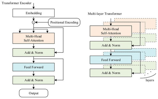
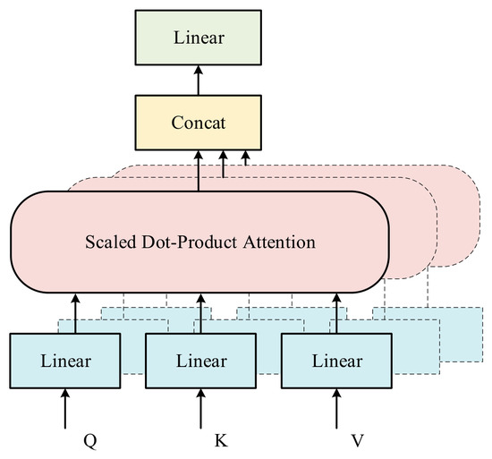
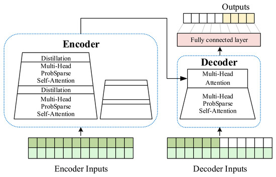
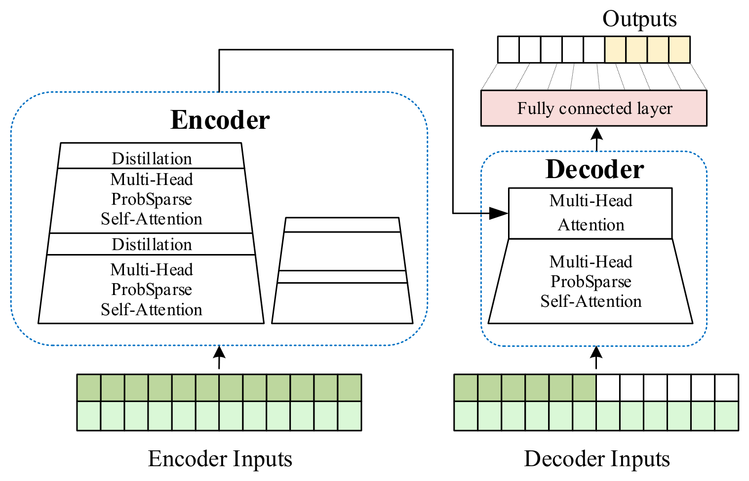
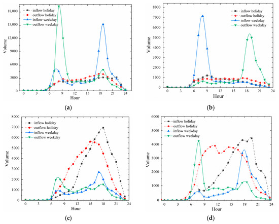
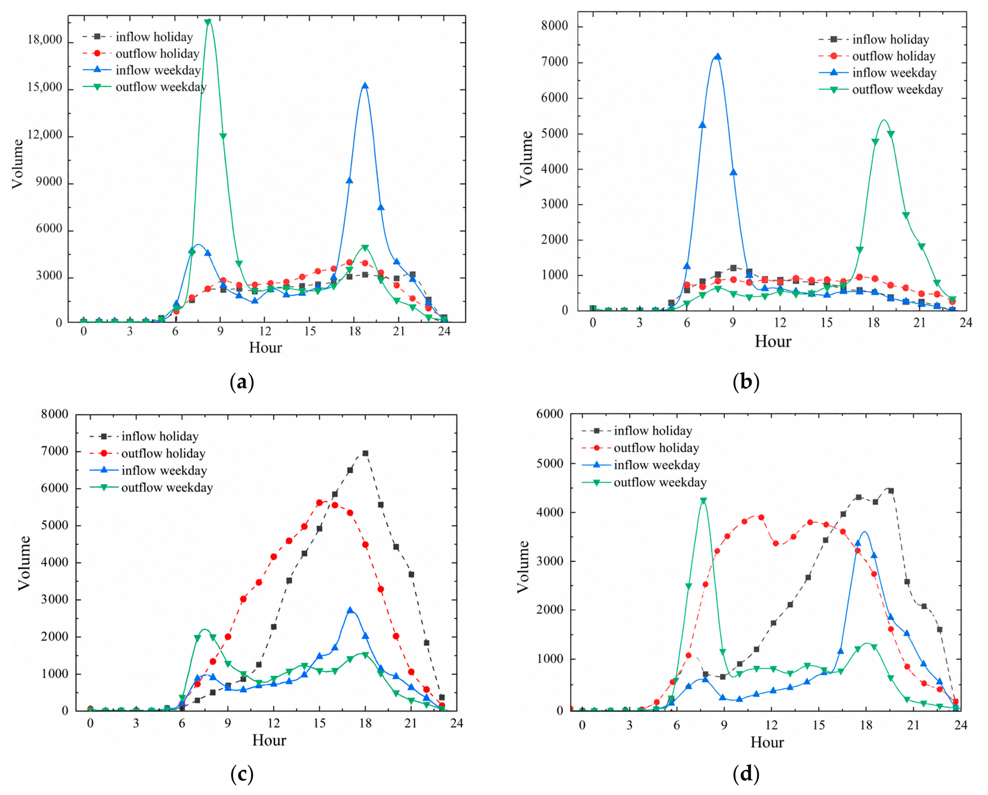
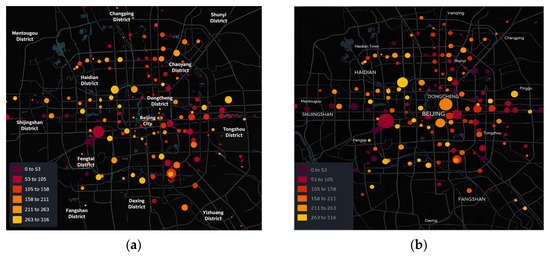
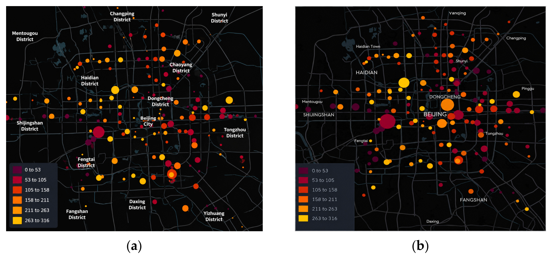
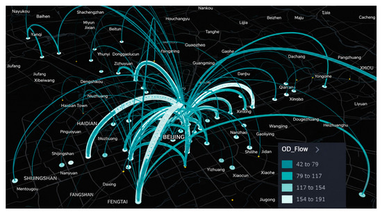
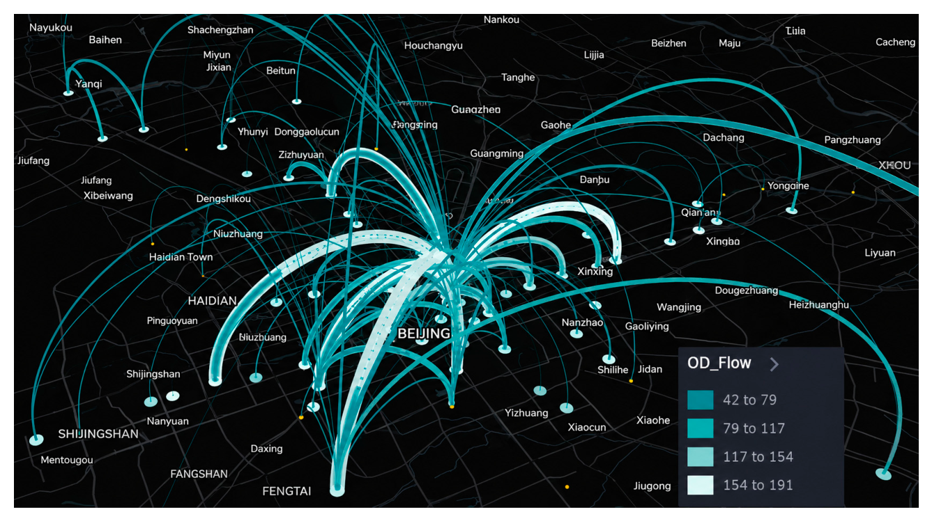
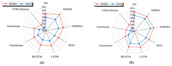

Disclaimer/Publisher’s Note: The statements, opinions and data contained in all publications are solely those of the individual author(s) and contributor(s) and not of MDPI and/or the editor(s). MDPI and/or the editor(s) disclaim responsibility for any injury to people or property resulting from any ideas, methods, instructions or products referred to in the content. |
© 2026 by the authors. Licensee MDPI, Basel, Switzerland. This article is an open access article distributed under the terms and conditions of the Creative Commons Attribution (CC BY) license.