A CNN–Mamba-Based Method for Visual Tire–Road Friction Potential Estimation Under Low-Excitation Variable Working Conditions

Abstract

The road surface adhesion coefficient is a key parameter affecting the dynamic control and driving safety of vehicles. Addressing the limitations of vehicle dynamics-based estimation methods under low-excitation conditions, this paper proposes a vision-perception-based CNN–Mamba hybrid regression network (CMHR-Net) for visual road friction potential estimation. By extracting road surface texture features from camera images, the proposed method predicts representative friction levels associated with different road conditions, providing prior information for vehicle active safety and control systems. First, ResNet18 is used to extract local texture features from road surface images. Second, a Mamba State Space Model is introduced to model long-distance dependencies between features, thereby enhancing global representation capabilities. Finally, the predicted adhesion coefficient value is output through a regression layer. Simultaneously, an adhesion coefficient mapping dataset based on road surface semantic attributes is constructed for model training and validation. Experimental results show that under various road surface conditions, including wet asphalt, waterlogged asphalt, waterlogged concrete, ice and snow, and joints, the proposed method significantly reduces the MAE (Mean Absolute Error) compared to the traditional CNN model. Specifically, under low adhesion conditions (μ ≈ 0.20), the error is reduced by approximately 56.9%. Furthermore, in complex variable conditions, the model significantly outperforms the traditional CNN model in both maximum error (Max Error) and mean absolute percentage error (MAPE). For example, under low adhesion conditions (μ ≈ 0.20), the MAPE decreases from 21.59% to 9.28%, and the maximum error decreases from 0.2025 to 0.0628, demonstrating superior stability and robustness. This method can achieve high-precision feedforward estimation of the adhesion coefficient without relying on vehicle dynamics excitation, providing effective support for feedforward control and active safety systems in vehicles.

1. Introduction

1.1. Research Background and Significance

The coefficient of adhesion (μ) is a core parameter describing the frictional characteristics between the tire and the road surface, and it has a decisive impact on the longitudinal dynamics and lateral stability of vehicles. In vehicles, the drive system uses an electric motor structure, which offers advantages such as fast response speed and high torque control precision. This allows the tire–road friction coefficient to directly participate in torque distribution, regenerative braking control, and the formulation of stability control strategies. Therefore, achieving high-precision, real-time acquisition of the tire–road friction coefficient is of great significance for improving the active safety performance of vehicles.

However, under low-excitation conditions such as low speed, constant speed, and small disturbances, tire slip information is insufficient, leading to reduced observability of estimation methods based on vehicle dynamics models. Simultaneously, in complex road environments, the road surface adhesion state exhibits significant spatial non-uniformity and dynamic variation characteristics, i.e., variable operating condition characteristics. These factors collectively make it difficult for traditional methods to achieve stable and reliable adhesion coefficient estimation.

With the development of deep learning technology, road perception methods based on visual information have gradually become a research hotspot. CNNs have significant advantages in image feature extraction, but their ability to model long-range dependencies is limited. In recent years, State Space Models (SSMs) have made significant progress in sequence modeling. Among them, the Mamba model, by introducing a selective state space mechanism, achieves efficient modeling of long-range dependencies while maintaining linear computational complexity, providing a new approach to global feature modeling in visual tasks.

Based on the above analysis, this paper proposes a CNN–Mamba hybrid regression network to address the problem of unreliable estimation of the adhesion coefficient under low-excitation conditions. By fusing the local feature extraction capabilities of CNNs with the global modeling capabilities of Mamba, continuous visual estimation of road friction levels is achieved. This method not only overcomes the shortcomings of traditional CNNs in long-range dependency modeling but also significantly improves the estimation accuracy and robustness of the model under low adhesion and complex variable working conditions, thus providing an effective approach for high-precision feedforward estimation of the adhesion coefficient.

It should be noted that the tire–road friction coefficient is jointly determined by road condition, tire characteristics, environmental factors, and vehicle operating states. Therefore, a vision-based method cannot directly measure the instantaneous tire–road friction coefficient. Instead, it provides an estimation of road friction potential based on observable surface characteristics.

The main contributions of this paper are as follows:

(1)

A CNN–Mamba hybrid architecture integrating convolutional neural networks and State Space Models is proposed to achieve continuous estimation of the road surface adhesion coefficient driven by visual information.

(2)

A continuous adhesion coefficient mapping modeling method based on road surface semantic attributes is proposed, which maps discrete road surface categories to physically meaningful continuous adhesion coefficient labels, realizing the transformation from road surface classification to adhesion coefficient regression.

1.2. Current Status of Research at Home and Abroad

Currently, scholars both domestically and internationally have conducted extensive research on the estimation of the road surface adhesion coefficient. Based on the different technical methods employed, these studies can be broadly categorized into three types: sensor-based methods, vehicle dynamics model-based methods, and data-driven methods.

1.2.1. Sensor-Based Adhesion Coefficient Estimation Method

The slip ratio curve estimation method estimates the relationship between tire slip ratio and road adhesion coefficient under different road conditions. Different road surfaces correspond to different slip slopes. Gustafsson et al. [1] proposed to estimate the slip slope using Kalman filtering and obtain the road adhesion coefficient through the relationship model between slip slope and adhesion coefficient. Rajamani et al. [2] used the recursive least squares method to estimate the slip slope to obtain the adhesion coefficient. Qi et al. [3] proposed an adhesion coefficient estimation method based on extended Kalman filtering, which also belongs to the slip ratio curve method. Yong et al. [4] identified the road surface type by establishing a typical road slip ratio curve and matching it with the current slip ratio curve, and then obtained the corresponding road adhesion coefficient by looking up a table.

This type of method has the advantage of high measurement accuracy, but its disadvantages are also quite obvious: high equipment cost, complex installation, and difficulty in large-scale deployment on ordinary vehicles. Therefore, this type of method is mainly used in road testing equipment or professional test vehicles, and its application in intelligent driving systems is somewhat limited.

1.2.2. Estimation Methods Based on Vehicle Dynamics Models

The vehicle dynamics model-based approach is currently one of the most widely studied methods. This method typically utilizes onboard signals such as wheel speed sensors, acceleration sensors, and steering wheel angle sensors, combined with vehicle dynamics models and tire models, to estimate the road surface adhesion coefficient using state estimation algorithms.

ZHANG et al. [5] proposed an improved Brush tire model and combined it with the square root commutative Kalman filter algorithm to estimate the road surface adhesion coefficient, which has high accuracy in longitudinal and lateral force estimation. CHEN et al. [6] used support vector machines to classify road texture features to achieve road surface type recognition; DU et al. [7] used a deep neural network based on domain knowledge to estimate the road surface adhesion coefficient. Gong et al. [8] calculated the normalized tire force based on the Unitire tire model and combined it with a commutative Kalman filter to estimate the adhesion coefficient. Hu et al. [9] introduced finite memory filtering and random weighting theory into unscented Kalman filtering to reduce the influence of measurement error; Wang et al. [10] proposed a fault-tolerant unscented Kalman filter algorithm to improve the estimation performance in the case of sensor data loss; Li et al. [11] improved the unscented Kalman filter by introducing a fading factor to improve the estimation accuracy. Lin et al. [12] combined unscented Kalman filtering with a two-dimensional LuGre model to achieve effective estimation of the road surface adhesion coefficient under straight and turning conditions.

However, this type of method is highly dependent on vehicle excitation. Under low-excitation conditions such as low speed or constant speed, the lack of sufficient tire slip information reduces system observability, leading to a significant decrease in estimation accuracy. Furthermore, model parameter uncertainties and tire model mismatch issues further affect the robustness of the estimation results.

1.2.3. Data-Driven Adhesion Coefficient Estimation Method

With the development of artificial intelligence technology, data-driven methods based on machine learning and deep learning have gradually become an important research direction for adhesion coefficient estimation. These methods establish data models to learn the relationship between the adhesion coefficient and input features from a large amount of historical or image data, thereby enabling the prediction of the adhesion coefficient.

Considering the above situation, Song S et al. [13] proposed a neural network system with added credibility, and randomly set the speed of the simulated vehicle and randomly input the operation of braking, steering and other changes in the vehicle’s motion state, and established a CNN-LSTM joint model. In such a large amount of training data, a method of prioritizing credibility was proposed, selectively selecting some training data. After processing, the network training was better, so the final estimation result was more accurate. The data used by the above neural networks all come from automotive dynamics software. In order to make the model more applicable to the environment, Fenyes et al. [14] proposed a method to estimate the friction coefficient by using big data and the friction force between the car tire and the road surface. In the selection of actual data, data is collected by sensors on the vehicle body such as gyroscopes and wheel speed sensors. The method uses real vehicle data. Finally, the C4.5 decision tree algorithm is used to classify different adhesion coefficients. The classification results are then matched with the results in the big data to obtain the adhesion coefficients of different road surfaces. Šabanovic et al. [15] designed a deep convolutional neural network and achieved an accuracy of 88.8% in identifying six types of road surfaces, including dry and wet asphalt, dry and wet cobblestones, and dry and wet gravel. Nolte et al. [16] compared the recognition performance of two deep convolutional neural networks, ResNet50 and InceptionNetV3, on six typical road surface datasets. The results showed that ResNet50 had a stronger classification ability than InceptionNetV3. Zhao et al. [17] proposed a vision-based real-time road friction estimation framework that combines a convolutional neural network (CNN) classification model with texture-aware feature extraction and stabilizing filters to achieve adhesion coefficient estimation under five friction categories. Research by Roychowdhury et al. [18] shows that a road friction factor estimation method based on a two-stage approach (CNN extracting road area features to classify road conditions and rule-based model segmenting to quantize drivable surfaces) is effective in autonomous driving scenarios. Zhao et al. [19] proposed a vision-based real-time road friction estimation framework that combines a convolutional neural network (CNN) classification model with texture-aware feature extraction and stabilizing filters.

Existing research often employs convolutional neural networks (CNNs) to extract features from road surface images, enabling road surface type identification or adhesion coefficient prediction. However, CNNs primarily rely on local receptive fields for feature extraction, making it difficult to effectively model long-distance spatial dependencies. This limits their ability to represent complex road surface structures (such as water film distribution and the continuity of snow and ice cover), resulting in insufficient prediction stability in complex environments.

In summary, existing methods for estimating the road adhesion coefficient mainly include sensor-based, vehicle dynamics model-based, and data-driven methods. Dynamics-based methods rely on excitation information such as tire slippage, which lacks observability under low-excitation conditions such as low speed or constant speed, leading to decreased estimation accuracy. While vision-based CNN methods possess the advantage of feedforward perception, they are limited by local receptive fields and lack the ability to model complex road surface spatial distributions and global structural features, affecting their stability under varying operating conditions. Therefore, improving the model’s ability to globally represent road adhesion characteristics under low-excitation conditions is a pressing issue that needs to be addressed.

Gu and Dao [20] proposed the Mamba architecture based on Selective State Space Models (SSMs), which enables efficient long-sequence modeling with linear computational complexity while preserving global contextual information. Owing to its superior balance between representation capability and computational efficiency, Mamba has attracted increasing attention in computer vision, time-series prediction, and intelligent transportation applications. Motivated by these advantages, this study integrates a Mamba module into a CNN-based framework to enhance global feature extraction and improve the robustness of visual friction potential estimation under varying road conditions.

Based on this, this paper proposes a CNN–Mamba hybrid regression network, which integrates the local feature extraction capability of convolutional neural networks with the global modeling capability of Mamba models to achieve high-precision continuous prediction of the road surface adhesion coefficient.

The remainder of this paper is organized as follows:

Section 2 introduces the construction of the road surface dataset and the assignment strategy of visual friction potential labels.

Section 3 presents the proposed CNN–Mamba network architecture and its implementation details.

Section 4 describes the experimental setup and evaluates the performance of the proposed method under various road conditions. Furthermore, a closed-loop vehicle dynamics validation based on a seven-degree-of-freedom vehicle model and the tire model is conducted to assess the practical applicability of the predicted friction information.

Finally, Section 5 summarizes the main conclusions and discusses future research directions.

2. Road Surface Adhesion Coefficient Label Construction and Mapping Method

2.1. Dataset and Road Surface Type Classification

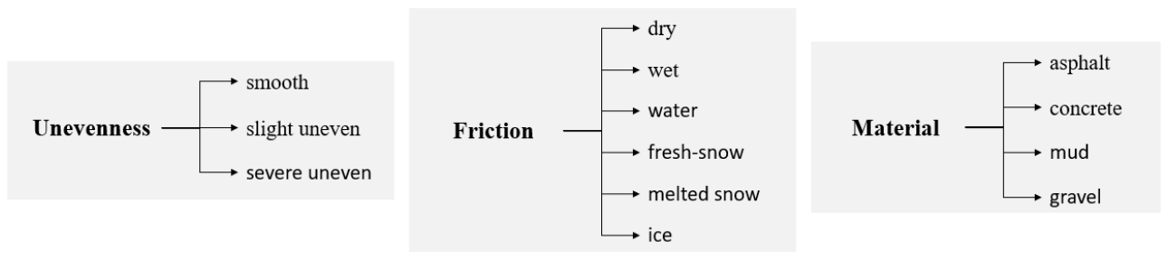
To train the road surface adhesion coefficient prediction model, this paper uses the open-source RSCD [20] dataset. The three road attribute subclasses are combined to form the category definition of the dataset, with a total of 27 types, as shown in Figure 1.

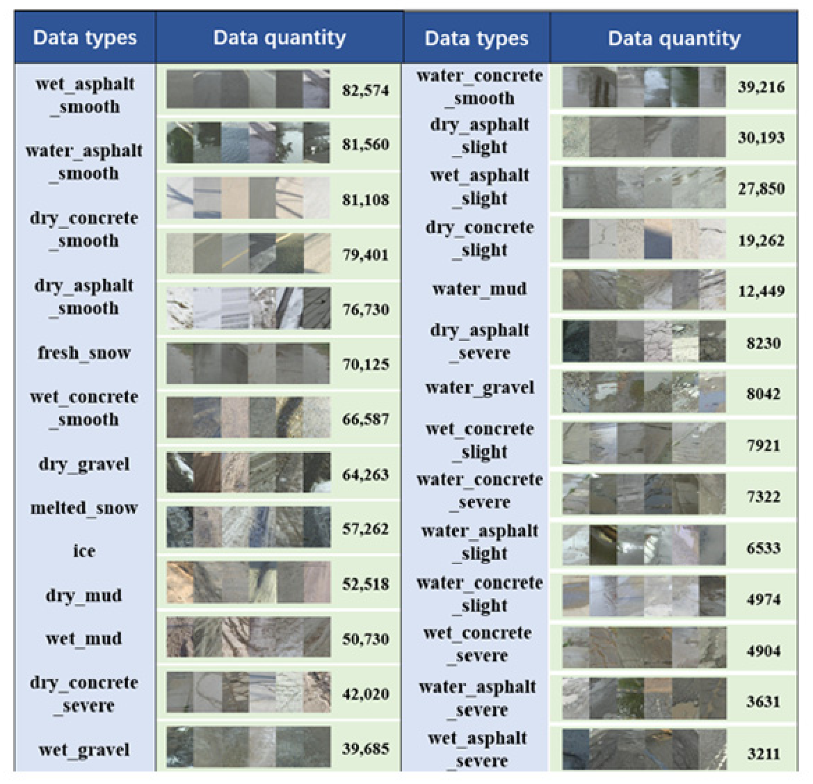
The dataset is shown in Figure 2 below:

2.2. Adhesion Coefficient Label Setting and Mapping Rules

Since publicly available road image datasets typically do not provide accurate measurements of pavement adhesion coefficients, this paper employs an empirical adhesion coefficient mapping method based on pavement type to construct supervised learning labels. This method maps different pavement categories to corresponding adhesion coefficient values based on typical friction coefficient ranges provided in road engineering and vehicle dynamics studies.

Studies have shown that different road surface materials and moisture conditions have a significant influence on tire–road friction characteristics. Based on representative friction ranges reported in road engineering, terramechanics, and vehicle dynamics studies:

The tire–road friction coefficient on dry asphalt pavement is typically between 0.8 and 0.9;

The tire–road friction coefficient on wet asphalt pavement is generally between 0.5 and 0.6;

The tire–road friction coefficient on snow-covered surfaces is approximately 0.2–0.3;

The tire–road friction coefficient on icy surfaces is usually lower than 0.1–0.15.

Based on these representative friction ranges, a visual friction potential mapping strategy is established to construct the training labels used in this study.

The friction ranges adopted in this study were determined based on typical tire–road friction values reported in References [21,22,23,24,25,26]. Previous studies have shown that the tire–road friction coefficient is not a fixed value, but varies with tire type, tread wear, tire pressure, temperature, road surface texture, water film thickness and vehicle operating conditions. Therefore, for each road surface type, friction ranges were used rather than fixed values. The mean values reported in

Table 1. Friction coefficient labels for different road surface types.

Road Surface Type	Typical Friction Range	Representative Value	Road Surface Type	Typical Friction Range	Representative Value
dry_asphalt_smooth	0.85–0.95	0.90	wet_gravel	0.25–0.45	0.35
dry_asphalt_slight	0.75–0.85	0.80	wet_mud	0.15–0.30	0.25
dry_asphalt_severe	0.70–0.80	0.75	water_asphalt_smooth	0.40–0.60	0.50
dry_concrete_smooth	0.80–0.90	0.85	water_asphalt_slight	0.35–0.55	0.45
dry_concrete_slight	0.70–0.85	0.78	water_asphalt_severe	0.30–0.50	0.40
dry_concrete_severe	0.65–0.80	0.72	water_concrete_smooth	0.38–0.58	0.48
dry_gravel	0.35–0.50	0.40	water_concrete_slight	0.35–0.55	0.45
dry_mud	0.20–0.35	0.30	water_concrete_severe	0.28–0.48	0.38
wet_asphalt_smooth	0.50–0.70	0.60	water_gravel	0.25–0.45	0.35
wet_asphalt_slight	0.45–0.65	0.55	water_mud	0.10–0.30	0.22
wet_asphalt_severe	0.40–0.60	0.50	fresh_snow	0.15–0.35	0.25
wet_concrete_smooth	0.50–0.65	0.58	melted_snow	0.10–0.30	0.20
wet_concrete_slight	0.45–0.60	0.53	ice	0.05–0.15	0.10
wet_concrete_severe	0.40–0.55	0.48

were selected as the midpoints of the intervals, whilst the upper and lower limits were determined based on the ranges commonly reported in the literature. This approach is consistent with recent visual-based studies on friction coefficient estimation and better reflects the uncertainty inherent in actual tire–road interactions.

It should be noted that the tire–road friction coefficient is not a deterministic constant for a given road category. The actual friction level is affected by tire type, tread wear, inflation pressure, temperature, vehicle speed, road contamination, and water-film thickness. Therefore, Table 1 provides typical friction ranges collected from the vehicle dynamics and terramechanics literature. For supervised learning, the representative value of each range was adopted as the training label.

In the data annotation process, this paper assigns a corresponding adhesion coefficient label to each image based on the road surface type, thereby constructing a supervised learning dataset. All images are uniformly adjusted to 224 × 224 and undergo data augmentation processing, including random flipping, brightness perturbation, and contrast adjustment, to improve the model’s generalization ability.

2.3. Discussion of Friction Labels

It should be noted that the friction labels used in this study are derived from representative friction coefficient values associated with different road surface categories, as reported in the literature. Consequently, these labels do not represent the precise instantaneous friction coefficient for each individual image.

In reality, road surface friction is influenced by a variety of factors, including road surface wear, temperature, contaminants and the thickness of the water film. Therefore, the actual friction coefficients of different images belonging to the same road category may vary.

Due to the lack of image-specific friction measurement data in publicly available RSCD datasets, this study is unable to explicitly model these variations. Consequently, the proposed method should be regarded as a vision-based framework for estimating road friction, designed to predict representative friction levels associated with observed road conditions, rather than directly measuring the true physical coefficient of friction.

Future work will focus on integrating on-board sensor measurements, tire–road interaction data, and field test results to establish image-level friction labels and further improve the physical accuracy of friction estimates.

3. CNN–Mamba Hybrid Regression Network

3.1. Overall Network Structure

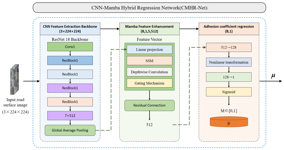
To achieve continuous prediction of the road surface adhesion coefficient based on visual information, this paper proposes a CNN–Mamba Hybrid Regression Network (CMHR-Net). This network takes a road surface image as input, extracts road surface texture features through a convolutional neural network, and introduces a Mamba module to perform nonlinear enhancement modeling of high-level features. Finally, it outputs continuous predicted values of the road surface adhesion coefficient through a regression head.

The proposed CNN–Mamba hybrid regression network structure is shown in Figure 3, and mainly consists of the following three parts:

(1)

CNN feature extraction module: used to extract local texture features of the road surface;

(2)

Mamba Feature Enhancement Module: used for dynamic modeling and nonlinear representation enhancement of high-dimensional features;

(3)

Regression Prediction Module: outputs predicted values of road surface adhesion coefficient.

The mathematical form can be expressed as:

$$\mu =f_{reg}(f_{mamba}(f_{cnn}(X)))$$

(1)

In the formula: $X$ is the input road surface image, $f_{cnn}(·)$ represents the CNN feature extraction process; $f_{\mathit{mamba}}(·)$ is the Mamba feature enhancement module; $f_{\mathit{reg}}(·)$ represents the regression prediction module; $\mu$ represents the predicted road adhesion coefficient.

3.2. CNN Feature Extraction Module

In the visual adhesion coefficient estimation task, road surface texture features (such as particle roughness, water film reflection features, and snow and ice cover features) are closely related to tire–road friction characteristics. Therefore, convolutional neural networks are needed to effectively extract features from images.

This paper uses ResNet18 as the basic feature extraction network. ResNet solves the gradient vanishing problem during the training of deep networks through a residual connection structure and can effectively extract multi-scale texture information.

The basic residual structure of ResNet can be represented as:

$$y=F(x,W)+x$$

(2)

In the formula: $x$ is the input feature; $F(x,W)$ represents the convolution transformation; $y$ represents the output feature.

Residual connections enable the network to learn residual mappings, thereby improving training stability.

In this paper, the ResNet18 network structure retains its convolutional layer structure, removing only the last fully connected layer to extract high-level semantic features of the image. After feature extraction, a 512-dimensional feature vector is obtained:

$$F_{cnn}\in {ℝ}^{B\times 512}$$

(3)

The feature vector is then fed into the Mamba feature enhancement module for further processing.

3.3. Mamba Enhancement Module

To address the shortcomings of traditional CNNs in long-range dependency modeling, this paper introduces the Mamba module to enhance the modeling of high-dimensional features. Mamba is an efficient sequence modeling method based on the Selective State Space Model (SSM), which can capture long-range dependencies while maintaining low computational complexity.

Unlike typical sequence tasks, this paper reconstructs the feature vectors extracted by CNN into a one-dimensional feature sequence, thereby introducing sequence modeling capabilities in the spatial dimension, enabling the model to capture macroscopic structural information in road images.

The module mainly includes the following structures: Linear Projection, Selective State Space Model (SSM), Depthwise Convolution, Gating Mechanism, and Residual Connection.

First, the input features are mapped using linear projection to enhance their expressive power:

$$F^{\prime }=W{F}_{cnn}$$

(4)

In the formula: $W$ is a learnable parameter.

Subsequently, a selective State Space Model is used to dynamically model the feature sequence. Its state update process can be represented as:

$$h_t=A_t{h}_{t-1}+B_t{x}_t$$

(5)

The output is:

$$y_t=C_t{h}_t$$

(6)

In the formula: $h_t$ represents the hidden state; $x_t$ represents the input features; and $A_t$, $B_t$, and $C_t$ are the model parameters.

Furthermore, depthwise convolution is introduced after state space computation to capture local feature information, thereby enhancing the model’s ability to express spatial structural features.

To control information flow and improve model stability, a gating mechanism (Gate) is also designed into the module. The gating function has the following form:

$$G=\sigma (W_{g}x)$$

(7)

The final output is achieved through gated fusion:

$$H=G\cdot Z+(1-G)\cdot X$$

(8)

In the formula: $Z$ represents the output of the Mamba module; $X$ represents the input characteristics.

Finally, the input features and the enhanced features are fused through residual connections:

$$F_{out}=X+H$$

(9)

This structure can effectively avoid the gradient vanishing problem that occurs during the training of deep networks.

Enhanced features are obtained after processing with the Mamba module:

$$F_{mamba}\in {ℝ}^{B\times 512}$$

(10)

3.3.1. Feature Sequence Construction

After feature extraction, the output of ResNet18 is a feature vector with dimension 512:

$$z=[z_1,z_2,\dots ,z_{512}]$$

(11)

Unlike conventional image classification tasks, the extracted feature vector is regarded as a one-dimensional feature sequence and directly fed into the Mamba module.

Specifically, the feature vector is reshaped as:

$$z=[z_1,z_2,\dots ,z_n]$$

(12)

where n = 512 denotes the sequence length.

By converting the CNN feature representation into a sequential form, the Mamba module can model long-range dependencies among different feature channels and capture global structural information embedded in the road image.

3.3.2. End-to-End Training Strategy

The proposed CNN–Mamba network is trained in an end-to-end manner.

During training, the parameters of the CNN feature extractor, Mamba enhancement module, and regression head are optimized simultaneously using backpropagation.

Given the predicted road friction coefficient $\widehat{\mathrm{\mu }}$ and ground-truth label μ, the mean squared error loss is defined.

Where N denotes the batch size.

The gradients are propagated from the regression layer to the Mamba module and further to the CNN feature extractor, allowing all network parameters to be jointly optimized.

3.4. Road Surface Adhesion Coefficient Regression Module

After obtaining the enhanced features, the network enters the regression prediction stage. The regression module consists of two fully connected layers, with the following structure:

First, the feature dimension is reduced from 512 to 128 using the first fully connected layer:

$$F_1=W_1{F}_{mamba}$$

(13)

Then, nonlinearity is introduced through the ReLU activation function:

$$F_2=\max (0,F_1)$$

(14)

Finally, the predicted value is obtained through the second fully connected layer:

$$\widehat{\mu }=W_2{F}_2$$

(15)

Since the physical range of the road surface adhesion coefficient is: $\mu \in [0,1]$, the Sigmoid function is used for normalization in the output layer:

$$\mu ={\displaystyle \frac{1}{1+e^{-x}}}$$

(16)

The final output is the predicted road surface adhesion coefficient.

4. Experimental Design and Results Analysis

4.1. Experimental Platform and Implementation Environment

The experiments in this paper were completed in the VSCode (Visual Studio Code 1.123.2) development environment, with Python as the main development language, and the training and testing of the CNN–Mamba network model were implemented using the deep learning framework PyTorch3.10.19.

The hardware and software environment of the experimental platform is shown in

Table 2. Experimental platform information.

Type	Configuration
Operating system	Ubuntu
Development framework	PyTorch
Programming language	Python 3.10
GPU	NVIDIA GeForce RTX 2060
CUDA	13.1

below:

4.2. Dataset Construction and Preprocessing

Based on the above dataset, different road conditions correspond to different adhesion coefficients, and the dataset is divided according to the proportion of 85% training set and 15% verification set.

In order to improve the generalization ability of the model, the data is preprocessed before training: including image size uniformity; data normalization; data enhancement (flip, rotate, brightness perturbation).

4.3. Model Training

The main training parameters are as follows in

Table 3. Training parameters.

Parameter	Numerical Values
Batch Size	16
Learning rate	1 × 10−4
Optimizer	Adam
Loss function	MSELoss
Training/Validation Ratio	85%/15%

:

To verify the effectiveness of the proposed method, this paper sets up a comparison between a CNN regression model (ResNet18) and a CNN–Mamba regression model (the method described in this paper). The model performance is evaluated by comparing the prediction error and inference speed.

Backbone Network Comparison

To validate the suitability of ResNet18 as a backbone network for feature extraction, this paper further compares the predictive performance of attachment coefficients when using convolutional neural networks of varying complexity as feature extractors. The experiments selected the lightweight MobileNetV3, the ResNet18 used in this paper, and the deeper ResNet50 as comparison models.

To ensure experimental fairness, all networks employed the same dataset partitioning, training parameters and overall CNN–Mamba architecture, with only the CNN feature extraction module being replaced. Training parameters were kept consistent, including a batch size of 16, a learning rate of 1 × 10⁻⁴, the Adam optimizer and the MSELoss loss function.

The experimental results are are as follows in

Table 4. Training parameters.

Backbone	Params (M)	MAE	RMSE
MobileNetV3	5.4	0.024	0.031
ResNet18	11.7	0.018	0.023
ResNet50	25.6	0.015	0.020

:

The experimental results show that, although MobileNetV3 has fewer parameters and lower computational overhead, its limited network capacity results in a relatively weak ability to extract complex road surface texture features, leading to significant prediction errors.

In contrast, ResNet50 has a deeper network architecture and stronger feature representation capabilities, and its prediction accuracy is slightly better than that of ResNet18. However, ResNet50 has approximately more than twice the number of parameters of ResNet18, resulting in significantly increased computational complexity, which would impose a greater computational burden in real-time in-vehicle application scenarios.

Based on a comprehensive analysis of prediction accuracy and computational efficiency, ResNet18 offers lower computational complexity whilst ensuring high prediction performance, thereby achieving a good balance between accuracy and real-time performance. Based on the above considerations, this paper ultimately selects ResNet18 as the backbone feature extractor for the CNN–Mamba network.

Furthermore, it should be noted that the focus of this study lies in verifying the role of the Mamba module in enhancing the prediction performance of the adhesion coefficient, rather than designing a new convolutional feature extraction network. Therefore, adopting ResNet18—which features a mature architecture, is widely used, and offers stable performance—as the base feature extractor allows for a more objective evaluation of the effectiveness of the proposed method.

4.4. Experimental Results Analysis

Experimental comparisons were conducted under various typical road surface conditions. The advantages of the proposed method in terms of estimation accuracy, stability, and real-time performance were further verified through quantitative evaluation and performance analysis of the model’s estimation results.

4.4.1. Estimation Results Under Different Road Surface Conditions

In the experiment, several typical road surface types were selected, including wet asphalt pavement, waterlogged asphalt pavement, waterlogged concrete pavement, icy and snowy pavement, and connecting pavement, to simulate vehicle driving conditions in complex environments. By inputting the corresponding road surface, the road adhesion coefficient was predicted using both the ResNet18 regression model and the CNN–Mamba regression model. The predicted results were then compared with the reference friction labels, as shown below.

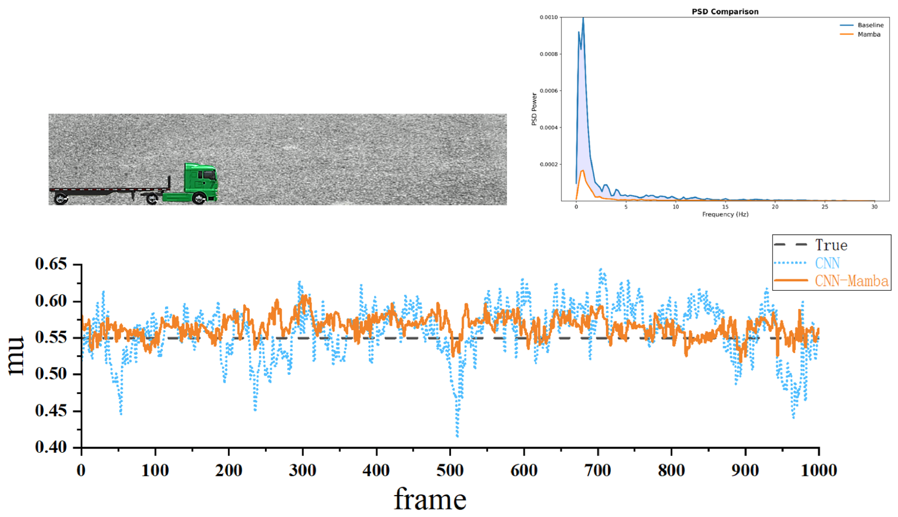
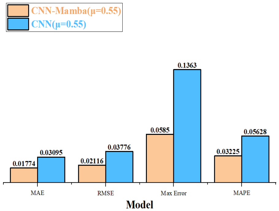
The results of a slightly uneven wet asphalt pavement (0.55) are shown in Figure 4 below:

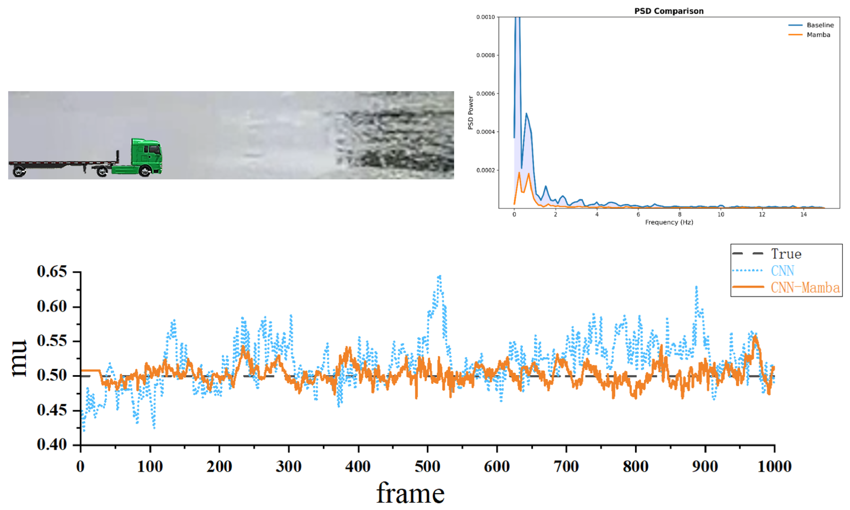
The result of intact asphalt pavement with water accumulation (0.50) is shown in Figure 5 below:

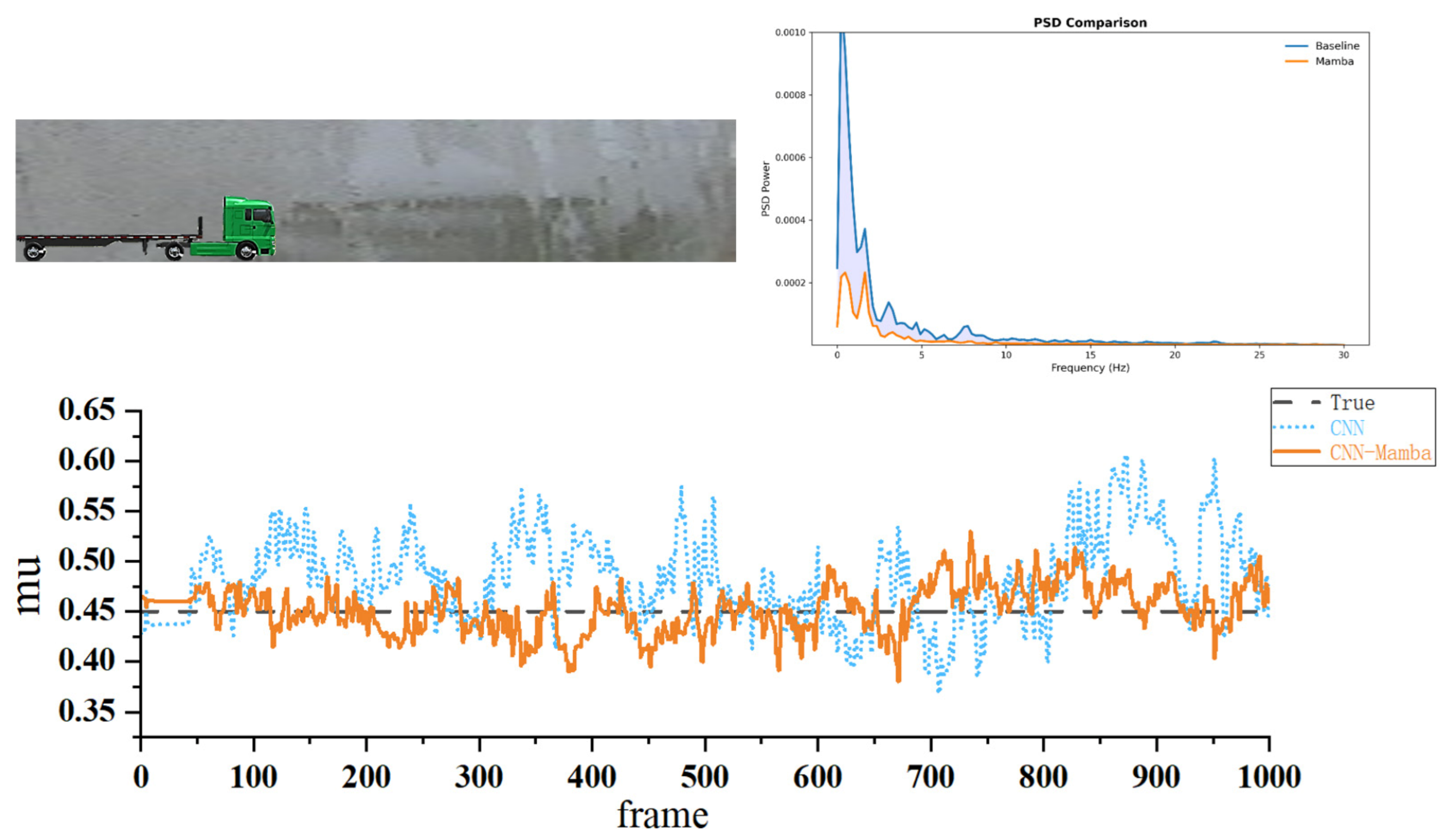
The results of a slightly uneven concrete pavement with water accumulation (0.45) are shown in Figure 6 below:

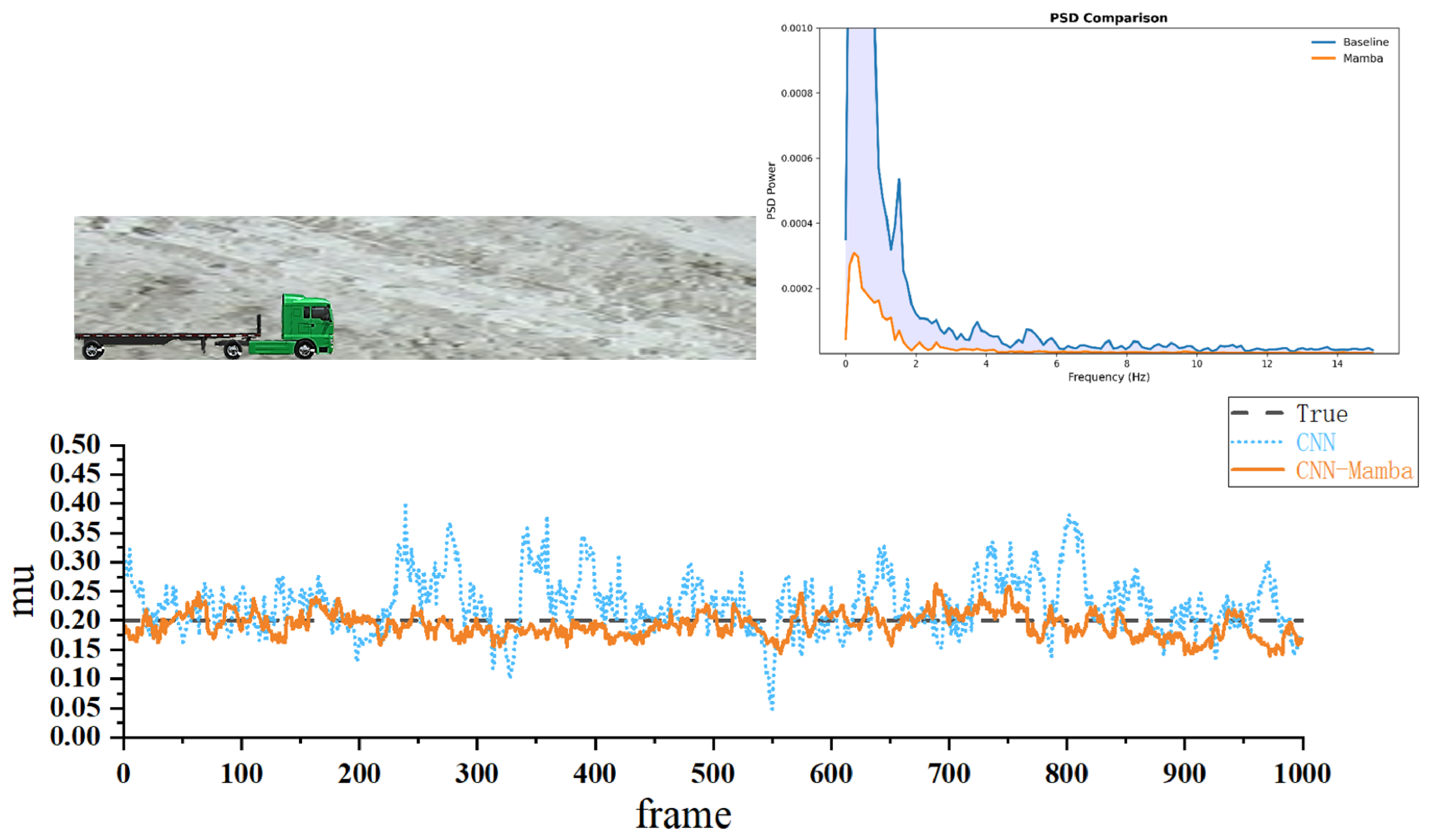
The results for icy and snowy road surfaces (0.20) are shown in Figure 7 below:

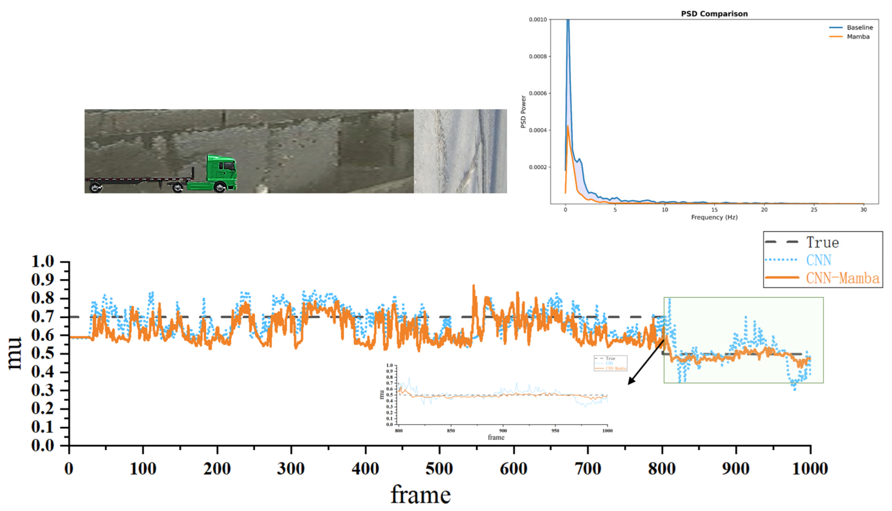
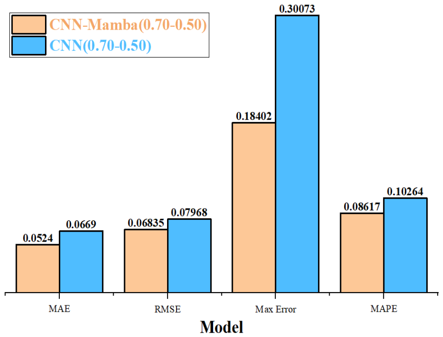
The transition in Figure 8 was modeled as a step change by concatenating two video sequences with μ = 0.70 and μ = 0.50. This setup evaluates the model’s response to abrupt road condition changes. The result of the connection to the road surface (0.70-0.50) is shown in Figure 8 below:

4.4.2. Real-Time Performance Evaluation

To evaluate the real-time applicability of the proposed method, the inference latency and effective frame rate (FPS) were measured on the experimental platform described in Table 2. Each frame’s forward propagation time through the network (i.e., from inputting a single road image to obtaining the estimated friction) was recorded and averaged over the testing sequences.

The results are summarized in

Table 5. Real-time performance comparison.

Model	Inference Time (ms/Frame)	FPS
CNN	4.6	217
CNN–Mamba	5.5	182

Note: Inference time is measured from the input of a single road image to the network output. FPS is calculated as the reciprocal of the average inference time.

. The conventional CNN baseline model achieves an average inference latency of 4.6 ms per frame (≈217 FPS), while the proposed CNN–Mamba framework introduces a slight computational overhead due to the additional Mamba module, resulting in an average latency of 5.5 ms per frame (≈182 FPS). Although Mamba is slightly slower than the baseline, both models far exceed typical onboard camera frame rates (25–30 FPS) and therefore satisfy real-time requirements for vehicle perception systems.

To address practical deployment, we estimated how far a vehicle would travel during a single inference cycle. Assuming a vehicle speed of 60 km/h (16.67 m/s), the corresponding traveling distance for one CNN–Mamba inference is approximately 0.092 m. This confirms that the estimated friction information can be obtained sufficiently early to be used by onboard vehicle controllers for braking, traction control, and stability management.

In addition to real-time feasibility, the CNN–Mamba framework significantly improves prediction quality compared with the baseline. Mamba achieves lower prediction variance (standard deviation 0.0329 vs. 0.0563) and higher temporal stability (smoothness 0.0130 vs. 0.0291). Therefore, although inference is slightly slower, the output is considerably more accurate and stable, which is critical for vehicle control applications.

4.4.3. Analysis of Estimation Results

This paper analyzes the experimental results from the aspects of prediction accuracy and model stability, and compares the proposed CNN–Mamba model with the traditional CNN regression model (ResNet18). The specific results are shown in

Table 6. Results analysis.

Model	MAE	RMSE	Max Error	MAPE (%)
CNN (μ = 0.20)	0.043173516	0.057143395	0.20251	21.58675824
CNN–Mamba (μ = 0.20)	0.01855006	0.02263569	0.06277	9.27502997
CNN (μ = 0.45)	0.043044705	0.05470047	0.15679	9.565490065
CNN–Mamba (μ = 0.45)	0.01931029	0.024076766	0.07975	4.291175491
CNN (μ = 0.50)	0.030870899	0.039977195	0.14547	6.17417982
CNN–Mamba (μ = 0.50)	0.010733107	0.01394308	0.05829	2.146621379
CNN (μ = 0.55)	0.030954685	0.037760034	0.1363	5.628124603
CNN–Mamba (μ = 0.55)	0.017736224	0.021156018	0.0585	3.224767959
CNN (μ = 0.70-0.55)	0.066901898	0.079682265	0.30073	10.26393321
CNN–Mamba (μ = 0.70-0.50)	0.052402577	0.068350013	0.18402	8.61668903

below:

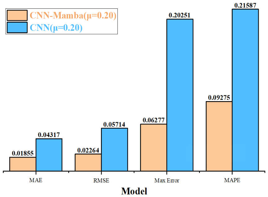
As shown in Figure 9, under the condition of low adhesion of ice and snow, the MAE of the CNN model is 0.0432, while that of the CNN–Mamba model is reduced to 0.0186, with the error decreasing by about 57%.

In this scenario, the road surface texture is extremely uniform, and the image exhibits large areas of low contrast. Traditional CNNs, relying on local textures for feature extraction, struggle to effectively distinguish between ice and snow and other light-colored road surfaces, resulting in significant estimation errors. In contrast, the CNN–Mamba model, through its state space modeling mechanism, can capture the overall brightness distribution and spatial consistency of the image, enhancing feature representation capabilities at a global level.

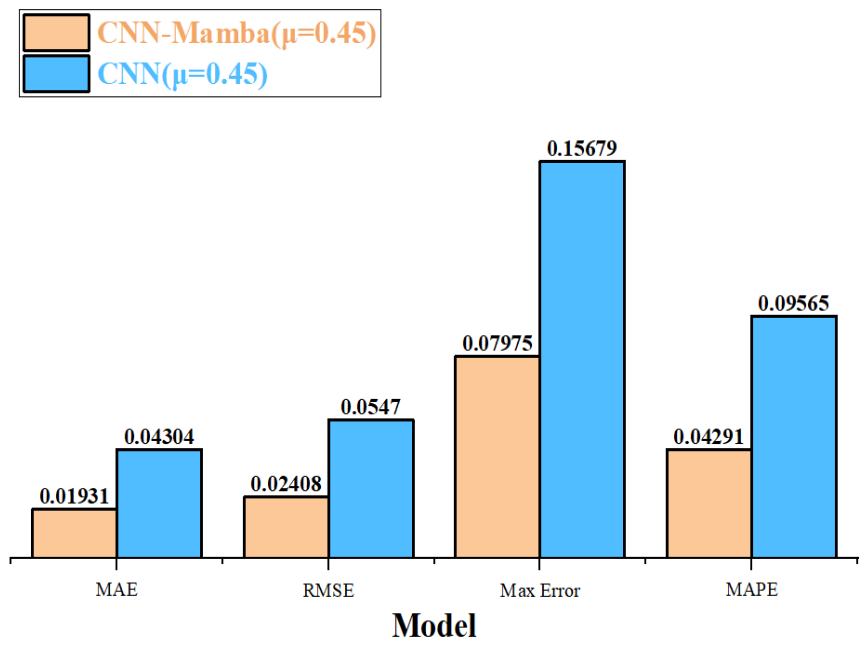
As shown in Figure 10, under the condition of slightly uneven concrete pavement with water accumulation, the MAE of the CNN model is 0.0430, while that of the CNN–Mamba model is 0.0193, with the error reduced by about 55%.

Under this condition, the road surface exhibits an uneven water film distribution, resulting in enhanced local reflection but partially weakened texture information. CNN models primarily rely on local brightness variations for judgment, making them susceptible to local noise interference. In contrast, the CNN–Mamba model can capture the spatial continuity of the water film distribution through global modeling, thereby obtaining more stable prediction results.

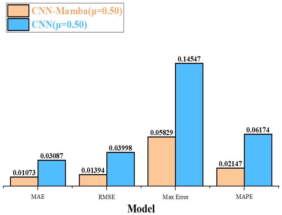
As shown in Figure 11, under the condition of intact asphalt pavement with water accumulation, the MAE of the CNN model is 0.0309, while that of the CNN–Mamba model is reduced to 0.0107, with an error reduction of about 65%, which is the largest reduction among all working conditions.

In this condition, the road surface is covered by a continuous film of water, exhibiting obvious specular reflection characteristics, with local textures almost disappearing. CNN models are prone to misjudging due to highlight areas, while the CNN–Mamba model, by modeling global reflectivity, can accurately identify the degree of water film coverage, thus achieving a more accurate estimation of the adhesion coefficient.

As shown in Figure 12, under the condition of slightly uneven and wet asphalt pavement, the MAE of the CNN model is 0.0310, while that of the CNN–Mamba model is 0.0177, with the error reduced by about 43%.

Under these conditions, the road surface exhibits both textured features and slight slipperiness, classifying it as a moderately complex adhesion scenario. While CNN models can extract texture information, they are insensitive to changes in slipperiness; whereas the CNN–Mamba model, by fusing local and global information, achieves a more refined depiction of adhesion variations.

As shown in Figure 13, under the condition of connecting road surface (non-uniform adhesion), the MAE of the CNN model is 0.0669, and that of the CNN–Mamba model is 0.0524, with the error reduced by about 21%.

This operating condition exhibits regions with significant abrupt changes in the adhesion coefficient, representing a typical variable operating scenario. CNN models, due to their limited receptive field, struggle to accurately identify these region boundaries, easily leading to averaging errors. In contrast, the CNN–Mamba model, by modeling cross-regional dependencies, can identify regions of abrupt adhesion changes, thereby improving prediction accuracy.

In summary, the data results show that the CNN–Mamba model outperforms the traditional CNN model under all typical low-excitation and variable working conditions. In particular, it exhibits significant accuracy improvement and stronger robustness in low-attachment and complex spatial distribution scenarios, verifying the application potential of the proposed method in real-world complex road environments.

4.5. Closed-Loop Vehicle Dynamics Validation

To further evaluate the engineering applicability of the proposed visual friction estimation method, a seven-degree-of-freedom vehicle dynamics model was established in MATLAB(R2024a)/Simulink. The model includes longitudinal, lateral, and yaw motions of the vehicle body, together with the rotational dynamics of four wheels. A tire model was employed to characterize tire–road interactions.

The friction coefficient sequence predicted by the CNN–Mamba network was imported into the vehicle model as feedforward road information and used to update the tire–road friction condition during simulation. For comparison, simulations using a constant friction coefficient (mu = 0.45) were also performed under the same driving conditions.

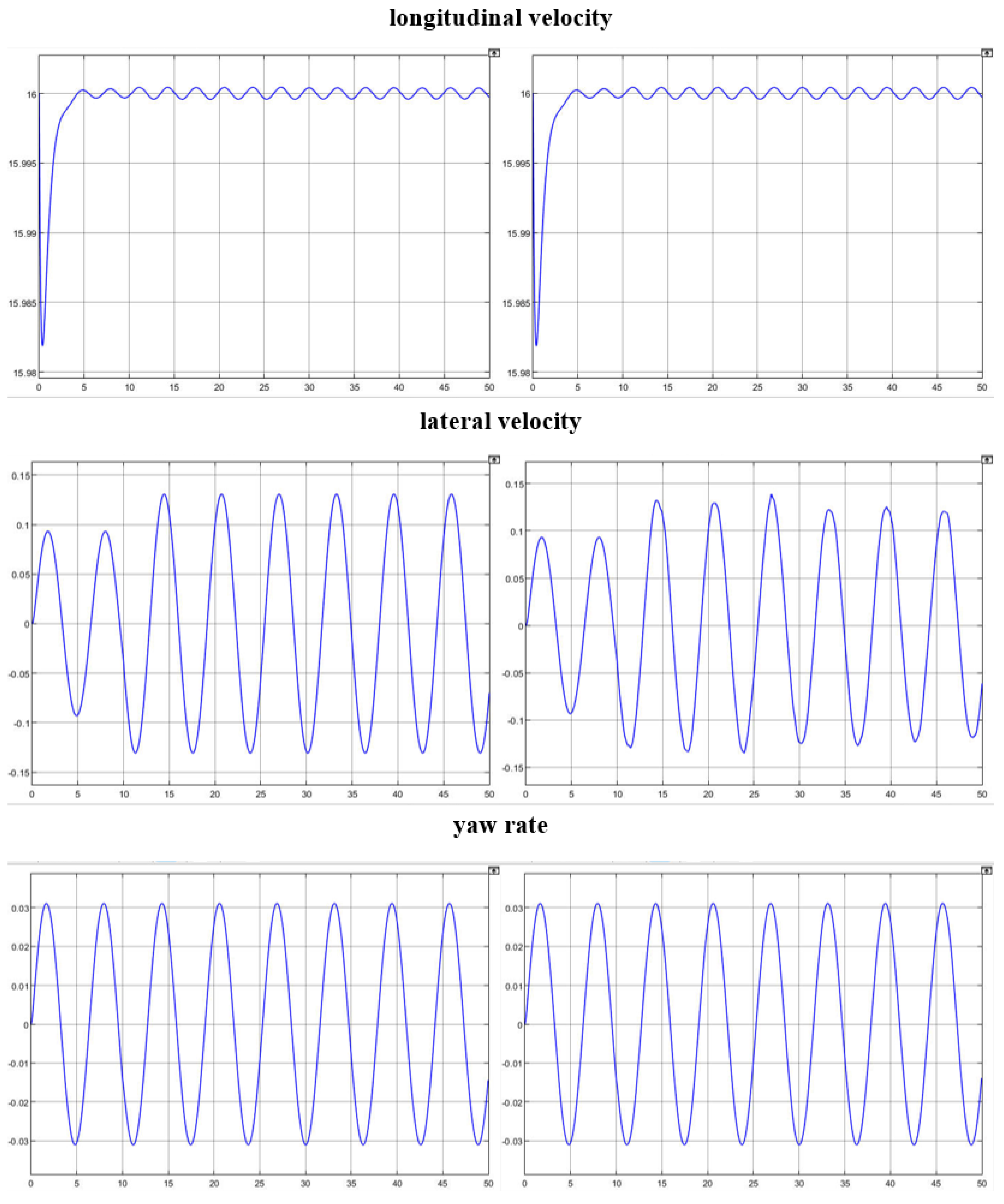
The simulation results indicate that the longitudinal velocity, lateral velocity, and yaw rate obtained using the predicted friction coefficient are highly consistent with those obtained using the constant friction coefficient.

The results demonstrate that the proposed CNN–Mamba model can provide stable and physically reasonable visual friction estimates, which can be directly utilized as feedforward information for vehicle dynamics control systems. The simulated results are shown in Figure 14:

At the same time, braking distances were evaluated under different friction estimation methods, whilst the coefficient of friction varied (μ: 0.7-0.5).

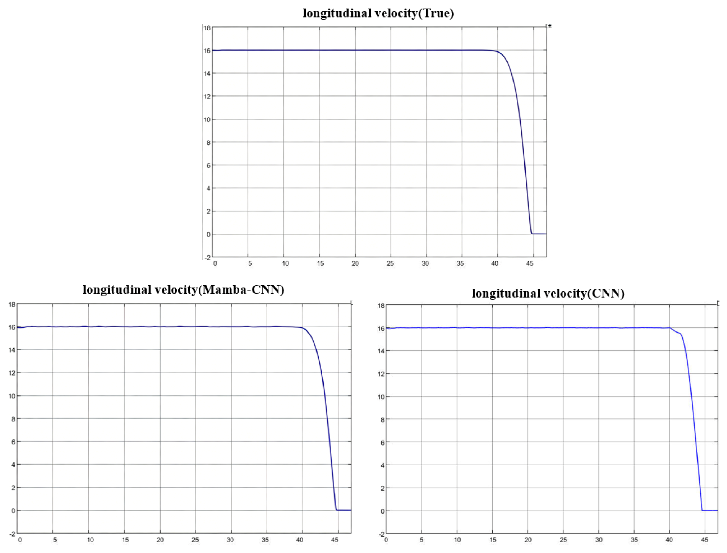
The longitudinal velocity response of the vehicle is shown under different friction estimation methods. The vehicle initially travels at 16 m/s, and braking is activated at 25 s while the road adhesion coefficient varies between 0.7 and 0.5.

After braking is applied, the velocity exhibits a monotonic decreasing trend with a nonlinear deceleration profile. The reduction in velocity is rapid in the initial braking phase and gradually slows down as the vehicle approaches a standstill, which is consistent with the nonlinear characteristics of tire–road interaction.

Compared with the CNN-based estimator, the proposed Mamba-based method produces a smoother velocity trajectory with reduced fluctuations, indicating improved stability of the closed-loop vehicle system. The results demonstrate that more accurate friction estimation contributes to more physically consistent vehicle deceleration behavior. The results of the experiment are shown in Figure 15.

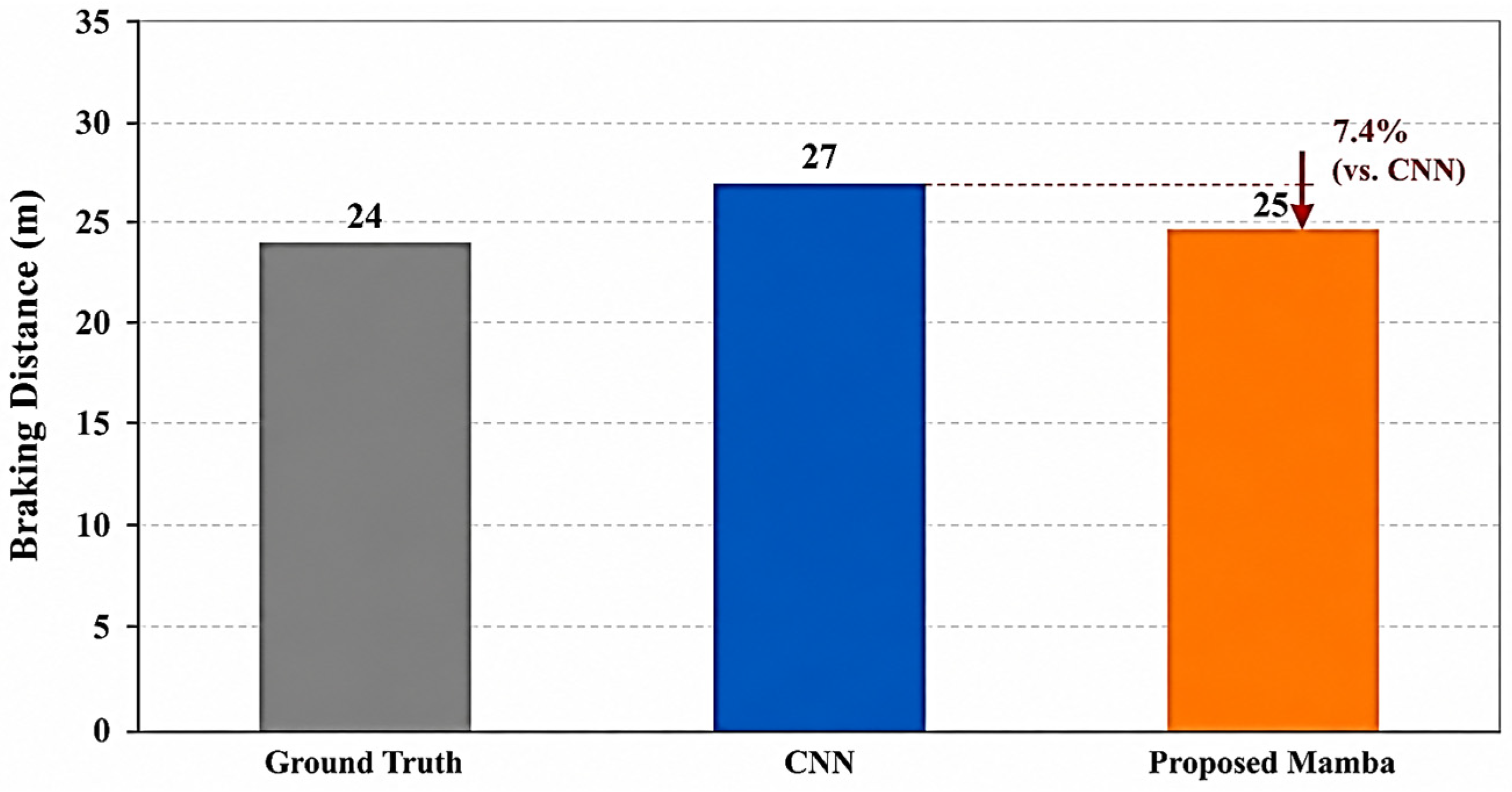
The results show that the CNN-based method yields the largest braking distance (27 m), indicating over/under-estimation of road friction, while the proposed Mamba-based method (25 m) closely matches the ground truth case (24 m), demonstrating improved estimation accuracy and better closed-loop control performance. The results of the experiment are shown in Figure 16.

The proposed Mamba-based method significantly improves active safety performance. Compared with the CNN-based estimator, the braking distance is reduced from 27 m to 25 m, corresponding to a 7.4% improvement.

5. Conclusions

This paper addresses the challenge of estimating road friction conditions under low-excitation and variable operating conditions by proposing a vision-based friction estimation method based on a CNN–Mamba hybrid regression network. First, a road friction dataset is constructed using the RSCD dataset, where representative friction coefficients are assigned to different road surface categories through an empirical mapping strategy. Second, a CNN–Mamba hybrid network architecture is designed. The CNN is employed to extract local road texture features, while the Mamba module is introduced to capture long-range dependencies among high-level features, thereby enhancing the model’s ability to represent complex spatial structures of road surfaces. Finally, extensive experiments are conducted under various typical low-excitation and variable-condition scenarios to evaluate the effectiveness of the proposed method.

The experimental results demonstrate that the proposed method achieves superior friction estimation performance compared with the conventional CNN-based regression model. Under low-friction conditions such as ice- and snow-covered roads (μ ≈ 0.20), the MAE decreases from 0.0432 to 0.0186, corresponding to a reduction of approximately 56.9%. Significant error reductions are also observed under wet and slippery road conditions, indicating that the proposed method provides more accurate and stable estimation of representative road friction levels in challenging environments. Furthermore, in variable-condition scenarios involving non-uniformly connected road surfaces, the model maintains consistent prediction performance, demonstrating good robustness and generalization capability.

Overall, the proposed CNN–Mamba framework enables vision-based estimation of representative road friction levels without relying on strong vehicle dynamics excitation. By effectively integrating local texture information and global structural features, the proposed method provides valuable prior knowledge of road conditions for intelligent vehicle stability control and decision-making in low-excitation and complex driving environments.

It should be noted that the friction labels used in this study are representative values associated with different road surface categories rather than image-specific physical measurements. This implies that the current learning framework is based on a deterministic single-value supervision strategy, which may inevitably neglect intra-class physical variations arising from micro-texture degradation, local contamination (e.g., water or dust films), and tire condition differences such as wear and inflation pressure. As a result, the predicted friction coefficient should be interpreted as an approximate and category-level estimation rather than a precise instantaneous measurement of tire–road interaction.

Despite this limitation, the proposed framework still demonstrates the feasibility and effectiveness of leveraging visual information to characterize road friction conditions, and provides a solid foundation for friction-aware intelligent driving systems.

Future work will focus on integrating vehicle dynamics information (e.g., wheel speed, longitudinal acceleration, and tire force estimation) with visual perception data to establish a multimodal road friction estimation framework. In addition, vehicle-mounted sensor measurements and field-test data will be incorporated to construct image-specific friction labels or distribution-aware supervision strategies, thereby further improving the physical interpretability, estimation accuracy, and engineering applicability of the proposed method.

References

1. Gustafsson, F. Slip-based tire-road friction estimation. Automatica 1997, 33, 1087–1099. [Google Scholar] [CrossRef] [Scilit]
2. Rajamani, R.; Phanomchoeng, G.; Piyabongkarn, D.; Lew, J.Y. Algorithms for real-time estimation of individual wheel tire-road friction coefficients. IEEE/ASME Trans. Mechatron. 2011, 17, 1183–1195. [Google Scholar] [CrossRef] [Scilit]
3. Qi, Z.; Taheri, S.; Wang, B.; Yu, H. Estimation of the tyre–road maximum friction coefficient and slip slope based on a novel tyre model. Veh. Syst. Dyn. 2015, 53, 506–525. [Google Scholar] [CrossRef] [Scilit]
4. Yong, W.; Guan, X.; Wang, B.; Ding, M. Research on the real-time identification approach of longitudinal road slope and maximum road friction coefficient. Int. J. Veh. Des. 2019, 79, 18–42. [Google Scholar] [CrossRef] [Scilit]
5. Zhang, Z.; Zheng, L.; Wu, H.; Zhang, Z.; Li, Y.; Liang, Y. An estimation scheme of road friction coefficient based on novel tyre model and improved SCKF. Veh. Syst. Dyn. 2022, 60, 2775–2804. [Google Scholar]
6. Chen, Y.; Zhang, P.; Wang, S.; Gong, D. Image feature-based machine learning approach for road terrain classification. In Proceedings of the 2018 IEEE International Conference on Mechatronics and Automation (ICMA), Changchun, China, 5–8 August 2018; IEEE: New York, NY, USA, 2018; pp. 2097–2102. [Google Scholar]
7. Du, Y.; Liu, C.; Song, Y.; Li, Y.; Shen, Y. Rapid estimation of road friction for anti-skid autonomous driving. IEEE Trans. Intell. Transp. Syst. 2019, 21, 2461–2470. [Google Scholar] [CrossRef] [Scilit]
8. Gong, C.; Zong, C.; Lu, D.; Kaku, C.; Zhang, D. Estimation of tire-road friction coefficient based on the UNITIRE model. In Proceedings of the 2022 6th CAA International Conference on Vehicular Control and Intelligence (CVCI), Nanjing, China, 28–30 October 2022; IEEE: Piscataway, NJ, USA, 2022; pp. 1–6. [Google Scholar]
9. Hu, J.; Xu, L.; Bai, S.; Wang, Y.; Ding, H.; Yin, G. A Novel Approach for Tire-road Friction Coefficient Estimation Based on Limited Memory Random Weighted Unscented Kalman Filter. In Proceedings of the 2023 7th CAA International Conference on Vehicular Control and Intelligence (CVCI), Changsha, China, 27–29 October 2023; IEEE: Piscataway, NJ, USA, 2023; pp. 1–7. [Google Scholar]
10. Wang, Y.; Zhang, Z.; Wei, H.; Yin, G.; Huang, H.; Li, B.; Huang, C. A novel fault-tolerant scheme for multi-model ensemble estimation of tire road friction coefficient with missing measurements. IEEE Trans. Intell. Veh. 2023, 9, 1066–1078. [Google Scholar] [CrossRef] [Scilit]
11. Li, S.; Wang, G.; Wang, H.; Zhang, L. Automatic emergency braking/anti-lock braking system coordinated control with road adhesion coefficient estimation for heavy vehicle. IET Intell. Transp. Syst. 2022, 16, 1521–1534. [Google Scholar] [CrossRef] [Scilit]
12. Lin, X.; Wang, J.; Xu, Q.; Shi, G.; Jin, Y. Real-time estimation of tire-road friction coefficient based on unscented kalman filtering. In Proceedings of the 2020 IEEE 5th International Conference on Intelligent Transportation Engineering (ICITE), Beijing, China, 11–13 September 2020; IEEE: Piscataway, NJ, USA, 2020; pp. 376–382. [Google Scholar]
13. Song, S.; Min, K.; Park, J.; Kim, H.; Huh, K. Estimating the Maximum Road Friction Coefficient with Uncertainty Using Deep Learning. In Proceedings of the International Conference on Intelligent Transportation Systems (ITSC), Maui, HI, USA, 4–7 November 2018; IEEE: Piscataway, NJ, USA, 2018; pp. 3156–3161. [Google Scholar]
14. Fenyes, D.; Nemeth, B.; Gaspar, P.; Pup, D.; Szauter, F. Study on a road surface estimation method based on big data analysis. In Proceedings of the IEEE 13th International Symposium on Applied Computational Intelligence and Informatics (SACI), Timisoara, Romania, 29–31 May 2019; IEEE: Piscataway, NJ, USA, 2019; pp. 57–62. [Google Scholar]
15. Šabanovič, E.; Žuraulis, V.; Prentkovskis, O.; Skrickij, V. Identification of road-surface type using deep neural networks for friction coefficient estimation. Sensors 2020, 20, 612. [Google Scholar] [CrossRef] [Scilit] [PubMed]
16. Nolte, M.; Kister, N.; Maurer, M. Assessment of deep convolutional neural networks for road surface classification. In Proceedings of the 2018 21st International Conference on Intelligent Transportation Systems, Maui, HI, USA, 4–7 November 2018; IEEE: Piscataway, NJ, USA, 2018; pp. 381–386. [Google Scholar]
17. Wang, Z.; He, H.; Peng, J.; Chen, W.; Wu, C.; Fan, Y.; Zhou, J. A comparative study of deep reinforcement learning based energy management strategy for hybrid electric vehicle. Energy Convers. Manag. 2023, 293, 117442. [Google Scholar] [CrossRef] [Scilit]
18. Roychowdhury, S.; Zhao, M.; Wallin, A.; Ohlsson, N.; Jonasson, M. Machine learning models for road surface and friction estimation using front-camera images. In Proceedings of the 2018 International Joint Conference on Neural Networks (IJCNN), Rio de Janeiro, Brazil, 8–13 July 2018; IEEE: Piscataway, NJ, USA, 2018; pp. 1–8. [Google Scholar]
19. Zhao, T.; Guo, P.; Wei, Y. Road friction estimation based on vision for safe autonomous driving. Mech. Syst. Signal Process. 2024, 208, 111019. [Google Scholar] [CrossRef] [Scilit]
20. Gu, A.; Dao, T. Mamba: Linear-time sequence modeling with selective state spaces. arXiv 2023, arXiv:2312.00752. [Google Scholar]
21. Zhao, T.; He, J.; Lv, J.; Min, D.; Wei, Y. A Comprehensive implementation of road surface classification for vehicle driving assistance: Dataset, models, and deployment. IEEE Trans. Intell. Transp. Syst. 2023, 24, 8361–8370. [Google Scholar] [CrossRef] [Scilit]
22. Wang, Y.; Hu, J.; Wang, F.; Dong, H.; Yan, Y.; Ren, Y.; Zhou, C.; Yin, G. Tire road friction coefficient estimation: Review and research perspectives. Chin. J. Mech. Eng. 2022, 35, 6. [Google Scholar] [CrossRef] [Scilit]
23. Guo, H.; Zhao, X.; Liu, J.; Dai, Q.; Liu, H.; Chen, H. A fusion estimation of the peak tire–road friction coefficient based on road images and dynamic information. Mech. Syst. Signal Process. 2023, 189, 110029. [Google Scholar] [CrossRef] [Scilit]
24. Soica, A.; Gheorghe, C. Tire–Road Interaction: A Comprehensive Review of Friction Mechanisms, Influencing Factors, and Future Challenges. Machines 2025, 13, 1005. [Google Scholar] [CrossRef] [Scilit]
25. Pacejka, H. Tire and Vehicle Dynamics; Elsevier: Amsterdam, The Netherlands, 2005. [Google Scholar]
26. Wong, J.Y. Theory of Ground Vehicles; John Wiley & Sons: Hoboken, NJ, USA, 2022. [Google Scholar]
Figure 1. Dataset type.
Vehicles 08 00169 g001
Figure 2. Dataset details.
Vehicles 08 00169 g002
Figure 3. CNN–Mamba hybrid regression network structure.
Vehicles 08 00169 g003
Figure 4. Simulation results with μ = 0.55.
Vehicles 08 00169 g004
Figure 5. Simulation results with μ = 0.50.
Vehicles 08 00169 g005
Figure 6. Simulation results with μ = 0.45.
Vehicles 08 00169 g006
Figure 7. Simulation results with μ = 0.20.
Vehicles 08 00169 g007
Figure 8. Prediction results under a step transition from μ = 0.70 to μ = 0.50.
Vehicles 08 00169 g008
Figure 9. Low adhesion of ice and snow (μ ≈ 0.20).
Vehicles 08 00169 g009
Figure 10. Slightly uneven concrete pavement with water accumulation (μ ≈ 0.45).
Vehicles 08 00169 g010
Figure 11. In good condition with water accumulation on asphalt pavement (μ ≈ 0.50).
Vehicles 08 00169 g011
Figure 12. Slightly uneven wet asphalt pavement condition (μ = 0.55).
Vehicles 08 00169 g012
Figure 13. Connecting to road surface conditions (μ = 0.70-0.50).
Vehicles 08 00169 g013
Figure 14. Closed-loop vehicle dynamics responses using constant and CNN–Mamba predicted friction coefficients.
Vehicles 08 00169 g014
Figure 15. Closed-loop vehicle braking performance under different friction estimation methods.
Vehicles 08 00169 g015
Figure 16. Comparison of braking distance under different road friction estimation methods.
Vehicles 08 00169 g016