


Abstract
The sideslip angle is crucial for vehicle stability, especially for single-track vehicles. As it is difficult to measure this quantity directly, the use of virtual sensors (observers) is common practice in this field.Neural network-based virtual sensors are becoming increasingly popular due to their ability to handle nonlinear conditions and noise. This paper presents a rigorous methodological approach to selecting measured quantities and determining the appropriate sampling frequency for stable sideslip reconstruction using a nonlinear autoregressive neural network with exogenous inputs (NARX-NN) model. A literature review suggests that most studies on sideslip angle estimation focus solely on achieving superior accuracy, with little extensive discussion of the selected quantities or sampling conditions required for effective estimation. This paper uses an information theory approach combined with a qualitative approach to select suitable model input quantities, the optimal number of look-ahead steps (‘embedding’), and the optimal sampling frequency to maximise the ratio between the latent information provided to the model for state reconstruction and the reduced computational burden on the electronic control unit (ECU). The results show that the sampling and computing frequency can be reduced by up to 20 times compared to the common baseline. This enables the use of less powerful hardware for the same model, resulting in better resource utilisation.
1. Introduction
The sideslip angle is a key indicator of vehicle dynamic stability and is also critical for the operation of modern traction and stability control systems [1]. It is also crucial for the development of modern advanced driver/rider-assistance systems (ADAS/ARAS).The vehicle body sideslip angle can be defined as [1]:
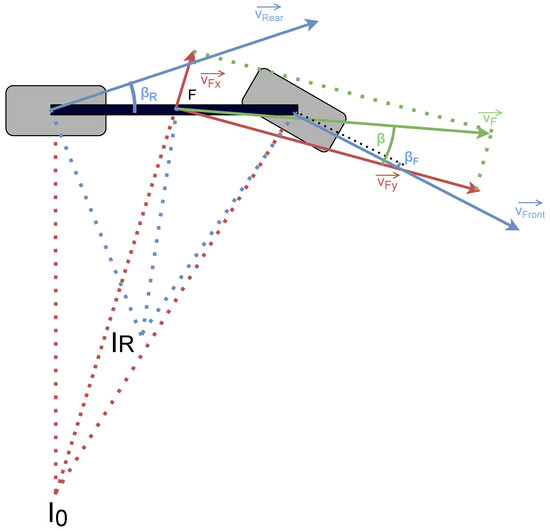
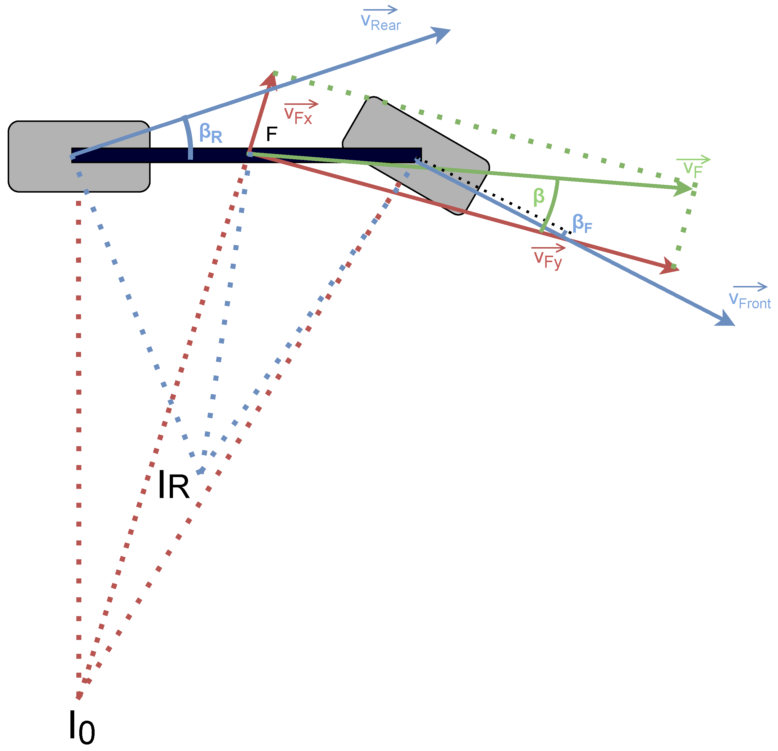
where is the longitudinal speed and is the lateral speed of the vehicle. The definition of the sideslip angle is illustrated in Figure 1. is the ideal instantaneous centre of rotation, is the ideal longitudinal speed vector and is the lateral speed component at the reference point (F). The vector describes the real longitudinal speed vector, and the corresponding sideslip angle is the angle between the ideal and real longitudinal speed vectors. When we draw the Ackermann steering geometry diagram, we can clearly observe that the real instantaneous centre of rotation has shifted, resulting in the respective sideslip angles and .
Figure 1.
Sideslip angle illustration (own illustration, based on [2]).
However, sensors that can directly measure the sideslip angle are expensive and not suitable for everyday driving conditions. Consequently, various estimation techniques have been developed for this purpose [3]. These methods can be divided into three main categories [1]:
- Kinematics-based methods (suitable for high velocities);
- Dynamics-based methods (suitable for low velocities, linear region);
- Neural network-based methods (perform well for all manoeuvres if dataset properly selected).
Neural network-based methods are a promising way of estimating sideslip angle, especially because of their universality. Various studies have been conducted for four-wheel vehicles [1], such as [4,5,6,7,8]. The majority of these studies use feedforward neural networks, but time-delay [7], recurrent-type (GRU—gated recurrent unit) [8], and NARX-NN [1] solutions have also been proposed.
The estimation of the sideslip angle in the case of powered two-wheelers (PTWs) is a much less discussed topic [3]. Several observer-based methods have been presented, such as those in references [9,10]. The work in [11] is also worth mentioning. This work presents an alternative, model-free method for estimating the sideslip angle of PTWs using a combination of inertial measurement unit (IMU) and monocular camera data. However, only one piece of work has been found by the author of this paper so far in the area of black-box/neural network-based approaches.
Ref. [3] presents a black-box, neural network-based estimation of the sideslip angle for PTWs. This study introduces three neural networks with different inputs: the ‘baseline’ network has an input vector, defined as [, , , , , , , ], where is the acceleration vectors in the respective axes, is the angular rotations around the respective axes, is the rear wheel velocity, and is the motorcycle’s velocity.
Furthermore, network has an input vector [, ], where is the roll angle; and network has an input vector [, ], where is the steering angle. The network achieved the lowest root mean square error (RMSE). The study also included a sensitivity analysis, which showed that performance varied most when the neural network input tensor did not include the and data.
All of the above work on vehicle sideslip estimators using neural network-based observers lacks a rigorous approach to computational and hardware resource utilisation and only states the sampling frequency of the acquired signal (without further explanation). The study in [6] proposes the use of the principal component analysis (PCA) technique for dimensionality reduction, and the study in [3] presents a sensitivity analysis of the model used. However, overall, the optimisation of signal selection, sampling, and embedding has not been rigorously studied in this particular area, as far as the author is aware.
However, this is a key factor in the adoption of neural network-based observers, since they are usually more computationally demanding than other regression methods. According to a comparative study [1], neural network-based estimators unfortunately remain far from being widely applicable to ECUs due to their computational requirements.
The aim of this work is to present a methodology for designing the optimal NARX-NN model, utilising an information theory and dynamic system reconstruction approach to optimise the selection and utilisation of hardware and computational power.
The purpose of this work is not to design a critical-response solution, given that motorcycle cornering ABS (anti-lock brake system) must respond much more quickly, at a frequency of around 100 Hz [12]. Instead, the goal is to design a ‘baseline provider’ system that can provide a high-accuracy, low-frequency state estimate in order to correct a high-frequency/lower-precision solution, which is only effective during brief and critical moments. A similar ‘two-stage’ solution for estimating motorcycle lean angle is presented in [13], for example.
2. Materials and Methods
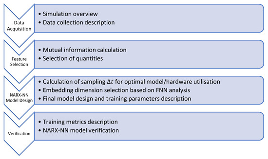
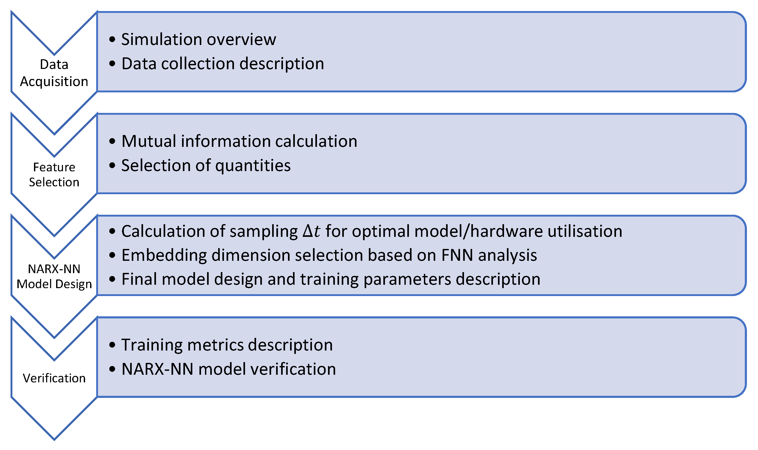
The methodology section is divided into four main parts, as illustrated in Figure 2:
Figure 2.
Overview of the used methodology.
- Data acquisition;
- Feature selection;
- NARX-NN model design;
- Verification.
The first part presents the use of high-fidelity simulation software for training and test dataset acquisition. Other important details regarding the simulation scenario, test track, manoeuvre description, and data acquisition process are provided.
The second part describes a feature selection process, where the main metric for feature selection is the mutual information between the observed quantity and the candidate input quantities. The final quantities are then selected based on the simplicity of the measurement (i.e., installed on-board sensors).
The third part presents an optimal embedding dimension for ensuring dynamics reconstruction, based on the Takens’ embedding theorem. Furthermore, the optimal sampling frequency is determined by calculating the mutual information/time-delay ratio.
The final section presents an evaluation of the trained model. The trained model is assessed using a validation dataset and is compared to an alternative observer solution, while the control metrics root mean squared error (RMSE), mean squared error (MSE), and mean absolute error (MAE) are calculated.
2.1. Data Acquisition
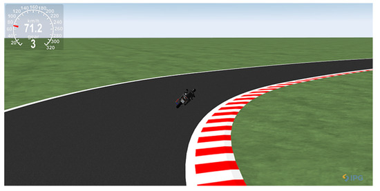
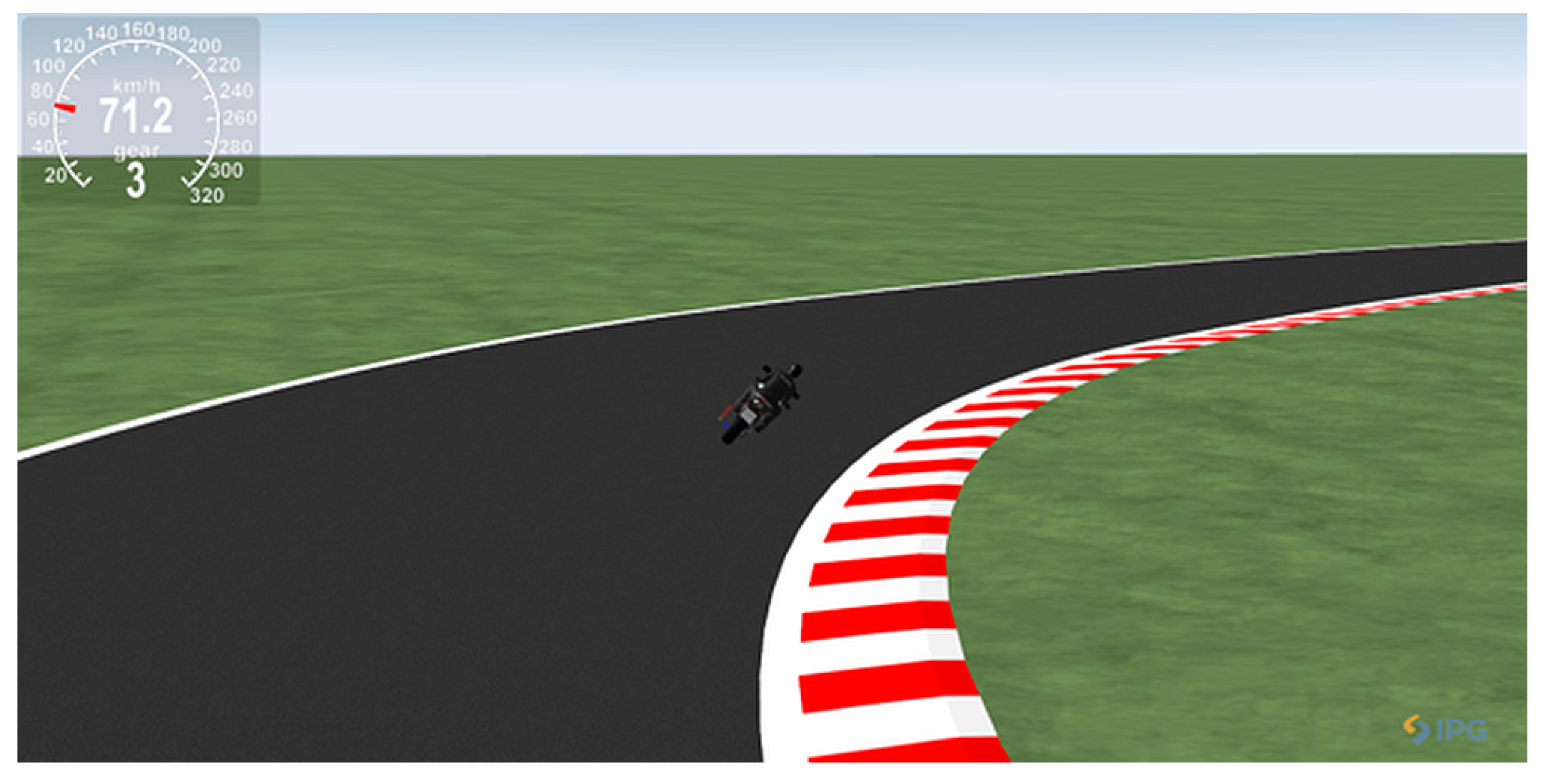
A high-fidelity motorcycle simulator (IPG MotorcycleMaker, Karlsruhe, Germany, version 14.0.1) was used for data acquisition [14]. This simulation software is an industrial-standard solution for modelling and simulating two-wheelers, and has been used in a variety of studies, including those related to stability issues [15]. An example of the graphical output from this simulation software is shown in the Figure 3.
Figure 3.
Virtual simulation scene in IPG MotorcycleMaker.
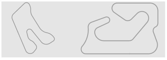
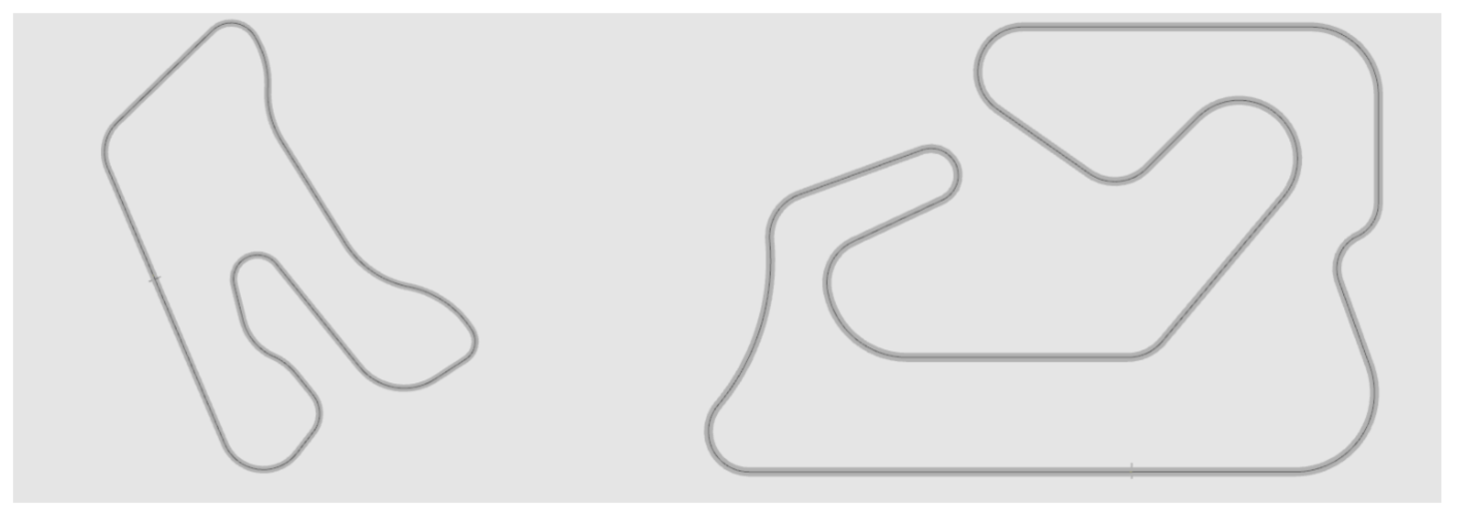
Two generic scenarios were used for the study. A ‘Hockenheim’scenario was used to acquire the training dataset. The testing dataset was obtained using the ‘Albacete’ scenario. Circuits used to create the training and test datasets are shown in the Figure 4.
Figure 4.
Hockenheim (left) and Albacete (right) circuit scenarios.
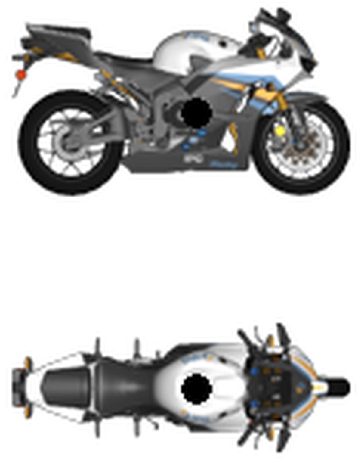
For both experiments, the same generic motorcycle model ‘DemoMC_Honda’ was used during the study. This model uses typical but unvalidated values for a generic sports motorcycle, serving as a good generic baseline multibody model for data analysis. The reference point F is presented in Figure 5.
Figure 5.
Motorcycle and reference point of the measurement.
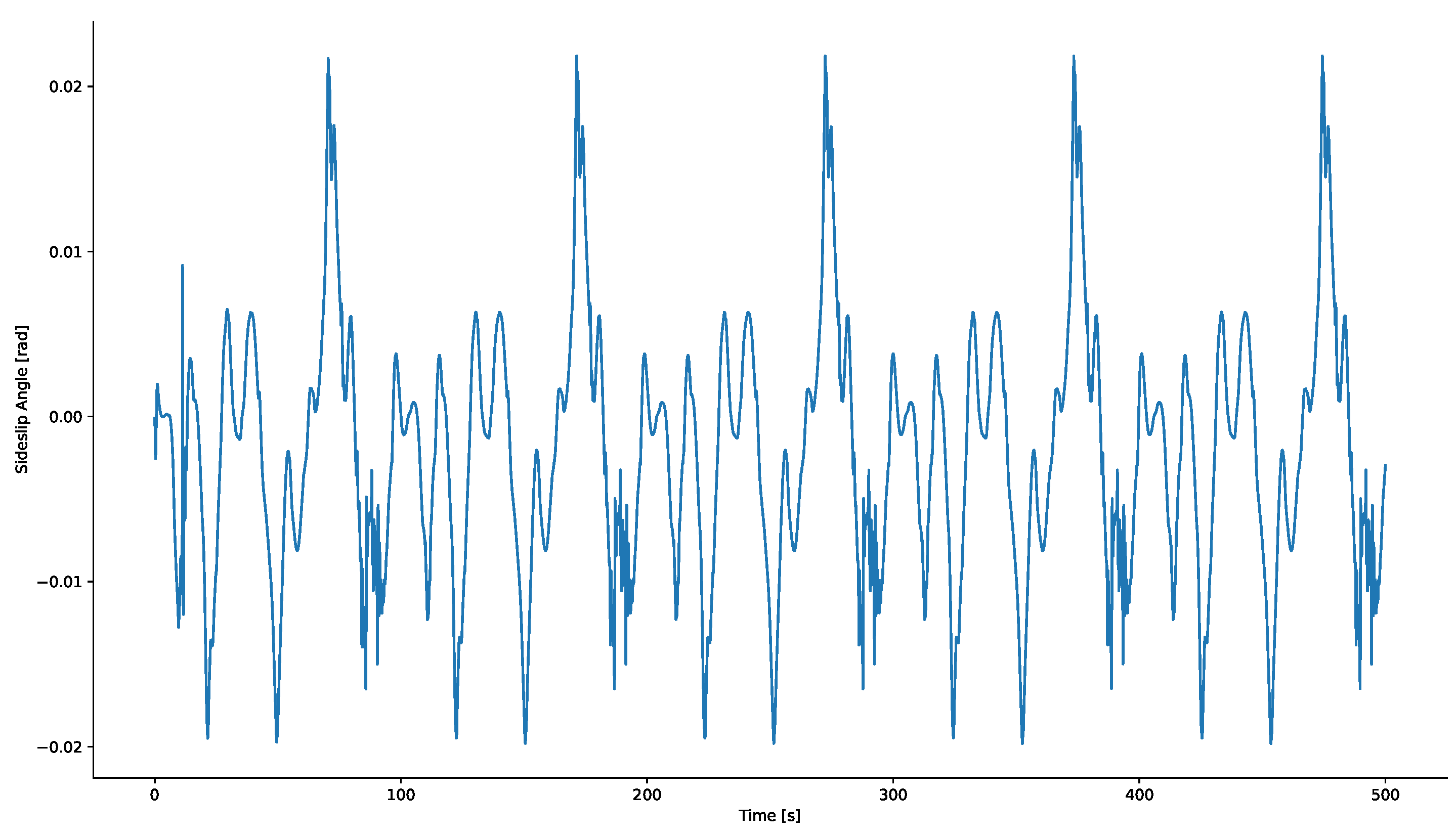
All available simulation data were collected with a sampling frequency of 100 Hz (sampling period: 0.01 s). Output values for the sideslip angle in the Hockenheim scenario (training dataset) are presented in Figure 6.
Figure 6.
Sideslip values for Hockenheim scenario.
The basic data for the training dataset (with respect to the quantities discussed in the next section) are listed in Table 1.
Table 1.
Key characteristics of the training dataset.
2.2. Calculation of Mutual Information Between Time-Series Data
Mutual information (MI) is a metric used in nonlinear system identification. It is crucial in determining whether the measured variable has contributed to the value estimated by the virtual sensor (i.e., the observer). In other words, it shows how much information about the target variable can be obtained from the observed variable [16].
The mutual information between two variables, X and Y, can be described as follows [16]:
for marginal distributions of and .
The mutual information between two Gaussian distributions can be demonstrated by the following equation, which describes the relationship between mutual information and Pearson’s product-moment correlation [17,18]:
where is the mutual information in nats for the given Gaussian distributions, and r is the Pearson product-moment correlation coefficient for the sample. However, this equation only works for time series with a Gaussian distribution and linear correlation [18,19]. Therefore, the equation only provides a virtual representation of the correlation that would be observed if the time series had the aforementioned characteristics. To calculate the mutual information between two general time series, we need to use Equation (2). From Equation (3), we can derive the equivalent of Pearson’s product-moment correlation as follows:
In this paper, mutual information estimation was performed using the scikit-learn library and the ‘mutual_info_regression’ function [20], based on [17]. This paper presents an alternative, more robust approach to estimating mutual information based on k-nearest neighbour distances for entropy estimation. Details of the implementation can be found in the paper. The calculated mutual information between the sideslip angle and all the measured quantities (in nats) is provided in the Supplementary Materials.
2.3. Selection of Model Input Quantities
The suitable input quantities were selected based on the calculated mutual information using the predicted sideslip angle mentioned above. Since it is impossible to calculate the joint mutual information (JMI) for all sensor combinations due to the curse of dimensionality, it was necessary to reduce both the number of input variables and the size of the sensor set. This was achieved using the following procedure:
- Selection of the top 100 variables based on mutual information (excluding self-mutual information);
- Removing duplicate signals;
- Removing signals that are not scenario-agnostic (such as the motorcycle’s position within the simulation, or wind direction);
- The final sensor set is selected using qualitative assessment.
The output of step 3 consists of the candidate variables shown in Table 2.
Table 2.
Overview of candidate quantities.
Based on this table, the most sensible option is to use the built-in IMU installed for cornering ABS, which is becoming increasingly popular in the motorcycle industry due to its safety benefits [24].
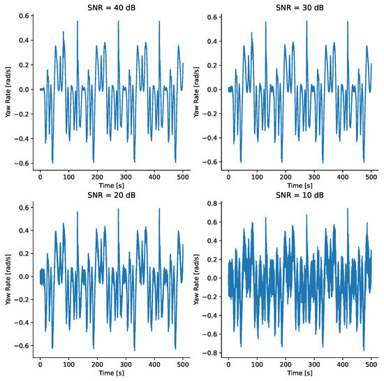
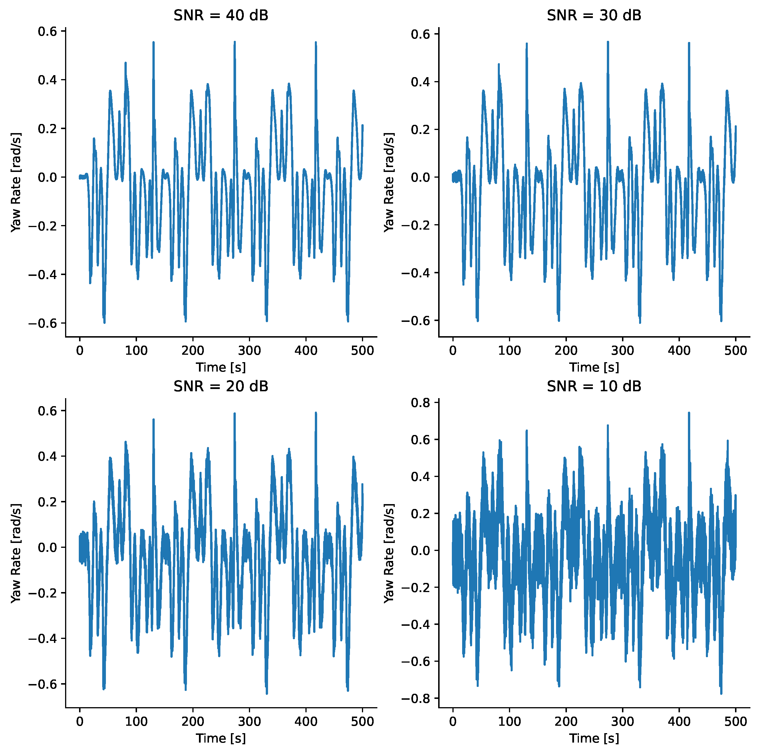
Conducting a full verification solely of ‘clean simulator data’ was inconclusive. To this end, the data from various tests was corrupted with different signal-to-noise ratios (SNRs). Figure 7 shows an example of the variable with different levels of noise.
Figure 7.
Signal with varying levels of noise.
As part of the experiment, the joint mutual information was calculated for clean data from the simulator and for data with noise at SNRs of 40 and 10 dB. The results are summarised in Table 3.
Table 3.
JMI for various combinations of candidate quantities.
Based on this finding, it is clear that merging the IMU measurements does not provide any additional information, even for highly noisy data. Since including more inputs would increase the number of parameters in the resulting NARX-NN model, only one variable was selected. Although centripetal acceleration provides slightly more information, yaw rate was chosen for the experiment because it is a directly measured quantity, so there is no cumulative error caused by an additional observer. This finding also correlates with the results of the study in [3], which considers roll rate and yaw rate to be the quantities that contribute most to the proposed estimator, based on a sensitivity analysis.
2.4. Identification of Optimal Sampling Frequency
The simulation data in the dataset were sampled at a frequency of 100 Hz, meaning the time interval between measured values is 0.01 s. Since neural network-based models are computationally demanding, running them at this frequency can be challenging for low-power ECUs. The aim is to find the optimal delayed mutual information in order to correctly reconstruct the dynamics of the system by estimating the time delay between state estimations. In practice, the most commonly used method is to find the first minimum of the so-called delayed mutual information [25].
The NoLiTSA (Non-Linear Time Series Analysis) library [26] was used for the delayed mutual information. The local minimum was then found in the smoothed delayed mutual information graph, which was filtered using a Savitzky–Golay filter [27] with a window length of 10 and a polyorder of 2.
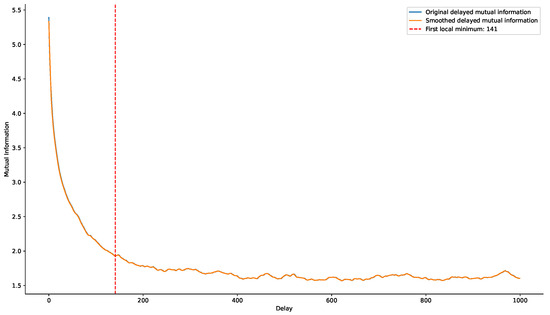
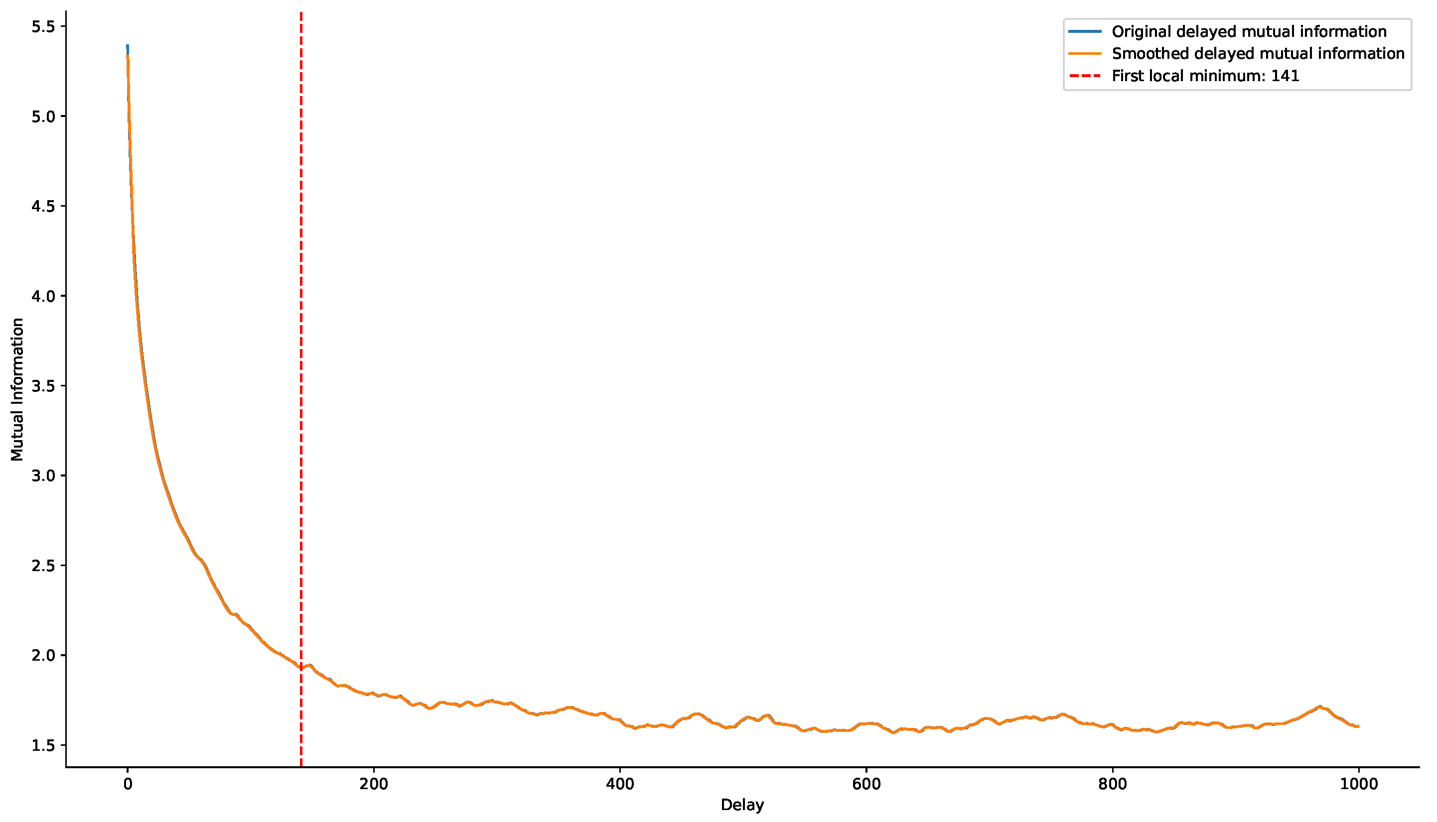
As shown in Figure 8, the original output of the simulation is greatly oversampled. The first local minimum for the smoothed, delayed mutual information lies at 141, which is much higher than the recommended value. According to [28], good control system performance is achieved by sampling at a rate between 10 and 30 times the sampled system’s bandwidth.
Figure 8.
First local minima for /MI dependence.
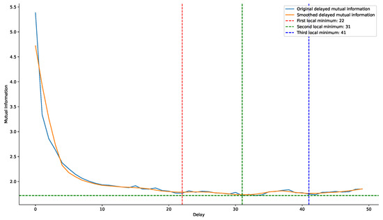
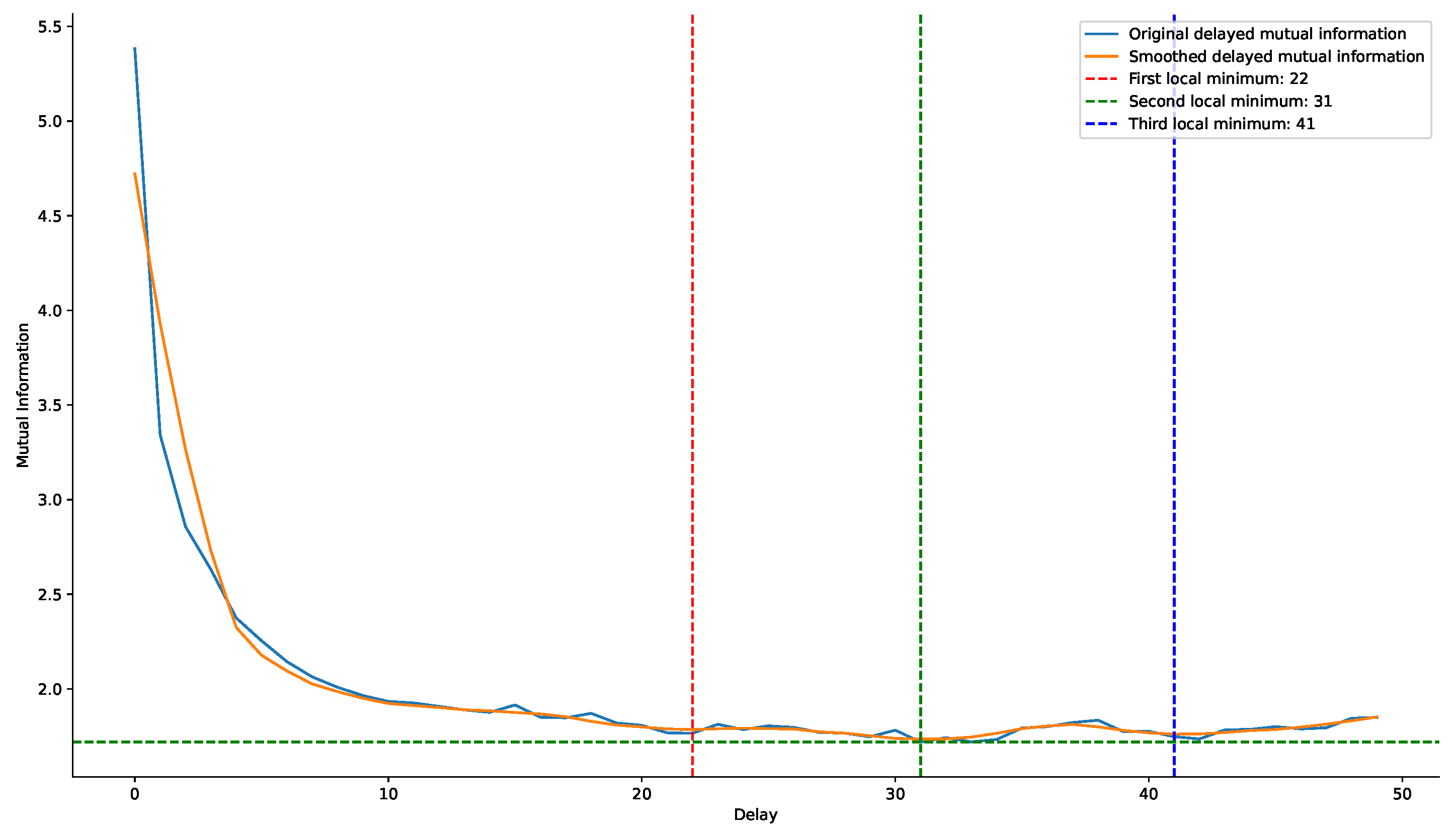
As can be seen in Figure 9, when we down-sample 20 times at a sampling frequency of 5 Hz ( = 0.2 s), we find the first local minimum in the filtered signal at = 22, and the global minimum on the interval [] lies at a delay of 31. As these values are close to the optimal interval, the sampling frequency is set to 5 Hz.
Figure 9.
dependence for down-sampled signal.
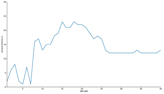
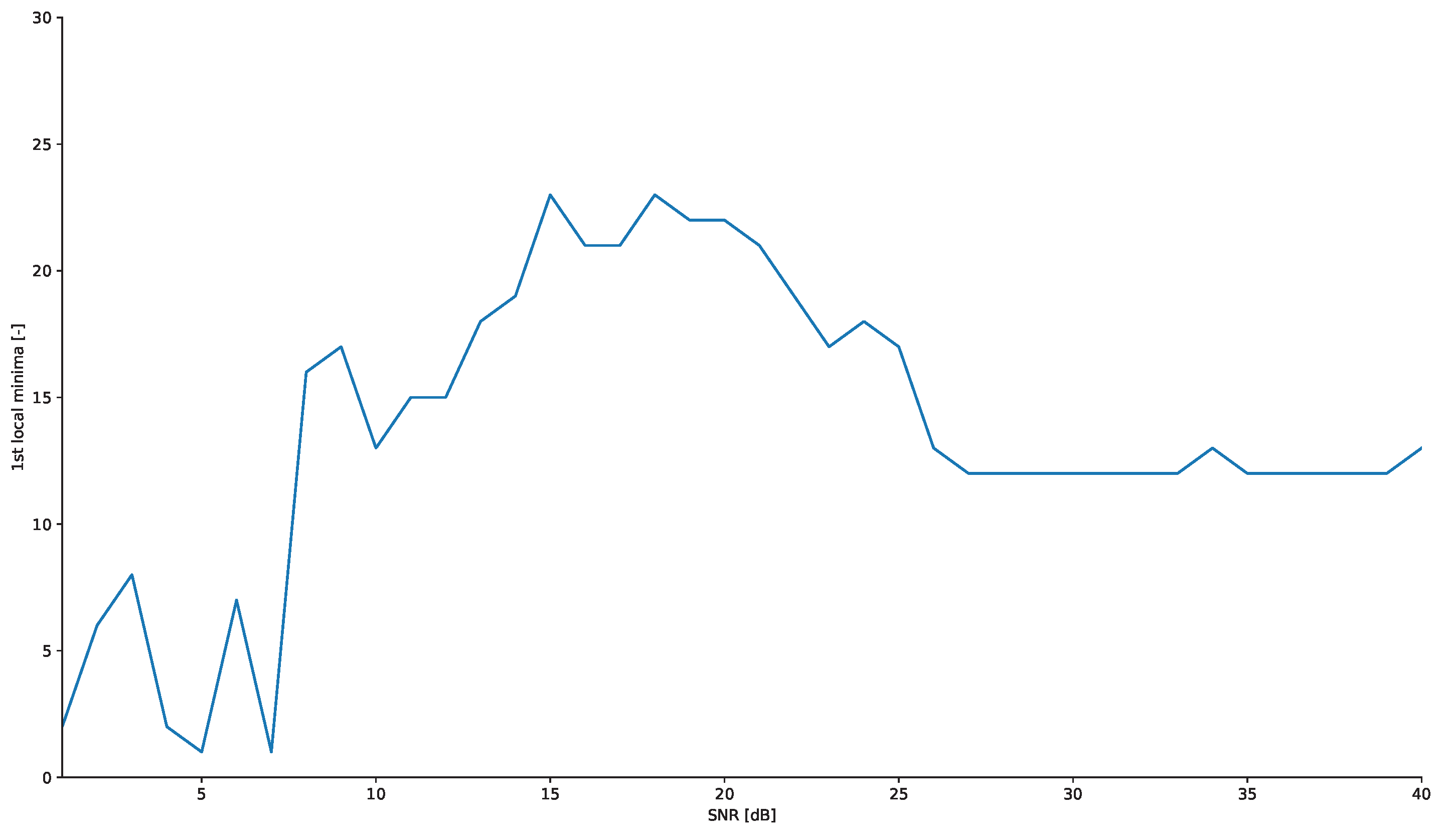
The location of the first local minimum was calculated for a signal with varying noise levels, ranging from pure noise (SNR = 0 dB) to an SNR of 40 dB. The location of the first local minimum of the delayed mutual information for various noise levels is shown in Figure 10.
Figure 10.
Location of the first minimum of MI based on the signal-to-noise ratio.
2.5. Calculation of Embedding Dimension
Let us assume that the motorcycle dynamics system under study has the Markov property, meaning that the system is memoryless. Based on this assumption, the system’s next state depends solely on its current state and the current external input [29,30]. We can describe the Markov property as follows:
The Markovian property is crucial for approximating dynamics using feedforward neural networks. However, determining the full system state using only sensors can lead to redundancy and be affected by noise, for example. An alternative way to determine the system state is to use a model with memory. The above-mentioned literature discusses three possible approaches for determining the sideslip angle (but these are not an exhaustive list of possibilities):
- Recurrent neural networks with hidden states (in this case GRU, but can also be LSTM or simple RNN) [8];
- Time-delay neural networks [7];
- NARX-NN models [1].
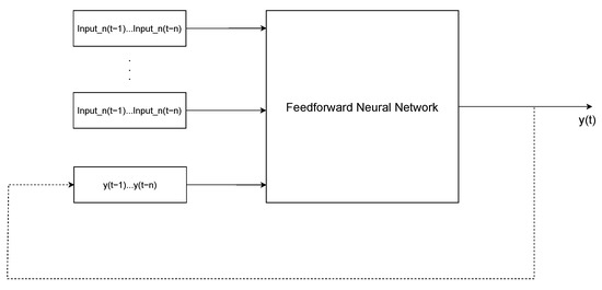
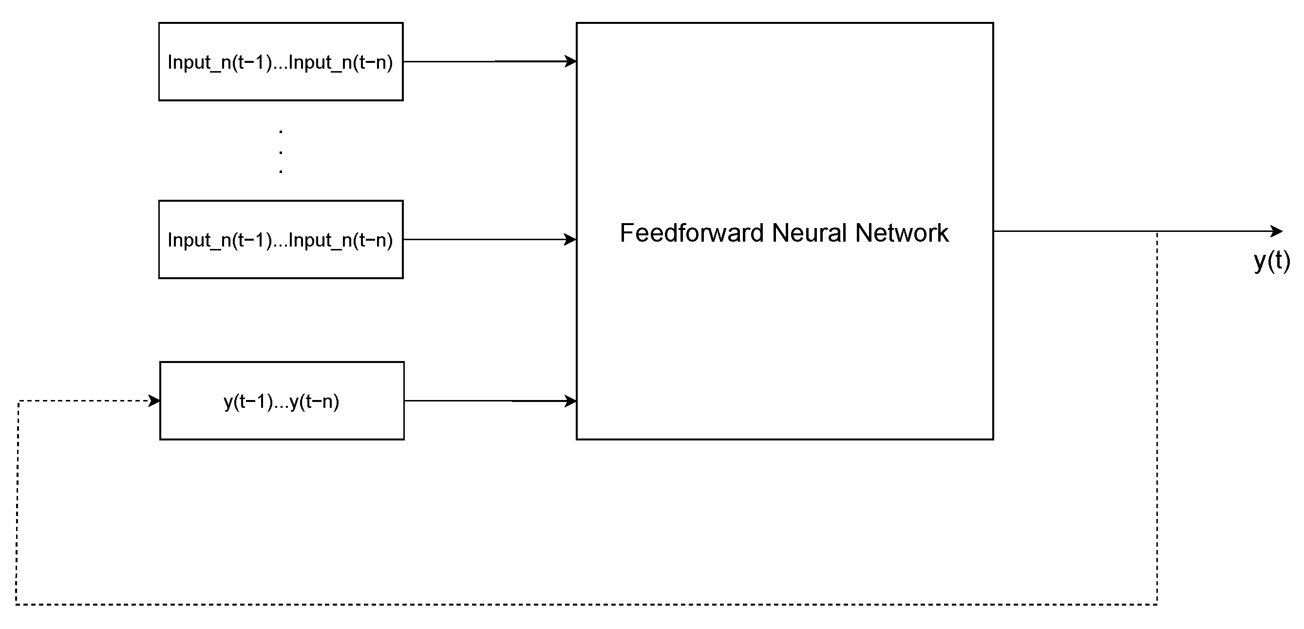
This work uses a NARX-NN model. The advantage of using a feedforward neural network instead of a recurrent network with hidden states is that it generally has lower computational demands, making it suitable for low-power ECUs. This topic is discussed in more detail in Appendix A. However, since it does not have an internal hidden state (‘memory’), it is necessary to provide information about previous states and inputs in order to reconstruct the underlying dynamics of the modelled system. The general architecture of the NARX-NN model is presented in Figure 11.
Figure 11.
General NARX-NN architecture.
To optimally reconstruct the dynamics of a partially observable system, it is necessary to determine the optimal embedding dimension n, which indicates the number of steps backwards (also known as ‘look-ahead’ or ‘embedding’) required to obtain sufficient information for state-space reconstruction. According to Takens’ theorem, the embedding dimension n is defined as follows [31]:
where m is the system’s attractor phase-space dimension (embedding dimension) [32]. One of the most commonly used methods for determining the dimension m is the so-called ‘false nearest neighbour’ (FNN) method. We assume that, in lower dimensions, two points in embedding dimension m appear closer together. If the distance between these points does not change as the dimension increases, they are not false nearest neighbours [25].
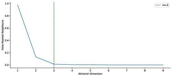
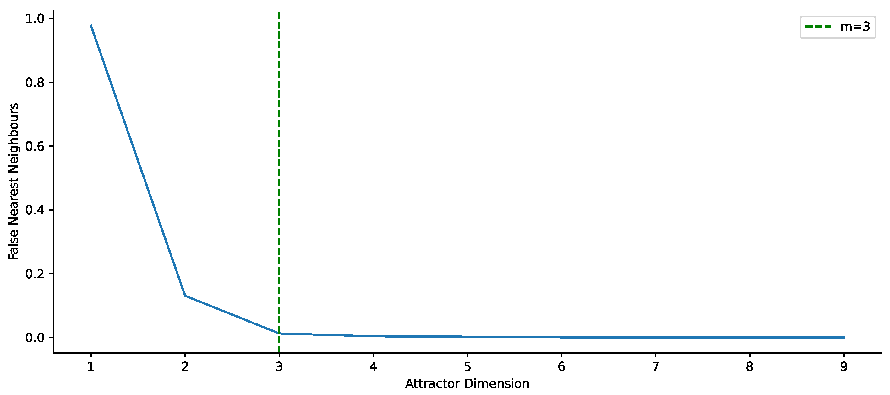
The false nearest neighbours were calculated using the NoLiTSA library [26], which utilises Kennel’s algorithm [33]. Our general aim is to achieve a false nearest neighbour percentage of zero; however, for noisy data, our aim is to reach the dimension at which the rapid decrease stops (where the knee-point appears) [25]. Figure 12 shows how the number of false nearest neighbours drops significantly at the knee-point at and then stops. Based on this graph, we determined the embedding dimension to be .
Figure 12.
Number of false nearest neighbours based on dimension m (the green line represents the optimal attractor dimension for embedding).
2.6. Final Design of NARX-NN Observer
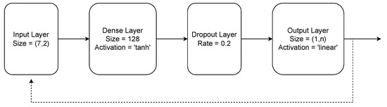
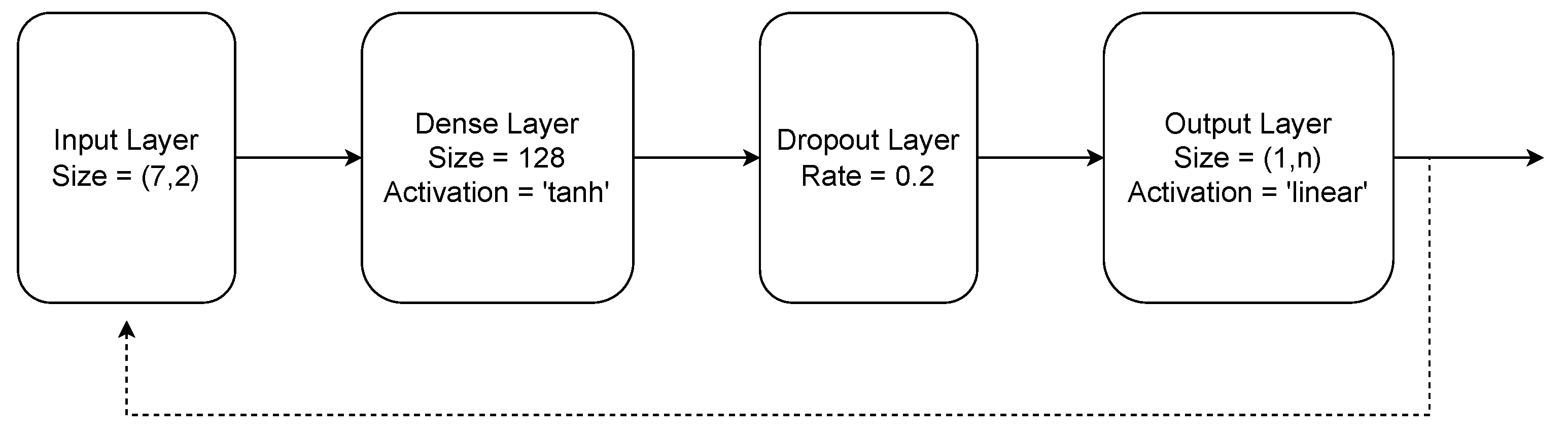
The NARX-NN observer was derived based on the above-mentioned experiments. The observer was created using the Keras library [34] with the Sequential API (application programming interface). The general architecture of the observer is presented in Figure 13. The dimension n in the last layer represents the number of forward passes (horizon). In this experiment, was chosen to increase the stability of model training on noisy data.
Figure 13.
Proposed NARX-NN model architecture.
The testing model was trained in so-called ‘series–parallel’ mode. This means that the neural network was trained solely on measured data, and the loss function calculated does not assess performance using its own feedback loop. Although ‘parallel training’, where the feedback loop is used during training, can provide better results in some circumstances (e.g., noisy environments), the series–parallel approach is currently still considered the best practice in the field due to its simplicity, higher degree of parallelisation, and reduced risk of becoming stuck in a non-optimal local solution [35]. The training parameters are presented in Table 4.
Table 4.
Training options of the observer.
2.7. Disclaimer on GenAI Use
During the preparation of this study, the author used Google Gemini (3, 3.1 Pro, 3.1 Flash-Lite and 3.5 Flash) for the purposes of assistance with coding tasks. After using this tool, the author thoroughly reviewed, executed, and validated all generated code to ensure its accuracy. The author has reviewed the output and takes full responsibility for its validity.
3. Results
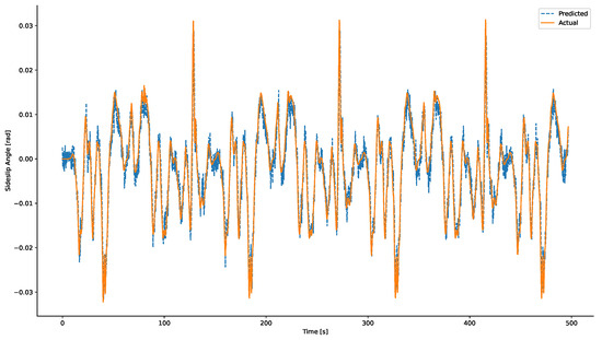
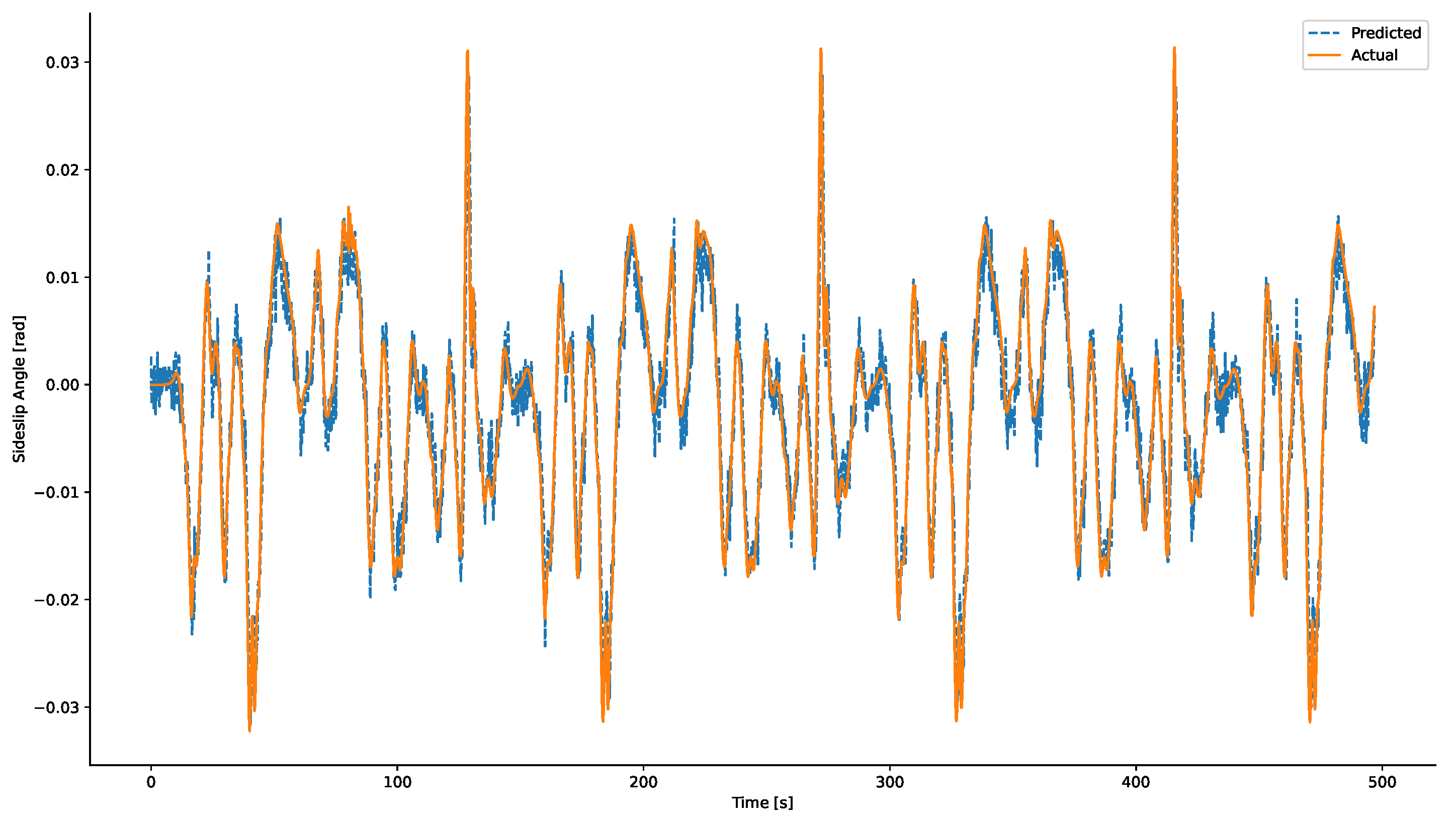
The observer was tested on the evaluation dataset (Albacete) with the same sampling. In this case the observer was run in parallel mode (with feedback). However, testing of the virtual sensor on noise-free data from a simulator did not provide sufficiently convincing evidence of performance under real-world operating conditions. The proposed virtual sensor was therefore tested on a noisy signal with an SNR of 10 dB. The results are shown in Figure 14.
Figure 14.
A comparison of the prediction of the NARX-NN model with the actual data.
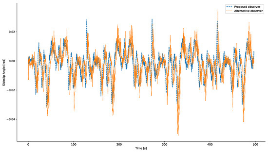
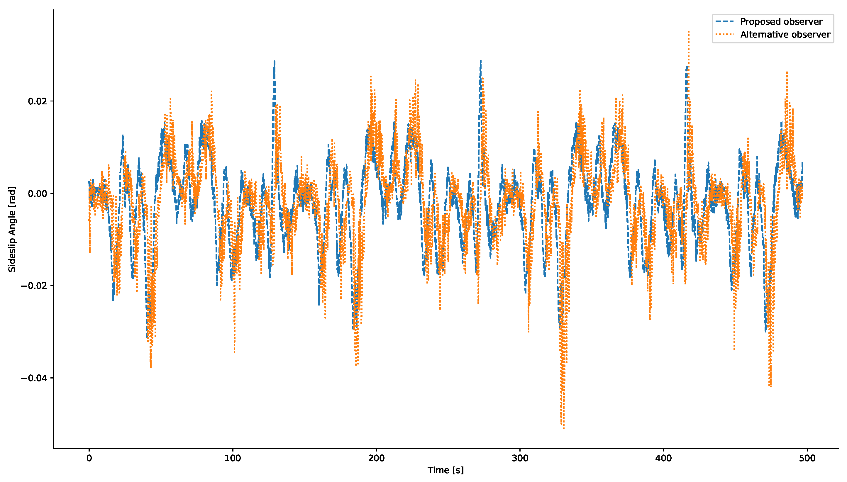
The model was also compared on the same test dataset with SNR = 10 dB against an observer published in [10]. Figure 15 shows a comparison of the sideslip angle estimates for the proposed model and the alternative observer with the same SNR of input signals.
Figure 15.
A comparison of the prediction of the NARX-NN model with an alternative observer.
The difference between reality and the prediction was tested using the MSE [36], RMSE [37], and MAE [38] metrics. The results are presented in Table 5.
Table 5.
Validation metrics for simulation data.
4. Discussion
The use of information theory in the synthesis of a virtual sensor for sideslip angle reconstruction has demonstrated its ability to reduce the computational burden on ECUs in neural network-based observer applications. Based on time-delayed mutual information, the sampling frequency can be reduced by up to 20 times while still providing a sufficient prediction approximation for non-critical tasks. Mutual information between the target quantity and the candidate input quantities was utilised to easily select an input channel with the most non-redundant information.
An interesting finding of this study is that, even though the sideslip angle depends directly on the longitudinal and lateral speed, and longitudinal speed is used as the input quantity in the majority (if not all) of estimation models, the model can still work robustly without direct information about the PTW speed. This can be explained by the following assumption: centripetal force is defined as [3]
where M is mass, is the longitudinal speed, and R is the turning radius. An alternative formula for calculating the centripetal force with the yaw rate is given in [39]:
where M is mass, R is the turning radius, and is the yaw rate. Therefore, we can write
and
Therefore, the yaw rate carries more information than just the longitudinal speed itself for estimating motorcycle sideslip. Of course, we must take into account that the motorcycle is leaning into curves, so the yaw rate changes during manoeuvres. The roll angle of the centre of mass of the motorcycle–rider system (if bike’s roll angle ≅ rider’s roll angle) is defined as follows [40]:
This shows that the roll angle carries information that differs only slightly from the yaw rate information that is already known. When provided with a reference to its previous state (using embedding), a neural network can use this latent information to reconstruct the dynamics of a known motorcycle.
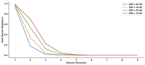
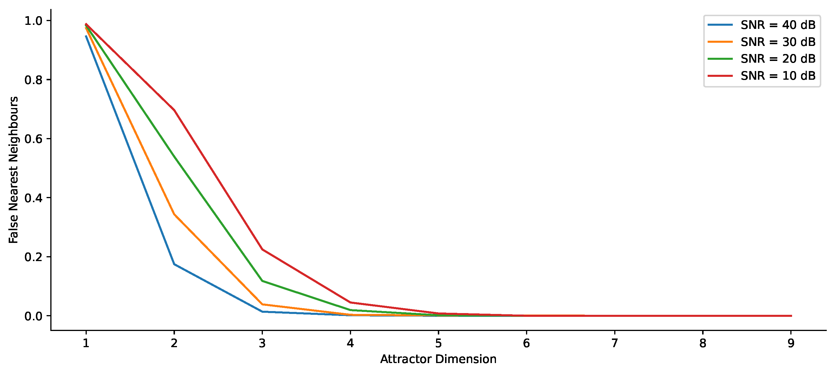
It is important to note that although the embedding chosen in the presented architecture has been validated using FNN analysis, other potential factors must also be taken into account. The first of these is the effect of noise, which can influence the required length of the embedding window. An analysis of the effect of noise on the autoregressive component is presented in Figure 16.
Figure 16.
FNN analysis based on various noise levels.
Although the increased noise level in this component may require a longer embedding, analysis of the autoregressive component shows an SNR of 20.7 dB, even for a heavily noisy signal from the IMU with an SNR of 10 dB. This is due to the fact that the NARX-NN model behaves as a nonlinear filter (it depends on the values in the previous n steps), so even for a significantly noisy input signal from the sensor, its output (and consequently the model’s autoregressive component) will exhibit lower noise [41]. Even with such a noisy signal, the model achieves very good results with the selected seven-step tapped delay window. For practical use with most modern sensors, this embedding should be sufficient.
Another limitation is that this is a black-box model that has been tested on only one test dataset. However, the original assumption (that the system is Markovian), combined with the FNN and DMI analyses performed (to determine the required sampling frequency and embedding), may not be universally valid. In certain cases, unobserved dynamic dependencies (which were not included in the training dataset) could lead to the need for a longer embedding window to fully reconstruct the motorcycle’s dynamics.
5. Conclusions
This paper proposes an alternative approach to synthesising a NARX-NN-based virtual sensor for estimating sideslip angles in PTW applications. This approach is based on information theory and aims to utilise the ECU’s computational resources optimally while providing the virtual sensor with enough information to robustly reconstruct motorcycle dynamics. Predictions on the test dataset demonstrate robust performance, with , , and for data with = 10 dB. The proposed approach also has economic potential, since it enables the installation of a less powerful (and usually cheaper) ECU to obtain the same results.
The limitations of the study lie in the absence of real-world measurements and the fact that it relies solely on a simulation study. However, a high-fidelity, industrial-grade simulator with added noise was used. Future work will focus on testing the NARX-NN model using highly noisy or sparse/incomplete datasets. Future work will also focus on validating the hypothesis regarding the embedding window length across a wide range of driving scenarios and situations, in order to confirm the practical applicability of the embedding window presented in this paper.
Supplementary Materials
The following supporting information can be downloaded at: https://www.mdpi.com/article/10.3390/vehicles8070161/s1.
Funding
This contribution is supported by the internal project SGS-2025-003—Advanced Construction Methods using Numerical Simulations and Alternative Materials.
Data Availability Statement
Supplementary data are available in the Figshare repository, which is accessible via the following DOI link: https://doi.org/10.6084/m9.figshare.32012433.
Acknowledgments
The author would like to thank IPG Automotive for providing him with a non-commercial license for IPG MotorcycleMaker to conduct this work. During the preparation of this study, the author used Google Gemini (3, 3.1 Pro, 3.1 Flash-Lite and 3.5 Flash) for the purposes of assistance with coding tasks and to improve the readability and language of the manuscript. Also, DeepL and DeepL Write were used to improve the readability and the language of the manuscript. The author has reviewed and edited the output and takes full responsibility for the content of this publication.
Conflicts of Interest
The author declares no conflicts of interest.
Abbreviations
The following abbreviations are used in this manuscript:
| ABS | Anti-lock Braking System |
| ADAM | Adaptive Moment Estimation |
| ADAS | Advanced Driver-Assistance System |
| API | Application Programming Interface |
| ARAS | Advanced Rider-Assistance System |
| ECU | Electronic Control Unit |
| FLOP | Floating Point Operation |
| FNN | False Nearest Neighbour |
| GRU | Gated Recurrent Unit |
| IMU | Inertial Measurement Unit |
| JMI | Joint Mutual Information |
| LSTM | Long Short-Term Memory |
| MAC | Multiply-Accumulate |
| MAE | Mean Absolute Error |
| MATLAB | Matrix Laboratory |
| MI | Mutual Information |
| MLP | Multilayer Perceptron |
| MSE | Mean Square Error |
| NARX | Nonlinear Autoregressive Model with Exogenous Inputs |
| NARX-NN | Nonlinear Autoregressive Neural Network with Exogenous Inputs |
| NoLiTSA | Nonlinear Time Series Analysis |
| PCA | Principal Component Analysis |
| PTW | Powered Two-Wheeler |
| RMSE | Root Mean Square Error |
| RNN | Recurrent Neural Network |
Appendix A. Discussion on Computation Efficiency
The purpose of this appendix is to compare the proposed feedforward neural network with recurrent alternatives (in this case, “vanilla” RNNs, GRUs, and LSTMs). This discussion is crucial for identifying the optimal variant in terms of hardware resource utilisation.
From the perspective of computational complexity, the fundamental arithmetic operation in the field of neural networks is the multiply–accumulate (MAC) operation. It is defined as adding the dot product of b and c to the base variable (a). This operation can be written as follows [42]:
An alternative method is to use floating-point operations (FLOPs), where . To calculate the number of MAC operations required for a given layer of a neural network, one can refer to [43]. The computational complexity for each layer is summarised in Table A1, where
- is the number of neurons;
- is the number of features in the input vector;
- is the input sequence size;
- is the number of hidden units.
Table A1.
MAC calculation for given layers [43].
For the overall calculation, it is therefore necessary to consider not only the neurons in the hidden layer, but also the neurons in the output layer. The NARX-NN model has (as mentioned earlier) seven output neurons, while recurrent models always have only one neuron in the output layer. At the same time, the MLP model has fourteen inputs (seven exogenous and seven autoregressive), while the recurrent models have only seven inputs.
For the purposes of this study, we compared how large individual recurrent models could be in order to be computationally comparable to the proposed NARX-NN model. The respective model specifications are shown in Table A2.
Table A2.
Specifications of compared networks.
A comparison of the number of MACs for each of the networks under comparison is shown in Table A3. This is a partially simplified calculation—this simplified analysis does not take into account the computational overhead of activation function calculation. These calculations vary depending on whether the functions are linear or nonlinear (e.g., tanh) and vary significantly based on the target hardware and final implementation.
Table A3.
MAC count for compared networks.
The number of parameters was also calculated for these networks. The formulas for calculating the number of parameters for each layer are shown in Table A4. The equation for calculating the MLP was taken from [44], and the equation for recurrent architectures from [45].
Table A4.
Parameter calculation for given layers [44,45].
The total number of parameters for each type of network is listed in Table A5.
Table A5.
Parameter count for compared networks.
Given the number of parameters and the number of FLOPs/MACs, it is possible to calculate the arithmetic intensity of the network. This is defined by the formula [46]
Since recurrent networks process data sequentially, the sum of the number of parameters for these networks must be multiplied not only by the number of bytes per parameter, but also by the length of the sequence to obtain the denominator. The results for each type of network (considering 4 bytes per parameter) are shown in Table A6.
Table A6.
Arithmetic intensity of compared networks.
The data in Table A6 show that the proposed NARX-NN multilayer perceptron model offers higher arithmetic intensity than comparable networks (from a MACs/FLOPs point of view) based on recurrent architectures.
References
- Liu, J.; Wang, Z.; Zhang, L.; Walker, P. Sideslip Angle Estimation of Ground Vehicles: A Comparative Study. IET Control Theory Appl. 2020, 14, 3490–3505. [Google Scholar] [CrossRef] [Scilit]
- Pneumatici, Motorcycle, Tires, Tyres. Available online: https://www.dynamotion.it/dinamoto/8_on-line_papers/Pneumatici/Pneumatii_eng.htm (accessed on 9 June 2026).
- Busnelli, F.; Panzani, G.; Corno, M.; Savaresi, S.M. Two-Wheeled Vehicles Black-Box Sideslip Angle Estimation. In 2017 IEEE 56th Annual Conference on Decision and Control (CDC); IEEE: New York, NY, USA, 2017; pp. 351–356. [Google Scholar] [CrossRef] [Scilit]
- Du, X.; Sun, H.; Qian, K.; Li, Y.; Lu, L. A Prediction Model for Vehicle Sideslip Angle Based on Neural Network. In 2010 2nd IEEE International Conference on Information and Financial Engineering; IEEE: New York, NY, USA, 2010; pp. 451–455. [Google Scholar] [CrossRef] [Scilit]
- Chindamo, D.; Gadola, M. Estimation of Vehicle Side-Slip Angle Using an Artificial Neural Network. MATEC Web Conf. 2018, 166, 02001. [Google Scholar] [CrossRef] [Scilit]
- De Martino, M.; Farroni, F.; Pasquino, N.; Sakhnevych, A.; Timpone, F. Real-Time Estimation of the Vehicle Sideslip Angle through Regression Based on Principal Component Analysis and Neural Networks. In 2017 IEEE International Systems Engineering Symposium (ISSE); IEEE: New York, NY, USA, 2017; pp. 1–6. [Google Scholar] [CrossRef] [Scilit]
- Liu, J.; Wang, Z.; Zhang, L. A Time-delay Neural Network of Sideslip Angle Estimation for In-wheel Motor Drive Electric Vehicles. In 2020 IEEE 91st Vehicular Technology Conference (VTC2020-Spring); IEEE: New York, NY, USA, 2020; pp. 1–5. [Google Scholar] [CrossRef] [Scilit]
- Gräber, T.; Lupberger, S.; Unterreiner, M.; Schramm, D. A Hybrid Approach to Side-Slip Angle Estimation with Recurrent Neural Networks and Kinematic Vehicle Models. IEEE Trans. Intell. Veh. 2019, 4, 39–47. [Google Scholar] [CrossRef] [Scilit]
- Dabladji, M.E.H.; Ichalal, D.; Arioui, H.; Mammar, S. Observer Based Controller for Single Track Vehicles. In 52nd IEEE Conference on Decision and Control; IEEE: New York, NY, USA, 2013; pp. 7420–7425. [Google Scholar] [CrossRef] [Scilit]
- Teerhuis, A.P.; Jansen, S.T. Motorcycle State Estimation for Lateral Dynamics. Veh. Syst. Dyn. 2012, 50, 1261–1276. [Google Scholar] [CrossRef] [Scilit]
- Alrazouk, O.; Chellali, A.; Nehaoua, L.; Arioui, H. Vision-Based Approach for Estimating Lateral Dynamics of Powered Two-Wheeled Vehicles. In 2023 American Control Conference (ACC); IEEE: New York, NY, USA, 2023; pp. 999–1005. [Google Scholar] [CrossRef] [Scilit]
- Motorcycle Stability Control (MSC). Available online: https://www.bosch-mobility.com/en/solutions/driving-safety/motorcycle-stability-control/ (accessed on 13 June 2026).
- Mimmo, N.; Zanzi, M. High-Performance Motorbike Lean Angle Estimation. IEEE Trans. Control Syst. Technol. 2025, 33, 1983–1994. [Google Scholar] [CrossRef] [Scilit]
- MotorcycleMaker | IPG Automotive. Available online: https://www.ipg-automotive.com/en/products-solutions/software/motorcyclemaker/ (accessed on 18 November 2025).
- More Stability with MotorcycleMaker. Available online: https://www.ipg-automotive.com/fileadmin/data/know-how/publications/case_studies/Success_Story_SI_MotorcycleMaker_EN.pdf (accessed on 4 March 2026).
- Learned-Miller, E.G. Entropy and Mutual Information. Department of Computer Science, University of Massachusetts, Amherst. Available online: https://people.cs.umass.edu/~elm/Teaching/370_F09/mutInf.pdf (accessed on 10 April 2026).
- Kraskov, A.; Stoegbauer, H.; Grassberger, P. Estimating Mutual Information. Phys. Rev. E 2004, 69, 066138. [Google Scholar] [CrossRef] [Scilit] [PubMed]
- Zeng, X.; Durrani, T.S. Estimation of Mutual Information Using Copula Density Function. Electron. Lett. 2011, 47, 493–494. [Google Scholar] [CrossRef] [Scilit]
- Pearson Product-Moment Correlation—When You Should Run This Test, the Range of Values the Coefficient Can Take and How to Measure Strength of Association. Available online: https://statistics.laerd.com/statistical-guides/pearson-correlation-coefficient-statistical-guide.php (accessed on 22 February 2026).
- Mutual_Info_Regression. Available online: https://scikit-learn/stable/modules/generated/sklearn.feature_selection.mutual_info_regression.html (accessed on 22 February 2026).
- Carputo, F.; D’Andrea, D.; Risitano, G.; Sakhnevych, A.; Santonocito, D.; Farroni, F. A Neural-Network-Based Methodology for the Evaluation of the Center of Gravity of a Motorcycle Rider. Vehicles 2021, 3, 377–389. [Google Scholar] [CrossRef] [Scilit]
- Vincke, B.; Michel, P.; Ouardi, A.E.; Larnaudie, B.; Delgehier, F.; Sadoun, R.; Bouaziz, S.; Espié, S.; Rodriguez, S.; Boubezoul, A. Real Track Experiment Dataset for Motorcycle Rider Behavior and Trajectory Reconstruction. Data Brief 2024, 57, 111026. [Google Scholar] [CrossRef] [Scilit] [PubMed]
- Cheli, F.; Braghin, F.; Brusarosco, M.; Mancosu, F.; Sabbioni, E. Design and Testing of an Innovative Measurement Device for Tyre–Road Contact Forces. Mech. Syst. Signal Process. 2011, 25, 1956–1972. [Google Scholar] [CrossRef] [Scilit]
- Batchellor, J. What Is ABS and How Does It Work? Available online: https://www.bikesure.co.uk/bikesureblog/2021/03/what-is-abs/ (accessed on 23 March 2026).
- Krakovská, A.; Mezeiová, K.; Budáčová, H. Use of False Nearest Neighbours for Selecting Variables and Embedding Parameters for State Space Reconstruction. J. Complex Syst. 2015, 2015, 932750. [Google Scholar] [CrossRef] [Scilit]
- Mannattil, M. NoLiTSA (NonLinear Time Series Analysis). Available online: https://github.com/manu-mannattil/nolitsa/blob/master/nolitsa/delay.py (accessed on 6 April 2026).
- Savgol_Filter—SciPy v1.17.0 Manual. Available online: https://docs.scipy.org/doc/scipy/reference/generated/scipy.signal.savgol_filter.html (accessed on 27 February 2026).
- Burrell, D.J.; Spencer, M.F.; Driggers, R.G. Closed-Loop Adaptive Optics in the Presence of Speckle and Weak Scintillation. J. Opt. 2024, 26, 115608. [Google Scholar] [CrossRef] [Scilit]
- Markov Chain Monte Carlo (MCMC) Methods | Introduction and Explanation. Available online: https://www.statlect.com/fundamentals-of-statistics/Markov-Chain-Monte-Carlo (accessed on 7 March 2026).
- Mardiati, R.; Trilaksono, B.R.; Gondokaryono, Y.S.; Wibowo, S.S. Motorcycle Movement Model Based on Markov Chain Process in Mixed Traffic. Int. J. Electr. Comput. Eng. (IJECE) 2018, 8, 3149–3157. [Google Scholar] [CrossRef] [Scilit]
- Embedding Nonlinear Dynamical Systems: A Guide to Takens’ Theorem. Available online: https://eprints.maths.manchester.ac.uk/175/1/embed.pdf (accessed on 7 March 2026).
- Toledo, T., Jr. Time Series Forecasting with Dynamical Systems Methods. Available online: https://towardsdatascience.com/time-series-forecasting-with-dynamical-systems-methods-fa4afdf16fd0/ (accessed on 7 March 2026).
- Kennel, M.B.; Brown, R.; Abarbanel, H.D.I. Determining Embedding Dimension for Phase-Space Reconstruction Using a Geometrical Construction. Phys. Rev. A 1992, 45, 3403–3411. [Google Scholar] [CrossRef] [Scilit] [PubMed]
- Chollet, F. Keras. GitHub. Available online: https://github.com/fchollet/keras (accessed on 14 April 2026).
- Ribeiro, A.H.; Aguirre, L.A. “Parallel Training Considered Harmful?”: Comparing Series-Parallel and Parallel Feedforward Network Training. Neurocomputing 2018, 316, 222–231. [Google Scholar] [CrossRef] [Scilit]
- Mean_Squared_Error. Available online: https://scikit-learn/stable/modules/generated/sklearn.metrics.mean_squared_error.html (accessed on 7 April 2026).
- Root_Mean_Squared_Error. Available online: https://scikit-learn/stable/modules/generated/sklearn.metrics.root_mean_squared_error.html (accessed on 7 April 2026).
- Mean_Absolute_Error. Available online: https://scikit-learn/stable/modules/generated/sklearn.metrics.mean_absolute_error.html (accessed on 7 April 2026).
- Circular Motion. Available online: https://web.chem.ox.ac.uk/teaching/Physics%20for%20CHemists/Rotation/Circular.html (accessed on 14 June 2026).
- Corner G and Lean Angle. Available online: https://www.datamc.org/data-acquisition/gps-data-analysis/corner-g-and-lean-angle/ (accessed on 4 March 2026).
- Abdellah, A.R.; Mahmood, O.A.; Kirichek, R.; Paramonov, A.; Koucheryavy, A. Machine Learning Algorithm for Delay Prediction in IoT and Tactile Internet. Future Internet 2021, 13, 304. [Google Scholar] [CrossRef] [Scilit]
- Schober, P.; Najafi, M.H.; TaheriNejad, N. High-Accuracy Multiply-Accumulate (MAC) Technique for Unary Stochastic Computing. IEEE Trans. Comput. 2022, 71, 1425–1439. [Google Scholar] [CrossRef] [Scilit]
- Freire, P.; Srivallapanondh, S.; Napoli, A.; Prilepsky, J.E.; Turitsyn, S.K. Computational Complexity Evaluation of Neural Network Applications in Signal Processing. arXiv 2022, arXiv:2206.12191. [Google Scholar] [CrossRef] [Scilit]
- Rusia, A. MLP Notation and Trainable Parameters. Available online: https://medium.com/@aryanrusia8/mlp-notation-and-trainable-parameters-fb2d30235ec1 (accessed on 25 June 2026).
- Dey, R.; Salem, F.M. Gate-Variants of Gated Recurrent Unit (GRU) Neural Networks. In 2017 IEEE 60th International Midwest Symposium on Circuits and Systems (MWSCAS), Boston, MA, USA, 6–9 August 2017; IEEE: New York, NY, USA, 2017; pp. 1597–1600. [Google Scholar] [CrossRef] [Scilit]
- What Is Arithmetic Intensity? Available online: https://www.iguazio.com/glossary/arithmetic-intensity/ (accessed on 25 June 2026).

Disclaimer/Publisher’s Note: The statements, opinions and data contained in all publications are solely those of the individual author(s) and contributor(s) and not of MDPI and/or the editor(s). MDPI and/or the editor(s) disclaim responsibility for any injury to people or property resulting from any ideas, methods, instructions or products referred to in the content. |
© 2026 by the author. Licensee MDPI, Basel, Switzerland. This article is an open access article distributed under the terms and conditions of the Creative Commons Attribution (CC BY) license.