


Abstract
Urban speed management requires distributional rather than mean-only assessment because averages can conceal upper-tail speeding, vehicle-class differences, and multiple operating regimes. This study applies an integrated sensor-based analytical framework to characterize spatial, temporal, and vehicle-class heterogeneity in urban operating-speed distributions in Riyadh and to provide reusable indicators for targeted speed management, traffic-flow calibration, and future camera–effect evaluation. More than 2.3 million classified vehicle passages recorded over seven days at five automatic sensor locations were analyzed. The sensors were situated upstream of speed camera positions; this describes spatial placement only, as matched downstream observations were unavailable. Grouped distributional measures, frequency-weighted harmonic fixed-effects regression, and Gaussian mixture models were used to examine compliance, diurnal patterns, and latent regimes. Results show that network-wide averages can suggest general compliance while upper-tail measures reveal localized speeding, with higher speeds for cars than for heavy vehicles and substantial spatial and directional heterogeneity. At one of the analyzed sensor locations (B03), the speed distribution was distinctly multimodal, indicating coexisting low- and high-speed regimes. A parsimonious three-harmonic model reproduced the main daily speed cycle. The resulting indicators and time-dependent speed profile can support targeted monitoring and intervention, serve as inputs for traffic-flow models, and provide a baseline for future camera–effect studies using matched upstream/downstream or temporal before/after observations. With repeated observations and local validation, these results can also provide a common baseline for assessing whether future engineering and enforcement measures reduce high-speed exposure across vehicle classes.
1. Introduction
Vehicle operating speed is one of the most informative macroscopic descriptors of roadway performance because it emerges from the combined influence of driver choice, vehicle capability, road geometry, traffic density, control devices, enforcement, and surrounding land use. From an operational perspective, speed reflects mobility and congestion; from a safety perspective, both the level and distribution of speed affect stopping distance, available reaction time, kinetic energy, and the probability that conflicts result in severe outcomes. Consequently, speed management is increasingly treated as a system-level problem rather than a question of whether the arithmetic mean exceeds a posted limit.
Road-network design and the selection of intersection types also provide physical means of managing vehicle speed. Appropriately designed roundabouts can act as traffic-calming elements because their curved, channelized approaches and entry deflection encourage lower approach and circulating speeds [1]. In related research, Macioszek and Tumminello [2] used Aimsun Next to examine interactions between human-driven and connected and autonomous vehicles at single-lane roundabouts, including cooperative behavior and gap acceptance. This work highlights the relevance of vehicle interactions when assessing roundabout operation. Speed management assessment should therefore consider infrastructure configuration and traffic-control measures alongside enforcement, and examine their implications for the full speed distribution.
The substantial road safety literature has established that changes in traffic speed are associated with changes in crash frequency and severity. The reparameterized power model developed by Elvik [3] and subsequent updated evidence synthesized by Elvik et al. [4] support a nonlinear relationship between speed and safety outcomes. These studies motivate careful measurement of the operating-speed distribution even when crash outcomes are not available. In a speed-surveillance study such as the present one, the objective is therefore not to convert measured speeds directly into crash predictions, but to identify the spatial and temporal operating regimes that create greater exposure to high-speed travel and that may warrant targeted engineering or enforcement attention.
Traditional traffic studies often summarize a site using mean speed and the 85th-percentile speed (V85). V85 remains useful because it describes upper-tail behavior while being less sensitive than the maximum to isolated observations. However, speed distributions may be asymmetric, heavy-tailed, multimodal, or mixtures of several traffic states. Dey et al. [5] showed that speed distributions under mixed traffic can depart from simple single-family assumptions, while Hashim [6] demonstrated substantial variation in speed characteristics across roadway and traffic conditions. Jun [7] further showed that holiday and mixed-traffic conditions can alter the variability and shape of speed distributions, reinforcing the idea that speed behavior is conditional on temporal demand patterns rather than stationary over a week.
The use of continuous or high-resolution traffic monitoring has expanded the ability to study these features. Automatic traffic counters and roadside sensors can provide large samples with simultaneous recording of vehicle class, timestamps, and speed. Such data permit the analyst to move beyond a single average and quantify distributional indicators by vehicle type, direction, hour, and day. Federal Highway Administration guidance emphasizes the importance of quality control, temporal aggregation, vehicle classification, and consistent processing in traffic-monitoring programs [8,9]. These principles are especially important when data are stored as grouped speed frequencies because percentile and dispersion estimates must account for the finite bin width.
A second strand of the literature concerns the statistical form of speed distributions. Single normal distributions can be adequate when traffic operates in a relatively homogeneous regime, but urban networks frequently combine free-flow, transitional, and congested states. Park, Zhang, and Lord [10] demonstrated that finite Gaussian mixtures can capture heterogeneous and multimodal speed observations more effectively than a single distribution, and that the latent mixture components can have a direct operational interpretation. Mixture modeling is particularly relevant when a site exhibits a moderate average speed but simultaneously contains a substantial low-speed mass and a high-speed tail. In such a setting, the mean can lie in a range occupied by comparatively few vehicles and may therefore be an inadequate representation of the actual traffic state.
Recent studies have reinforced the need for flexible, context-sensitive representations of traffic speed distributions. Mondal and Gupta [11] found that generalized extreme-value and Burr models often fitted mixed-traffic intersection speeds better than a normal distribution. Antwi et al. [12] modeled the multimodal nature of urban arterial speed distributions using a distributional machine learning framework, highlighting strong hour-to-hour heterogeneity. Horbachov et al. [13] showed that signalized intersections and constrained urban carriageways can alter both speed level and distributional form. Together with recent mixed-traffic evidence at blackspot locations [14], these findings support evaluating upper-tail behavior and distribution shape rather than relying only on a single mean or a fixed normal model.
Temporal periodicity is another defining feature of urban speeds. Hour-of-day effects are inherently cyclic: 23:00 and 00:00 are adjacent in time even though ordinary dummy-variable coding treats them as separate endpoints. Harmonic regression provides a compact representation by decomposing the 24 h cycle into sine and cosine terms at one or more frequencies. The first harmonic captures the principal daily oscillation, while higher harmonics reproduce secondary peaks, asymmetric shoulders, and sharper daytime troughs. Compared with fitting 23 independent hourly effects, harmonic terms reduce dimensionality and produce smooth, interpretable estimates of peak timing and amplitude.
Automated speed enforcement adds a further policy dimension. International evaluations generally find that speed camera programs can reduce high-speed driving and road collisions, although effect sizes vary with siting, road type, baseline behavior, and study design. Bar-Gera et al. [15], using probe-vehicle speed distributions around enforcement sites, showed that enforcement can shift not only mean speeds but the entire distribution. Graham et al. [16] similarly reported evidence of collision reductions associated with speed cameras, while emphasizing the importance of a credible counterfactual design. These studies imply that a monitoring system intended to evaluate cameras should preserve both pre-intervention and post-intervention speed distributions and should avoid relying solely on one-point average comparisons.
The Saudi context is particularly relevant because automated traffic enforcement has become a prominent component of national road safety policy. The Saher system [17,18] introduced automated detection and citation technologies across major Saudi cities, including Riyadh. A retrospective trauma-center study by Alghnam et al. [19] reported improved injury outcomes following implementation of camera ticketing. A separate before–after study in Riyadh found that automated detection cameras substantially improved compliance with seat belt and mobile phone laws [20], illustrating the behavioral reach of automated enforcement beyond speeding alone. More recent Saudi research continues to treat automated enforcement as an important component of road safety management, with complementary evidence spanning system-level review and risk-based analysis of speed camera mitigation [17,18]. Long-term national evidence indicates substantial reductions in traffic-related mortality and injury in recent years, while also showing persistent regional differences and continued challenges in compliance [21].
Despite this progress, a methodological gap remains between national or crash-outcome evaluations and the fine-grained speed-distribution behavior observed at individual urban monitoring locations. In a large city such as Riyadh, roads with the same posted speed limit may exhibit very different speed distributions across corridors, directions, vehicle classes, and times of day. A site may appear compliant when judged by its mean but still contain a large high-speed subpopulation. Conversely, a site with a high upper percentile may also experience recurrent congestion, producing a wide or bimodal distribution. This makes distributional modeling important both for enforcement targeting and for interpreting before–after changes [14,22,23,24].
The Riyadh monitoring campaign considered in this paper uses geographically distributed speed-count stations labeled according to their spatial position relative to speed camera locations. Specifically, B (“before-camera”) and A (“after-camera”) denote count locations situated before/upstream and after/downstream of the camera position along the monitored roadway; they do not denote measurements collected before and after camera installation. The supplied network map identifies 40 B-labeled locations (B01–B40) and six A-labeled locations (A01–A06). The present one-week classified dataset contains only five B-labeled sites, corresponding to mapped locations B01, B05, B12, B26, and B27. These five sites are the complete subset for which classified speed-frequency records were supplied for 21–27 December 2025; they were not selected as a probability sample and are not assumed to be representative of the wider Riyadh network. Accordingly, this paper should be interpreted as an exploratory five-site baseline characterization, not as a causal estimate of camera effectiveness. A future spatial B-versus-A analysis would require matched upstream/downstream observations, whereas a temporal pre-/post-installation analysis would require repeated observations around a defined intervention date and suitable comparison sites.
The objectives of this study are to (1) characterize vehicle-class-specific and site-specific speed distributions at the five observed Riyadh sites; (2) quantify noncompliance using percentile and exceedance measures rather than mean speed alone; (3) model adjusted mean speeds using weighted fixed effects, cyclic harmonic terms, and dependence-robust inference; (4) select and validate a network-level diurnal harmonic representation; (5) identify latent statistical operating regimes using Gaussian mixture models and test their robustness to directional and temporal stratification; and (6) translate the resulting patterns into practical priorities for speed management and for the design of a future, separately specified camera–effect evaluation. The methodological contribution is integrative rather than a claim of a new statistical method: the paper combines established grouped-data summaries, passage-weighted fixed effects, cyclic harmonic modeling, and mixture diagnostics within a transparent baseline analysis of the five observed sites.
Accordingly, this study contributes to existing knowledge in three complementary ways. First, it demonstrates how a mean speed below the posted limit can coexist with substantial upper-tail noncompliance, reinforcing the need for distribution-based rather than mean-only assessment. Second, it integrates vehicle-class, site-direction, cyclic temporal, and latent-regime perspectives within one large classified-sensor dataset. Third, it shows that a parsimonious three-harmonic representation can convert discrete hourly observations into a continuous 24 h speed profile. Together, these contributions extend the evidence base for urban speed management in Riyadh and provide a reproducible framework for comparable sensor-based studies elsewhere.
The remainder of this paper is organized as follows. Section 2 describes the monitoring sites, dataset, preprocessing, distributional indicators, and statistical models. Section 3 presents the vehicle-class, spatial, temporal, regression, and mixture-model results. Section 4 discusses their interpretation and implications for speed management and future enforcement evaluation. Section 5 identifies the study limitations, and Section 6 summarizes the principal findings and recommendations.
2. Materials and Methods
2.1. Riyadh Case-Study Network and Sensor Layout
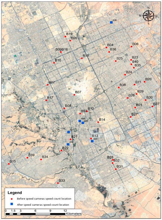
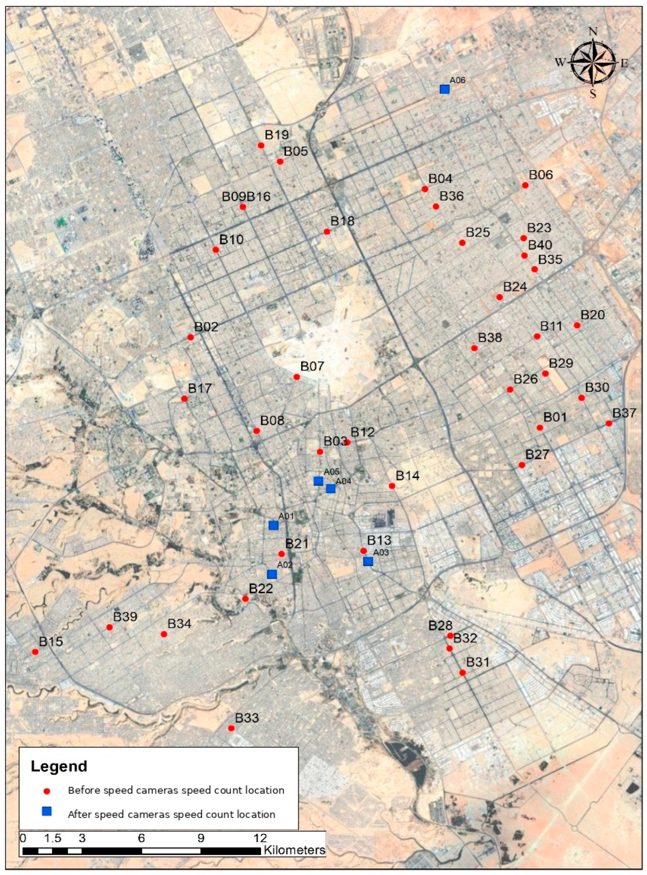
The study is situated on the urban road network of Riyadh, Saudi Arabia. Figure 1 shows the geographic configuration of the speed-count monitoring campaign. Red points labeled B01–B40 represent spatial before-camera count locations (before/upstream of the camera position), while blue points labeled A01–A06 represent spatial after-camera count locations (after/downstream of the camera position). Thus, B and A describe locations relative to a camera and are not temporal labels for data collected before versus after installation. The network spans central, northern, eastern, southern, and western sectors of Riyadh, although the current analysis uses only the five B-labeled sites for which classified records were available.
Figure 1.
Riyadh speed-count monitoring network.
The five analyzed sensor stations correspond to mapped locations B01, B05, B12, B26, and B27. They are the complete set of sites present in the classified speed-frequency dataset available for the 21–27 December 2025 analysis period; no classified records for the remaining mapped B sites or for A sites were available in that dataset. The subset is therefore availability-based rather than probability-sampled, and representativeness of the wider monitoring network is not assumed. To preserve continuity with the analytical station codes used throughout the data processing, the five sites are denoted B01–B05 in the statistical results, as mapped in Table 1. This distinction is important because the analytical code B02, for example, refers to mapped sensor B05 rather than map label B02.
Table 1.
Mapping between analytical station codes and Riyadh network sensor labels.
2.2. Observation Design and Traffic Classification
The observation period covers seven consecutive days, from 21 to 27 December 2025. Observations for each sensor direction were summarized in 24 one-hour periods per day. Vehicles were classified into eight categories: cars, motorcycles, minibusses, big buses, light commercial vehicles/pick-ups (LCV/pick-up), light trucks, medium trucks, and heavy trucks. Speed frequencies were stored in 15 consecutive 10 km/h bins spanning 10–160 km/h, represented analytically by bin midpoints from 15 to 155 km/h. The posted speed limit associated with the analyzed observations was 80 km/h.
The full dataset contains 2,310,276 vehicle passages. The regular design yields a maximum of 5 sites × 2 directions × 7 days × 24 h × 8 vehicle classes = 13,440 hourly class cells, of which 10,492 contain at least one vehicle and enter the multivariable mean-speed model. The study design and analytical dimensions are summarized in Table 2.
Table 2.
Study design and analytical dimensions.
2.3. Quality Control and Grouped-Data Preprocessing
The sensor frequency tables were checked for structural balance, valid direction/day/hour coding, nonnegative frequencies, consistent class labels, and a common speed-bin definition. Aggregation was performed by summing vehicle frequencies within the required site, class, day, direction, or hourly grouping. Because individual vehicle speeds were not retained, all mean and variance calculations use speed-bin midpoints. Percentile calculations use linear interpolation within the bin containing the target cumulative probability. This approach retains more information than assigning the percentile directly to a bin midpoint while remaining transparent about the resolution imposed by 10 km/h grouping.
Because the retained source provides grouped frequencies rather than individual vehicle speeds, a direct empirical comparison between interpolated and raw, unbinned V85 values cannot be performed. The 10 km/h binning therefore sets the intrinsic within-bin resolution of the percentile estimate. As a sensitivity check, assigning the 85th percentile to the midpoint of its containing bin instead of linearly interpolating changes the network V85 from 82.21 to 85.00 km/h (+2.79 km/h) and the B03 V85 from 86.97 to 85.00 km/h (−1.97 km/h). More generally, the unbinned percentile is identifiable from the available data only within the boundaries of its containing 10 km/h bin; interpolated V85/V95 values are therefore treated as grouped-data estimates rather than exact sub-bin measurements.
2.4. Governing Equations for Grouped Speed Distributions
Let be the number of vehicles in analysis group and speed bin , the midpoint of bin , and the number of speed bins. Total traffic volume is
The frequency-weighted mean speed is
Grouped standard deviation and coefficient of variation are calculated as
For percentile fraction , let denote the first bin for which the cumulative frequency reaches , the lower boundary of that bin, the cumulative frequency below it, its frequency, and km/h the bin width. The grouped percentile is estimated by
Equation (4) is used for , , and . Let km/h be the posted speed limit and the lower boundary of bin . Because exact within-bin speeds are unavailable, the bin-based exceedance probability is defined conservatively as
A normalized squared-speed exposure index (SEI) is used as a supplementary descriptor of the concentration of higher speeds:
The SEI is not a crash-risk model; it is a dimensionless speed-magnitude indicator motivated by the quadratic dependence of kinetic energy on speed.
Equations (1)–(6) form the common computational layer used to convert the 10 km/h grouped sensor frequencies into the indicators analyzed throughout the paper, rather than representing separate theoretical models. Equation (1) provides the total number of vehicle passages in each group and the frequency weights used in subsequent summaries; Equation (2) produces the mean speeds reported by class, site, day, direction, and hour and supplies the hourly response used in the regression and harmonic analyses; Equation (3) provides SD and CV to quantify dispersion and identify unusually heterogeneous locations; Equation (4) yields V50, V85, and V95 for central and upper-tail characterization; Equation (5) quantifies the share of observations in speed bins at or above the posted limit; and Equation (6) provides a supplementary normalized indicator of high-speed concentration. Applied consistently across all aggregation levels, these formulations transform the binned counts into directly comparable measures of exposure, central tendency, dispersion, percentile behavior, and compliance that underpin the later spatial, temporal, regression, and mixture-model interpretations.
2.5. Frequency-Weighted Fixed-Effects Harmonic Regression
To estimate adjusted differences in hourly mean speed, the 15 speed bins were first collapsed into one mean speed for each nonempty combination of vehicle class , site-direction , day , and hour . The model is
Cars, analytical station B01 in its reference direction, and Sunday are reference categories. Each hourly class cell is weighted by its vehicle count , so parameter estimates minimize
Coefficient uncertainty is estimated using two-way cluster-robust covariance with finite-cluster correction. The first clustering dimension is site-direction × calendar day (70 clusters), allowing arbitrary dependence among vehicle classes and hours observed within the same site–direction–day; the second is calendar day × hour (168 clusters), allowing common contemporaneous shocks across sites and vehicle classes. This robustness specification addresses within-site and temporal dependence that HC3 heteroskedasticity-only standard errors do not capture [25]. Harmonic amplitude and phase are summarized by Equation (9).
The fixed-effects model is descriptive and associational. It adjusts for observed categorical and cyclic factors but does not identify causal effects of road geometry, enforcement, or vehicle type. Cluster-robust covariance improves uncertainty estimation, but the independent spatial replication remains limited to five sites (ten site-directions) observed over seven calendar days.
2.6. Network-Level Harmonic Model Selection and Validation
A separate cyclic model was fitted to the 24 network-wide hourly mean speeds to evaluate how many harmonics are needed to reproduce the daily operating-speed curve. Candidate models with take the form
Model order was assessed using , root mean square error (RMSE), corrected Akaike information criterion (AICc), and leave-one-hour-out RMSE. AICc was given primary weight because it explicitly penalizes unnecessary complexity in the small 24-observation aggregate series.
2.7. Finite Gaussian Mixture Model for Latent Traffic Regimes
Site-level speed distributions were further modeled using finite Gaussian mixtures. For latent regimes, the speed density is
Parameters were estimated by frequency-weighted expectation maximization using the speed-bin midpoints. The grouped log-likelihood and Bayesian information criterion are
where is the number of free mixture parameters. To quantify how clearly two regimes are separated, the standardized component separation index is
Values of substantially above 2 indicate strongly separated latent components rather than a mild correction for skewness. As an additional robustness check focused on analytical station B03 (mapped B12), the mixture was re-estimated using a bin-integrated grouped likelihood and the integrated completed likelihood (ICL) criterion [26], separately for northbound and southbound traffic and for four broad time bands (00:00–05:00, 06:00–11:00, 12:00–17:00, and 18:00–23:00). This check avoids treating all observations in a 10 km/h bin as if they occurred exactly at the midpoint and directly tests whether directional or temporal pooling creates the apparent bimodality.
3. Results
3.1. Traffic Composition and Network-Wide Distribution
The sensor observations contain 2,310,276 vehicle passages. Cars account for 1,965,452 passages (85.07%), followed by LCV/pick-up vehicles (5.95%), minibusses (5.03%), light trucks (2.71%), motorcycles (0.75%), heavy trucks (0.23%), big buses (0.19%), and medium trucks (0.07%). The network-wide grouped mean speed is 63.24 km/h, approximately 16.8 km/h below the posted limit. In contrast, the grouped V85 is 82.21 km/h, so the upper tail crosses the 80 km/h limit even though the mean does not.
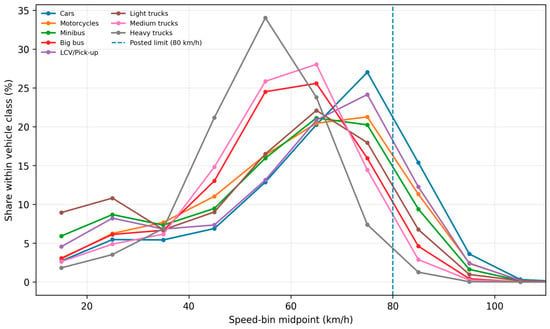
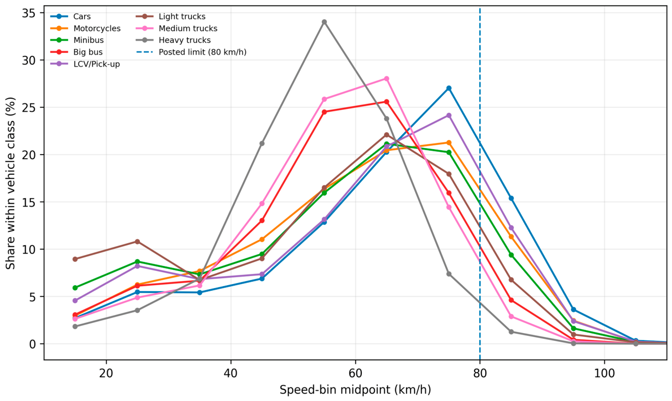
Figure 2 presents normalized speed distributions by vehicle class. Cars are concentrated predominantly in the 65–85 km/h range, while the distributions of buses and trucks shift toward lower speed bands. The figure also shows that differences between vehicle classes concern both location and spread rather than a simple uniform shift.
Figure 2.
Normalized vehicle-class speed distributions. The dashed vertical line marks the 80 km/h posted speed limit.
3.2. Vehicle-Class Speed Characteristics
Table 3 summarizes the principal class-level indicators. Cars have the highest mean speed (64.16 km/h) and V85 (82.81 km/h), with 19.32% of vehicles in bins beginning at or above 80 km/h. Motorcycles and LCV/pick-up vehicles also have relatively high upper tails, with V85 values of 79.50 and 79.95 km/h, respectively. Heavy trucks have the lowest V85 (67.35 km/h) and lowest estimated exceedance rate (1.30%).
Table 3.
Vehicle-class descriptive speed statistics.
The class-level contrast between central and upper-tail behavior is evident directly from Table 3. All vehicle-class means remain below the 80 km/h posted limit, whereas the car-class V85 exceeds it. These results reinforce the need to retain both central-tendency and upper-percentile indicators in class-specific speed management assessments.
3.3. Spatial and Directional Heterogeneity
Site-level differences are substantially larger than class-level differences. Table 4 shows that analytical station B04 has the highest mean speed (69.53 km/h), while B03 has the highest V85 (86.97 km/h), highest standard deviation (26.68 km/h), highest coefficient of variation (0.452), and highest estimated exceedance share (30.40%). B05 has the lowest mean speed (50.00 km/h) and contains no observations in bins beginning at 80 km/h or above.
Table 4.
Site-level speed distribution and compliance metrics.
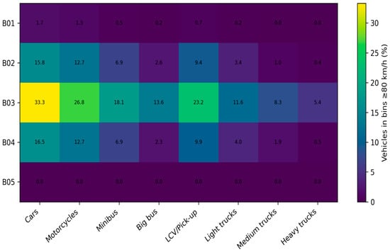
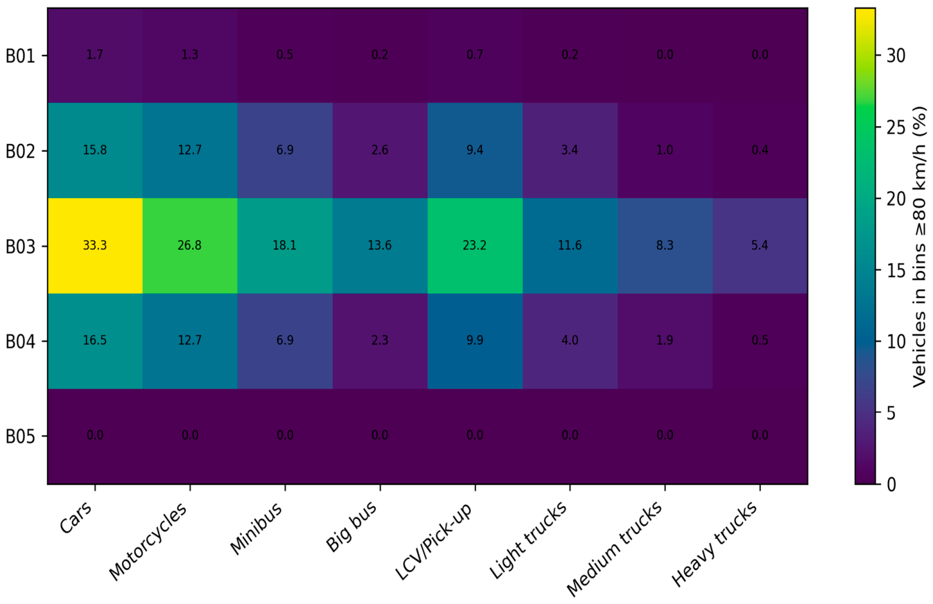
The site-by-vehicle-class exceedance matrix in Figure 3 demonstrates that the B03 anomaly is not confined to cars. B03 records the highest exceedance share for every vehicle class, including 33.3% for cars, 26.8% for motorcycles, 23.2% for LCV/pick-up vehicles, and 5.4% for heavy trucks. This consistency indicates a strong location effect superimposed on vehicle-class behavior.
Figure 3.
Percentage of vehicles in bins beginning at or above 80 km/h by analytical site and vehicle class.
Direction-specific aggregation further isolates the B03 pattern. B03 northbound has a mean speed of 52.17 km/h, V85 of 85.03 km/h, and 23.7% exceedance, whereas B03 southbound has a mean speed of 64.73 km/h, V85 of 88.02 km/h, and a substantially larger high-speed component. Thus, the site combines both directional asymmetry and within-direction dispersion.
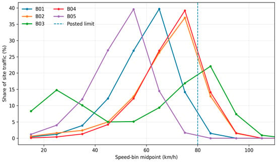
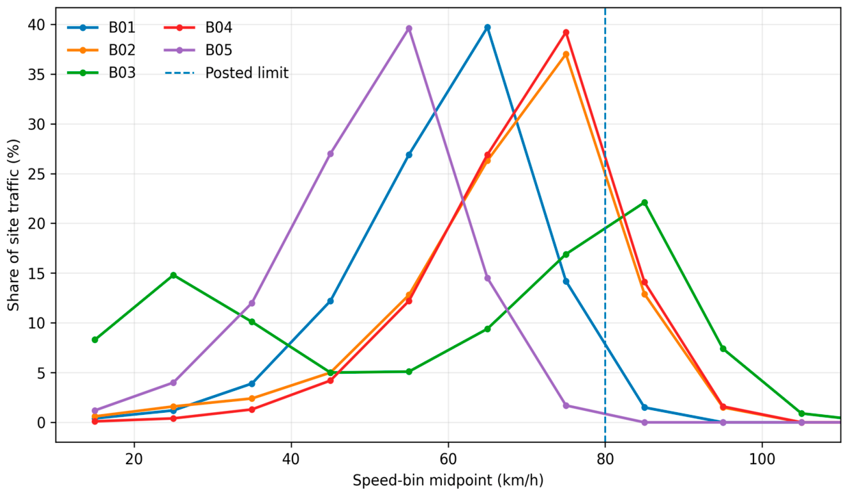
Figure 4 plots the complete site-level distributions. B01, B02, B04, and B05 are comparatively concentrated around a dominant operating range. Analytical station B03 exhibits the widest and most clearly multimodal distribution. It is qualitatively different, with one concentration at low speeds and another at approximately 75–95 km/h. This visual pattern motivates the mixture-model analysis in Section 3.7.
Figure 4.
Site-level speed distributions for all vehicle classes combined.
3.4. Diurnal and Day-of-Week Variation
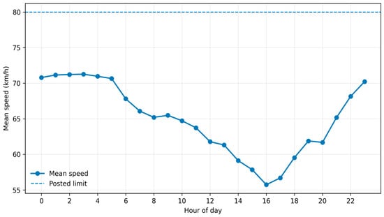
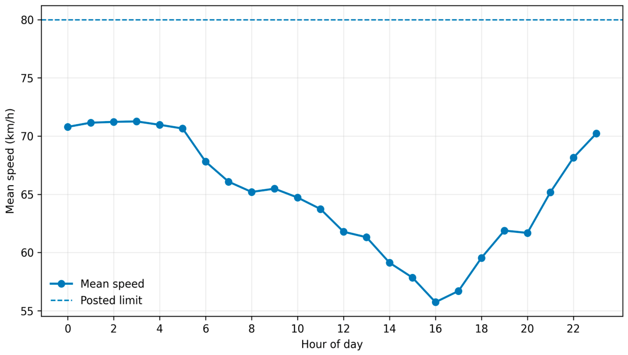
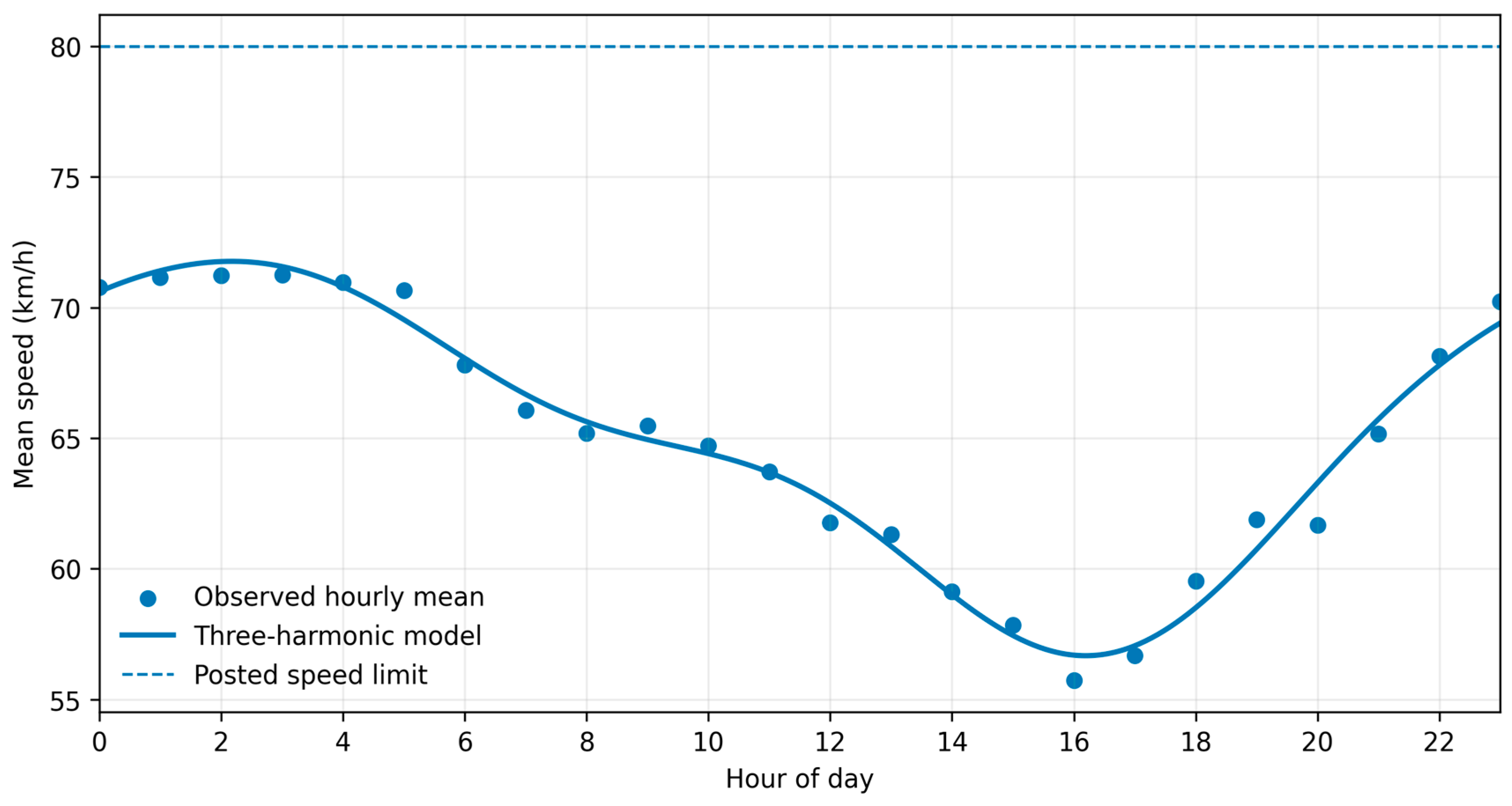
The network-wide hourly mean speed exceeds 70 km/h during much of the period from midnight to 05:00, and declines as daytime activity increases. The observed minimum occurs near 16:00 at 55.73 km/h, after which the speed recovers through the evening. Figure 5 illustrates this pronounced daily cycle.
Figure 5.
Network-wide hourly mean speed across the 24 h day.
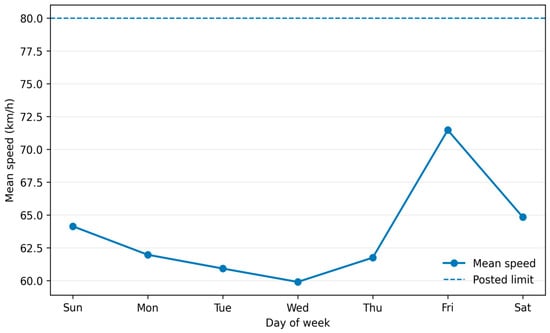
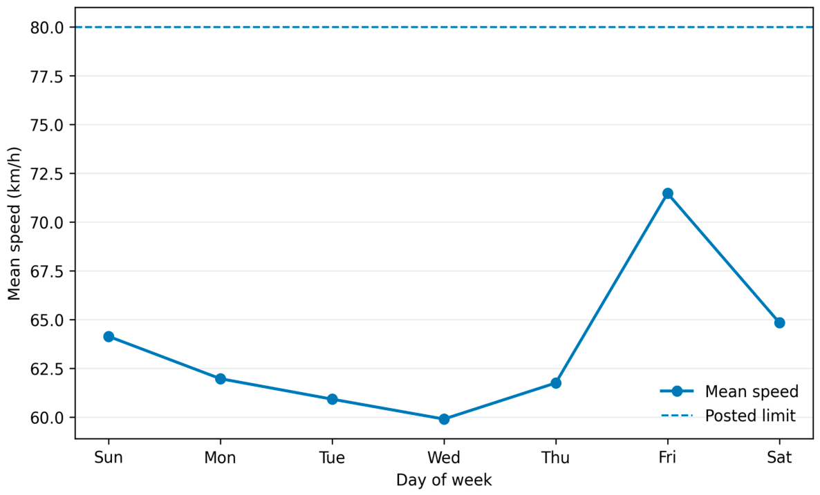
Day-of-week variation is also substantial (Figure 6). Friday has the lowest daily volume (262,411 passages) but the highest mean speed (71.47 km/h), V85 (86.09 km/h), and estimated exceedance rate (28.20%). Wednesday has the lowest mean speed at 59.90 km/h. The combination of lower Friday demand and higher operating speed is consistent with a traffic-state mechanism in which reduced interference allows a larger fraction of drivers to approach their desired speed.
Figure 6.
Day-of-week variation in network-wide mean speed.
3.5. Multivariable Weighted Fixed-Effects Model
The weighted fixed-effects harmonic model in Equation (7) was fitted to 10,492 nonempty hourly vehicle-class cells and achieved R2 = 0.353. Two-way cluster-robust covariance accounts for repeated observations within site–direction–day blocks and common day–hour shocks without changing the coefficient estimates. The moderate explanatory power is reasonable for grouped urban speed data because detailed geometry, signal timing, access density, incidents, and lane-level traffic state are not included.
All non-car classes have lower adjusted hourly mean speeds than cars, as shown in Table 5. Heavy trucks show the largest adjusted difference (−15.17 km/h; two-way cluster-robust 95% CI: −16.65 to −13.69), followed by medium trucks (−10.71 km/h) and light trucks (−7.93 km/h). Motorcycles are closest to cars, with an adjusted difference of −1.84 km/h (95% CI: −2.50 to −1.19). The substantive class contrasts therefore remain evident after accounting for clustered dependence. Complete coefficient-level results for the same model—including the intercept, all site-direction and day contrasts, and both harmonic pairs—are provided in Supplementary Table S1.
Table 5.
Vehicle-class coefficients from the frequency-weighted harmonic fixed-effects model. Standard errors and confidence intervals use two-way clustering by site-direction × calendar day and calendar day × hour.
Spatial effects remain large after class adjustment. Relative to B01 in the reference direction, the largest positive adjusted effects occur at B04 eastbound (+9.14 km/h), B04 westbound (+9.01 km/h), and B02 northbound (+8.20 km/h). B05 is approximately 9.3–9.5 km/h lower than the B01 reference. B03 remains strongly direction-dependent: the northbound effect is −8.18 km/h, whereas the southbound effect is +4.86 km/h. Friday is +7.28 km/h relative to Sunday after adjustment, while Wednesday is −4.28 km/h. The first daily harmonic has an amplitude of approximately 6.16 km/h and places the primary fitted maximum near 03:40, while the second harmonic improves representation of the afternoon trough and evening recovery. With two-way cluster-robust covariance, uncertainty for the day and site-direction contrasts is wider than suggested by heteroskedasticity-only inference; these coefficients are therefore interpreted as descriptive adjusted contrasts rather than precise causal or recurring weekday effects.
3.6. Harmonic Model Order and Diurnal Prediction
Table 6 compares candidate network-level harmonic orders. A single harmonic already explains 91.5% of the variation in the 24 hourly means, confirming that the dominant pattern is strongly cyclic. Adding a second harmonic raises to 0.974 and reduces RMSE. The three-harmonic model has the smallest AICc (1.77), with , RMSE = 0.670 km/h, and leave-one-hour-out RMSE = 0.946 km/h. A fourth harmonic increases complexity without improving predictive performance. A five-harmonic model achieves a lower leave-one-hour-out error but has a larger AICc than the three-harmonic solution; the three-harmonic model was therefore retained as the preferred balance between fidelity and parsimony.
Table 6.
Network-level harmonic model selection.
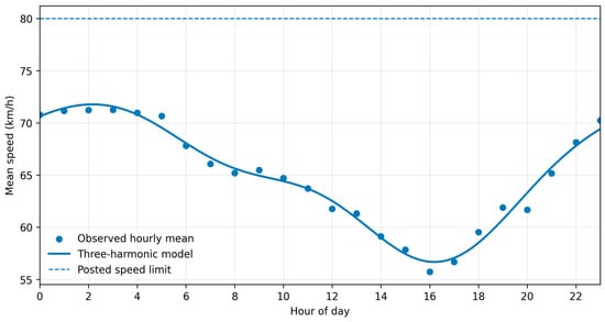
Figure 7 compares observed hourly means with the selected three-harmonic model. The fitted maximum is approximately 71.77 km/h at 02:10, and the fitted minimum is approximately 56.67 km/h at 16:12. The model reproduces the rapid morning decline, afternoon minimum, and evening recovery without discontinuity at midnight.
Figure 7.
Observed hourly network mean speeds and the selected three-harmonic cyclic model.
3.7. Gaussian Mixture Modeling of Site-Level Operating Regimes
Two-component Gaussian mixtures yield lower BIC values than a single Gaussian at every site, reflecting some degree of skewness or multi-regime operation in large urban samples. However, the strength and interpretation of the improvement differ substantially by site. Table 7 reports the two-component parameters and component separation index.
Table 7.
Two-component Gaussian mixture results for site-level grouped speed distributions.
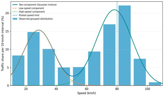
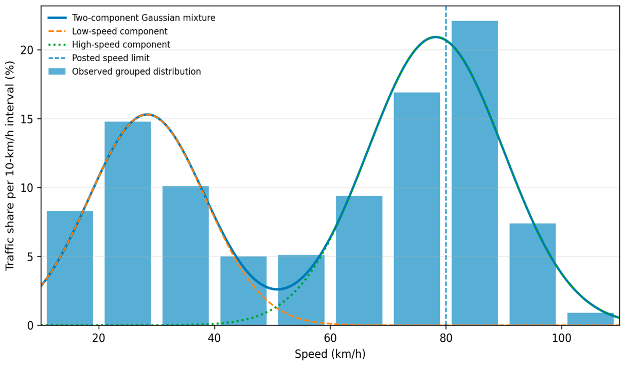
The most important finding concerns B03. Its estimated low-speed component contains 38.4% of traffic and is centered at 28.37 km/h, while the high-speed component contains 61.6% and is centered at 78.24 km/h. The standardized separation is far larger than at any other site and indicates two clearly distinct operating regimes rather than mild skewness. The two-component model reduces BIC by approximately 404,000 relative to a single Gaussian. A three-component sensitivity model further subdivides B03 into components centered near 25.5, 58.7, and 82.3 km/h; however, the two-component model is retained because it provides the clearest operational interpretation of a low-speed regime and a high-speed regime.
Figure 8 overlays the two-component mixture on the observed B03 speed distribution. The model confirms that the site mean of approximately 59 km/h lies between two substantial traffic states and therefore does not represent a typical vehicle as well as the regime-specific parameters do.
Figure 8.
Two-component Gaussian mixture representation of the B03 grouped speed distribution.
The additional stratified robustness analysis indicates that the B03 pattern is not solely an artifact of pooling directions. Under the bin-integrated/ICL specification, the site-level components are centered near 26.8 and 79.6 km/h (D = 4.08). Two components are also preferred within B03 northbound, with centers near 25.5 and 78.9 km/h (D = 4.51), and within B03 southbound, with centers near 30.1 and 80.3 km/h (D = 3.37). By time band, two components are supported during 06:00–23:00, whereas 00:00–05:00 is adequately represented by a single component. Thus, directional pooling alone is insufficient to explain the bimodality, although time-of-day composition contributes and the latent-regime interpretation is not invariant across all periods.
4. Discussion
4.1. Mean Speed Versus Upper-Tail Behavior
The central empirical result is the divergence between mean speed and upper-tail behavior. At the network level, the mean is 16.76 km/h below the posted limit, yet V85 exceeds the limit by 2.21 km/h. A management system based only on the mean would therefore classify the network as broadly compliant while missing a substantial high-speed subpopulation. The same issue appears more strongly at B03, where a mean near 59 km/h coexists with V85 near 87 km/h and an estimated 30.4% of vehicles in bins beginning at or above the limit.
This finding is consistent with both the established literature and the recent literature emphasizing that speed distributions should not be reduced to a single central measure [5,6,7,10,11,12,13,14]. From a safety management standpoint, V85 and exceedance share are valuable because they describe how much traffic is operating near or beyond the enforcement threshold. From a traffic-flow standpoint, dispersion and multimodality show whether the observed average results from a single operating state or from mixing qualitatively different regimes.
4.2. Interpretation of the B03 Latent Regimes
The Gaussian mixture results show that B03 operates differently from the other observed sites, although the available data limit the physical interpretation of its components. The main pooled fit contains a low-speed component near 28 km/h and a high-speed component near 78 km/h. The stratified sensitivity analysis shows that well-separated components persist within both northbound and southbound data, so simple directional pooling is not sufficient to explain the pattern. However, the 00:00–05:00 time band is adequately described by one component, indicating that time-of-day composition contributes to the pooled distribution. Because the available data do not include roadway geometry, signal status, lane occupancy, incidents, weather, or detector calibration metadata, the components are interpreted as statistical regimes rather than uniquely as congestion and free-flow states.
Accordingly, the lower-speed component should not be attributed uniquely to congestion or traffic signals. Plausible alternatives include a mixture of main-lane and service-road traffic, merging/diverging activity, access-related slowing, or other local geometric and traffic-control effects. Because lane configuration, detector field of view, signal timing, and queue data are unavailable, the present analysis cannot distinguish among these mechanisms.
This illustrates the value of mixture modeling as a descriptive diagnostic while also showing why stratification is needed before assigning operational meaning to the components. Park et al. [10] showed that mixture models can recover heterogeneity concealed by a single distribution; here, the persistence of separation within each direction strengthens the statistical evidence for B03 heterogeneity, while the time-band result prevents overstatement. B03 should therefore receive priority for detector verification and collection of geometry, control, queueing, traffic-state, and lane-level information before any specific mechanism or intervention is inferred.
4.3. Vehicle-Class Effects After Adjustment
The descriptive and adjusted analyses agree that vehicle class matters. Cars define the upper edge of the operating-speed distribution, while buses and trucks are slower after controlling for location, direction, day, and time. The adjusted heavy-truck difference of −15.17 km/h relative to cars remains large under two-way clustered uncertainty. These coefficients are pooled adjusted contrasts for the observed five-site dataset, not invariant class effects at every site or traffic state, and the model does not establish a causal effect of vehicle type.
The practical implication is that the same corridor can have different compliance profiles by class. A future camera–effect comparison—whether spatial B versus A or temporal pre-/post-installation—should therefore stratify by vehicle class or adjust explicitly for class shares, especially when traffic composition differs between compared observations.
4.4. Cyclic Temporal Structure and Low-Demand Speeding
The harmonic models show that time of day is strongly associated with operating speed. The selected three-harmonic model explains 98.1% of variation in the 24 network hourly means and identifies a nighttime/early-morning maximum and late-afternoon minimum. This pattern is consistent with greater freedom to select speed during low-demand conditions and reduced speeds when urban interactions intensify.
Beyond descriptive interpretation, the selected three-harmonic curve has a practical traffic-flow modeling role because it replaces 24 disconnected hourly means with a smooth, parsimonious 24 h speed profile. At the macroscopic level, this profile can be used as a time-varying speed benchmark or input for corridor/network simulation, dynamic traffic assignment, performance monitoring, and time-dependent control or enforcement scheduling. At the microscopic level, it can provide the time-of-day reference mean for calibrating desired speed distributions, while the observed vehicle-class and site-specific dispersion and mixture results characterize heterogeneity around that reference. Such use requires local calibration and validation; the harmonic curve is a temporal speed representation, not a stand-alone car-following or traffic-flow law.
Friday reinforces the observed week-specific low-demand/high-speed pattern, but the dataset contains only one occurrence of each weekday. Accordingly, these day coefficients are treated as date-specific descriptive contrasts rather than recurring weekday effects. If a temporal pre-/post-installation camera evaluation is pursued, observations should be matched or adjusted by calendar day and hour, with repeated weeks or seasons used to distinguish intervention effects from normal temporal variability.
4.5. Implications for Automated Speed-Enforcement Evaluation in Riyadh
The network map contains B- and A-labeled monitoring locations that are spatially defined relative to camera positions. The present dataset, however, contains only five B-labeled sites for one week and includes neither the corresponding A-site records required for a spatial upstream/downstream comparison nor a temporal pre-/post-installation intervention contrast. No causal statement about camera installation or camera effectiveness should therefore be drawn from the current analysis.
Future evaluation should first specify the intended contrast. If B and A are compared as spatial positions around an existing camera, the analysis should use matched upstream/downstream observations while accounting for camera distance, direction, roadway geometry, traffic state, day, hour, and vehicle class; this is not a temporal before–after design. If installation or activation dates and untreated comparison sites become available, a separate temporal pre-/post design—potentially including a controlled before–after or difference-in-differences model—could be considered after its identifying assumptions are assessed [27,28]. In either case, distributional outcomes such as mean speed, V85, V95, exceedance measures, and mixture structure should be evaluated rather than mean speed alone.
Saudi evidence already suggests that automated enforcement can influence traffic-related outcomes and driver compliance [17,18,19,20,21]. The contribution of the present study is therefore an empirical and integrative five-site baseline rather than a new or high-resolution statistical framework. Its value lies in applying established distributional summaries, passage-weighted fixed effects with cluster-robust inference, cyclic modeling, and mixture diagnostics together, while making the sampling scope and the distinction between spatial B/A labels and any future temporal intervention design explicit.
4.6. Engineering and Policy Implications
The results support a targeted rather than uniform speed management strategy. B03 should be prioritized because it combines the highest V85, greatest dispersion, largest exceedance share, strongest directional asymmetry, and most distinct multimodality. B04 and B02 also warrant attention because of relatively high mean speed and V85. B05, by contrast, is unlikely to be a speeding priority during the observed week, although low speeds may indicate operational constraints that deserve separate congestion analysis.
Temporal targeting is equally important. Overnight and early-morning periods have the highest fitted speeds, and Friday has the highest daily exceedance. Enforcement scheduling, dynamic warnings, and corridor monitoring can therefore be directed toward periods with greater observed high-speed exposure. Such targeting should be combined with site-specific engineering review rather than interpreted as a substitute for geometric or traffic-control improvements.
5. Limitations
Several limitations guide interpretation. First, speed is available in 10 km/h bins rather than as individual measurements, so midpoint-based means and standard deviations are approximations, and the exceedance measure in Equation (5) is bin-based. Second, the analyzed week is a single seven-day period in December 2025; seasonal, repeated-weekday, weather, event, and incident effects are not represented. Third, only five of the mapped B-labeled monitoring sites are present in the supplied classified dataset. They form an availability-based, non-probability subset and have not been shown to be representative of the wider Riyadh network; pooled findings should therefore not be generalized citywide. Fourth, roadway geometry, lane count, signal timing, access density, traffic density/occupancy, incidents, weather, camera distance, and detector calibration information are unavailable, limiting mechanistic interpretation of site effects and the B03 mixture structure. Fifth, the fixed-effects model is associational. Two-way cluster-robust covariance addresses important within-site-day and common time dependence, but the number of independent sites remains small and clustered inference does not create causal identification. Sixth, the Gaussian mixture model identifies statistical regimes; the direction- and time-stratified checks reduce concern about simple pooling artifacts but do not prove that a component uniquely represents congestion or free flow. Finally, B/A are spatial camera-relative labels, and the current dataset contains no A-site records and no temporal pre-/post-installation panel; consequently, the study does not estimate the causal effect of speed camera deployment.
In addition, the grouped-data structure prevents direct estimation of the bias of interpolated V85/V95 relative to raw vehicle-level percentiles; the sensitivity check in Section 2.3 should therefore be interpreted as a resolution check rather than a validation against unbinned data. The single December week also does not capture Riyadh’s extreme summer conditions or altered travel patterns during school and public holidays and other seasonal periods; annual generalization requires repeated multi-season observations.
6. Conclusions and Recommendations
This study provides an exploratory baseline assessment of operating-speed behavior at five Riyadh monitoring locations using 2,310,276 classified vehicle passages recorded over 21–27 December 2025. The principal conclusions are restricted to these sites and this observation period:
- The pooled mean speed was 63.24 km/h, whereas V85 was 82.21 km/h under an 80 km/h limit. Thus, a mean 16.76 km/h below the limit coexisted with an upper percentile 2.21 km/h above it. Monitoring should retain percentile and bin-based exceedance measures alongside the mean to identify high-speed exposure.
- Cars accounted for 85.07% of all passages and had the highest class-level mean speed (64.16 km/h) and V85 (82.81 km/h); 19.32% were in speed bins beginning at or above 80 km/h. Heavy trucks had a V85 of 67.35 km/h and a corresponding share of 1.30%. These contrasts support vehicle-class-specific monitoring and adjustment for traffic composition when comparing sites or periods.
- Site rankings depended on the indicator used. B04 had the highest mean speed (69.53 km/h), but B03 combined a lower mean (59.06 km/h) with the highest V85 (86.97 km/h), SD (26.68 km/h), CV (0.452), and bin-based exceedance share (30.40%). B05 had a mean of 50.00 km/h and no observations in bins beginning at or above 80 km/h. B03 therefore warrants priority for detector verification and site investigation before a specific intervention is selected.
- The weighted fixed-effects model explained 35.3% of variation in hourly class-cell mean speeds. Heavy trucks were 15.17 km/h slower than cars after adjustment (two-way cluster-robust 95% CI: −16.65 to −13.69 km/h), while motorcycles were 1.84 km/h slower (95% CI: −2.50 to −1.19 km/h). These pooled associations show that class differences remain after accounting for site-direction, day, and cyclic time-of-day variation.
- The selected three-harmonic model explained 98.1% of variation in the 24 aggregated hourly mean speeds, with RMSE = 0.670 km/h, leave-one-hour-out RMSE = 0.946 km/h, and the lowest AICc (1.77) among the candidate orders. Its fitted maximum was 71.77 km/h near 02:10, and its minimum was 56.67 km/h near 16:12. The resulting continuous profile provides a compact temporal benchmark, subject to validation on additional observation periods.
- Friday combined the lowest daily volume (262,411 passages) with the highest daily mean speed (71.47 km/h) and bin-based exceedance share (28.20%). Together with the overnight speed maximum, this finding identifies lower-demand periods as priorities for further monitoring; repeated weeks are needed to establish whether the Friday pattern recurs.
- At B03, the two-component mixture assigned 38.4% of traffic to a component centered at 28.37 km/h and 61.6% to one centered at 78.24 km/h, with strong standardized separation (D = 4.57). Bin-integrated sensitivity analysis retained two components within each direction and during 06:00–23:00, whereas one component was sufficient during 00:00–05:00. The pooled mean therefore conceals distinct statistical regimes whose physical causes require additional field information.
- The B and A labels describe monitoring positions upstream and downstream of cameras. Because the present records contain only five B sites, they provide a baseline and do not estimate camera effectiveness. Future evaluation must specify a spatial upstream/downstream or temporal pre-/post-installation comparison and collect the corresponding comparison observations and covariates.
For practice, monitoring should prioritize B03 for field and detector checks, with additional attention to B04 and B02, and retain upper-tail indicators by vehicle class, direction, and time of day. After local calibration and validation, the harmonic profile can provide a time-varying benchmark for corridor or network simulation, while the class-specific dispersion and mixture parameters can inform desired speed distributions. Repeated monitoring can then assess whether engineering measures, including appropriate traffic-calming designs, and enforcement interventions reduce high-speed exposure. Such evaluations should use comparable observation periods and explicitly defined comparison groups.
Supplementary Materials
The following supporting information can be downloaded at https://www.mdpi.com/article/10.3390/vehicles8100231/s1. Table S1: Full coefficient results from the frequency-weighted harmonic fixed-effects model.
Author Contributions
Conceptualization, M.O., A.S.A. and M.A.E.S.; methodology, M.O. and M.A.E.S.; software, M.O.; validation, M.O., A.S.A. and M.A.E.S.; formal analysis, M.O.; investigation, M.O., A.S.A. and M.A.E.S.; resources, A.S.A. and M.A.E.S.; data curation, M.O. and A.S.A.; writing—original draft preparation, M.O.; writing—review and editing, M.O., A.S.A. and M.A.E.S.; visualization, M.O.; supervision, A.S.A. and M.A.E.S.; project administration, M.O.; funding acquisition, M.O., A.S.A. and M.A.E.S. All authors have read and agreed to the published version of the manuscript.
Funding
This research received no external funding.
Data Availability Statement
The data are available from the corresponding author upon reasonable request at maowais@aun.edu.eg.
Conflicts of Interest
The authors declare no conflict of interest.
Abbreviations
The following abbreviations and mathematical symbols are used in this manuscript:
| Abbreviation | Definition | |
| 1G | one-component Gaussian model | |
| 2G | two-component Gaussian mixture model | |
| A | after-camera count-location prefix; a spatial downstream label relative to a camera | |
| AICc | corrected Akaike information criterion | |
| B | before-camera count-location prefix; a spatial upstream label relative to a camera | |
| BIC | Bayesian information criterion | |
| CI | confidence interval | |
| CV | coefficient of variation | |
| HC3 | heteroskedasticity-consistent covariance matrix estimator, type 3 | |
| ICL | integrated completed likelihood criterion | |
| LCV | light commercial vehicle | |
| RMSE | root-mean-square error | |
| SD | standard deviation | |
| SE | standard error | |
| SEI | speed exposure index | |
| Mathematical symbols | ||
| Symbol | Definition | |
| indices for analysis group, speed bin, vehicle class, site-direction, day, and hour, respectively | ||
| number of speed bins | ||
| total vehicle count in analysis group g; vehicle count in group g and speed bin i | ||
| midpoint of speed bin i; lower boundary of speed bin i | ||
| frequency-weighted grouped mean speed, grouped standard deviation, and coefficient of variation for group g | ||
| percentile fraction in Equation (4) (also used locally for the number of free mixture parameters in Equation (12)); first bin whose cumulative frequency reaches the target percentile | ||
| lower boundary of percentile-containing bin j; cumulative frequency below bin j; frequency in bin j; speed-bin width (10 km/h) | ||
| grouped percentile speed for fraction p in group g; 50th-, 85th-, and 95th-percentile speeds | ||
| posted speed limit (80 km/h in this study) | ||
| bin-based probability/share of observations in group g at or above the posted speed limit | ||
| normalized squared-speed exposure index for group g | ||
| hourly mean speed and vehicle-count weight for vehicle class c, site-direction s, day d, and hour h | ||
| regression intercept; vehicle-class, site-direction, and day fixed effects | ||
| sine coefficient, cosine coefficient, and harmonic-order index for harmonic k | ||
| regression error term for cell c,s,d,h | ||
| frequency-weighted least-squares objective function over the regression-parameter vector | ||
| harmonic amplitude, harmonic phase, and phase-derived peak hour for harmonic k | ||
| network-wide mean speed at hour h; number of harmonics in the network-level cyclic model | ||
| generic speed variable; finite-mixture speed density | ||
| mixture weight for component k, with component weights summing to one | ||
| mean, standard deviation, and variance of Gaussian mixture component k | ||
| Gaussian density of speed for mixture component k | ||
| grouped frequency in speed bin i; total sample size used in the mixture-model information criterion | ||
| grouped log-likelihood; mixture-model parameter vector | ||
| normal density evaluated at the speed-bin midpoint for mixture component k | ||
| standardized component-separation index | ||
| adjusted speed difference in Table 5; BIC difference between the 1G and 2G models in Table 7 | ||
| coefficient of determination | ||
References
- Federal Highway Administration. Roundabouts. Proven Safety Countermeasures; FHWA-SA-21-042. Available online: https://highways.dot.gov/safety/proven-safety-countermeasures/roundabouts (accessed on 21 September 2026).
- Macioszek, E.; Tumminello, M.L. Simulating vehicle-to-vehicle communication at roundabouts. Transp. Probl. 2024, 19, 45–57. [Google Scholar] [CrossRef] [Scilit]
- Elvik, R. A re-parameterisation of the Power Model of the relationship between the speed of traffic and the number of accidents and accident victims. Accid. Anal. Prev. 2013, 50, 854–860. [Google Scholar] [CrossRef] [Scilit] [PubMed]
- Elvik, R.; Vadeby, A.; Hels, T.; van Schagen, I. Updated estimates of the relationship between speed and road safety at the aggregate and individual levels. Accid. Anal. Prev. 2019, 123, 114–122. [Google Scholar] [CrossRef] [Scilit] [PubMed]
- Dey, P.P.; Chandra, S.; Gangopadhaya, S. Speed distribution curves under mixed traffic conditions. J. Transp. Eng. 2006, 132, 475–481. [Google Scholar] [CrossRef] [Scilit]
- Hashim, I.H. Analysis of speed characteristics for rural two-lane roads: A field study from Minoufiya Governorate, Egypt. Ain Shams Eng. J. 2011, 2, 43–52. [Google Scholar] [CrossRef] [Scilit]
- Jun, J. Understanding the variability of speed distributions under mixed traffic conditions caused by holiday traffic. Transp. Res. Part C Emerg. Technol. 2010, 18, 599–610. [Google Scholar] [CrossRef] [Scilit]
- Federal Highway Administration. Traffic Monitoring Guide; U.S. Department of Transportation: Washington, DC, USA, 2016.
- Federal Highway Administration. Traffic Data Computation Method Pocket Guide; FHWA-PL-18-027; U.S. Department of Transportation: Washington, DC, USA, 2018.
- Park, B.-J.; Zhang, Y.; Lord, D. Bayesian mixture modeling approach to account for heterogeneity in speed data. Transp. Res. Part B Methodol. 2010, 44, 662–673. [Google Scholar] [CrossRef] [Scilit]
- Mondal, S.; Gupta, A. Speed distribution for interrupted flow facility under mixed traffic. Physica A Stat. Mech. Its Appl. 2021, 570, 125798. [Google Scholar] [CrossRef] [Scilit]
- Antwi, E.B.; Zhang, X.; Chen, M. Estimating Urban Arterial Traffic Speed Distributions Using XGBoostLSS. Transp. Res. Rec. 2024, 2678, 1811–1823. [Google Scholar] [CrossRef] [Scilit]
- Horbachov, P.; Minh, V.D.; Svichynskyi, S.; Liubyi, Y.; Muzylyov, D.; Ivanov, V. A study of vehicle speed distribution influenced by urban traffic conditions. Acta Logist. 2025, 12, 301–310. [Google Scholar] [CrossRef] [Scilit]
- Sarkar, D.R.; Kumar, P. An investigation of traffic speed distributions for uninterrupted flow at blackspot locations in a mixed traffic environment. IATSS Res. 2024, 48, 180–188. [Google Scholar] [CrossRef] [Scilit]
- Bar-Gera, H.; Schechtman, E.; Musicant, O. Evaluating the effect of enforcement on speed distributions using probe vehicle data. Transp. Res. Part F Traffic Psychol. Behav. 2017, 46, 271–283. [Google Scholar] [CrossRef] [Scilit]
- Graham, D.J.; Naik, C.; McCoy, E.J.; Li, H. Do speed cameras reduce road traffic collisions? PLoS ONE 2019, 14, e0221267. [Google Scholar] [CrossRef] [Scilit] [PubMed]
- Alobaidallah, A.M.; Alqahtany, A.; Maniruzzaman, K.M. Safety effectiveness of automated traffic enforcement systems: A critical analysis of existing challenges and solutions. Future Transp. 2025, 5, 25. [Google Scholar] [CrossRef] [Scilit]
- Abdulrahman, R.; Almoshaogeh, M.; Haider, H.; Alharbi, F.; Jamal, A. Development and application of a risk analysis methodology for road traffic accidents. Alex. Eng. J. 2025, 111, 293–305. [Google Scholar] [CrossRef] [Scilit]
- Alghnam, S.; Alkelya, M.; Alfraidy, M.; Al-bedah, K.; Tawfiq Albabtain, I.; Alshenqeety, O. Outcomes of road traffic injuries before and after the implementation of a camera ticketing system: A retrospective study from a large trauma center in Saudi Arabia. Ann. Saudi Med. 2017, 37, 1–9. [Google Scholar] [CrossRef] [Scilit] [PubMed]
- Alghnam, S.; Towhari, J.; Alkelya, M.; Binahmad, A.; Bell, T.M. The effectiveness of introducing detection cameras on compliance with mobile phone and seatbelt laws: A before-after study among drivers in Riyadh, Saudi Arabia. Inj. Epidemiol. 2018, 5, 31. [Google Scholar] [CrossRef] [Scilit] [PubMed]
- Alharbi, R.J. National trends in road traffic injuries and fatalities in Saudi Arabia from 2000 to 2023. Sci. Rep. 2025, 15, 42838. [Google Scholar] [CrossRef] [Scilit] [PubMed]
- Maghrour Zefreh, M.; Török, Á. Distribution of traffic speed in different traffic conditions: An empirical study in Budapest. Transport 2020, 35, 68–86. [Google Scholar] [CrossRef] [Scilit]
- Gao, C.; Xu, J.; Li, Q.; Yang, J. The effect of posted speed limit on the dispersion of traffic flow speed. Sustainability 2019, 11, 3594. [Google Scholar] [CrossRef] [Scilit]
- Saudi Highway Code. SHC 601–Traffic Engineering. Kingdom of Saudi Arabia; Current Edition. Available online: https://www.scribd.com/document/718393891/SHC-601-Final (accessed on 22 September 2026).
- Cameron, A.C.; Gelbach, J.B.; Miller, D.L. Robust inference with multiway clustering. J. Bus. Econ. Stat. 2011, 29, 238–249. [Google Scholar] [CrossRef] [Scilit]
- Biernacki, C.; Celeux, G.; Govaert, G. Assessing a mixture model for clustering with the integrated completed likelihood. IEEE Trans. Pattern Anal. Mach. Intell. 2000, 22, 719–725. [Google Scholar] [CrossRef] [Scilit]
- Owais, M. Traffic sensor location problem: Three decades of research. Expert Syst. Appl. 2022, 208, 118134. [Google Scholar] [CrossRef] [Scilit]
- Owais, M.; El Deeb, M.; Abbas, Y.A. Distributing Portable Excess Speed Detectors in AL Riyadh City. Int. J. Civ. Eng. 2020, 18, 1301–1314. [Google Scholar] [CrossRef] [Scilit]

Disclaimer/Publisher’s Note: The statements, opinions and data contained in all publications are solely those of the individual author(s) and contributor(s) and not of MDPI and/or the editor(s). MDPI and/or the editor(s) disclaim responsibility for any injury to people or property resulting from any ideas, methods, instructions or products referred to in the content. |
© 2026 by the authors. Licensee MDPI, Basel, Switzerland. This article is an open access article distributed under the terms and conditions of the Creative Commons Attribution (CC BY) license.