NSVD: Vehicle Image Dataset from Northern Slovakia Under Diverse Weather Conditions

Abstract

Existing vehicle detection models, typically trained on general-purpose or non-regional datasets, frequently underperform when applied to local traffic monitoring systems that rely on fixed roadside cameras. Changes in viewpoint, object size, local vehicle types and road conditions creates a domain mismatch between the training and target data. In addition, general datasets lack a dedicated class for van-bodied vehicles, despite their relevance to traffic monitoring. To address these limitations, we introduce the Northern Slovakia Vehicle Dataset (NSVD), specifically designed to capture European vehicle types. NSVD comprises nearly 8000 human-reviewed images collected from four fixed roadside sites in northern Slovakia and annotated with four visual weather conditions. We evaluate the transfer of You Only Look Once (YOLO) and Real-Time Detection Transformer (RT-DETR) models from general object detection to this roadside setting, and we introduce an evaluation protocol that accounts for the differing vehicle class definitions used in the source and target datasets. Training on NSVD improved detection across all evaluated classes and object sizes. The performance differences among the leading fine-tuned models were smaller than the improvement obtained from training on the target data. Results for individual weather conditions must be interpreted jointly with site and class composition, and they are therefore reported as descriptive findings. A leave-one-site-out evaluation shows that the impact of excluding a site from training ranges from minimal at one roadside location to substantial at the city-center site. NSVD provides a public benchmark for the development and transparent evaluation of vehicle detectors intended for fixed roadside cameras.

1. Introduction

Fixed roadside cameras provide continuous visual data for traffic monitoring. Vehicle detection is the first step in systems that track vehicles, estimate class-specific traffic flow, and support incident analysis [1,2]. Detection errors affect every later stage. An overall detection score can also hide poor results for a vehicle class that is important to a transport operator. A detector should therefore be evaluated using the viewpoint, vehicle types, and road conditions in which it will operate.

Images from roadside cameras differ from the images used to train most general object detectors. A roadside camera is fixed and usually observes the road from an elevated, oblique position. Vehicles are small at longer distances and can be partly hidden by other road users. Rain reduces contrast and creates reflections. Snow changes the background and can cover road markings. These effects appear together in real traffic video. Performance on a general benchmark does not show how well a detector will handle this setting.

Many vehicle-detection systems begin with a model trained on the Microsoft Common Objects in Context (MS COCO) dataset [3]. Frequently deployed architectures include the You Only Look Once (YOLO) framework [4,5] and Real-Time Detection Transformer (RT-DETR) models [6,7,8]. Previous studies have improved detection performance via image enhancement, changes to the detector and domain adaptation [9,10,11,12], and recent work continues in this direction with stronger backbones, super-resolution front ends, and multimodal fusion [13,14]. However, much of this work focuses on vehicle-mounted cameras or considers only a single type of image degradation. As a result, current findings offer limited insights into detector performance for fixed roadside cameras under dynamic, naturally changing conditions.

Applying a general detector to local roadside data creates two problems. The first is a change in image appearance. Viewpoint, background, object size, local vehicle types and weather conditions differ from the source data. The second is a difference in vehicle classes. MS COCO does not contain a separate van class. When a COCO detector is evaluated on a local traffic dataset, van-bodied vehicles must be ignored or assigned to another class. This choice changes both the score and its interpretation. The evaluation must therefore state how the source and target classes are matched.

Existing datasets cover individual aspects of this problem. Some provide images from fixed traffic cameras, while others include weather labels, detailed vehicle classes, or roadside sensor data. However, none of the datasets considered in this study combines fixed roadside images from Slovakia, balanced image counts across four weather conditions, a distinct visual van class, and a predefined benchmark split—features that are particularly important for capturing vehicle types commonly operating in Central Europe.

To address this gap, we introduce the Northern Slovakia Vehicle Dataset (NSVD). The images were recorded at four sites in the Žilina Region of northern Slovakia. This region lies near the borders with Poland and the Czech Republic and is traversed by major European routes (E50 and E75), resulting in a mix of local and international vehicle traffic from neighboring and other European countries. Every released bounding box was reviewed by expert annotators.

We use NSVD to measure the difference between general COCO checkpoints and models trained on the roadside data. We also compare several detector families using the same split, image size, number of epochs, and random seed. Performance is reported by vehicle class, object size, and visual weather label. The weather results describe the recorded subsets but do not isolate the effect of weather. The predefined split tests the same camera viewpoints that were used for training, so we also report a site-disjoint evaluation.

The main contributions are the following:

• We created and publicly released the NSVD dataset as the main contribution of this work. It contains vehicle annotations from four fixed roadside sites in northern Slovakia. Expert annotators reviewed all released boxes. The dataset has equal image counts for four visual weather labels and includes a predefined same-viewpoint benchmark split. The release also carries a per-image camera identifier, so that site-disjoint protocols can be defined on it.
• We define an evaluation protocol for the different class sets used by MS COCO and NSVD. The protocol states how van-bodied vehicles are handled and reports both common-class and full four-class results.
• We provide reference results for eleven YOLO and RT-DETR configurations trained under a common recipe. Four of them, covering both detector families, are repeated over three random seeds, and the spread across seeds is reported beside the benchmark. The remaining models are single runs. Results are given by class, object size, and visual weather label, each with the annotation count that supports it, together with model timing and a site-disjoint evaluation.

The remainder of the article is organized as follows. Section 2 reviews vehicle detectors and related roadside datasets. Section 3 describes the creation of NSVD, the evaluation protocols, and the training setup. Section 4 presents the experimental results. Section 5 discusses their meaning and limitations. Section 6 concludes the article.

2. Related Work

Because this study contributes a dataset and evaluation protocol rather than a new detector, we review both the model families and datasets relevant to fixed roadside vehicle detection.

2.1. Real-Time Detection Under Changing Conditions

One-stage detectors are widely used in traffic monitoring because they combine object localization and classification in a single model. The YOLO family is a common example [4,5]. Recent traffic applications have improved feature fusion and the detection of small objects [1,2]. The Detection Transformer (DETR) introduced end-to-end set prediction for object detection [6]. RT-DETR and D-FINE adapt this idea to efficient detection. D-FINE further improves localization through fine-grained distribution refinement [7,8,15]. These detector families use different prediction designs and cover a wide range of computational costs. They therefore provide useful reference models for the NSVD benchmark.

The benchmark includes several YOLO releases and model sizes. YOLO12 uses an attention-centered design, which means that the complete YOLO set is not purely convolutional [16]. RT-DETR provides an end-to-end transformer comparison. The purpose is to measure practical model configurations after training on NSVD. The experiment is not intended to establish that one detector family is generally better than another.

Weather and low visibility can change contrast, color, reflections, and object boundaries. One line of work improves the image before detection. Image-Adaptive YOLO (IA-YOLO) is an example of this approach [9]. A second line changes the detection network through attention, feature selection, or sensor fusion [10,17,18]. A third line of studies transfer between source and target domains [11,12,19,20]. These approaches address different problems. This study does not propose an image enhancement method, a weather-specific module, or an unsupervised adaptation method. It evaluates existing detectors before and after supervised training on labeled images from the target roadside sites.

Supervised training on the target data provides a direct measure of the benefit of labeled roadside images. Unsupervised domain adaptation assumes that target images are available without labels [11,19]. Domain generalization aims at a target domain that was not available during training [12]. NSVD does not evaluate either of these settings. The benchmark measures supervised fine-tuning and same-viewpoint testing. The release can still serve both, because the camera identifiers published with the dataset let individual cameras act as sources and target domains. An adaptation protocol may then use the unlabeled training images of a target camera but never its labels, whereas a generalization protocol must exclude that camera from training and validation entirely. The van mapping matters in either case: a target domain without a van category silently changes the label space.

2.2. Datasets and Vehicle Taxonomies

Driving datasets cover a range of tasks and viewpoints. KITTI, BDD100K, Cityscapes, Mapillary Vistas, nuScenes, ONCE, and the Waymo Open Dataset were recorded mainly from moving vehicles [21,22,23,24,25,26,27]. They provide broad road-scene coverage but do not represent the fixed camera geometry used in this study. The Vehicle Detection in Adverse Weather Nature (DAWN) dataset provides bounding boxes in fog, rain, snow, and sand [28]. The Adverse Conditions Dataset with Correspondences (ACDC) focuses on semantic understanding in adverse conditions [29]. Foggy Cityscapes provides synthetic fog applied to Cityscapes images rather than naturally recorded fixed-camera conditions [30]. The Nordic Vehicle Dataset studies vehicle detection in snowy scenes from an unmanned aerial vehicle [31]. These resources show the value of condition-specific data, although their viewpoints and label sets differ from NSVD.

Roadside datasets are closer to the present setting. UA-DETRAC and the MIOvision Traffic Camera Dataset (MIO-TCD) contains dense traffic-camera annotations [32,33]. UA-DETRAC also provides condition labels and the van class. MIO-TCD includes the work-van class. The Traffic Surveillance Benchmark for Occluded Vehicles under Various Weather Conditions (TSBOW) provides a recent fixed traffic-camera benchmark with rain, snow, haze, and normal scenes [34]. More recent infrastructure datasets such as Rope3D, DAIR-V2X, and the A9 Dataset support roadside three-dimensional perception and sensor fusion [35,36,37]. Their scale, viewpoints and sensing goals differ from the two-dimensional camera setting studied here. Fixed cameras, condition labels, and van categories already appeared in earlier datasets. NSVD combines these properties in a public Slovak roadside dataset. It also provides equal image counts across four visual weather labels and paired cross-taxonomy reporting. We therefore present NSVD as a setting-specific dataset rather than the first roadside or van-aware benchmark.

Small objects and degraded appearance are also studied elsewhere, for example, with super-resolution front ends on recent YOLO backbones in orchards [13] and camera–range fusion in railway scenes [14]. A single fixed roadside camera has no range channel, and its degradation comes from weather, so such methods still need labeled data from the setting in which they are meant to run.

Vehicle labels are not consistent across datasets. KITTI includes a van category, while MS COCO and BDD100K do not [3,21,22]. Even when two datasets use the same class name, their visual rules can differ. A score is therefore meaningful only when the mapping between source predictions and target annotations is stated. NSVD addresses this issue with two protocols. One uses the populated classes shared with MS COCO. The other reports the fully populated NSVD taxonomy. The visual van class is not presented as a legal or registration category. General multi-dataset detection methods can learn across inconsistent taxonomies [38]. Our aim is narrower. We provide a transparent evaluation mapping for one class that is absent from MS COCO. Table 1 summarizes the closest dataset properties.

Table 1. Representative datasets related to NSVD. The separate van class means that a van or work-van label is available in the published taxonomy.

Dataset	Year	Viewpoint	Main Annotation	Condition Information	Separate Van	Main Geographic Scope
MIO-TCD [33]	2018	traffic camera	2D boxes	no four-label protocol	yes	Canada
BDD100K [22]	2020	vehicle camera	2D boxes	weather labels	no	United States
DAWN [28]	2020	mixed road images	2D boxes	fog, rain, snow, sand	no	several sources
UA-DETRAC [32]	2020	traffic camera	boxes and tracks	condition labels	yes	China
Rope3D [35]	2022	roadside camera	2D and 3D boxes	weather and time	yes	China
TSBOW [34]	2026	fixed traffic cameras	2D boxes	normal, haze, rain, snow	no	several Asian sites
NSVD	2026	fixed roadside camera	2D boxes	sunny, cloudy, rain, snow	yes	Slovakia

3. Materials and Methods

The following subsections describe the creation of NSVD, its benchmark split, the evaluation protocols and the training procedure.

3.1. Dataset and Data Collection Protocol

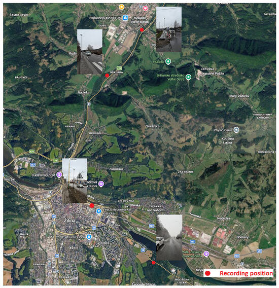
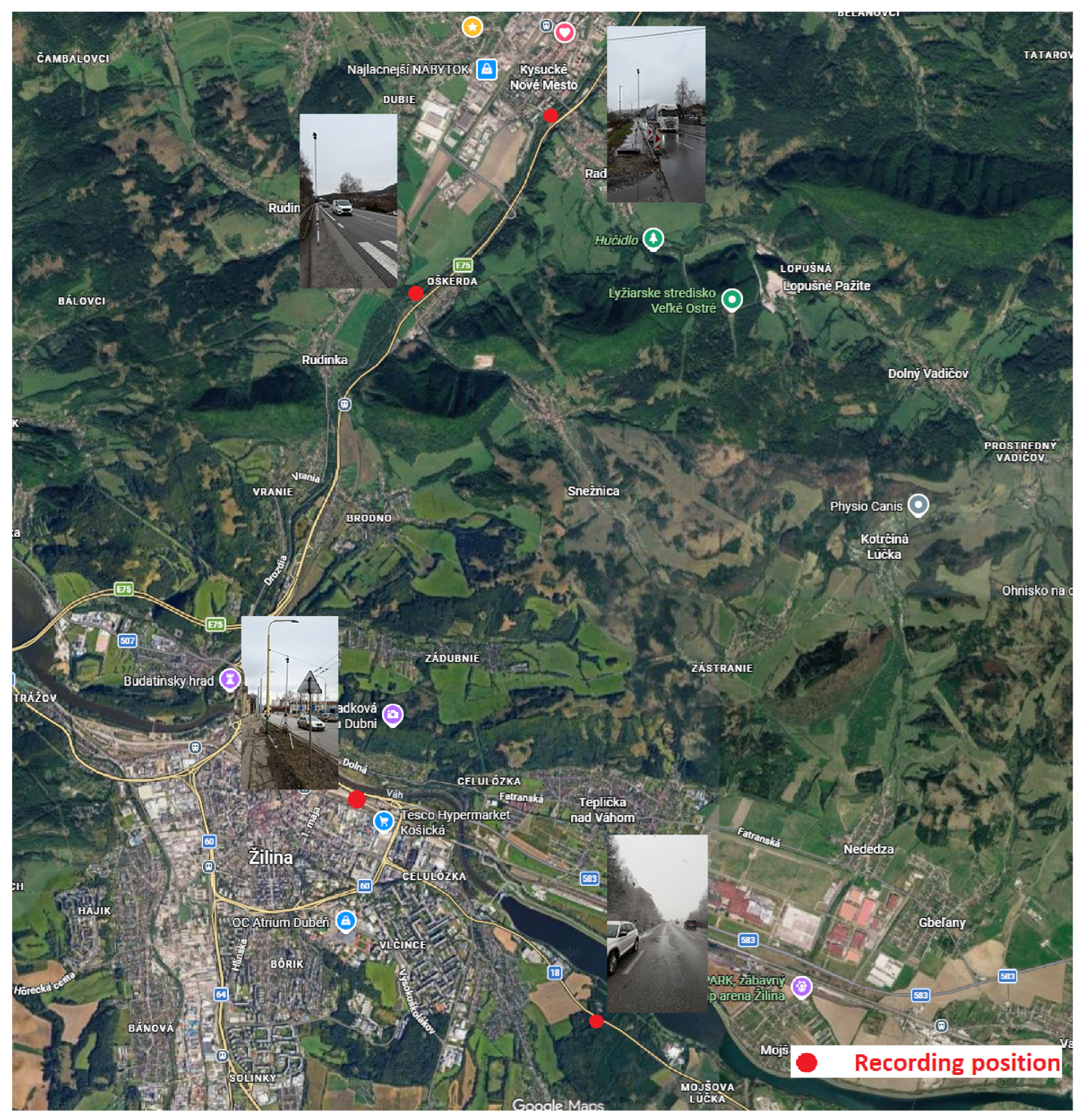
We collected NSVD [39] at four fixed roadside sites in the Žilina Region of northern Slovakia. Three sites were located along the I/18 and I/11 first-class road corridors. The fourth site was situated in the center of Žilina. Together, the sites cover urban, suburban, and rural road environments. Table 2 lists their locations and road classifications. Figure 1 shows their geographic positions together with the corresponding camera views. The I/18 and I/11 locations were selected to capture inter-urban traffic and a higher proportion of goods vehicles. The sites were selected deliberately and do not form a random sample of the regional road network.

Table 2. The four NSVD collection sites.

Site	Road	Coordinates	Environment
Trnové (Žilina)	I/18 (E50)	49.2026, 18.7932	urban edge
Oškerda (Kys. N. Mesto)	I/11 (E75)	49.2766, 18.7633	rural/transit
Radoľa (Kys. N. Mesto)	I/11 (E75)	49.2959, 18.7860	rural/transit
Žilina center (Hviezdoslavova)	urban	49.2265, 18.7470	city (buses)

Figure 1. Locations of the four NSVD collection sites in northern Slovakia. Red points mark the recording positions and the insets show the corresponding camera views. Base map and map data: Google Maps.

Two features of the data collection campaign shaped the composition of the released dataset. First, too few buses passed the roadside sites to support a dedicated class. The city-center site at the bus station was therefore added, with the result that bus annotations are concentrated at that one position. Second, although each recording session was scheduled for a target weather condition, that condition could not be maintained for an entire session. Recordings were therefore repeated across several days, and each weather label was tied to the specific positions and days on which the intended condition persisted. Neither of these compositional features constitutes an experimental design.

Recording took place from December 2025 to April 2026 between 08:00 and 14:00. A single Sony FDR-AX43A camera was moved between the four recording sites, and Figure 2 below showing each of these four recording positions. At every site, the camera recorded video at $3840\times 2160$ pixels and 50 frames per second (FPS). Exposure was set manually with a shutter speed of $1/1750$ s. The camera was mounted approximately $4.5$ m above the road surface, with a vertical angle of $27°$ and a horizontal angle of $20$–$25°$. Lateral distance from the lane axis ranged from about $2.8$ to $3.1$ m. This elevated, oblique viewpoint produces an object-size distribution distinct from that of an on-board camera and keeps long vehicles fully inside the frame while still providing a clear view of approaching traffic.

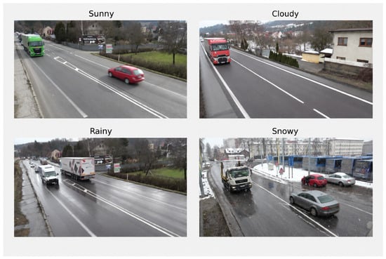
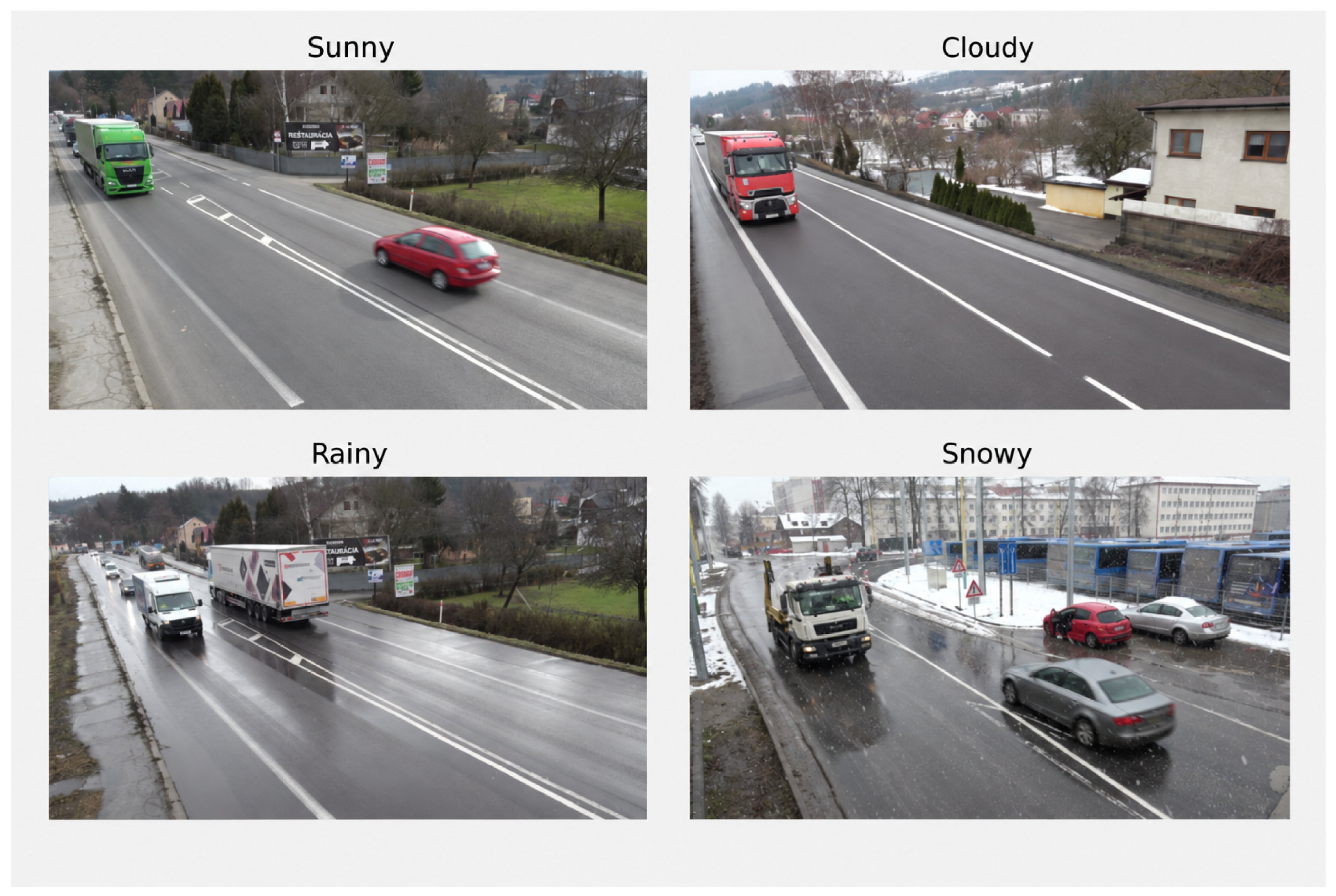
Figure 2. Examples from the four visual weather labels used in NSVD.

The 19 video recordings were partitioned into three-hour clips, yielding approximately $\mathrm{55,000}$ candidate frames. Frames were exported with VLC and inspected visually. The subset of 8000 images was selected with a target of 2000 images per visual weather label. Frames exhibiting severe motion blur, sensor artifacts or complete occlusion were discarded. The selection also considered scene content and vehicle sharpness. No information about class balance or model difficulty was used when individual frames were chosen. However, manual selection can favor clearer examples and recurring traffic situations. No automated sharpness measure or near-duplicate filter was applied at collection time. An audit of the release is reported below.

The 8000 images were cut from several independent recordings made on different days at the four sites under the conditions described above, and not from a single continuous session. Every exported frame carries a candidate-frame index, running from 1 to $\mathrm{59,088}$ across the release. The mapping from the 50 FPS stream to the exported candidates and the wall-clock interval corresponding to one index step were not recorded, so separations between partitions are reported solely in index units and do not represent measured time gaps.

The source videos were recorded in ultra-high definition. The public dataset contains downsampled images at at $1920\times 1088$ pixels with faces and license plates blurred.

The annotation guide defines five visual vehicle classes, four of which are present in the current dataset release. The fifth class, motorcycle, is unpopulated because the campaign was conducted from December to April, outside the season in which powered two-wheelers are common on these roads. At most about six motorcycles appear across all recordings, which is too few for reliable training or evaluation. The class identifier is kept so that a summer extension can add motorcycles without renumbering, and the class is excluded from training and from every reported metric. Table 3 summarizes the visual classification rules, which are based on body style, relative dimensions, and apparent use. They do not identify a legal vehicle type, registered mass, or seating capacity.

Table 3. Visual class rules used in NSVD.

Class	Visual Rule	Status
car	Passenger car body, including sport utility vehicles and pickups	populated
van	Van or minivan body, including small passenger vans	populated
bus	Large passenger vehicle or a bus body on a larger chassis	populated
truck	Cargo body, tractor unit or flatbed	populated
motorcycle	Powered two-wheeler	unpopulated

The separate van class is defined to capture van-bodied vehicles that would otherwise be assigned to car or truck. Minivans and minibuses built on a passenger-van body are included in this class. Light vehicles with a flatbed are labeled truck, while larger passenger vehicles built on a truck-like chassis are labeled bus. These rules provide a consistent visual taxonomy for NSVD.

The van class was retained because van-bodied vehicles occur frequently in the recordings but have no separate output in an MS COCO detector. Merging them with cars or trucks prevents their performance from being evaluated separately. NSVD, therefore, treats van as a distinct visual class and reports how alternative mappings affect the results. The class is not an exact equivalent of the legal N1 category because registered mass and vehicle purpose cannot be verified from an image.

Each image is annotated with one of four visual weather condition labels: sunny, cloudy, rainy, or snowy. The full release contains 2000 images per label category. Annotators assigned the label corresponding to the dominant appearance of the road area. Borderline cases, such as wet asphalt without visible rainfall, were labeled as cloudy. These labels reflect visual appearance and are not derived from meteorological measurements. Representative examples are shown in Figure 2.

The initial bounding boxes were produced by an ensemble of detection models. Two expert annotators then reviewed the draft annotations in the Computer Vision Annotation Tool (CVAT) and resolved disagreements to produce a single final label set. The released dataset contains $\mathrm{70,772}$ human-reviewed bounding boxes. Because independent annotation versions were not retained, inter-annotator agreement could not be computed. In this work, the term human-reviewed denotes that an expert inspected and corrected the model-generated boxes.

To assess the quality of the released annotations, two of the authors independently re-annotated a random subset of 300 images without access to the released boxes or any detector outputs. Of the 2700 released boxes present on these images, 54 had an incorrect class label and 27 were substantially misplaced, resulting in 81 boxes ($3.0$ %) that required correction. The reference annotation contained 2727 vehicles: every released box was matched by a corresponding reference box, and 27 vehicles ($0.99$ % of the reference set) lacked a released box. The mean intersection-over-union (IoU) over the 2700 matched pairs was $0.85$, which is close to the range of $0.87$–$0.88$ reported in previous re-annotation studies [40,41].

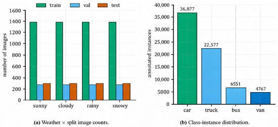
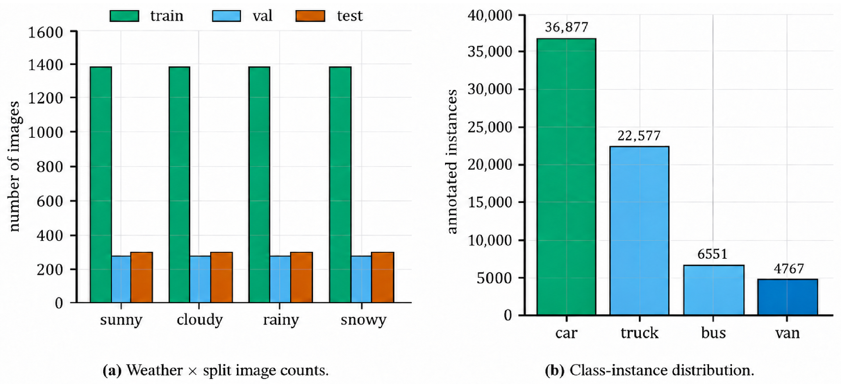
The four visual weather labels contain equal numbers of images, but object-level class distributions remain unbalanced. In total, NSVD comprises $\mathrm{36,877}$ car, $\mathrm{22,577}$ truck, 6551 bus, and 4767 van bounding boxes. Uniform image-level splits therefore do not provide balanced class coverage. Figure 3 illustrates the distribution of images across training splits, alongside object counts for four classes.

Figure 3. Composition of the NSVD dataset. (a) Distribution of benchmark images categorized by visual weather condition and training split. (b) Total object counts across the four populated classes in the full release.

A random image split was avoided because neighboring video frames can be highly similar. Images were therefore grouped by visual weather label and by source folder (the vehicle-class export folder, not a recording session). Within each group, the frames were ordered by candidate-frame index, and contiguous blocks were assigned to the training, validation, and test sets with a target ratio of 70:15:15. A total of 146 frames at the block boundaries were left unassigned to reduce immediate temporal overlap between the adjacent blocks. The final split distribution is presented in Table 4. The release contains 8000 images, of which 7854 are assigned to the benchmark partitions.

Table 4. Predefined same-viewpoint benchmark split by visual weather label. The 146 block-boundary images belong to no partition.

Split	Images	Sunny	Cloudy	Rain	Snow
Train	5527	1384	1380	1384	1379
Val	1128	283	281	284	280
Test	1199	301	299	300	299

A fixed boundary buffer does not guarantee independence, so we report the separation the split achieves and audit the release for repeated content. Across the 19 weather × source-folder groups that span all three partitions, the minimum candidate-frame index distance is 37 at the train–validation boundary and 79 at the validation–test boundary (medians of 362 and 567). Between training and test images, the pair that determines the reported score, the smallest distance is 85. In every group of more than six images it is at least 3753.

No two released images are byte-identical. A global 64-bit perceptual hash over all 8000 images is uninformative on its own, because the fixed camera causes the hash to be dominated by the static background. Candidate pairs within a Hamming distance of 10 were therefore re-ranked by the agreement of their ground-truth boxes (fraction of boxes matched by a same-class box at IoU ≥ 0.5). Seventeen cross-partition pairs reached this threshold. Visual inspection confirmed that each pair shows the same background occupied by different vehicles. No repeated vehicle passage was identified. The screening procedure cannot detect a passage that reappears at a substantially different image position, and therefore only bounds, rather than excludes, this failure mode.

Spacing inside a block is a weaker concern. Consecutive released frames within the same block have a median separation of 27 candidate-frame indices, with quartiles of 11 and 70. Nevertheless, $3.1$% of neighboring pairs are only one index apart, and $10.9$% lie within five indices. Frames belonging to the same block are therefore correlated, as expected for a fixed camera, so the raw image count overstates the effective sample size of a partition. This intra-block correlation does not transfer information across partitions boundaries, which is what the boundary buffer and the duplicate screen address.

The test partition is drawn from the same data collection sites that appear in training set. Consequently, models observe the same road geometry and backgrounds at both training and test time, and the split does not prevent background memorization. The benchmark therefore evaluates same-viewpoint performance. Generalization to before unseen site is evaluated in Section 4.5. The released dataset preserves the final partition assignments, and a per-image manifest carries visual weather label, candidate-frame index and site identifier of every image.

Table 5 presents the weather distribution across four cameras: all $2000$ rain images and 1993 of the 2000 sunny images come from Radoľa, whereas the city-center camera contains no rain data.

Table 5. Number of images per camera by weather label.

Camera	Sunny	Cloudy	Rain	Snow
Radoľa	1993	723	2000	910
Žilina center	7	224	0	717
Oškerda	0	734	0	0
Trnové	0	319	0	373
All	2000	2000	2000	2000

3.2. Van-Aware Evaluation

The populated NSVD classes are car, van, bus, and truck. MS COCO contains the classes car, bus, and truck, but does not include van. A direct comparison, therefore, requires a clear rule for handling van annotations.

Protocol A evaluates the three populated classes shared by both datasets (car, bus, and truck) and produces the common-class score. Van ground-truth boxes are ignored, and van predictions are removed before evaluation. Because COCO evaluation matches detections one category at a time, an ignore region suppresses a false positive only within its own category. It does not suppress a car or truck prediction that overlaps an ignored van. We implement this rule with the COCO iscrowd flag. A van box is written into the car category with iscrowd $=1$. Consequently, a car prediction overlapping a van is counted neither as a true positive nor a false positive, while a truck prediction overlapping it remains a false positive. This is a category-specific treatment of van, not a class-agnostic ignore region. All other unmatched predictions are evaluated normally.

We audited this implementation. An earlier version of the converter set ignore $= 1$ but not iscrowd, which COCOeval does not read, so van boxes were treated as car ground truth. Re-evaluating nine of the eleven checkpoints with the corrected converter changed their common-class and four-class ${\mathrm{mAP}}_{50:95}$ by at most $0.002$ after rounding. The change is small because the detectors typically emit a low-confidence car boxes on most van-bodied vehicles. The benchmark tables therefore retain the earlier evaluation results, while all subsequently added experiments use the corrected converter. Class-wise and object-size averages are more sensitive (shifts of up to 0.05 for large objects), so the comparisons in Section 4.1 employ a single consistent evaluator on both sides.

Protocol B evaluates all four populated NSVD classes and is used for models trained with the NSVD taxonomy. Protocol B produces the four-class score. The empty motorcycle class is excluded from both protocols.

All models are evaluated on the same test split with pycocotools. Before scoring, predictions and ground truth are converted to the protocol-specific label set described above. The identical deterministic conversion is applied to every model evaluated under a given protocol, thereby separating changes in class definition from changes in the detector itself.

3.3. Evaluation Metrics

Detection quality is measured with the standard COCO evaluation in pycocotools. The primary metric is mean average precision (mAP) over intersection-over-union thresholds from 0.50 to 0.95 in steps of 0.05. Intersection over union (IoU) measures the overlap between a predicted box $\widehat{B}$ and a ground-truth box B as

$$\mathrm{IoU}(B,\widehat{B})={\displaystyle \frac{|B\cap \widehat{B}|}{|B\cup \widehat{B}|}}.$$

(1)

For class c and IoU threshold $\tau$, precision and recall are computed from the true-positive, false-positive, and false-negative counts. They are defined as

$$\mathrm{Precision}={\displaystyle \frac{\mathrm{TP}}{\mathrm{TP}+\mathrm{FP}}},\mathrm{Recall}={\displaystyle \frac{\mathrm{TP}}{\mathrm{TP}+\mathrm{FN}}}.$$

(2)

Let $P_c(r,\tau )$ denote precision for class c at recall level r. COCO uses the interpolated precision envelope at 101 recall levels and calculates average precision as

$${\mathrm{AP}}_c\left(\tau \right)={\displaystyle \frac{1}{101}}\sum _{r\in \{0,0.01,\dots ,1\}}\underset{\tilde{r}\ge r}{\max }{P}_c(\tilde{r},\tau ).$$

(3)

The primary metric averages this value across C evaluated classes and ten IoU thresholds

$${\mathrm{mAP}}_{50:95}={\displaystyle \frac{1}{10C}}\sum _{\tau \in \{0.50,0.55,\dots ,0.95\}}{\displaystyle \sum _{c=1}^C}{\mathrm{AP}}_c\left(\tau \right).$$

(4)

We also report ${\mathrm{mAP}}_{50}$, class-wise AP, and AP for the COCO small, medium, and large object bands. Class-wise AP is the mean of ${\mathrm{AP}}_c\left(\tau \right)$ over the same ten IoU thresholds.

One source of variation is reported. Training variability is given as the mean and sample standard deviation over three random seeds. This quantity is used to assess whether an observed difference exceeds normal run-to-run noise. Estimates based on classes with limited support are marked as such. Training variability is not used to claim statistical significance or equivalence, because three runs are insufficient to support such claims.

Computational results include the number of parameters, floating-point operations (FLOPs) at an input size of $960\times 960$ pixels and frames per second (FPS).

3.4. Implementation Details

All detectors use the same NSVD split, image size, and epoch count, and the same random seed except where a configuration is repeated over seeds. They do not use equal computation or an identical optimizer. The YOLO models use stochastic gradient descent (SGD) with an initial learning rate of 0.01 and a cosine schedule. Mosaic augmentation is disabled for the last ten epochs. RT-DETR uses its default AdamW optimizer with an initial learning rate of ${10}^{-4}$ and a cosine schedule. Models were trained for 40 epochs at $960\times 960$ pixels on NVIDIA RTX 3090 and RTX 4090 graphics processing units, at an effective batch of 64, reached by gradient accumulation where the memory required a smaller micro-batch. All timing in Section 4.7 was measured on one RTX 4090. Table 6 summarizes the settings that were recorded.

Table 6. Recorded training configuration. Models share the split, input size, epoch count and effective batch, and each family keeps its own optimizer.

Model	Initialization	Input	Epochs	Optimizer	Effective Batch
YOLOv8, v9, v10, 11, 12, 26	COCO	960	40	SGD, rate 0.01, cosine	64
YOLO11-M control	random	960	40	SGD, rate 0.01, cosine	64
RT-DETR-L	COCO	960	40	AdamW, rate ${10}^{-4}$, cosine	64
RT-DETR-X	COCO	960	40	AdamW, rate ${10}^{-4}$, cosine	64

A minimal accuracy difference between single runs cannot establish an ordering of models. Therefore, four configurations—YOLO11-S, YOLO11-M, RT-DETR-L, and RT-DETR-X—were each trained with three seeds (0, 1, and 2) to ensure repeated runs for both model families. All other experimental settings were held fixed across the three runs, including the data split, initialization, input size, number of epochs, batch size, data augmentation, checkpoint selection rule, and software library versions. Section 4.2 reports the mean and standard deviation of these four configurations, evaluated with the corrected converter. The detailed analyses use the seed-0 run of YOLO11-M. The remaining seven configurations are single runs. The provenance, software versions, and checkpoints of all benchmarked model families are summarized in Table 7.

Table 7. Provenance of the benchmarked checkpoints. The listed versions identify the Ultralytics releases from which the checkpoints were obtained.

Model Families	Source and Version	Checkpoints
YOLOv8, YOLOv10, YOLO11, RT-DETR	Ultralytics 8.3.0	yolov8{s,m}, yolov10{s,m}, yolo11{s,m}, rtdetr-{l,x}
YOLOv9-C, YOLO12, YOLO26	Ultralytics 8.4.104	yolov9c, yolo12m, yolo26m

Because each family keeps the optimizer its authors ship, comparisons between families confound architecture with the training recipe. One controlled pair bounds this contribution. YOLO11-M was retrained with AdamW under the same split, initialization, budget and augmentation, using the learning rate and weight decay taken from documented defaults and fixed before training. Under that recipe, YOLO11-M reaches $0.874$ on Protocol A, compared with $0.886$ for SGD (both under the corrected converter of Section 3.2). The difference of $0.012$ is about one-fifth of the $0.062$ gap between YOLO11-M and RT-DETR-L and about five times the seed standard deviation of the SGD runs. It is therefore unlikely to be seed noise, although the AdamW run is a single seed. The experiment measures training recipe sensitivity for YOLO11-M, not a general optimizer effect.

YOLO11-M was selected for the detailed analyses so that transfer, taxonomy, and weather results use one reference detector. RT-DETR-L and RT-DETR-X were included as available real-time transformer configurations with higher computational cost. Validation ${\mathrm{mAP}}_{50:95}$ changed by less than 0.005 during the last ten epochs of the main YOLO11-M run, and a 100-epoch control changed four-class ${\mathrm{mAP}}_{50:95}$ by 0.005, so a longer schedule would not have changed its point estimate materially.

A second YOLO11-M control used random initialization. It retained the same NSVD split, image size, epoch count, optimizer, and seed setting as the COCO-initialized fine-tuning run. This control separates the value of training on NSVD from the additional value of COCO initialization under the recorded budget.

4. Results

We first evaluate how well COCO-pretrained detectors transfer to NSVD and how much performance is recovered by training on the target data. We then compare the detector configurations, examine the treatment of the van class, and report results for the four visual weather labels. Four further subsections address the site-disjoint evaluation, the DAWN experiment, model timing and an error analysis. Unless stated otherwise, all results are obtained on the NSVD test split using the pycocotools evaluator.

As shown later, YOLO11-M is a recent medium-sized YOLO checkpoint that offers a favorable balance of peak performance and computational cost. Focusing the remaining analyses on this architecture maintains consistency across experiments and avoids mixing results from different model families.

4.1. In-Domain Fine-Tuning

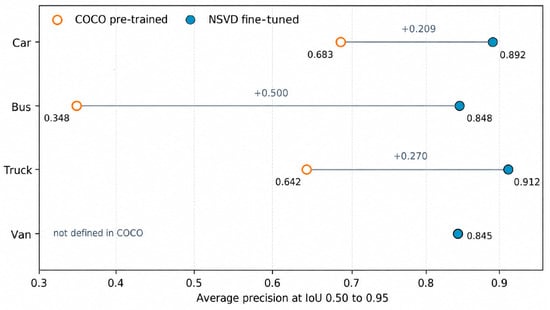
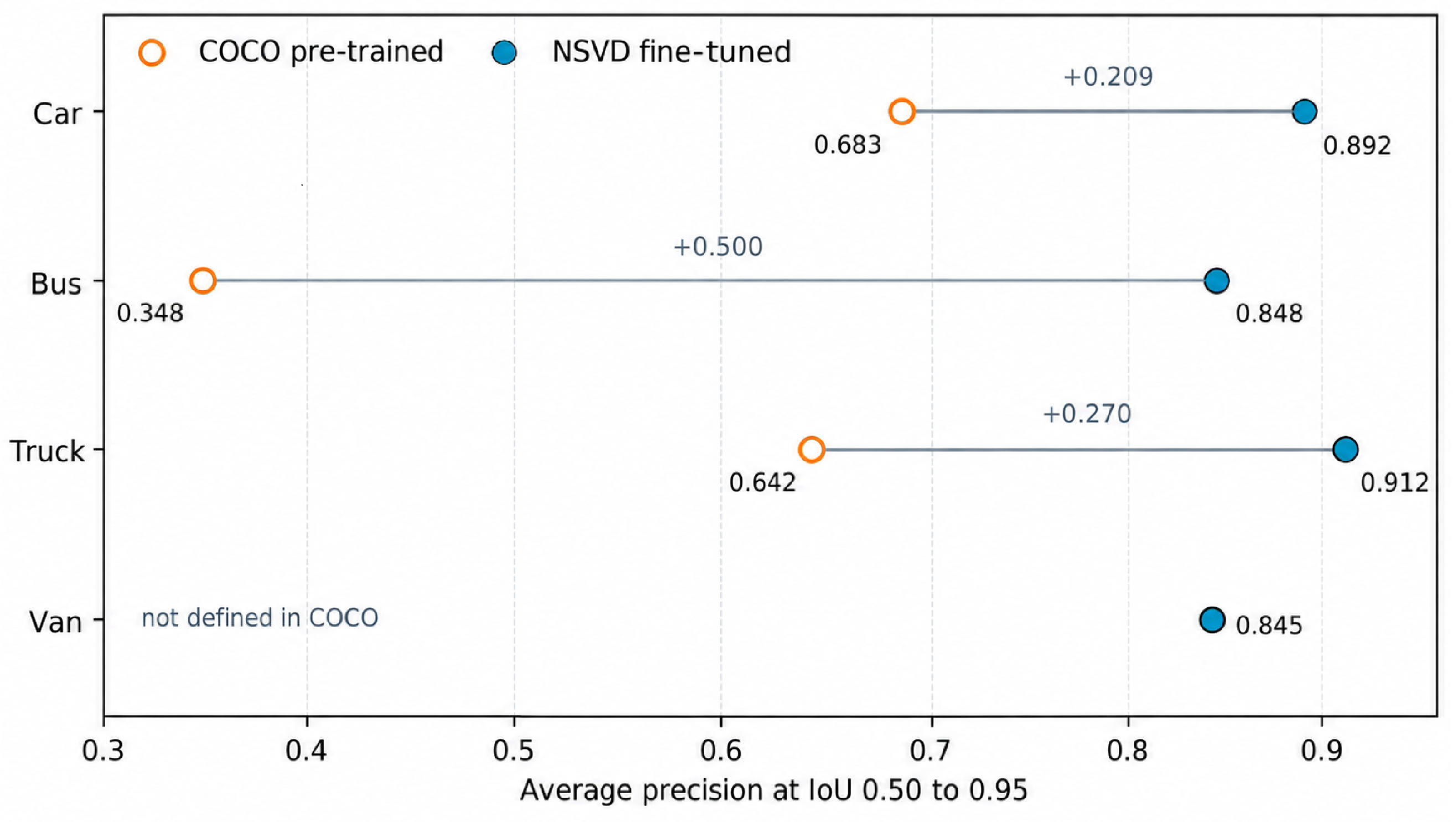
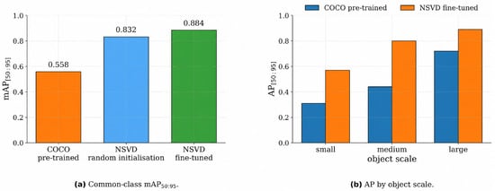
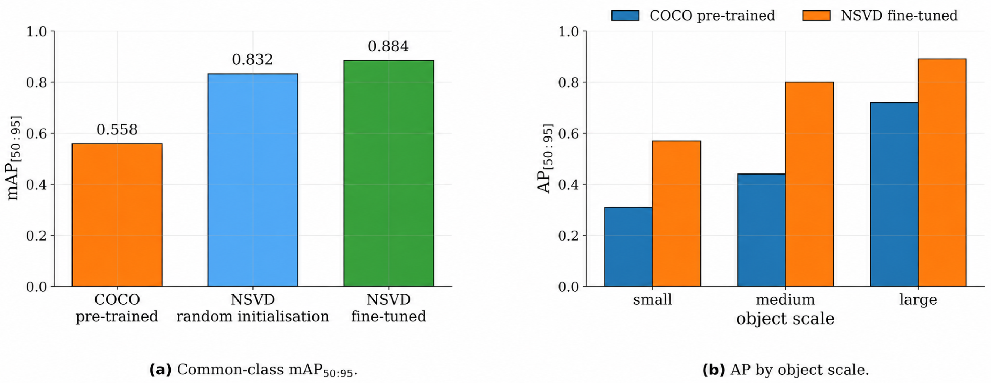
Without fine-tuning, the COCO-pretrained YOLO11-M achieved a common-class ${\mathrm{mAP}}_{50:95}$ of 0.558 on NSVD test set. After fine-tuning on NSVD, the same model achieved 0.884 (Table 8). AP increased for all three shared vehicle classes. The AP value for car increased from 0.683 to 0.892, bus AP from 0.348 to 0.848, and truck AP from 0.642 to 0.912. Van has no COCO-pretrained result because COCO does not contain this class. Figure 4 shows the class-wise results. Differences in the magnitude of the gains should not be interpreted solely as differences in class difficulty, because the number, scale, and visual diversity of objects also vary across classes.

Table 8. Transfer from COCO to the NSVD evaluation under Protocol A.

Model	Regime	${\mathbf{mAP}}_{50:95}$	Car AP	Bus AP	Truck AP
YOLOv8-M	COCO pretrained	0.545	0.665	0.349	0.621
YOLOv10-M	COCO pretrained	0.533	0.674	0.295	0.630
YOLO11-S	COCO pretrained	0.493	0.626	0.272	0.580
YOLO11-M	COCO pretrained	0.558	0.683	0.348	0.642
YOLO26-M	COCO pretrained	0.560	0.695	0.358	0.626
YOLO11-M	NSVD fine-tune	0.884	0.892	0.848	0.912
$\Delta$ vs. COCO pretrained		+0.326	+0.209	+0.500	+0.270

Figure 4. Class-wise AP before and after NSVD fine-tuning.

Fine-tuning of YOLO11-M also improved performance across all object-size bands. AP increased from 0.31 to 0.57 for small objects, from 0.44 to 0.80 for medium objects, and from 0.72 to 0.89 for large objects. Although small objects showed a clear improvement, they remained the most difficult group to detect (Figure 5). These groups are based on bounding-box area in the image and do not directly represent distance from the camera.

Figure 5. Transfer evaluation for YOLO11-M under Protocol A: (a) common-class performance across training regimes. (b) AP scores by object size.

The random-initialization control achieved a common-class ${\mathrm{mAP}}_{50:95}$ of 0.832 after training from scratch on NSVD. This value was 0.274 higher than the COCO-pretrained result and 0.052 lower than fine-tuning from COCO weights. Under the tested training settings, the majority of the improvement came from training on NSVD. COCO initialization contributed a smaller additional gain.

The remaining COCO-pretrained checkpoints produced common-class ${\mathrm{mAP}}_{50:95}$ scores between 0.493 and 0.560. After fine-tuning on NSVD, all models showed a clear performance gain, with common-class ${\mathrm{mAP}}_{50:95}$ rising to the range 0.863–0.882.

4.2. Cross-Architecture Benchmark

Table 9 compares the eleven detector configurations evaluated in this study. The benchmark includes models from the YOLOv8, YOLOv9, YOLOv10, YOLO11, YOLO12, and YOLO26 families [5,16,42,43,44], as well as the transformer-based RT-DETR-L and RT-DETR-X models [7]. Checkpoint provenance for all models is listed in Table 7.

Table 9. Detector benchmark on the NSVD test set with parameter counts and floating-point operations at 960 pixels.

Model	Params (M)	FLOPs (G)	Common-Class ${\mathbf{mAP}}_{50:95}$	Four-Class ${\mathbf{mAP}}_{50:95}$
YOLOv8-S	9.80	53.0	0.819	0.817
YOLOv8-M	23.20	153.0	0.863	0.854
YOLOv9-C	25.50	233.0	0.842	0.836
YOLOv10-S	8.10	56.0	0.864	0.861
YOLOv10-M	16.50	144.0	0.876	0.874
YOLO11-S	9.43	48.5	0.867	0.857
YOLO11-M	20.06	153.5	0.884	0.874
YOLO12-M	20.10	152.0	0.867	0.858
YOLO26-M	21.80	168.0	0.882	0.876
RT-DETR-L	32.82	238.7	0.822	0.819
RT-DETR-X	67.31	518.5	0.831	0.828

Common-class ${\mathrm{mAP}}_{50:95}$ scores range from 0.819 to 0.884, with YOLO11-M achieving the highest common-class accuracy. On the four-class metric, YOLO26-M obtains the highest score (0.876), followed by YOLOv10-M and YOLO11-M (both 0.874).

Table 10 reports the mean and standard deviation for the four configurations that were trained repeatedly with three different seeds. These means agree with the corresponding single-run values in Table 9 within $0.002$. On the common-class metric, the seed standard deviation is $0.001$–$0.002$ for the YOLO11 models but rises to $0.009$ for RT-DETR-X and $0.016$ for RT-DETR-L (the latter driven mainly by a single outlier run). Differences of approximately $0.002$ among the leading YOLO configurations are therefore of the same magnitude as the observed seed variability and do not support a reliable ranking. The remaining seven configurations are single-run results from which no ordering is inferred. Smaller models are likewise not ranked against larger ones. Note that YOLO11-S and YOLO11-M are indistinguishable in inference time at batch size 1 on RTX 4090 (Section 4.7), so FLOPs do not translate directly into time.

Table 10. Mean and sample standard deviation of ${\mathrm{mAP}}_{50:95}$ over three random seeds for the four repeated configurations.

Model	Seeds	Common-Class ${\mathbf{mAP}}_{50:95}$	Four-Class ${\mathbf{mAP}}_{50:95}$
YOLO11-S	3	$0.868\pm 0.001$	$0.857\pm 0.003$
YOLO11-M	3	$0.885\pm 0.002$	$0.875\pm 0.001$
RT-DETR-L	3	$0.823\pm 0.016$	$0.819\pm 0.015$
RT-DETR-X	3	$0.832\pm 0.009$	$0.828\pm 0.007$

Under the present protocol, the two RT-DETR models score 0.036–0.062 below the repeated YOLO11 configurations, which is more than twice the largest observed seed standard deviation. They also use a different optimizer and are at the high end of the evaluated computational range, so the gap mixes architecture with training recipes. The controlled pair of Section 3.4 bounds the recipe contribution for one model at $0.012$ and does not make Table 9 an equal-budget architecture comparison. Under the tested settings, the leading YOLO configurations combine higher ${\mathrm{mAP}}_{50:95}$ with lower computational cost than the two RT-DETR configurations. This is presented as a descriptive comparison of the practical configurations trained in this study, not as a general ranking between detector families.

4.3. Effect of Van Class Mapping

Table 11 compares four treatments of the van class using identical YOLO11-M predictions. Ignoring vans averages performance over three classes and excludes all van-related errors from the score. Mapping vans to either car or truck class likewise averages three classes, but first merges the van bounding boxes with the target class. Treating vans as a separate class averages four classes and retains its errors as a distinct part of the evaluation.

Table 11. Effect of van handling on the evaluation of the same YOLO11-M predictions. A dash means that the van is not scored separately, and bus AP is unaffected.

Van Handling	Evaluation Labels	Car AP	Truck AP	Van AP	Reported ${\mathbf{mAP}}_{50:95}$
ignore van	car, bus, truck	0.892	0.912	–	0.884
map van to car	car+van, bus, truck	0.899	0.912	–	0.886
map van to truck	car, bus, truck+van	0.892	0.910	–	0.883
separate van	car, van, bus, truck	0.892	0.912	0.845	0.874

Under the individual-class protocol, van achieves the lowest AP of 0.845 as well as the lowest four-class ${\mathrm{mAP}}_{50:95}$ of 0.874. Ignoring van raises the ${\mathrm{mAP}}_{50:95}$ to 0.884 because the lower van score is no longer included in the mean. Mapping vans to cars increases car AP from $0.892$ to $0.899$ and yields an ${\mathrm{mAP}}_{50:95}$ of $0.886$. Mapping vans to trucks decreases truck AP from $0.912$ to $0.910$ and yields an ${\mathrm{mAP}}_{50:95}$ of $0.883$. The small changes in the reported mean show why mAP alone cannot reveal how van-shaped vehicles were treated during evaluation. Protocol B is therefore used when the aim is to evaluate the full NSVD taxonomy.

4.4. Weather-Resolved Performance

The visual weather labels support two descriptive comparisons. Before fine-tuning, the COCO-pretrained YOLO11-M achieved common-class ${\mathrm{mAP}}_{50:95}$ of $0.672$ (sunny), $0.632$ (cloudy), $0.592$ (rainy), and $0.538$ (snowy). After fine-tuning on NSVD, the same model reached $0.858$ on sunny images and remained above 0.80 on all four subsets (Table 12). A transfer gap is therefore already present under sunny conditions and widens under rain and snow. This comparison, however, does not isolate weather from differences in site, recording conditions, or traffic composition.

Table 12. Common-class ${\mathrm{mAP}}_{50:95}$ by visual weather label for models trained on all labels.

Model	Sunny	Cloudy	Rain	Snow
YOLO11-S	0.827	0.856	0.793	0.853
YOLO11-M	0.858	0.877	0.807	0.871
RT-DETR-L	0.800	0.809	0.782	0.811
RT-DETR-X	0.804	0.822	0.796	0.821

Table 12 reports Protocol A scores after fine-tuning four selected configurations. YOLO11-M ranges from $0.807$ (rainy) to $0.877$ (cloudy). YOLO11-S shows a similar pattern. The narrower spread observed for RT-DETR-L and RT-DETR-X across the labels does not demonstrate greater weather robustness, because the models have different overall detection performance and the subsets differ in viewpoint and class composition.

These values do not measure the effect of weather alone. Table 13 gives the annotation counts and camera composition of each subset. Bus annotations range from 9 boxes in sunny to 1386 in snowy, while truck annotations fall to 209 in snowy against 991–1252 in the other conditions. Each weather label also draws on a different set of cameras, with all rain images coming from the Radoľa camera that contains almost no buses. Weather, viewpoint, and class composition, therefore, vary jointly, and reweighting the subsets cannot disentangle them. We therefore present the condition-specific scores as descriptive results accompanied by their support counts and do not interpret them as pure weather effects.

Table 13. Support behind the weather-resolved results: annotations per class in each test subset and the cameras contributing to each label over the full release.

Test Split	Sunny	Cloudy	Rain	Snow
Images	301	299	300	299
car	1172	1350	1463	1949
bus	9	70	14	1386
truck	1252	991	1080	209
van	202	186	200	112
Cameras (full release)	Radoľa, Žilina center	all four	Radoľa	Radoľa, Žilina center, Trnové

One controlled comparison is available. The Radoľa camera provides test images under all four labels and contains a sufficient number of cars in each. Restricting evaluation to this camera and to the car class alone holds both factors fixed (although recording day and traffic still vary). Under Protocol A, car AP is $0.906$ for sunny, $0.906$ for cloudy, $0.885$ for rainy (a spread of only $0.021$ over 1172–1463 car boxes), and $0.776$ for snowy on 154 boxes from 56 images. With camera and class held constant, the three well-supported labels lie within $0.021$ of each other, suggesting that the wider variation in Table 12 is driven primarily by composition rather than by weather. The snowy result, based on only 56 images, is less informative.

The class-specific results show the same limitation. Bus AP is 0.624 in rain and 0.854 in snow. In contrast, car AP was 0.885 in rain and 0.882 in snow, while truck AP was 0.911 and 0.877. The bus result for rain is based on only 14 boxes and is reported for completeness. It does not support a comparison between rain and snow.

A leave-one-weather-out comparison, in which the model is trained without one weather label and tested on it, is not reported. Withholding the snowy images removes the snowy frames of the Žilina center camera, which supplies almost all buses, and with them 2670 of the 3370 bus boxes in the training partition ($79.2$% of all bus supervision). The corresponding figures for sunny, rainy, and cloudy are only $2.9$%, $1.8$% and $16.1$%. Any comparison labeled snowy would therefore contrast a model trained with substantial bus supervision against one trained with almost none, and would not measure generalization to snow.

4.5. Site-Disjoint Evaluation

To measure performance at a site the model has not seen, we add a leave-one-site-out evaluation of YOLO11-M over the four cameras (one per site) listed in Table 5. Each fold holds out one camera entirely. All of its images form the test set. Training and validation sets are drawn exclusively from the remaining cameras after removing every image within 30 candidate-frame indices of a held-out frame in the same weather and source-folder group, and are split 85:15 at random. Every fold is initialized from the COCO checkpoint, and no threshold or checkpoint is selected on the held-out camera.

A fold cannot be compared directly with the model trained on the predefined split, because that model has already seen most of the fold’s test images. We therefore evaluate both models only on the images that belong to the held-out camera (disjoint-viewpoint) and to the original predefined test partition (same-viewpoint)—images that neither model has trained on. This comparison is possible for Radoľa (940 images) and for the city center with (257 images). The lower block of Table 14 presents this paired result. Holding out Radoľa in the disjoint-viewpoint setup lowers common-class ${\mathrm{mAP}}_{50:95}$ from $0.825$ to $0.624$, and holding out the city center lowers it from $0.837$ to $0.372$. The same-viewpoint reference is below the $0.884$ obtained on the full test partition because each subset has its own class balance (26 bus boxes for Radoľa, 18 truck boxes for the city center). The upper block of the table reports the remaining two folds, each evaluated on every image of its held-out camera.

Table 14. Leave-one-site-out folds. Train and Test are image counts. ${\mathrm{mAP}}_{50:95}$ covers car, bus, and truck under Protocol A, and van is scored under Protocol B without entering the mean.

Held Out	Train	Test	${\mathbf{mAP}}_{50:95}$	Car	Bus	Truck	Van
Each fold on every image of its held-out camera
Radoľa	978	5626	0.594	0.733	0.373	0.676	0.542
Žilina center	5049	948	0.298	0.567	0.045	0.282	0.549
Oškerda	5452	734	0.876	0.882	0.916	0.829	0.800
Trnové	5274	692	0.698	0.806	0.561	0.726	0.646
Paired, on the images shared with the predefined test partition
Radoľa same-viewpoint	5527	940	0.825	0.894	0.669	0.912	0.851
Radoľa disjoint	978	940	0.624	0.761	0.412	0.699	0.571
Žilina center same-viewpoint	5527	257	0.837	0.898	0.855	0.757	0.822
Žilina center disjoint	5049	257	0.372	0.517	0.034	0.565	0.588

Holding a camera out removes its training images as well as its site, so the performance drop cannot be attributed solely to a site effect, and the folds also differ substantially in the amount of training data that is removed with the camera. We therefore interpret the results primarily through car AP, the only class that every camera supplies well. Oškerda retains car AP at $0.882$ (versus approximately $0.89$ on the predefined benchmark), showing that a completely unseen site is not necessarily out of reach. Trnové, whose fold keeps 5274 training images, falls to $0.806$, about $0.09$ below the benchmark, again at the site the model has never seen. Radoľa contributes the majority of the release. Its fold retains only 978 training images and falls to $0.733$, a drop that is confounded with the severe reduction in training data.

The city center is the informative case. Its fold retains 5049 training images (approximately nine tenths of the original partition) yet scores only $0.298$. The city-center camera supplies almost all bus annotations (Table 5), so bus AP collapses to $0.045$ on the 6351 bus boxes of that test set, which is a class left without any training examples. But car AP, which every camera supplies well, also falls from about $0.89$ to $0.567$, and on the paired images from $0.898$ to $0.517$. Neither a smaller training set nor missing supervision explains that. The city-center scene differs enough from the roadside scenes that the detector trained without it fails to generalize.

4.6. Supporting Evaluation on DAWN

We repeated the same pre-trained and target-domain fine-tuning comparison on DAWN [28] to check whether the benefit of labeled target data also appears on a second road-image dataset. The experiment uses the car and truck classes from the fog, rain, and snow subsets. From an initial pool of 704 images, four images that contained neither a car nor a truck annotation were removed. The remaining 700 images were partitioned at the image level into 489 training, 105 validation, and 106 test images. We evaluated the COCO-pretrained YOLO11-M without adaptation and fine-tuned another model on the DAWN training set.

Fine-tuning increased common-class ${\mathrm{mAP}}_{50:95}$ from 0.453 to 0.538 and improved both classes (Table 15). The absolute gain of 0.085 is smaller than the gain of 0.326 observed on NSVD. These values cannot be used to compare the distance between the two domains because the datasets and split procedures differ. The random image split and the removal of negative images further limit the interpretation.

Table 15. DAWN experiment. All three regimes are scored on the same 106 held-out images at 960 pixels. The two fine-tuned rows differ only in their initialization.

Regime	DAWN ${\mathbf{mAP}}_{50:95}$	AP50	Car AP	Truck AP
COCO pretrained	0.453	0.665	0.521	0.386
Fine-tuned on DAWN, COCO initialization	0.538	0.804	0.623	0.454
Fine-tuned on DAWN, NSVD initialization	0.536	0.827	0.614	0.458

When the same fine-tuning recipe is applied to a model initialized from the NSVD checkpoint, the resulting ${\mathrm{mAP}}_{50:95}$ is $0.536$, essentially identical to the $0.538$ obtained from COCO initialization. Thus, NSVD weights initialize a DAWN model as effectively as COCO weights. In contrast, the NSVD-trained detector applied to DAWN images without any adaptation fails to transfer. The experiment therefore supports target-domain training and the use of the release as an initialization, and it does not validate NSVD as a general detector.

4.7. Efficiency

Table 16 reports timing on one RTX 4090 with a batch size of 1 and an input size of 960 pixels. The four timed models span the computational range of the benchmark: a compact configuration, the reference detector, and the two transformer configurations. Measurements were obtained with host-side timers around device synchronization after 50 warm-up iterations. YOLO11-S and YOLO11-M are indistinguishable at $12.6$ and $13.0$ ms, a difference smaller than the run-to-run variation of the faster model (SD = $1.20$), and both are more than twice as fast as the RT-DETR configurations. Of the four timed models, YOLO11-M has the highest four-class ${\mathrm{mAP}}_{50:95}$ (Table 9).

Table 16. Inference latency and peak memory at batch size 1 and 960 pixels on RTX 4090. Total reports the mean over five blocks of 200 images together with its standard deviation, Network denotes the forward pass alone, Rest includes the preprocessing, transfers and postprocessing, and Peak is the memory allocated by Torch.

Model	Params (M)	FLOPs (G)	Total (ms)	SD (ms)	Network (ms)	Rest (ms)	FPS	Peak (MiB)
YOLO11-S	9.43	48.5	12.61	1.20	6.64	5.98	79.3	140
YOLO11-M	20.06	153.5	13.00	0.02	8.42	4.58	76.9	313
RT-DETR-L	32.82	238.7	31.86	0.05	24.29	7.57	31.4	424
RT-DETR-X	67.31	518.5	36.95	0.22	29.38	7.57	27.1	496

Timing begins with a decoded image in host memory and ends with detections returned to host memory. The measurement includes preprocessing and letterboxing, the transfers in both directions, the forward pass, and each model’s native postprocessing. Disk access, video decoding, network transport and serialization lie outside the measured interval. The reported value is image-to-detection latency on the stated hardware, not roadside-system latency. FPS is simply the reciprocal of this latency for sequential batch-1 processing. No embedded module was evaluated.

The non-network portion of the total latency lies between $4.6$ ms and $7.6$ ms for all four models. For RT-DETR-X it disappears into a 29 ms forward pass, but for YOLO11-S it constitutes 47% of the total. Throughput figures that report only the network therefore overstate the performance attainable by the compact configurations.

4.8. Error Analysis

We analyzed the stored YOLO11-M predictions over the whole test split at a confidence threshold of $0.55$, selected on the validation split, with one-to-one matching at an intersection over union of $0.5$. This answers a different question from the confidence-ranked average precision. Each case is assigned to one category: correct, class error, localization error (overlap between $0.1$ and $0.5$), duplicate detection, background false positive or missed object. Of the $\mathrm{12,307}$ diagnosed cases, $87.3$% are correct, $5.4$% are missed objects, $2.9$% are background false positives, $2.5$% are localization errors, and $1.2$% are class errors and $0.7$% are duplicates (Table 17).

Table 17. Error analysis of YOLO11-M on the test split at an operating threshold of $0.55$. Every detection is placed in one category, and every unmatched ground-truth object is counted as missed.

	Correct	Class Err.	Loc. Err.	Duplicate	Backgr. FP	Missed
All	10741	144	312	89	361	660
share	87.3%	1.2%	2.5%	0.7%	2.9%	5.4%
car	5496	35	37	13	250	396
bus	1328	8	233	62	4	51
truck	3332	31	37	4	100	166
van	585	70	5	10	7	47
small	2216	29	32	6	261	470
medium	4109	55	69	22	89	145
large	4416	60	211	61	11	45

Three concentrations stand out. Van accounts for 49% of all class errors while making up 6% of the cases. Its class-error rate of $9.7$% is more than ten times that of car, truck, and bus, which stay below 1%. A merged taxonomy would not expose this failure mode, which supports keeping the van separate. Small objects carry 71% of the missed objects and 72% of the background false positives, and their miss rate, missed objects over all diagnosed cases of the group, is $15.6$% against $0.9$% for large objects. Localization error is a large-object problem: 68% of it falls there, and bus has a localization-error rate of $13.8$%, consistent with buses being long enough to leave the frame at this viewpoint.

Every image in the current benchmark split contains at least one vehicle. Consequently, the reported metrics do not measure how often a detector produces false positives on completely empty roads. The observed 2.9% background false-positive rate refers exclusively to incorrect detections such as detections on background structures, partial objects, or weather-induced artifacts. The original video recordings have been retained, so a set of verified vehicle-free frames can be extracted in future work.

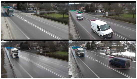
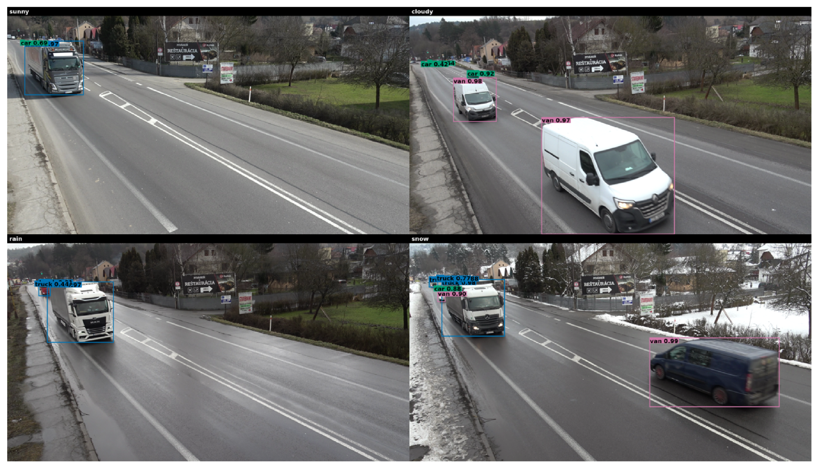
Figure 6 shows example predictions from YOLO11-M. The panels include correct detections and visible errors. They are provided for illustration only and are not intended for comparison across visual weather labels. A systematic analysis of the errors is presented in Table 17.

Figure 6. Illustrative YOLO11-M predictions from one site under the four visual weather labels, including both correct detections and errors.

5. Discussion

The largest performance difference was observed between direct use of the general COCO checkpoint and training on NSVD. For YOLO11-M, common-class ${\mathrm{mAP}}_{50:95}$ increased from 0.558 to 0.884, and most of the gain came from training on NSVD rather than from COCO initialization (Section 4.1). The four-class scores of the eleven fine-tuned configurations ranged from 0.817 to 0.876.

The findings apply to viewpoints represented in the training data. It does not indicate how the NSVD-trained model would perform at a previously unseen camera or in another geographic region. Section 4.5 quantifies the first of these effects: car AP at a withheld camera ranged from $0.882$ at Oškerda to $0.567$ at the city-center site, compared with approximately $0.89$ on the predefined benchmark. A detector should therefore be validated at the specific camera where it will be deployed.

The van analysis shows why class mapping must be reported together with ${\mathrm{mAP}}_{50:95}$. The reported means span only 0.012, but they average different label sets and cannot be interpreted as the same metric. The error analysis further shows that the van class accounts for half of all class errors. Reporting both the common-class result and the full NSVD result makes this difference explicit.

The weather results likewise require careful interpretation. Equal image counts did not produce equal numbers of objects for each vehicle class. Viewpoint, recording, and traffic composition also varied across the visual weather labels, as Table 13 shows. The reported scores therefore characterize the collected subsets rather than isolate the independent effect of weather. Future extensions should balance class coverage within each condition where possible, which in this design means recording each condition from more than one viewpoint. A condition-specific class score should always be reported with the number of annotated objects that support it.

Under the recorded settings, the YOLO configurations provided the better combination of ${\mathrm{mAP}}_{50:95}$ and GPU inference time. This outcome does not establish a general advantage of YOLO over transformer-based detectors. The two families were trained with different optimizers and computational budgets, and the control experiment in Section 3.4 bounds that difference for a single model without removing it. Model-specific tuning could change their observed ranking.

NSVD contains daylight data from one Slovak region recorded between December and April, and its visual weather labels describe appearance, rather than instrumented measurements. The predefined benchmark is a same-viewpoint evaluation whose test partition comes almost entirely from two of the four cameras. Tracking accuracy, counting error and alarm rates per unit time were outside the scope of this study. An NSVD-trained detector applied to the DAWN images without adaptation failed to transfer, whereas the same weights initialize the DAWN model as effectively as COCO weights. The release is therefore intended as the benchmark and initialization for fixed roadside cameras, not as a general-purpose detector. The reported timing figures describe image-to-detections processing on a desktop GPU and do not represent roadside-system latency, and the temporal spacing between partitions is known only in candidate-frame index units.

6. Conclusions

We created and publicly released the Northern Slovakia Vehicle Dataset for the evaluation of vehicle detectors at fixed roadside cameras. NSVD contains 8000 images and 70,772 human-reviewed bounding boxes from four sites in northern Slovakia. It provides four visual weather labels and a separate class for van-bodied vehicles. The predefined benchmark assigns 7854 of the released images to the training, validation, and test partitions. The article also introduces a clear protocol for comparing the NSVD and COCO vehicle classes.

Training YOLO11-M on NSVD increased common-class ${\mathrm{mAP}}_{50:95}$ from 0.558 to 0.884. The tested fine-tuned models produced four-class scores between 0.817 and 0.876. The treatment of van changes what the score measures, so both the common-class and the full NSVD results are reported. These findings are limited to the recorded sites and daylight data, and to viewpoints that appear in training. Holding one of the four cameras out of training lowered car average precision by between $0.01$ and $0.32$, so performance at a new camera cannot be assumed from the benchmark. NSVD provides a public basis for further research on fixed-camera vehicle detection with explicit class mappings and condition labels.

In practical terms, NSVD supports the development of detectors that feed vehicle tracking and class-specific traffic counting at fixed roadside installations. The separate van label lets goods-carrying van-bodied vehicles from passenger cars, which a COCO taxonomy cannot express. Before use at a new location, detection quality at that viewpoint, the false-detection rate on traffic-free scenes and processing time on the target hardware should all be validated on local data. Vehicle counting accuracy, speed estimation, and incident detection were not evaluated in the present study.

References

- Zhao, L.; Fu, L.; Jia, X.; Cui, B.; Zhu, X.; Jin, J. YOLO-BOS: An Emerging Approach for Vehicle Detection with a Novel BRSA Mechanism. Sensors 2024, 24, 8126. [Google Scholar] [CrossRef] [Scilit]
- Li, M.; Liu, X.; Chen, S.; Yang, L.; Du, Q.; Han, Z.; Wang, J. MST-YOLO: Small Object Detection Model for Autonomous Driving. Sensors 2024, 24, 7347. [Google Scholar] [CrossRef] [Scilit]
- Lin, T.Y.; Maire, M.; Belongie, S.; Hays, J.; Perona, P.; Ramanan, D.; Dollár, P.; Zitnick, C.L. Microsoft COCO: Common Objects in Context. In Proceedings of the Computer Vision—ECCV 2014; Springer: Berlin/Heidelberg, Germany, 2014; pp. 740–755. [Google Scholar] [CrossRef] [Scilit]
- Redmon, J.; Divvala, S.; Girshick, R.; Farhadi, A. You Only Look Once: Unified, Real-Time Object Detection. In Proceedings of the IEEE Conference on Computer Vision and Pattern Recognition; IEEE: New York, NY, USA, 2016; pp. 779–788. [Google Scholar] [CrossRef] [Scilit]
- Jocher, G.; Qiu, J.; Chaurasia, A. Ultralytics YOLO: YOLOv8 and YOLO11. Continuously Updated Software Repository. 2023. Available online: https://github.com/ultralytics/ultralytics (accessed on 28 July 2026).
- Carion, N.; Massa, F.; Synnaeve, G.; Usunier, N.; Kirillov, A.; Zagoruyko, S. End-to-End Object Detection with Transformers. In Proceedings of the Computer Vision—ECCV 2020; Springer: Berlin/Heidelberg, Germany, 2020; pp. 213–229. [Google Scholar] [CrossRef] [Scilit]
- Zhao, Y.; Lv, W.; Xu, S.; Wei, J.; Wang, G.; Dang, Q.; Liu, Y.; Chen, J. DETRs Beat YOLOs on Real-Time Object Detection. In Proceedings of the IEEE/CVF Conference on Computer Vision and Pattern Recognition; IEEE: New York, NY, USA, 2024; pp. 16965–16974. [Google Scholar] [CrossRef] [Scilit]
- Lv, W.; Zhao, Y.; Chang, Q.; Huang, K.; Wang, G.; Liu, Y. RT-DETRv2: Improved Baseline with Bag-of-Freebies for Real-Time Detection Transformer. arXiv 2024. [Google Scholar] [CrossRef] [Scilit]
- Liu, W.; Ren, G.; Yu, R.; Guo, S.; Zhu, J.; Zhang, L. Image-Adaptive YOLO for Object Detection in Adverse Weather Conditions. In Proceedings of the AAAI Conference on Artificial Intelligence; AAAI Press: Washington, DC, USA, 2022; Volume 36, pp. 1792–1800. [Google Scholar] [CrossRef] [Scilit]
- Yang, Y.; You, S.; Yu, J.; Lu, B. FogGate-YOLO: Traffic Object Detection in Foggy Environments Using Channel Selection Mechanisms. Sensors 2026, 26, 1811. [Google Scholar] [CrossRef] [Scilit]
- Zhu, Y.; Xu, R.; Tao, C.; An, H.; Sun, Z.; Lu, K. An Object Detection Method Based on Feature Uncertainty Domain Adaptation for Autonomous Driving. Appl. Sci. 2023, 13, 6448. [Google Scholar] [CrossRef] [Scilit]
- Zhou, K.; Liu, Z.; Qiao, Y.; Xiang, T.; Loy, C.C. Domain Generalization: A Survey. IEEE Trans. Pattern Anal. Mach. Intell. 2023, 45, 4396–4415. [Google Scholar] [CrossRef] [Scilit]
- Sun, S.; Chen, Y.; Wu, H.; Qiao, Q.; Yang, M.; Qin, Z.; Wang, D.; Chu, X.; Xu, N.; Zhao, F. Maturity-aware fruit detection in real orchard scenes using super-resolution enhanced YOLOv13n. Adv. Eng. Inform. 2026, 76, 105145. [Google Scholar] [CrossRef] [Scilit]
- Chen, Z.; You, K.; Yang, J.; Chen, L.; Li, F.; Feng, Z.; Jia, L. A sparse-to-dense guided fusion framework for three-dimensional object detection in railway environments. Eng. Appl. Artif. Intell. 2026, 178, 115095. [Google Scholar] [CrossRef] [Scilit]
- Peng, Y.; Li, H.; Wu, P.; Zhang, Y.; Sun, X.; Wu, F. D-FINE: Redefine Regression Task of DETRs as Fine-Grained Distribution Refinement. In Proceedings of the International Conference on Learning Representations, Singapore, 24–28 April 2025. [Google Scholar]
- Tian, Y.; Ye, Q.; Doermann, D. YOLOv12: Attention-Centric Real-Time Object Detectors. arXiv 2025. [Google Scholar] [CrossRef] [Scilit]
- Zhan, H.; Cui, S.; Cai, S.; Wei, T.; Li, Y. Research on Target Detection Algorithms for AGV Under Adverse Weather Conditions. Electronics 2026, 15, 2473. [Google Scholar] [CrossRef] [Scilit]
- Sun, J.; Yin, M.; Wang, Z.; Xie, T.; Bei, S. Multispectral Object Detection Based on Multilevel Feature Fusion and Dual Feature Modulation. Electronics 2024, 13, 443. [Google Scholar] [CrossRef] [Scilit]
- Li, Y.J.; Dai, X.; Ma, C.Y.; Liu, Y.C.; Chen, K.; Wu, B.; He, Z.; Kitani, K.; Vajda, P. Cross-Domain Adaptive Teacher for Object Detection. In Proceedings of the IEEE/CVF Conference on Computer Vision and Pattern Recognition; IEEE: New York, NY, USA, 2022; pp. 7581–7590. [Google Scholar]
- Dong, S.; Deng, K.; Zou, K. Reconstructing Domain-Specific Features for Unsupervised Domain-Adaptive Object Detection. Information 2025, 16, 439. [Google Scholar] [CrossRef] [Scilit]
- Geiger, A.; Lenz, P.; Urtasun, R. Are We Ready for Autonomous Driving? The KITTI Vision Benchmark Suite. In Proceedings of the IEEE Conference on Computer Vision and Pattern Recognition; IEEE: New York, NY, USA, 2012; pp. 3354–3361. [Google Scholar] [CrossRef] [Scilit]
- Yu, F.; Chen, H.; Wang, X.; Xian, W.; Chen, Y.; Liu, F.; Madhavan, V.; Darrell, T. BDD100K: A Diverse Driving Dataset for Heterogeneous Multitask Learning. In Proceedings of the IEEE/CVF Conference on Computer Vision and Pattern Recognition; IEEE: New York, NY, USA, 2020; pp. 2633–2642. [Google Scholar] [CrossRef] [Scilit]
- Cordts, M.; Omran, M.; Ramos, S.; Rehfeld, T.; Enzweiler, M.; Benenson, R.; Franke, U.; Roth, S.; Schiele, B. The Cityscapes Dataset for Semantic Urban Scene Understanding. In Proceedings of the IEEE Conference on Computer Vision and Pattern Recognition; IEEE: New York, NY, USA, 2016; pp. 3213–3223. [Google Scholar]
- Neuhold, G.; Ollmann, T.; Rota Bulò, S.; Kontschieder, P. The Mapillary Vistas Dataset for Semantic Understanding of Street Scenes. In Proceedings of the IEEE International Conference on Computer Vision; IEEE: New York, NY, USA, 2017; pp. 4990–4999. [Google Scholar]
- Caesar, H.; Bankiti, V.; Lang, A.H.; Vora, S.; Liong, V.E.; Xu, Q.; Krishnan, A.; Pan, Y.; Baldan, G.; Beijbom, O. nuScenes: A Multimodal Dataset for Autonomous Driving. In Proceedings of the IEEE/CVF Conference on Computer Vision and Pattern Recognition; IEEE: New York, NY, USA, 2020; pp. 11621–11631. [Google Scholar]
- Mao, J.; Niu, M.; Jiang, C.; Liang, H.; Chen, J.; Liang, X.; Li, Y.; Ye, C.; Zhang, W.; Li, Z.; et al. One Million Scenes for Autonomous Driving: ONCE Dataset. In Proceedings of the Neural Information Processing Systems Track on Datasets and Benchmarks; Curran Associates, Inc.: Red Hook, NY, USA, 2021. [Google Scholar]
- Sun, P.; Kretzschmar, H.; Dotiwalla, X.; Chouard, A.; Patnaik, V.; Tsui, P.; Guo, J.; Zhou, Y.; Chai, Y.; Caine, B.; et al. Scalability in Perception for Autonomous Driving: Waymo Open Dataset. In Proceedings of the IEEE/CVF Conference on Computer Vision and Pattern Recognition; IEEE: New York, NY, USA, 2020; pp. 2446–2454. [Google Scholar]
- Kenk, M.A.; Hassaballah, M. DAWN: Vehicle Detection in Adverse Weather Nature Dataset. arXiv 2020. [Google Scholar] [CrossRef] [Scilit]
- Sakaridis, C.; Dai, D.; Van Gool, L. ACDC: The Adverse Conditions Dataset with Correspondences for Semantic Driving Scene Understanding. In Proceedings of the IEEE/CVF International Conference on Computer Vision; IEEE: New York, NY, USA, 2021; pp. 10765–10775. [Google Scholar]
- Sakaridis, C.; Dai, D.; Van Gool, L. Semantic Foggy Scene Understanding with Synthetic Data. Int. J. Comput. Vis. 2018, 126, 973–992. [Google Scholar] [CrossRef] [Scilit]
- Mokayed, H.; Nayebiastaneh, A.; De, K.; Hagner, O.; Backe, B.; Sozos, S.; Mukhopadhyay, S.; Rizzo, G. Nordic Vehicle Dataset Performance of Vehicle Detectors Using Newly Captured Data from Unmanned Aerial Vehicles in Snowy Weather. In Proceedings of the IEEE/CVF Conference on Computer Vision and Pattern Recognition Workshops; IEEE: New York, NY, USA, 2023; pp. 5313–5321. [Google Scholar] [CrossRef] [Scilit]
- Wen, L.; Du, D.; Cai, Z.; Lei, Z.; Chang, M.C.; Qi, H.; Lim, J.; Yang, M.H.; Lyu, S. UA-DETRAC: A New Benchmark and Protocol for Multi-Object Detection and Tracking. Comput. Vis. Image Underst. 2020, 193, 102907. [Google Scholar] [CrossRef] [Scilit]
- Luo, Z.; Branchaud-Charron, F.; Lemaire, C.; Konrad, J.; Li, S.; Mishra, A.; Achkar, A.; Eichel, J.; Jodoin, P.M. MIO-TCD: A New Benchmark Dataset for Vehicle Classification and Localization. IEEE Trans. Image Process. 2018, 27, 5129–5141. [Google Scholar] [CrossRef] [Scilit]
- Huynh, N.D.M.; Tran, D.N.N.; Pham, L.H.; Tran, T.H.P.; Jeon, H.J.; Nguyen, H.H.; Vu, D.K.; Jeon, H.M.; Phan, S.H.; Ho, Q.P.N.; et al. TSBOW: Traffic Surveillance Benchmark for Occluded Vehicles under Various Weather Conditions. Proc. Aaai Conf. Artif. Intell. 2026, 40, 5239–5247. [Google Scholar] [CrossRef] [Scilit]
- Ye, X.; Shu, M.; Li, H.; Shi, Y.; Li, Y.; Wang, G.; Tan, X.; Ding, E. Rope3D: The Roadside Perception Dataset for Autonomous Driving and Monocular 3D Object Detection Task. In Proceedings of the IEEE/CVF Conference on Computer Vision and Pattern Recognition; IEEE: New York, NY, USA, 2022; pp. 21341–21350. [Google Scholar] [CrossRef] [Scilit]
- Yu, H.; Luo, Y.; Shu, M.; Huo, Y.; Yang, Z.; Shi, Y.; Guo, Z.; Li, H.; Hu, X.; Yuan, J.; et al. DAIR-V2X: A Large-Scale Dataset for Vehicle-Infrastructure Cooperative 3D Object Detection. In Proceedings of the IEEE/CVF Conference on Computer Vision and Pattern Recognition; IEEE: New York, NY, USA, 2022; pp. 21361–21370. [Google Scholar]
- Creß, C.; Zimmer, W.; Strand, L.; Fortkord, M.; Dai, S.; Lakshminarasimhan, V.; Knoll, A. A9-Dataset: Multi-Sensor Infrastructure-Based Dataset for Mobility Research. In Proceedings of the 2022 IEEE Intelligent Vehicles Symposium; IEEE: New York, NY, USA, 2022; pp. 965–970. [Google Scholar] [CrossRef] [Scilit]
- Zhou, X.; Koltun, V.; Krähenbühl, P. Simple Multi-Dataset Detection. In Proceedings of the IEEE/CVF Conference on Computer Vision and Pattern Recognition; IEEE: New York, NY, USA, 2022; pp. 7571–7580. [Google Scholar] [CrossRef] [Scilit]
- University Science Park UNIZA. NSVD Version 2: A Weather-Balanced Slovak Roadside Vehicle-Detection Dataset with YOLO Annotations; University of Žilina: Žilina, Slovakia, 2026; CC BY 4.0. [Google Scholar] [CrossRef]
- Papadopoulos, D.P.; Uijlings, J.R.R.; Keller, F.; Ferrari, V. Extreme Clicking for Efficient Object Annotation. In Proceedings of the IEEE International Conference on Computer Vision (ICCV); IEEE: New York, NY, USA, 2017; pp. 4930–4939. [Google Scholar] [CrossRef] [Scilit]
- Kuznetsova, A.; Rom, H.; Alldrin, N.; Uijlings, J.; Krasin, I.; Pont-Tuset, J.; Kamali, S.; Popov, S.; Malloci, M.; Kolesnikov, A.; et al. The Open Images Dataset V4: Unified Image Classification, Object Detection, and Visual Relationship Detection at Scale. Int. J. Comput. Vis. 2020, 128, 1956–1981. [Google Scholar] [CrossRef] [Scilit]
- Wang, C.Y.; Yeh, I.H.; Liao, H.Y.M. YOLOv9: Learning What You Want to Learn Using Programmable Gradient Information. In Proceedings of the Computer Vision—ECCV 2024; Springer: Berlin/Heidelberg, Germany, 2024; Volume 15089, pp. 1–21. [Google Scholar] [CrossRef] [Scilit]
- Wang, A.; Chen, H.; Liu, L.; Chen, K.; Lin, Z.; Han, J.; Ding, G. YOLOv10: Real-Time End-to-End Object Detection. In Proceedings of the Advances in Neural Information Processing Systems; Curran Associates, Inc.: Red Hook, NY, USA, 2024; Volume 37, pp. 107984–108011. [Google Scholar] [CrossRef] [Scilit]
- Jocher, G.; Qiu, J.; Liu, M.; Lyu, S.; Akyon, F.C.; Kalfaoglu, M.E. Ultralytics YOLO26: Unified Real-Time End-to-End Vision Models. arXiv 2026. [Google Scholar] [CrossRef] [Scilit]
Disclaimer/Publisher’s Note: The statements, opinions and data contained in all publications are solely those of the individual author(s) and contributor(s) and not of MDPI and/or the editor(s). MDPI and/or the editor(s) disclaim responsibility for any injury to people or property resulting from any ideas, methods, instructions or products referred to in the content. |
© 2026 by the authors. Licensee MDPI, Basel, Switzerland. This article is an open access article distributed under the terms and conditions of the Creative Commons Attribution (CC BY) license.