


Abstract
In high-altitude trout raceways, dissolved oxygen (DO) declines are brief and start from a narrow margin below saturation. We built a solar-powered floating node with five water-quality channels, a serviceable probe cartridge, switched sensor rails and store-before-transmit telemetry and operated it for 89 days in a raceway at 2100 m a.s.l. (Amazonas, Peru). It recorded 25,522 five-minute observations (99.57% coverage) with 99.95% packet delivery. Under calibration transfer, DO error was 0.100 mg L−1 and the field variability of temperature, DO and turbidity exceeded it 3.5–4.2-fold. On a chronologically separated test period, three-hour DO RMSE was 0.180 mg L−1 with five-channel inputs and 0.260 mg L−1 with DO-history inputs alone, against 0.362 mg L−1 for an hour-of-day control. Six-hour gains were not resolved: departures from the diel course had decorrelated, the test period shifted toward low DO and turbidity events, and out-of-range conductivity produced spurious troughs. A three-hour DO < 6.5 mg L−1 classifier reached ROC-AUC 0.946 and, with two-sample confirmation, detected all 24 complete low-DO episodes, against 15 with DO history alone. Battery-terminal measurements showed the awake controller as the largest identified load; calculated balances indicated that the installed 15 W module sustains the five-minute cycle and that deep-sleep standby would cut daily charge by 80–91%.
1. Introduction
Dissolved oxygen (DO) governs feeding, growth and recovery in rainbow-trout (Oncorhynchus mykiss) production [1,2]. In flow-through raceways, the oxygen available to fish is set jointly by the incoming river water and by consumption within the production unit. Cool water holds more oxygen, but the lower atmospheric pressure at high altitude reduces the equilibrium concentration [3,4], so Andean farms operate with a narrower margin between saturation and the concentrations at which feeding and growth decline. Discharge, temperature and biological demand also change within a day. A measurement taken at a fixed hour therefore says little about brief oxygen declines or the speed of recovery; continuous records capture this variation and show when unfavorable conditions recur [5,6,7,8].
Internet of Things (IoT) water-quality systems range from wireless multiparameter stations to photovoltaic nodes linked to cloud dashboards [9,10,11,12,13], and IoT applications in agriculture and aquaculture have added weather information, power scheduling and digital-twin architectures [11,14,15,16,17,18]. Long-term operation, however, depends on the chain between the probe and the stored observation. Fouling alters sensor response, analog interfaces draw current while they stabilize, and communication failures delay delivery [19,20]. For farm deployment, these functions need to be assessed together with the forecasting model that uses their output.
DO forecasting has been studied with support-vector, ensemble, recurrent, attention-based and hybrid models [21,22,23,24,25,26,27,28,29,30,31,32]. Their reported errors are difficult to compare because concentration ranges, sampling intervals and evaluation designs differ. In high-frequency records, neighboring observations share much of their environmental history, so random partitions overstate skill; chronological partitions separated by temporal gaps limit this overlap [33,34,35]. Persistence then tests whether a model improves on the latest reading, and a calendar control tests whether it adds anything to the daily cycle predictable from the clock. A separate classification endpoint is also needed because concentration error and the detection of low-DO conditions do not necessarily improve together.
Sensor selection involves a tradeoff between the information that each probe adds and the effort needed to keep it reliable [36,37]. Every additional channel brings stabilization time, calibration, connectors and maintenance, whereas a reduced DO-based configuration may miss thermal forcing, turbidity events or slow drift. Because correlated predictors can substitute for one another in a fitted model, permutation importance alone cannot justify a physical sensor set; comparisons of predefined input groups on identical forecast origins are required [38]. Weather data may add information when atmospheric forcing precedes changes in the water [14,39]. In a river-fed raceway, however, precipitation and air temperature act partly through catchment processes upstream of the farm, and their operational value depends on how quickly equivalent data become available.
The aim of this study was to determine how far a low-cost, maintainable floating node can be taken from continuous measurement to short-term warning in a river-fed trout raceway at 2100 m a.s.l. We describe the mechanical, electronic and firmware design of a five-channel solar-powered buoy and report its data continuity, telemetry and energy exchange at the battery terminal, including the main consumers and a standby scheme to reduce them. The temporal variability of each channel is then compared with its reference-calibration error to establish what the field record can resolve. Because all probes sample at one position, the forecasting problem is purely temporal. We benchmark 1–6 h forecasts of the five channels against persistence, calendar and daily baselines on a chronologically separated test period, determine which inputs improve DO forecasts and examine why DO remains difficult to forecast six hours ahead. Finally, three-hour DO forecasts are converted into episode-level warnings with temporal confirmation, and the basis of every threshold is stated.
2. Materials and Methods
2.1. Study Site and Raceway
The study was conducted at the Chimbilla rainbow-trout farm, Magdalena district, Amazonas, Peru (6°21′16″ S, 77°53′57″ W; approximately 2100 m a.s.l.). The production unit was a flow-through concrete raceway 20 m long and 3 m wide, with a structural height of 1.2 m, operated with approximately 1 m of water (Figure 1). River water from a supply canal entered through three 150 mm (6 in) pipes with a free-fall drop of approximately 0.60 m. No mechanical aerator or blower was used, so oxygen reached the fish only via the inflow and through exchange at the inlet falls and the water surface.
Figure 1.
Three-dimensional schematic of the 20 m × 3 m flow-through raceway (structural height 1.20 m; operating water depth approximately 1.00 m). River water from the supply canal enters through 3 × 6 in gravity inlets (≈0.60 m drop) at the upstream wall, flows along the raceway and leaves through the outlet screen; the passively moored buoy lies near the center. Arrows show flow direction; dimensions refer to the channel interior (not to scale).
The common supply canal (16 m long, 1.5 m wide, 2 m structural depth) feeds four raceways and is fitted with an existing Q&T PLCM (Q&T Instrument Co., Ltd., Kaifeng, China) ultrasonic open-channel flow meter. Its readings describe the shared supply, not the discharge of the monitored raceway, so they were not used as a predictor and are not reported; per-raceway discharge was not measured.
The buoy was passively moored near the center of the raceway (Figure 2). Monitoring ran from 22 April 2025 05:00 UTC to 20 July 2025 04:55 UTC, i.e., 22 April–19 July 2025 in local time (America/Lima, UTC−5). The nominal 5 min acquisition grid spans 89 local days and 25,632 positions.
Figure 2.
Buoy installation: (a) position of the buoy relative to the inflow; (b) frontal operating view; (c) assembled platform with photovoltaic module, electronics enclosure, supporting structure and central probe cartridge. Photographs (b,c) were taken on 6 November 2024, during trials at the farm that preceded the 2025 campaign.
2.2. Buoy Structure, Mooring and Probe Cartridge
The node is a moored floating platform designed in Autodesk Inventor Professional 2025 (Figure 2 and Figure 3). Its CAD assembly comprises 12 parts (Figure 3a), among them the photovoltaic (PV) module, the electronics enclosure (230 × 180 × 88 mm), four support arches, a PVC flotation assembly with four sealed cylindrical floats, the cartridge housing, the probe carrier, the five probes and a perforated probe cage. The assembled envelope is 587 × 326 × 420.5 mm (length × width × height), and the dry mass is about 6 kg. The floats are placed symmetrically about both horizontal axes, and the immersed cartridge places part of the instrument mass below them. Before deployment, the closed enclosure passed a 1 min immersion check in a 25 L container. Station keeping is passive (Figure 3b). Four transparent nylon monofilament branches run from four symmetric tie points on the support frame to a bottom deadweight of approximately 15 kg. The platform has no propulsion; it follows the water level, and the branches limit drift in the raceway flow. Rotation was not quantified.
Figure 3.
Mechanical design of the buoy. (a) Assembled and exploded CAD views: (1) PV module, (2) panel uprights (2×), (3) electronics enclosure, (4) mounting plate, (5) support arches (4×), (6) cartridge housing, (7) PVC flotation assembly, (8) retaining plate, (9) probe carrier, (10) spacer ring, (11) five sensor probes, (12) perforated probe cage; the PV outline (295 × 175 mm) is schematic, and the installed 15 W module is slightly larger. (b) Passive mooring: four nylon monofilament branches (emphasized) from symmetric tie points to a ≈15 kg bottom deadweight. Views are scaled independently.
The cartridge is a serviceable wet module. A threaded upper adapter fixes the probe carrier inside the cartridge housing; individual ports locate the temperature, pH, DO, conductivity and turbidity probes in one sampling volume; and the perforated lower cage admits cross-flow while protecting the probe tips from fish contact and floating debris. The cage unscrews without opening the electronics enclosure, so deposits can be removed and individual probes inspected or replaced at the raceway edge. Port spacing keeps the optical path of the turbidity sensor clear and separates the exposed conductive elements of the conductivity and pH probes.
All probes sample at a single vertical position, approximately 0.30 m below the float-center datum C (measured to the cartridge reference; dthe offset between the water surface and datum C was not measured. The record is therefore a single-depth time series, and all predictions in this study are temporal. Vertical DO gradients were not measured but are expected to be small because the raceway is shallow (≈1 m) and continuously flushed through the inlet falls. In a flow-through raceway the main spatial gradient runs lengthwise, from inlet to outlet, and the mid-raceway position represents neither the inflow nor the water leaving the unit.
2.3. Sensors and Analog Front End
The sensing set comprises a DS18B20 (Analog Devices, Inc., Wilmington, MA, USA) digital temperature probe and four DFRobot (DFRobot, Shanghai, China) interfaces: SEN0161-V2 (pH), SEN0237-A (galvanic DO), SEN0244 (conductivity, total-dissolved-solids (TDS) interface) and SEN0189 (optical turbidity) [40,41,42,43,44]. Table 1 lists their published characteristics, response times, interfaces and supply currents; the SEN0237-A accuracy is from the 2019 DFRobot selection guide [45]. Because the SEN0189 delivers a relative optical signal, turbidity is expressed in NTU-equivalent units (NTU-eq.) on the calibration-reference scale (Section 2.6).
Table 1.
Sensors, published characteristics and electrical interfaces of the five channels.
CFS, full-scale. Published values for the device or commercial interface [40,41,42,43,44,45]; probe response times are step responses to a change in the measurand, distinct from the electrical time constants of the conditioning filters (Equation (3)). The ADS1115 (16 bit, single shot, ±4.096 V range, 128 samples per second (SPS), 3.3 V; 150 µA operating, 0.5 µA power-down) [46] serves the pH, DO and conductivity channels; the four analog interfaces are supplied from 5 V rails switched by TPS22917 (Texas Instruments, Dallas, TX, USA) load switches [47].
Schematics, connectors and PCB topology were documented in KiCad 9 [48] (Figure 4b). The pH, DO and conductivity signals are digitized by a 16-bit ADS1115 in single-shot mode over I2C (GPIO8/9) [46], turbidity by the ESP32-S3 internal 12-bit ADC with 12 dB attenuation (0–2.9 V effective range; ±50 mV after curve-fitting calibration) [49,50], and temperature over 1-Wire (Table 1). GPIO4–GPIO7 drive four TPS22917 load switches for the 5 V sensor rails [47]; the enable lines lie outside the ESP32-S3 strapping set, and 100 kΩ pull-downs hold the rails off during reset [51].
Figure 4.
Power and acquisition hardware. (a) Power architecture: 15 W PV module (Vmp 17–18 V) with input protection; BQ24650 (Texas Instruments, Dallas, TX, USA) charger (16.8 V MPPSET, 12.60 V, 0.80 A); charger output node feeding the 3.3 V logic rail and four TPS22917-switched 5 V sensor domains; protected 3S1P NCR18650B pack (36.18 Wh). The external INA228 test monitor with 20 mΩ shunt (orange), connected during the 72 h test, marks the battery-terminal measurement point; gray dashed lines mark uninstrumented branches. (b) Signal conditioning: dividers and RC filters between the probes and the ADS1115 (AIN0–AIN2) or ESP32-S3 ADC, 1-Wire bus and switch enables.
The DO and turbidity outputs are scaled by resistive dividers before conversion. For upper and lower resistances Ru and Rl, Equation (1) gives the divider gain g and the reconstructed module voltage:
The DO divider (4.7 /47 , 1%) gives g = 10/11, so a 3.0 V module output reaches the ADS1115 at 2.727 V; the turbidity divider (12 kΩ/15 kΩ, 1%) gives g = 5/9, so the 4.5 V maximum sensor output reaches the ESP32-S3 at 2.500 V, inside the 2.9 V effective range. ADS1115 codes are converted to voltage with Equation (2),
where Ncode is the signed conversion code and VFS the positive full-scale voltage of the programmable-gain amplifier. Because the pH and DO paths deliver up to 3.0 V and 2.73 V to a converter supplied at 3.3 V, the ± 4.096 V range (VFS = 4.096 V; 125 µV per code) was used, with single-shot conversions at 128 samples per second. The pH and conductivity inputs use first-order RC filters, and the turbidity divider forms an RC filter with its Thevenin resistance (Equation (3)):
With 10 kΩ and 100 nF, τ = 1 ms and fc = 159.15 Hz; with Ru ∥ Rl = 6.667 kΩ, the turbidity path has fc = 238.73 Hz, and with Ru ∥ Rl = 4.273 kΩ, the DO path has fc = 372.5 Hz, so all three paths respond orders of magnitude faster than the probes (Table 1). Conductivity follows the GravityTDS implementation (Equations (4) and (5)) [52]:
where V is the module voltage (V), T the water temperature (°C) and K the calibration factor from a 1413 µS cm−1 standard at 25 °C; EC25 (µS cm−1) is the reported conductivity, and the factor 0.5 is a software convention, not a general TDS–conductivity relation.
pH, DO and turbidity were converted from the module voltage V with the coefficients of the latest calibration session (Equation (6)):
where V7 is the module voltage in the pH 7 buffer and SpH (V p H−1) the slope obtained with the second buffer; Vsat(T) is the DO module voltage in air-saturated water at temperature T and Csat(T) the saturation concentration at the site (Section 2.8); and β0 (NTU − eq.) and β1 (NTU − eq.V−1) are fitted to the turbidity reference standards of the session.
2.4. Power Architecture and Energy-Measurement Boundary
The power system (Figure 4a) comprises a 15 W PV module (label maximum-power voltage 17–18 V, open-circuit voltage 21–22 V); input protection with a 2 A fuse, a reverse-polarity MOSFET and a transient-voltage suppressor; a BQ24650 synchronous buck charger whose input-voltage regulation holds the module at a fixed 16.8 V (Equation (7)); this constant-input-voltage scheme, which the datasheet calls maximum-power-point tracking, does not follow the true maximum-power point [53]; and a protected 3S1P lithium-ion pack of three Panasonic NCR18650B (Panasonic Energy Co., Ltd., Moriguchi, Osaka, Japan) cells (3.6 V nominal, 3.35 Ah typical) [54] with a 3S protection and balancing board. An always-on 3.3 V rail supplies the ESP32-S3 controller, the ADS1115 and the DS18B20 bus, and 5 V rails switched by the four TPS22917 devices supply the analog interfaces. Both are fed through the prototype regulators, whose topology is bracketed by the linear (H1) and buck (H2) hypotheses of Section 2.7. The shore gateway has its own power supply and lies outside the buoy energy boundary. The 72 h electrical test (Section 2.7) was run on this hardware, on the deployed node; a revised power design is described in Section 4.3.
The charger setpoints follow from the BQ24650 reference voltages and the selected resistors [53]: the input-regulation (MPPSET) divider fixes the PV operating point just below the module maximum-power voltage (Equation (7)), and the feedback divider and the 40 mV sense threshold across a 50 mΩ resistor fix the charge-regulation voltage Vchg and the charge current Ichg (Equation (8)):
With the input held at VMPP = 16.8 V, the output at Vchg = 12.6 V, L = 22 µH and fs = 600 kHz, the inductor ripple and peak current that set the component margins follow Equation (9), and the nominal pack energy Equation (10):
The regulated loads and the pack share the charger output node. During the 72 h electrical test of 15–17 June 2025 (Section 2.7), an external INA228 monitor between the charger output node and the pack (Figure 4a) recorded the net battery current, which is a discharge when the load exceeds the charger output and a charge otherwise. During daylight the charger supplies the load directly, and the pack receives at most 0.80 A minus the instantaneous load. The PV, regulated-load and sensor-rail branches were not instrumented. Table 2 gives the design domains, the currents measured at this boundary and their allocation to subsystems (Section 2.7); manufacturer operating-state currents for all components are in Table S1.
Table 2.
Power domains, currents measured at the battery terminal and estimated energy budget by subsystem for the 90 s ON/120 s OFF test sequence.
2.5. Firmware, Record Structure and Telemetry
Acquisition followed a five-minute schedule (288 records per day; Figure 5a). A timer event opened the powered window (ON state), in which the controller enabled the switched sensor rails and waited for the interfaces to settle. It then read the three ADS1115 inputs sequentially, the turbidity channel through the internal ADC and temperature over 1-Wire, reconstructed the DO and turbidity module voltages with Equation (1), and applied temperature compensation and the calibration coefficients. Each cycle produced one record containing an immutable UTC measurement timestamp, a sequence identifier, the five values in engineering units, a quality-control (QC) mask, battery-status and rail-status fields, received signal strength indicator (RSSI), retry count and firmware identifier. The firmware used the battery-status and rail-status fields to set the QC mask at acquisition (Section 2.8); the archived campaign export contains the mask, RSSI and retry count but not these two fields.
Figure 5.
Firmware and forecasting design. (a) Acquisition and delivery firmware: every 5 min the sensor rails are enabled, the five channels read, and a record with an immutable UTC timestamp and sequence identifier written to flash before transmission; unacknowledged records stay in an ordered retry queue sent oldest-first (backfill), and the controller then waits, awake, for the next slot; the orange bracket marks the powered window (ON state), from enabling to disabling the switched rails after delivery. (b) Timeline of the chronological forecasting design: training, selection, calibration and test periods split at 70, 77.5 and 85% of elapsed time, with one-horizon purges (hatched) and two test blocks.
Each record was committed to nonvolatile local storage before any radio attempt, so a failed upload changed only its delivery state and left its timestamp and values intact. The node then transmitted over 2.4 GHz Wi-Fi to a portable shore gateway, which forwarded the record by cellular uplink to a private ThingSpeak channel through its HTTP interface [55]. An acknowledgement marked the record as delivered. Unacknowledged records stayed in an ordered retry queue, were sent oldest-first at later opportunities and, once acknowledged, were marked as backfilled while keeping their original timestamp and sequence identifier. After the sensor rails were disabled, the controller waited for the next slot in an idle state in which it remained awake, without entering deep sleep (Section 3.4).
Telemetry was evaluated by joining the local and cloud packet logs on the sequence identifier. The local log stores the measurement, capture and local-save timestamps, scheduling jitter, payload size, retry count, RSSI, a queue flag and a CRC32 checksum; the cloud log stores reception time, delivery status and acknowledgement latency. All timestamps are in UTC and were converted to local time (UTC−5) for analysis. The chronology of all water-quality and forecasting analyses is defined by acquisition timestamps, not by cloud reception times.
2.6. Reference Calibration and Resolving Capability
Reference agreement was evaluated in six sessions at 18-day intervals between 18 April and 17 July 2025. Each session comprised six reference levels measured in triplicate (18 pairs per session, 108 per channel), spanning 8–28 °C, pH 6.50–8.50, 2–12 mg L−1 DO in 2 mg L−1 steps, 0–80 NTU and 50–900 µS cm−1 (all levels in Section S3). Reference values of temperature, pH, DO and conductivity were read with a Hanna Instruments HI9829 multiparameter meter (Hanna Instruments, Woonsocket, RI, USA); the turbidity references were the standard suspensions themselves. The reference levels were prepared in the laboratory; the 8, 10 and 12 mg L−1 DO levels extend the calibration range above field conditions, in which DO did not exceed 7.70 mg L−1, about the saturation concentration at the median water temperature (15.5 °C) and 2100 m (Section S4). Turbidity was calibrated against these standards and not measured with an ISO 7027 nephelometer [56], so its values are expressed in NTU-eq.
Agreement was quantified in three ways. (i) Raw agreement compares each reading, in engineering units but before the session coefficients are applied, with its reference, and gives the error of the uncalibrated interface. (ii) Post-calibration agreement uses a second set of readings of the same reference standards, acquired after the coefficients of that session had been loaded, and describes agreement within a session. (iii) Leave-one-session-out (LOSO) (Table S3) affine transfer is an independent check that does not use the archived coefficients; its error is referred to below as the transfer error. An affine raw-to-reference relation fitted on five sessions (90 pairs) predicts the 18 raw readings of the sixth, giving 108 held-out predictions per channel; this measures how well a calibration carries over to a session at least 18 days later, as for a deployed probe between reference checks. Each type of agreement is summarized by its root-mean-square error (RMSE) over the nref reference pairs (Equation (11)) and bias (by session and level in Section S3). These metrics describe agreement with the available reference pairs, not a complete in-water uncertainty budget [57].
In a continuous record, the campaign mean and SD of the N QC-OK values (Equation (12)) have a different meaning from replicate statistics. The mean, , is the level about which the water varied and is the quantity compared with saturation and with chronic criteria such as a 30-day mean DO. The SD, s, measures the temporal variability that the sensor must resolve, whereas the reference RMSE is the error scale of a single reading. Their ratio Rm (Equation (13)) expresses the observed variability in units of reading error, and Qm applies the same scaling to the median daily peak-to-trough amplitude Ã. By analogy with the three-standard-deviation convention for detection limits, we read ratios above 3 as resolved variation, ratios of 1–3 as marginal resolution and ratios below 1 as variation smaller than the error of a single reading; these cutoffs are heuristic. The successive-difference scale sΔ (Equation (12)), computed from the M adjacent QC-OK pairs with Δxt = xt − xt−1, combines instrumental noise with any real 5 min change and is therefore an upper bound on short-term noise when noise is independent between readings.
Each QC-OK value xd,c (local day d, 5 min clock slot c) was decomposed into the daily mean, a diel compoTnent δc (the mean within-day anomaly at slot c over all days) and a residual εd,c containing irregular events and instrumental noise (Equation (14)). Comparing the SD of the diel component and of the daily means with the LOSO RMSE tests whether the typical daily cycle and day-to-day differences are resolved under session transfer (Section S3).
2.7. Energy Analysis and Standby Scenarios
The 72 h electrical test of the 2025 campaign (15–17 June 2025) was recorded with an external Texas Instruments INA228 monitor (20-bit) with a 20 mΩ shunt, connected at the battery terminal of the deployed node and logged at 1 Hz (test instrumentation, not part of the node’s acquisition electronics) [58] (input ranges in Section S2). The exported series contains battery voltage Vi and signed net current Ii (positive for discharge) without filtering, at 1 mV and 0.1 mA resolution. Discharged and returned energy (Wh) were integrated over intervals with both values (Equation (15)); net extraction is Edis − Eret, and missing pairs were neither interpolated nor assigned zero power.
ON, OFF and BOOT runs were defined from the state labels, and state currents were summarized for night-time (19:00–05:59 local), when no charging occurs; the mean night-time ON transient was fitted with a least-squares exponential (Section S2.4). State of charge (SOC) is a post-processed coulomb count of the exported current (Equation (16)), not an independent measurement of available capacity,
with Δt = 1 s, I+ = max(I, 0), I− = min(I, 0), Cnom = 3.3 Ah (the value used by the archived count; 3.35 Ah typical for NCR18650B), a charge efficiency of 0.995 applied to the charging current, I0 = 10 µA and an initial value of 94.3%.
Because daytime load and charging overlap at the terminal, gross demand was obtained by applying the night-time state means to daytime hours, and charger output was taken as gross load minus net battery current. The mean battery-equivalent current of a duty cycle with ON and OFF durations ton and toff follows Equation (17), and daily demand is Eday = 24 h × Ī × Vpack, with Vpack = 11.42 V, the mean pack voltage of the 72 h test (36.2 Wh day−1 for S0 and 28.6 Wh day−1 for S1). The ON increment (Ion − Ioff) was allocated to subsystems with manufacturer currents (Table 2); this allocation is an estimate constrained by the measured total.
The 89-day energy balance was computed hourly from NASA POWER all-sky shortwave irradiance Gj at the site (hourly mean in W m−2 for hour j; daily totals 1928–6267 Wh m−2, mean 3922 Wh m−2) [59]. Available PV power was the module rating multiplied by the relative irradiance and a constant system factor fsys = 0.69, which accounts for soiling, temperature, charger and conversion losses and is the product of a central performance ratio of 0.75 and a charger efficiency of 0.92 (Section S2). The result was capped at the charger ceiling Pchg = Ichg × 12 V ≈ 9.6 W (Equation (18)).
The ceiling was not binding for ratings up to 15 W in the hours that set the daily storage minima. The stored energy Ej (Wh), starting full on 22 April, was updated with the cycle-mean demand Ī Vpack over Δtj = 1 h and bounded by the nominal pack energy and a 20% reserve, below which demand was counted as unserved (Equation (19)):
In addition to the installed 15 W module, the balance was run with ratings of 10.3 W (the standard-test-condition output of the 295 × 175 mm CAD outline at 20% efficiency) and 20 W, which bracket the PV uncertainty, and with effective ratings of 13 and 14 W, which bring the model close to the 72 h test (Section 3.4). The hourly balance covered S0 and S1, and daily charge and autonomy were calculated for six load scenarios: S0, the test sequence (90 s ON/120 s OFF) with the measured state currents; S1, a five-minute cycle with the same currents (90 s ON/210 s OFF); S2, S1 with a 1 mA sleep floor built from manufacturer quiescent currents, including ESP32-S3 deep sleep [46,50,53,58]; S3, S2 with a 30 s powered window; S4, S3 with batched uploads every 30 min; and S5, S4 with a 20 s window and a 0.2 mA floor, the last two under linear (H1) and buck (H2, 85% efficiency) regulation (scenario details in Section S2); as a diagnostic, the test sequence was also recomputed with the OFF level lowered to 5 or 2 mA. H1 and H2 bracket the topology of the existing regulators and are not design options. S2–S5 omit the time and current of Wi-Fi re-association after each deep-sleep wake-up, which remain to be measured. Autonomy without sun follows Equation (20),
where Epack = 36.18 Wh is the nominal energy of the installed pack (Section 2.4), 0.2 the reserve fraction and = Eday/24 h the mean power drawn from the battery, including conversion losses; a −10% capacity case represents cold mornings. Equivalent full cycles, discharged ampere-hours divided by the 3.35 Ah typical cell capacity, were converted to cycle-limited life with published 18,650 cycling data. During the 72 h test, the node ran the 90 s ON/120 s OFF test sequence while it continued to report a record every 5 min; for the rest of the campaign, it ran the five-minute schedule with the same 90 s powered window (S1). The 89-day balance and the standby scenarios are model calculations; the hourly model is compared with the 72 h test in Section 3.4.
2.8. Quality Control, Oxygen Saturation and Environmental and Production Context
Environmental summaries used the 25,486 QC-OK values per channel. The firmware quality mask flagged 36 records (0.14%) as CHECK on the basis of device state at acquisition (rail, battery or retry status), independently of the water values; these were isolated records on 27 days, with values within the range of the QC-OK record, and were excluded. Missing positions were left empty; no interpolation, outlier filtering or smoothing was applied, and daily summaries use the valid denominator of each local day.
Freshwater oxygen solubility, Csat(T, P), was calculated from water temperature with the Benson–Krause equations in the USGS form, including the corrections for reduced pressure, at zero salinity [3,60]. Barometric pressure was not measured on site, so the standard-atmosphere pressure at 2100 m (78.60 kPa) was used [4], with elevations of 2000 and 2200 m as a sensitivity check. Percent saturation was 100 × DO/Csat and the oxygen deficit Csat − DO.
The primary endpoint, 6.5 mg L−1, is the U.S. EPA coldwater criterion for the 30-day mean concentration protecting non-embryonic salmonid life stages, accompanied by a 7-day mean of daily minima of 5.0 mg L−1 and a 1-day minimum of 4.0 mg L−1 [61]; the 7.0 and 6.0 mg L−1 sensitivity endpoints follow the former European values for salmonid waters [62]. Applied to individual samples and three-hour forecasts, the 30-day mean criterion becomes a conservative instantaneous operational endpoint; compliance-type statistics (30-day mean, 7-day mean of daily minima and 1-day minimum) were calculated separately (Section 3.2). Fish respond to oxygen partial pressure, so at a given temperature, a concentration endpoint corresponds to the same pO2 at any elevation (6.5 mg L−1 ≈ 13.6 kPa at 15.5 °C); altitude changes only the margin to air equilibrium, placing the endpoint at 84.4% saturation at the site against 65.2% at sea level. Percent-saturation criteria derived for low-elevation waters [63] therefore do not transfer directly, and saturation is given only as context. The 16 °C cutoff summarizes thermal exposure near the final thermal preferendum of rainbow trout (16.1 °C in normoxia, 14.9 °C at a water pO2 of 13.3 kPa) [64] and below the growth optimum of juveniles fed in excess [65]. None of these cutoffs was tuned on the data or used as a stress or mortality threshold.
Turbidity excursions were described as runs above strict cutoffs of 10, 15 and 20 NTU-eq., counting confirmed rising edges and restarts after gaps separately (Section S5); around each confirmed edge above 10 NTU-eq., the change in each channel was the mean of the following 6 h minus that of the preceding 6 h, summarized across edges by the median. Days with maximum turbidity above 15 NTU-eq. were event days, compared with the other days by medians and Spearman’s correlation. Slow changes were summarized with the Theil–Sen slopes, and DO autocorrelation was computed at exact lags on the 5 min grid without compressing gaps (Section S5).
Biometry and feeding were recorded by the research team at each farm visit and by the producer in a field notebook and were entered remotely through an AppSheet application shared with the producer. The production context comprises eight biometry sessions of 30 fish each between 28 April and 17 July 2025 (10–12-day intervals; fish not individually tracked), summarized as session means ± SD; a feeding log of 163 entries, all between 07:00 and 08:59 or between 15:00 and 16:59 local time; and a cleaning log of five dates without execution times. Feeding and cleaning were compared descriptively with clock-matched or adjacent-day controls (Section S6, Figure S6), and production descriptors and low-DO exposure were compared between the first and last 15-day blocks of the campaign.
Hourly NASA POWER air temperature, humidity, wind, shortwave radiation and precipitation [59], aligned to the last completed hour (Section S7), were used only in retrospective comparisons because NASA reports latencies of 2–3 days for meteorological and 5–7 days for solar variables [66].
2.9. Forecasting Design
Each of the five channels was forecast 1, 2, 3 and 6 h ahead from every five-minute origin at which the target and all predictors of a configuration were QC-OK, without interpolation; within each target and horizon, all input configurations and controls shared the same origins.
Target predictors comprised the current observation, ten lags from 5 min to 24 h and rolling means, SDs, minima and maxima over five windows of 1–24 h ending at the preceding sample; each other channel contributed its current value, five lags of 1–24 h and rolling means and SDs, with rolling extrema for DO, temperature and turbidity (full list in Section S8). Each rolling statistic required at least 75% of its samples and no fewer than three. Four sine–cosine terms encoded local time of day and day of year; with less than three months of training data, the day-of-year terms act as a slow time index rather than a seasonal cycle.
For DO, six sensor configurations were compared on common origins: DO history (35 predictors); four single-channel additions, DO + T and DO + Turb (53 each) and DO + pH and DO + Cond (47 each); and Five channels (95). Two retrospective extensions were evaluated separately: + NASA, which added hourly NASA POWER variables (Section 2.8) to DO history (101) or Five channels (161; Table S5), and + Feeding, which added lagged and accumulated past feeding records (47 and 107; Table S4). For the other four channels, Own history (35) was compared with Five channels (95 predictors for temperature and turbidity, 101 for pH and conductivity; Section S8). Shared-canal discharge, aeration fields, cleaning dates and fouling indices were not used as predictors (Section S8; Table S7).
The eligible span (23 April–19 July 2025) was divided in elapsed time at 70%, 77.5% and 85% into training, selection, calibration and test periods of about 61.6, 6.6, 6.6 and 13.2 days (Figure 5b), purging origins within one horizon of each boundary. This left 16,721, 1745, 1826 and 3559 origins at 1 h and 16,642, 1626, 1710 and 3497 at 6 h. Final estimators were fitted on training and selection origins, the calibration period supplied interval quantiles and classifier thresholds, and test observations (14 local dates, 6–19 July 2025) entered neither fitting nor calibration. The test period is the one used in a preliminary analysis of this record; Section 4.7 discusses this reuse.
Ridge regression (α ∈ {0.1, 1, 10, 100}), Random Forest [67] and histogram gradient boosting [68] were compared in scikit-learn [69], with hyperparameters chosen by four expanding-window folds separated by a horizon-length gap and then frozen (Table S6). For each target and horizon, the family with the lowest selection-period RMSE for Five channels was used for all input configurations. This was Random Forest at 1, 2 and 6 h and gradient boosting at 3 h for DO and Ridge in 13 of the 20 tasks, always with α = 100, the upper edge of the grid. The grid was fixed before fitting and was not extended afterwards, so that the selection rule remained unchanged; a larger penalty might have lowered the selection error of those tasks slightly (Section 4.7). Choosing the family on the Five-channel configuration could favor that configuration (selection scores of all families in Table S6).
Five references used the same origins: Persistence, the value at the origin; Calendar4, the four sine–cosine terms alone; Hour26, 24 local-hour indicators plus two daily sine–cosine terms, with the latter two fitted with the family and hyperparameters selected for each task; and the unfitted Seasonal-24 h, x(t + h − 24 h), and Diurnal anomaly, x(t) + x(t + h − 24 h) − x(t − 24 h), compared on subsets excluding 23 origins without 24 h values. Skill relative to a reference follows Equation (21).
Accuracy was summarized by RMSE, mean absolute error (MAE), bias (prediction minus observation), R2, skill and RMSE divided by the test-period SD. Conditional calibration was assessed with the Mincer–Zarnowitz regression, observed = a + b × predicted [70]. Prediction-interval half-widths were the rth order statistic of the ncal absolute calibration-period residuals |e| (Equation (22)) [71].
The 90% level is nominal for dependent, nonstationary data, so coverage was measured in the test period. Confidence intervals for metrics and paired differences were percentiles of 10,000 resamples of the 14 whole test dates, with identical draws for all configurations, so that days act as blocks preserving within-day dependence (hereafter day-bootstrap intervals) [72]. Origins were assigned to the local date of the origin; with 14 clusters and a regime change between the two test blocks, day-bootstrap intervals describe within-period variability and may be too narrow.
Paired DO forecasts were compared with the Diebold–Mariano tests on the squared-error loss differential (Equation (23)) [73]. Because h-step forecasts issued every five minutes overlap, the long-run variance used a Bartlett-kernel heteroskedasticity-and-autocorrelation-consistent estimator [74] with a truncation lag of 12h − 1 five-minute steps (h in hours), with the small-sample correction and a t distribution with n − 1 degrees of freedom [75].
where n is the number of paired test origins and hs the horizon in five-minute steps. Each Diebold–Mariano test was paired with a cluster-robust t test using the 14 dates as clusters and with a count of the dates on which the model had the lower daily error. Loss differentials remain dependent beyond the forecast overlap because of the diel cycle and regime changes, so we treated day-level inference (day-bootstrap intervals and day-cluster tests) as primary and the Diebold–Mariano p-values as supporting evidence. Intervals were tested for unconditional coverage and independence of misses [76] on non-overlapping origins (median p-value over the 12 h offsets, reported descriptively; each offset contains about n/(12 h) origins, so the independence test has low power), and six-hour errors were broken down by partition regime, origin hour, observed DO level and test block (6–12 and 13–19 July). Two descriptive diagnostics were computed from the QC-OK record: the share of the variance of the h-step DO change explained by the mean change in each 5 min clock slot and the autocorrelation at lag h of the departure from the mean diel course, i.e., of the residual after removing the clock-slot mean (Equation (14)).
2.10. Low-DO Classification, Confirmation and Episodes
A separate classifier estimated, from the DO history, Five channels, Calendar4 or Hour26 inputs, the probability that DO three hours after the origin would fall below 6.5 mg L−1 on 3529 common test origins. Logistic regression and histogram gradient boosting were compared by selection-period average precision with balanced class weights (grids in Section S8); gradient boosting was selected (learning rate 0.08, 15 terminal nodes). Each probability threshold maximized calibration-period specificity subject to a calibration sensitivity of at least 0.80 (0.70 and 0.90 as sensitivity checks). The 7.0 mg L−1 endpoint was fitted in the same way; no classifier was fitted at 6.0 mg L−1 because the selection and calibration periods contained no positive cases. Two untrained references used the same origins: persistence of state, which predicts a low target whenever DO(t) < 6.5 mg L−1, and a concentration rule that classifies the three-hour regression forecast against 6.5 mg L−1.
Temporal confirmation required one, two or three positive decisions at consecutive origins (0, 5 or 10 min of added delay), and a missing origin reset the count, following the on-delay principle of alarm management [77,78]. A low-DO episode was a run of at least three consecutive target samples below 6.5 mg L−1 (15 min); runs touching a gap or the edge of the test period were censored, and only complete episodes form the denominator. An episode was detected when a confirmed warning was active at an origin whose three-hour target fell inside it, so retrospective lead is bounded at 180 min by construction. A warning run was completely false when none of its targets was low, and false-run rates are expressed per effective support-day (3529 origins, 12.25 days over 14 local dates). Discrimination and reliability were summarized by the area under the receiver operating characteristic curve (ROC-AUC), average precision (AP), the Brier score and a reliability diagram with eight equal-count probability bins, and operating points were summarized by sensitivity, specificity, precision and balanced accuracy. Episode detection by two input configurations was compared with an exact McNemar test on the discordant episodes, and lead time was measured from the first confirmed warning origin to the onset of the episode, so it is bounded at 180 min by construction.
Table 3 gives each threshold with its role, the basis of its value and the sensitivity analysis performed. The concentration and temperature cutoffs are environmental descriptors anchored to published criteria and trout physiology (Section 2.8). Probability thresholds, the interval level and confirmation lengths are decision parameters fixed on calibration data without test labels (Section 4.7). Completeness, partition and episode rules are data-handling choices; they were held fixed because varying them would have required refitting.
Table 3.
Thresholds and analytical criteria used in the environmental, forecasting and warning analyses.
2.11. Software and Reproducibility
Forecasts were fitted in Python 3.12.3 with NumPy 2.5.4, pandas 3.1.0 and scikit-learn 1.9.1 (seed 20261027). Independent R 4.6.1 scripts recomputed 124 regression metrics, 40 residual quantiles and 40 interval coverages, together with the classification confusion counts, ROC-AUC, Brier scores and threshold selection, from the stored predictions to within 10−10; the prediction records contain no duplicated target–horizon–input–origin keys. The single-channel contrasts against Hour26, the Diebold–Mariano and Christoffersen tests, the Mincer–Zarnowitz regressions and the regime diagnostics were computed from the same stored predictions in Python 3.14 without refitting. All resampling used 10,000 whole-day draws. Mechanical design used Autodesk Inventor Professional 2025, and circuits and vector graphics were prepared with KiCad 9 and Inkscape 1.4.4. All forecasting and warning calculations were performed offline on the archived record; on-board execution of the fitted models on the ESP32-S3 was not part of this study and is planned as part of the prospective evaluation (Section 4.7).
3. Results
3.1. Record Integrity and Telemetry
The campaign grid contained 25,632 five-minute positions between 22 April and 19 July 2025, of which 25,522 held a record (99.57%). The 110 missing positions formed 22 acquisition gaps of 10–60 min (median 22.5 min, 90th percentile 40 min; 550 min in total), six of which began between 00:00 and 06:00, and the missing sequence identifiers matched the outage log exactly. No timestamp or sequence identifier was duplicated, and the identifier equaled the grid index throughout. QC flags marked 25,486 records as OK and 36 as CHECK; daily QC-OK coverage was at least 95.14% (lowest on 7 July).
Of the 25,522 packets, 25,355 (99.35%) were delivered directly, 154 were recovered by backfill and 13 remained undelivered at the end of the campaign, for an eventual delivery of 99.95%. Direct delivery was at least 99% on 72 of 89 days, with a daily minimum of 85.8% (Section S4; Figure S4). Directly delivered packets were acknowledged with a median latency of 3.17 s and a 95th percentile of 8.79 s (maximum 30.4 s); including backfill, these values were 3.19 s and 9.09 s. Backfilled packets arrived 77–1202 s after storage (median 633 s). Mean RSSI was −66.11 dBm (5th–95th percentile −71.5 to −60.8 dBm), 879 packets needed at least one retry (852 one, 25 two, 2 three), and the 95th percentile of scheduling jitter was 3 s. RSSI, retry counts and payload sizes agreed between the local and cloud logs, and no packet reached the cloud before its local-save time, as required by the store-before-transmit order of Figure 5a.
3.2. DO Dynamics and Low-DO Exposure
DO averaged 6.642 ± 0.353 mg L−1 (P5–P95 6.077–7.107 mg L−1; range 4.800–7.702 mg L−1) and water temperature 15.51 ± 0.88 °C. Of the 25,486 QC-OK observations, 34.23% were below 6.5 mg L−1, 4.09% below 6.0 mg L−1 and 35.98% above 16 °C, and 15.5% combined DO below 6.5 mg L−1 with water warmer than 16 °C. Values below the endpoint occurred on 88 of 89 days (median daily share 31.9%; Figure 6a,b); on 15 days at least half of the samples were below 6.5 mg L−1, and the largest daily share was 91.61% on 27 May. The lowest 30-day running mean (6.59 mg L−1), the lowest 7-day mean of daily minima (5.78 mg L−1) and the absolute minimum (4.80 mg L−1) each exceeded the corresponding coldwater criterion of 6.5, 5.0 and 4.0 mg L−1 [61], the first by a narrow margin.
Figure 6.
DO dynamics at the sampling position (QC-OK observations; local time, UTC−5). (a) Hourly median DO by local date and hour; outlined cells have a median below 6.5 mg L−1, red dots mark hours with fewer than 12 QC-OK samples, the top strip marks the 22 outages, the second strip marks the 21 days whose maximum QC-OK turbidity exceeded 15 NTU-eq., and the gray strip shows the training, selection, calibration and test partitions of the 3 h DO forecasts. (b) Daily share of samples below 6.5 mg L−1 (light) and below 6.0 mg L−1 (dark); the dashed line is the median daily share (31.9%). (c) Median DO (line) and interquartile range (band) for each 5 min clock slot across the 89 days, with the 6.5 mg L−1 endpoint and the calculated percent saturation (secondary axis; 78.60 kPa, zero salinity). (d) Autocorrelation of the 5 min DO series at exact lags from 5 min to 48 h. The explanation above (b) corresponds to the comparative indicators in that same figure (b).
Low DO occurred mainly in the evening and at night. The median diel curve fell from 7.036 mg L−1 at 12:30 to 6.306 mg L−1 at 19:20, and the median daily amplitude was 0.947 mg L−1 (Figure 6c). Of all samples below 6.5 mg L−1, 89.5% occurred between 17:00 and 06:59, and in each hour from 18:00 to 22:59, 79–92% of the samples were below the endpoint, against 6.8% at 14:00. Percent saturation had a median of 86.2% (P5–P95 78.8–92.9%); its median curve stayed between 83.1% and 85.0% from 19:00 to 06:00 and peaked at 92.5% at 13:10, while water temperature rose from 14.33 °C at 04:55 to 16.72 °C at 17:00. The concentration minimum (19:20) preceded the saturation minimum (23:40), and the overnight rise in concentration to 6.73 mg L−1 before dawn occurred at nearly constant saturation.
DO autocorrelation followed the diel cycle (Figure 6d). It was 0.906 at 1 h, 0.587 at 3 h and 0.142 at 6 h, became negative at 7.3 h, reached −0.238 at 12.5 h and recovered to 0.446 at 24 h.
Turbidity was right-skewed (median 4.31 NTU-eq.; maximum 39.05 NTU-eq.) and formed the main non-periodic signal, with 48 confirmed rising edges above 10 NTU-eq. (Section S5), around which DO fell by a median of 0.260 mg L−1 and conductivity rose by 0.623 µS cm−1 between the preceding and following 6 h. Of the 1042 samples below 6.0 mg L−1, 87.5% coincided with turbidity above 10 NTU-eq., although such values occupied 8.95% of the valid record. On the 21 days whose turbidity maximum exceeded 15 NTU-eq. (second strip in Figure 6a), the median daily minimum DO was 5.65 versus 6.23 mg L−1 on the other 68 days and the median share below 6.5 mg L−1 58.0% versus 28.8%, at similar water temperature (15.43 versus 15.53 °C); across days, maximum turbidity was negatively correlated with minimum DO (Spearman ρ = −0.68; n = 89).
Over the campaign, daily minimum DO declined by 0.00213 mg L−1 day−1 (Theil–Sen), and daily median conductivity rose from 118.70 to 123.45 µS cm−1 between the first and last weeks.
3.3. Measurement Agreement and Resolving Capability
Calibration reduced DO error from 0.312 mg L−1 (raw) to 0.049 mg L−1 (post-calibration), and LOSO transfer to a session at least 18 days away gave 0.100 mg L−1 (Table 4; Figure 7a). In four channels the raw error was mainly a session offset (bias +0.322 °C, −0.085 pH units, −0.299 mg L−1 and +1.405 NTU-eq.), whereas conductivity combined a bias of +4.27 µS cm−1 with level-dependent scatter.
Table 4.
Temporal variability of the five QC-OK channels compared with reference-error scales.
Figure 7.
Reference agreement of the five channels. (a) RMSE for each of the six calibration sessions under leave-one-session-out (LOSO) affine transfer (fitted on the other five sessions) and for the post-calibration readings of the same session, in channel units, with dotted lines for the pooled RMSE over the 108 pairs; turbidity in NTU-eq. (b) Ratio of the campaign SD to the RMSE by channel, for post-calibration and LOSO errors (logarithmic axis); horizontal lines mark ratios of 1 and 3. n = 18 reference pairs per session and 108 per channel.
For DO, the LOSO RMSE was 0.077–0.114 mg L−1 at the six reference levels, 0.083 mg L−1 at 6 mg L−1 (the only level within the field range) and 0.068–0.121 mg L−1 for the individual held-out sessions, and the post-calibration bias stayed within ±0.025 mg L−1 in every session. The raw DO bias became less negative over the campaign, from −0.389 to −0.217 mg L−1, but not monotonically (Section S3). The largest temperature LOSO session error was 0.40 °C (24 May), and turbidity LOSO error rose with level, from 0.39 NTU-eq. at 0 NTU to 1.90 NTU-eq. at 80 NTU. Conductivity raw bias varied between sessions from −4.89 to +15.20 µS cm−1 without a trend, and no reference level fell inside the field range (101.9–125.5 µS cm−1).
Temperature, DO and turbidity resolved their campaign variability under both error scales, with SD-to-RMSE ratios above 3 (Table 4; Figure 7b). For DO, the median daily amplitude spanned 9.45 LOSO error units and the SD of the diel component (0.217 mg L−1) 2.17 units; for temperature, the factors were 11.6 and 3.96. DO variance was split among between-day differences (24%), the diel cycle (38%) and irregular residuals (38%), whereas 91% of the temperature variance was diel. The diel component of turbidity (SD 0.30 NTU-eq.) was smaller than the LOSO RMSE (0.31-fold), but its P5–P95 event span of 10.6 NTU-eq. was 10.8 times larger. The pH channel was at the limit of resolution: its SD was 1.16 times and its diel SD 0.98 times the LOSO RMSE, and the SD of its daily means was 0.019. Conductivity did not resolve its field variation in absolute terms (SD 0.12 and daily amplitude 0.19 times the LOSO RMSE).
Short-term precision was finer than absolute accuracy in every channel: sΔ was 0.05–0.64 times the post-calibration RMSE and 0.015–0.21 times the LOSO RMSE (Table 4). For DO, sΔ (0.021 mg L−1) was less than half the post-calibration RMSE and one-fifth of the LOSO RMSE; for conductivity, the series resolved changes of a few tenths of a µS cm−1, whereas its absolute level was uncertain by about 16 µS cm−1.
3.4. Energy Exchange, Principal Consumers and Standby
The 72 h electrical record contained 259,200 one-second intervals, of which 259,128 (99.972%) held valid voltage–current pairs; each of the five gaps (2–30 s; 72 s in total) was followed by a 6–15 s BOOT state. Each BOOT state marks a restart of the node, after which acquisition resumed with the sequence counter restored from flash (Figure 5a); the restarts created no duplicate or out-of-order records (Section 4.1). The test discharged 72.86 Wh and returned 53.37 Wh, a net extraction of 19.49 Wh (6.50 Wh per 24 h), with daily net extraction of 8.78, 10.00 and 0.72 Wh (Figure 8a). SOC started at 94.3%, reached its 12.0% minimum on the morning of 17 June and ended at 41.1% (Figure 8b); the test sequence thus drew the pack below the 20% reserve assumed in Equation (19).
Figure 8.
Battery-terminal energy exchange and standby demand. (a) Daily discharge, charge return and net extraction (diamonds) during the 72 h test, 15–17 June 2025 (test sequence; Equation (15)). (b) Coulomb-counted SOC (Equation (16)). (c) Daily charge and autonomy without sun above a 20% reserve (28.94 Wh; Equation (20)) for the test sequence (S0, measured state currents), the five-minute cycle (S1) and standby scenarios S2–S5, with reductions relative to S0; H1 (linear) and H2 (buck) denote the regulator hypotheses used to allocate the measured current. (d) Daily minimum stored energy over the 89 campaign days from the hourly balance (Equations (18) and (19)) for the installed 15 W module under the test sequence (S0, 90 s ON/120 s OFF) and the five-minute field cycle (S1, 90 s ON/210 s OFF), with 10.3 W (lower thin gray lines) and 20 W (upper thin gray lines) brackets, solid for S0 and dashed for S1; all curves use the same hourly model, with the 11.42 V demand and the 9.6 W charger ceiling; the dotted line marks the 20% reserve and ticks the 23 days with unserved energy under S0.
The 1228 complete ON runs lasted a median of 90 s and the 1230 OFF runs 120 s. At night, ON (256.34 mA) accounted for 83.0% of discharge and OFF (39.07 mA) for 17.0%. ON runs began with a transient from 342 to 249 mA (time constant ≈7 s) and then held a flat plateau (Figure S2), with no steps from individual sensors or radio bursts resolved at 1 s. With linear regulation, the OFF level matches an awake ESP32-S3 (22–42 mA in modem-sleep) and lies far above deep sleep (7–8 µA) [50]; with buck regulation, the 3.3 V rail would carry ≈115 mA, consistent with the Wi-Fi radio remaining active. Under either hypothesis the controller sets the base level, alone (H1) or together with its radio (H2).
Under the test sequence, the OFF base level supplied 29.6% of an estimated gross demand of 36.2 Wh day−1 and the ON increment 70.4% (Table 2). Within the increment, specified sensor currents (largest for turbidity, ≤40 mA) and Wi-Fi activity above idle (50–90 mA) leave 80–120 mA unallocated. The awake controller, with its radio under H2, set the base level and was the largest identified consumer; the unallocated residual of the ON increment (80–120 mA) is of the same order.
Daily gross demand (35.3–38.1 Wh) exceeded battery-terminal discharge (23.3–25.2 Wh) because the charger supplied the load directly in daylight. Estimated charger output was 26.0–35.2 Wh per day at irradiation in the 24th–26th percentiles of the campaign (3.03–3.13 kWh m−2 day−1), consistent with the 31–32 Wh expected from the 15 W module with Equation (18). The implied charger output at the most negative currents (0.806–0.815 A) matched the 0.80 A setpoint, but the ceiling (≥0.76 A) was reached for only 387 s in 72 h.
Over the 89 campaign days, the 15 W module made 40.6 Wh day−1 available on average (Figure 8d; Table S2). Under the test sequence (S0, 36.2 Wh day−1), PV energy fell below demand on 33 days, and demand could not be met above the 20% reserve on 23 days (3.9% of demand). Under the five-minute field cycle (S1, 28.6 Wh day−1, 21% less), PV energy fell below demand on 13 days, but demand was always met from storage, whose daily minimum never fell below 31%. The 10.3 W bracket would have left 69 (S0) and 36 (S1) deficit days and the 20 W bracket one marginal day under S0 and none under S1 (minimum storage 50%). Run for the 72 h test, the hourly model with the 15 W rating overestimated the minimum SOC (27.8% versus the measured 12.0%; final 48.1% versus 41.1%), and effective ratings of 13–14 W brought it close to the measurement (minimum 14.1–21.5%; final 22.8–35.9%). At these effective ratings, the five-minute cycle reached the 20% reserve on 0–4 of the 89 days (≤0.49% of demand) and never emptied the pack, whereas the test sequence would have been in deficit on 30–43 days (Table S2).
The standby scenarios differed mainly in the length of the powered window (Figure 8c). Relative to S0 (3172 mAh day−1), S1 reduced daily charge by 21.1% and S2 by 41.3%; a 30 s window (S3) reduced it by 79.9% (637 mAh day−1; 7.27 Wh), batched uploads (S4) by 81.3–85.7%, and a 20 s window with a 0.2 mA floor (S5) by 87.6–90.5%, depending on regulator topology. Lowering only the OFF level of the test sequence to 5 or 2 mA would save 14.7% or 16.0%. Autonomy without sun above a 20% reserve (28.94 Wh; Equation (20)) rose from 0.80 days (S0) and 1.01 days (S1) to 3.98 days (S3), 4.28 days (S4) and 6.43 days (S5) under buck regulation (H2) or 5.60 and 8.42 days for S4 and S5 under H1; the −10% cold-capacity case gave 0.72 days for S0 and 3.58 days for S3.
Discharge totaled 6.375 Ah in 72 h, or 0.634 equivalent full cycles per day; scaled by daily demand, this corresponds to about 0.50 equivalent full cycles per day for the five-minute field cycle (S1) and about 0.13 under S3. NASA POWER air temperature at the site grid cell ranged over the campaign from 3.3 to 25.8 °C, with 15 h below 5 °C and none below 0 °C, and averaged 12.7 °C between 06:00 and 08:00, when charging begins.
3.5. Forecasts of the Five Channels
Forecasts from each channel’s own history improved on persistence for every target and horizon (skill 7.1–86.0%; Table 5, Figure 9), but their gain over the daily cycle (Hour26) differed among channels. Relative to the test-period SD, Own-history RMSE ranged from 0.11 for temperature at 1 h to 1.04 for conductivity at 6 h.
Table 5.
Test-period RMSE of forecasts for the five channels, with skill relative to persistence and Hour26 and R2 for Own history (OH) and Five channels (5ch).
Figure 9.
Forecast skill for the five channels at 1, 2, 3 and 6 h, relative to Persistence (left) and Hour26 (right), in percent (Equation (21)). Rows give Own history (DO history for DO), Five channels and the calendar controls for each target; colors are clipped at ±60%. An asterisk marks a 95% day-bootstrap interval of ΔRMSE relative to Hour26 that excludes zero. All entries within a target and horizon share the same test origins. Calendar4, four time-of-day and day-of-year sine–cosine terms; Hour26, 24 h indicators plus two daily harmonics.
For water temperature, Own-history RMSE grew from 0.093 °C at 1 h to 0.170 °C at 6 h, skill relative to Hour26 was 47–72% at all horizons, and the 90% intervals covered 86–93% of test values. Five channels did not lower the error at 2–6 h and carried a larger positive bias at 6 h (+0.123 versus +0.053 °C).
The pH forecasts improved on Hour26 by 20–48% at 1–2 h. At 3 h they did not differ from Hour26 (paired intervals including zero), and at 6 h Hour26 was more accurate than both Own history and Five channels (skill −14.3% and −18.6%; paired intervals excluding zero), with positive bias of +0.021–0.025 pH units.
For turbidity, Five channels reduced RMSE to 0.80 and 1.52 NTU-eq. at 1 and 2 h (skill relative to Hour26 85% and 71%), against 1.38 and 2.56 NTU-eq. for Own history. At 6 h neither input explained the test variance (R2 0.04 and 0.02), both underpredicted excursions (bias −1.79 and −2.36 NTU-eq.), and interval coverage fell to 68% and 54%; Own-history RMSE tripled from 2.08 NTU-eq. in 6–12 July to 6.51 NTU-eq. in 13–19 July, when turbidity events were more frequent. The six-hour Ridge model produced 13 negative forecasts among 3497 origins (Sections S11 and S12).
Conductivity forecasts outperformed persistence and both calendar controls at every horizon (skill relative to Hour26 25–50%), yet R2 was 0.52 at 1 h, ≤0.19 from 2 h onward and negative at 6 h. Bias increased with horizon from +0.13–0.20 µS cm−1 at 1 h to +0.45–0.71 µS cm−1 at 6 h, in line with the upward shift in the recorded channel, and forecast RMSE was 0.09–0.13 times the transfer error of the channel, against 0.44–0.82 times for the Own-history temperature and pH forecasts.
3.6. DO Input Configurations
All six sensor configurations outperformed Hour26 at 1, 2 and 3 h, with paired intervals excluding zero (Table 6, Figure 10). At 1 h, adding pH, turbidity or conductivity lowered RMSE from 0.150 mg L−1 (DO history) to 0.132–0.137 mg L−1, whereas temperature did not. The gains grew with horizon: at 3 h, RMSE fell from 0.260 mg L−1 for DO history to 0.244 mg L−1 for DO + T, 0.210 mg L−1 for DO + Turb, 0.194 mg L−1 for DO + pH, 0.180 mg L−1 for Five channels and 0.175 mg L−1 (95% day-bootstrap interval 0.147–0.201) for DO + Cond, and the Five-channel configuration was more accurate than DO history at 1, 2 and 3 h (Diebold–Mariano p = 0.029, 0.019 and 0.009).
Table 6.
DO forecast error for the input configurations at 1–6 h, with paired differences relative to Hour26.
Figure 10.
DO forecast skill for the input configurations at 1, 2, 3 and 6 h: DO history, the four single-channel additions (DO + T, DO + pH, DO + Turb, DO + Cond), Five channels and the + NASA variants (retrospective inputs), with Hour26 and Calendar4 as controls; feeding variants are in Table S4. Left: skill relative to Persistence; right: skill relative to Hour26 (%). An asterisk marks a 95% day-bootstrap interval of ΔRMSE relative to Hour26 that excludes zero. All configurations share the test origins of each horizon.
At 6 h the ranking changed. DO + pH had the lowest RMSE (0.286 mg L−1) and was the only configuration whose interval against Hour26 excluded zero (ΔRMSE −0.065 mg L−1; −0.110 to −0.011). DO + Turb, DO + T and DO history followed (0.300–0.305 mg L−1), whereas the configurations containing conductivity, whose inputs left the training range (Section 3.7), degraded: Five channels reached 0.359 mg L−1 and DO + Cond 0.398 mg L−1, both above Hour26 (0.352 mg L−1), and DO history was more accurate than Five channels (Diebold–Mariano p = 0.049, supporting evidence; Section 2.9). NASA POWER inputs lowered the 3 h DO-history RMSE from 0.260 to 0.250 mg L−1 and increased error at 6 h relative to the sensor-only references (Table S5). Past feeding records did not change 3 h DO error (paired intervals including zero); at 6 h they lowered Five-channel RMSE to 0.332 mg L−1, still above unaugmented DO history (Table S4).
3.7. Sources of Six-Hour DO Forecast Error
DO history improved on persistence at every horizon (Diebold–Mariano p < 0.001) and on both calendar controls at 1–3 h (p ≤ 0.004), with lower daily error on 9–14 of the 14 test days (Figure 11a). At 6 h its RMSE was 0.062 mg L−1 lower than Calendar4 (95% day-bootstrap interval −0.112 to −0.001) and 0.047 mg L−1 lower than Hour26 (−0.092 to +0.009), but it was the better forecast on 6 of the 14 days, and the primary day-cluster tests gave p = 0.13 and 0.18 (Diebold–Mariano p = 0.049 and 0.074). Five channels did not differ from either control at 6 h (Diebold–Mariano p = 0.85 against each). Both sensor configurations outperformed the Seasonal-24 h and Diurnal anomaly baselines in 15 of 16 model–baseline comparisons (Section S8). Five quantifiable factors were associated with the six-hour uncertainty and limit the useful forecast horizon of this record to 1–3 h.
Figure 11.
Six-hour DO forecast diagnostics on the test period. (a) Paired day-bootstrap differences in RMSE (model—comparator) for DO history and Five channels relative to Calendar4 and Hour26 at 1, 2, 3 and 6 h; bars are 95% intervals, filled symbols mark intervals that exclude zero, and labels give the number of the 14 test days on which the model had lower daily mean squared error. (b) Six-hour RMSE by local origin hour for Persistence, Hour26, DO history and Five channels (upper axis: target hour), with 95% day-bootstrap intervals for the two sensor configurations and 129–155 origins per hour. (c) Mean error (prediction—observation) by observed DO class and RMSE in the two test blocks (6–12 and 13–19 July); Calendar4 is shown only in the block panel. (d) Coverage of nominal 90% intervals by horizon with 95% day-bootstrap intervals; the dashed line marks the nominal level.
First, at 6 h, the current reading added little information to the diel cycle. The low raw autocorrelation at 6 h (0.142, against 0.906 at 1 h) does not by itself explain this because a 24 h cycle has near-zero autocorrelation at 6 h even when its phase makes it fully predictable, and the clock supplies that phase: the mean change for each local time-of-day slot explained 48% of the variance of the six-hour change (24% at 1 h). The departure from the typical diel course, which sensor history must add, decorrelated from 0.53 to 0.57 at 3 h to 0.22–0.28 at 6 h. Hour26 accordingly had an almost constant RMSE of 0.35–0.36 mg L−1 at every horizon, and the residual SD of the six-hour change after removing its clock-slot mean (0.333 mg L−1) was of the same size as the six-hour model errors. Six-hour error was largest for origins at 21:00–23:00 and 03:00–07:00, whose targets fall in the pre-dawn recovery and the late-morning rise (Figure 11b).
Second, the test period differed from the periods used for fitting and calibration. The selection and calibration periods contained no DO below 6.0 mg L−1 and the calibration week no turbidity above 10 NTU-eq., whereas 9.9% and 15.6% of test observations fell in these ranges (14.8% and 21.9% in 13–19 July), and the prevalence of the low-DO endpoint rose from 27.6% in calibration to 46.9% in the test. Six-hour RMSE for DO history and Five channels was 1.84 and 2.20 times higher in the test than in calibration (0.166 and 0.163 mg L−1), respectively, against a 17% rise for persistence. Between the two test blocks, six-hour RMSE rose from 0.205 to 0.370 mg L−1 for DO history and from 0.220 to 0.434 mg L−1 for Hour26 (Figure 11c).
Third, targets below 6.0 mg L−1 made up 9.3% of six-hour test origins but contributed 59% of the DO-history squared error, and DO history overpredicted them by 0.649 mg L−1 on average (0.875 mg L−1 for Hour26). Excluding these targets, DO-history RMSE (0.205 mg L−1) was nearly equal to that of Hour26 (0.209 mg L−1), so the six-hour advantage of DO history over the daily cycle came almost entirely from partial anticipation of the deepest minima. The Mincer–Zarnowitz slope of the six-hour DO-history forecasts was 0.93.
Fourth, configurations with conductivity forecast evening minima that did not occur. Six-hour forecasts below 5.8 mg L−1 coincided with observed DO ≥ 6.2 mg L−1 on 236 occasions for Five channels and 385 for DO + Cond, against none for the other configurations, and Five-channel RMSE peaked at 0.565 mg L−1 for the 15:00 origin (Figure 11b). In the test period, 72% of conductivity values exceeded the 95th percentile of training conductivity (122.6 µS cm−1), against 22% in calibration. Tree ensembles cannot extrapolate beyond the training range, and the Five-channel forecasts became overdispersed (Mincer–Zarnowitz slope 0.56). Because the same out-of-range inputs improved three-hour forecasts, the six-hour errors reflect how the six-hour Random Forest mapped extreme conductivity onto low DO, in addition to the upward shift in the recorded channel (Section 4.2).
Fifth, prediction intervals calibrated in a calm week undercovered in the test period. At 6 h the nominal 90% intervals covered 72.7% (95% day-bootstrap interval 63.0–81.6%) of test values for DO history and 67.4% (60.2–75.0%) for Five channels, against 82.5% and 85.2% at 3 h (Figure 11d); DO-history coverage fell from 79.1% in 6–12 July to 67.1% in 13–19 July. On non-overlapping origins, the six-hour shortfall was consistent with a shift in coverage level; serial clustering of misses was not detected, although the independence test had low power (Christoffersen puc < 0.001; pind = 0.37 and 0.51). Coverage was also below nominal at 1–3 h (79.5–85.2%), and the six-hour DO-history half-width (±0.242 mg L−1) was narrower than the three-hour one (±0.281 mg L−1) because six-hour calibration errors were small in that week (Figure 12).
Figure 12.
Observed DO and forecasts from DO history and Five channels over the test period at (a) 3 h and (b) 6 h, indexed by target time (local, UTC−5). The shaded band is the 90% residual interval for DO history; panel annotations give half-widths and test coverage. The dashed line marks 6.5 mg L−1 and the dotted line the start of the second test block (13 July). Gaps indicate origins without QC-OK predictors or targets.
In the test series (Figure 12), both configurations followed the observed diel course and most minima at 3 h. At 6 h the forecasts reverted toward the typical cycle and missed the depth of the 17–18 July minima, and in both test blocks Five channels added evening troughs that were not observed (e.g., 9, 10 and 14–16 July). Isolated short dips of the three-hour DO-history forecast (e.g., 7, 8, 15 and 17 July) did not persist.
3.8. Low-DO Warnings
Low-DO targets (<6.5 mg L−1) made up 27.6% of calibration and 46.9% of test origins (1656 of 3529). With sensor inputs, three-hour ROC-AUC was 0.932 (95% day-bootstrap interval 0.887–0.971) for DO history and 0.946 (0.917–0.973) for Five channels, against 0.843 for Calendar4 and 0.850 for Hour26 (Table 7, Figure 13a). At the thresholds fixed in calibration, DO history reached 85.6% sensitivity and 87.7% specificity and Five channels 92.6% and 80.4%. Among the untrained references, persistence of state reached 66.6% sensitivity and 72.4% specificity and the concentration rule 74.5% and 94.8% for DO history and 79.0% and 93.4% for Five channels, so the classifiers exchange some specificity for 11–14 percentage points of additional sensitivity.
Table 7.
Three-hour DO < 6.5 mg L−1 warning performance on the test period: discrimination, operating points under temporal confirmation and episode-level detection.
Figure 13.
Three-hour DO < 6.5 mg L−1 warnings on the test period (n = 3529 origins). (a) Precision–recall curves for Calendar4, Hour26, DO history and Five channels, with average precision; the dashed line marks the test prevalence (0.469) and dots the fixed operating points (calibration sensitivity ≥ 0.80). (b) Reliability diagram with eight equal-count probability bins and Brier scores; the dashed line indicates agreement between predicted probability and observed frequency. (c) Complete episodes detected (of 24) and completely false warning runs per support-day for one-, two- and three-sample confirmation, using the same probability decisions.
Predicted probabilities underestimated the test-period risk (mean probability 0.430 for DO history and 0.395 for Five channels against a prevalence of 0.469; Figure 13b), and the Five-channel threshold was sensitive to the calibration constraint (0.571, 0.093 and 0.022 for sensitivities of 0.70, 0.80 and 0.90). Changing the constraint moved the operating point as intended (Table S8). At the 7.0 mg L−1 endpoint, ROC-AUC was 0.877 and 0.886 (test prevalence 87.8%). For the 6.0 mg L−1 endpoint and for the six-hour horizon, only the concentration rule was evaluated (Table S8); at 6 h, the rule against the 6.5 mg L−1 endpoint reached 70.7% sensitivity and 93.5% specificity with DO history and 73.2% and 93.7% with Five channels.
Requiring two or three consecutive positive decisions raised specificity and precision and lowered sensitivity by 1–4 percentage points (2–4 for the sensor inputs; Table 7).
The test period contained 34 low-DO runs of at least three samples, 24 of which were complete episodes. Five channels detected 24, 24 and 23 of them under one-, two- and three-sample confirmation, respectively, whereas DO history detected 15 under every rule and both calendar controls 16 (Table 7, Figure 13c). All nine episodes missed by DO history were detected by Five channels under one- and two-sample confirmation (exact McNemar p = 0.004; eight of nine and p = 0.008 under three-sample confirmation). The episodes missed by DO history were mostly short (median five samples; range 3–37), eight of the nine were also missed by Calendar4, and all seven episodes of 43 samples or longer were detected by every input. Confirmation reduced completely false warning runs from 17 to 10 and six for DO history and from 11 to six and four for Five channels; excluding runs censored at support boundaries, the counts were 10, six and five, and six, three and two. Every detection occurred before episode onset; at least half of the detections occurred at the earliest possible origin, so the median lead equals the 180 min bound (Section 2.10).
3.9. Production Context
Mean sample weight rose from 89.7 ± 16.8 g at the first biometry session to 154.2 ± 19.9 g at the eighth and the recorded daily ration by 31% between the first and last 15-day blocks. Between the same blocks, the mean daily share of samples below 6.5 mg L−1 rose from 21.8% to 43.9% at unchanged mean water temperature (15.32 and 15.31 °C), and daily minimum DO declined by about 0.19 mg L−1 over the campaign. The last block also contained more turbidity-event days (5 of 14, against 3 of 15); excluding event days, the share below 6.5 mg L−1 rose from 15.8% to 33.7%.
Feeding and cleaning were followed by small changes in every channel (Section S6). In the hour after feeding, the event-minus-control change was −0.109 mg L−1 for DO, −0.017 pH units, +0.51 NTU-eq. for turbidity, +0.03 °C for temperature and approximately 0 µS cm−1 for conductivity; across cleaning dates, the day-to-day changes were +0.061 mg L−1, +0.024 pH units, +0.23 NTU-eq., −0.08 °C and −0.20 µS cm−1. The post-feeding changes in DO, pH and turbidity spanned about five, four and three successive-difference units (Table 4) but were comparable to (DO) or smaller than (pH and turbidity) the transfer errors, and the conductivity responses were smaller than one successive-difference unit. Around turbidity rising edges, by comparison, DO fell by 0.260 mg L−1, and conductivity rose by 0.623 µS cm−1 (Section 3.2).
4. Discussion
4.1. Engineering Performance of the Node
The node was designed for operation in a production raceway, with a wet cartridge that can be serviced without opening the electronics, switched sensor rails and a store-before-transmit record. The cartridge places the five probes in one sampling volume and lets an operator clean the cage or exchange a probe at the raceway edge, the maintenance step on which long-term operation of connected water-quality systems depends [19,20]. Because every gap in the 89 days could be traced to a sequence identifier, acquisition and delivery could be assessed separately, whereas IoT aquaculture deployments often report them as a single figure [9,10,12,13].
For warnings, the two delivery paths behave differently. Direct packets arrived within seconds, well inside the five-minute cadence, whereas backfilled records arrived minutes later; backfill completes the historical series but comes too late for action during a falling-DO event. An operator interface should therefore display data age next to every measured or forecast value, and an alarm should be evaluated only on records that arrived within one sampling interval. Because timestamps are fixed at acquisition and identifiers are never reused, retries cannot inflate the observation count, and restarts after short power gaps created no duplicate or out-of-order records.
In the electrical test, the controller stayed awake between acquisitions, and the powered window was far longer than the electrical settling of the conditioning filters (Table 1), although the window that is actually required also depends on interface warm-up. The wait state and the window length are firmware settings: the load switches, enable pull-downs and single-shot converter already support a short, sequenced acquisition followed by deep sleep (Section 4.3).
4.2. Measurement Quality and Channel Resolution
For temperature, DO and turbidity, the variability recorded in the raceway exceeds measurement error even when the calibration is transferred to a session at least 18 days away (Table 4). The evening DO decline and its overnight recovery are therefore resolved in amplitude (Ã/RMSE 9.45), although the SD of the mean diel component spans 2.2 transfer-error units; at the only reference level inside the field range, the transfer error was smaller than the pooled value. After session calibration, DO agreed with the references 20–40 times more tightly than the ±2 mg L−1 tolerance of the uncalibrated interface [42,45]. The raw readings were already within that tolerance, but their bias was close to one campaign SD and would have shifted the 6.5 mg L−1 endpoint by almost one unit of the variability that it is meant to classify. Session calibration is needed before absolute DO can be compared with a concentration endpoint; the raw channel already resolves relative change.
On the successive-difference scale, a change of a few hundredths of a mg L−1 over 5 min is visible even when the absolute level is uncertain by about 0.1 mg L−1, so the low-cost interface is more precise than it is accurate. A warning based on the rate or direction of change is therefore less sensitive to calibration transfer than one based on the absolute level, and an abrupt increase in sΔ or a step in the record can flag fouling or probe disturbance between reference checks. Long-term deployments of low-cost probes have shown that data quality is limited more by stability over time than by initial calibration [20], and reviews identify calibration transfer and drift as the main gaps between prototypes and dependable monitoring [19]; the LOSO design quantifies error at the interval at which references were checked in the field.
Temperature transfer error lies within the ±0.5 °C specification of the DS18B20 [40]; its largest session error reflects an offset change that also propagates into the temperature compensation of the DO and conductivity channels. For pH, the daily cycle is detectable as a relative signal, but differences between daily means fall below the transfer error, so pH differences of less than about 0.06 units between periods need an in-session reference check. Turbidity resolves excursions but not its weak diel cycle and is best read as an event indicator on the NTU-eq. scale of the calibration standards rather than as an ISO 7027 turbidity [56].
The conductivity record is usable only for relative changes. Its series is smooth and its responses coherent, but its campaign SD is one-eighth of the transfer error, and its increase over the campaign is smaller than the between-session changes in raw bias, so it cannot be separated from a calibration offset. A reference level near 120 µS cm−1, a probe with a lower cell constant, or both, is required before differences of a few µS cm−1 can be interpreted as changes in the water.
4.3. Energy Budget, Standby Optimization, Battery Life and Temperature
In the terminal record, the continuous base level set by the awake controller and its radio consumed more energy than all specified sensor currents combined, under either regulator hypothesis. The test days were marginal for two reasons that the scenarios separate: irradiation was in the lowest quarter of the campaign, and the test sequence demands 27% more energy per day than the five-minute field cycle (36.2 versus 28.6 Wh day−1). With the installed 15 W module, the calculated balance kept at least 31% of the pack energy stored on every campaign day under the field cycle, whereas the test sequence would have failed on about one day in four. At the 13–14 W effective rating that brings the model close to the 72 h test, the field cycle still reached the reserve on no more than 4 days and never emptied the pack, consistent with a continuous record in which no gap exceeded 60 min. Because the module maximum-power voltage rises on cold, clear mornings (grid-cell air minimum 3.3 °C), the fixed 16.8 V regulation point then operates slightly below the true maximum-power point, and a tracking charger, a tilted mount and periodic cleaning of the module would recover part of the remaining PV losses.
Powered-window length and standby state change the energy balance more than module rating does. A short powered window and deep sleep in place of the awake wait remove most of the daily charge, and batched uploads with a lower floor extend autonomy without sun from less than one day to most of a week (Section 3.4), as in other energy-constrained water-quality nodes [11,17,80]. Because the pH and DO probes remain immersed and the galvanic DO cell needs no polarization, the sensors should need less than 90 s; a 20–30 s window must first be confirmed by a warm-up test that records each reading against time after the rail is enabled. Sequential enabling of the TPS22917 rails, which also avoids conductivity–pH interaction in the shared sampling volume, and load shedding below a battery-voltage threshold complete the scheme.
These results lead to a revised power design, which we evaluated by calculation. It keeps the prototype’s three Panasonic NCR18650B cells in 3S1P (10.8 V nominal, 3.35 Ah typical, 36.18 Wh nominal) [54], keeps the BQ24650 charger at 12.60 V and 0.80 A, adds a Semitec 103AT-2 (SEMITEC Corporation, Tokyo, Japan) thermistor thermally coupled to the pack at the TS input so that charging is enabled only between 10 and 45 °C [81], replaces the prototype regulators with TPS62162 (3.3 V) and TPS62163 (5 V) synchronous buck converters while keeping the TPS22917 switches for the interface rails [82], and keeps the ADS1115 in single-shot mode at ±4.096 V and 128 SPS, as in the prototype (Section 2.3). With a 20% reserve, 28.94 Wh are available, which gives 1.36 days of autonomy without sun for S2 and 3.98 days for S3 (Equation (20)); because the revised design uses buck regulation, H2 is the relevant hypothesis for the S4 and S5 values of Section 3.4.
At the test throughput, commercial 18,650 cells reaching 80% capacity after 200–2500 cycles for nickel–manganese–cobalt (NMC) cells and 250–1500 for nickel–cobalt–aluminum (NCA) cells [79] imply a cycle-limited life of about 320–3900 days (0.86–10.8 years), with the lower end being relevant to the deep daily swing of the test; at the throughput of the five-minute field cycle, the same range gives about 400–5000 days (1.1–13.7 years). Under S3 (0.13 equivalent full cycles per day), cycle life exceeds five years at the lower NCA bound of 250 cycles, which applies to NCR18650B, and calendar aging becomes dominant [83]. We therefore recommend condition-based replacement: a capacity test at C/5 and 25 °C every six months, replacement at 80% of nominal capacity, and a planning interval of one to two years under the test cycle and three years or more under the optimized schedule. Lithium iron phosphate (LFP) cells (2500–9000 cycles in the same study [79]) are a compatible alternative in a 4S configuration because the BQ24650 supports LiFePO4 charging [53].
Site temperature is moderate for lithium-ion operation. NASA POWER grid-cell air temperature never fell below 0 °C, so charging below freezing, the condition that most promotes lithium plating, did not occur. A 0.24C morning charge at 5–12 °C lies inside typical manufacturer windows but ages cells faster than at 25 °C, above which cathode degradation and solid-electrolyte-interphase (SEI) growth take over [84,85], and cold hours reduce available capacity, as bounded by the −10% case. Solar heating of the closed enclosure can raise the pack well above air temperature, and the charge and discharge limits apply to pack temperature. The thermistor of the revised design suspends charging outside its 10–45 °C window [53], which could defer charging on the coldest mornings, and pack-temperature logging would replace these literature-based estimates with cell-specific ones.
4.4. Predictability by Channel and Horizon
DO forecasts from the buoy were informative up to 3 h, where Five channels halved the error of persistence and Hour26 and every sensor configuration outperformed Hour26, the stronger calendar control, on paired day-bootstrap intervals (Table 6). In a raceway with a strong daily cycle, the calendar controls are the relevant reference: Hour26 alone kept an almost constant error at every horizon, so a model that outperforms only persistence may have learned the clock. DO forecasting studies in aquaculture have used gradient boosting, recurrent, attention-based, transformer and hybrid decomposition models [21,22,23,24,25,26,27,28,29,30,31,32], and their reported errors depend on concentration range and sampling interval and on the evaluation design [33,34]. Calendar controls on common chronological origins provide a reference that is independent of model architecture and transferable between sites.
At 6 h, the forecasts are best read as a refinement of the diel climatology. Six hours spans a quarter of the daily cycle; the clock predicts about half of the six-hour change, and the departure from the typical course that sensor history could add has largely decorrelated. The predictable remainder was the persistence of the deepest low-oxygen periods (DO < 6.0 mg L−1), which were rare in training and absent from the selection and calibration periods; in the test period, deeper minima coincided with turbidity excursions. Turbidity events, plausibly of catchment origin, were rarely visible in the raceway six hours ahead, and the afternoon meal falls between the 13:00–16:00 origins and their 19:00–22:00 targets; past-feeding inputs did not change the three-hour error and, at 6 h, lowered the Five-channel RMSE from 0.359 to 0.332 mg L−1 without reaching that of DO history alone (Table S4). Recorded conductivity rose beyond its training range, and the tree-based models that used it generated evening troughs that did not occur, consistent with multichannel inputs helping at 3 h but not at 6 h. Better six-hour forecasts require training and calibration data spanning several low-DO regimes, drift-corrected inputs, interval methods that adapt to regime shifts, such as adaptive conformal inference, and observations of the water entering the raceway (Section 4.7).
Temperature is predictable to 6 h; its forecast error relative to the recorded series (0.09–0.17 °C) is smaller than its transfer error (0.21 °C), so absolute accuracy limits its use. The pH channel carries short-horizon information, but by 6 h the hour-of-day pattern is more accurate than any sensor model, so the clock should be preferred for longer pH forecasts. Turbidity is predictable over 1–2 h because excursions persist once they start, but their onset is not anticipated at 6 h. Conductivity forecasts track the recorded signal, including its drift, with errors far below the channel’s calibration error; they describe the recorded series, and the channel is better treated as a drift and anomaly indicator than as a forecast target.
Discrimination and reliability must be judged separately [86,87]. The three-hour classifiers ranked risk well but underestimated it on average because the prevalence of low-DO targets rose between calibration and test, the same cause as the six-hour interval undercoverage; thresholds and residual quantiles should therefore be recalibrated on rolling windows that include low-DO regimes before operational deployment.
4.5. Sensor Configuration for an Oxygen-Warning Node
Choosing forecast inputs and choosing the sensors of the node are separate decisions. Temperature is required for DO and conductivity compensation even where it adds little to the forecast, and the contribution of a channel depends on the horizon: conductivity was the best single addition at 3 h and the most harmful at 6 h. Sensor selection should therefore rest on refitted configurations compared on identical origins, as in Table 6, and not on the dependence of one fitted model on a channel, such as its permutation importance. On this record, DO, temperature, pH and turbidity form the core of a warning node: DO + pH and DO + Turb came within 0.014–0.030 mg L−1 of Five channels at 3 h and were as good as or better than DO history at 6 h. Conductivity should serve as a diagnostic channel until its drift can be controlled in situ.
At the episode level, DO history alone did not outperform the calendar controls, although it ranked risk better at the sample level; the episodes it missed were short, and long episodes were detected by every input. Five channels detected every complete episode under two-sample confirmation (exact McNemar p = 0.004; Section 3.8), consistent with the additional channels carrying onset information that the oxygen record lacks, and this result supports a multiparameter node for warnings. Each additional channel also brings calibration standards, replacement probes and maintenance time, and the removable cartridge allows the configuration to be matched to the purpose of each installation.
An operational warning should combine the forecast with safeguards. Two-sample confirmation is a reasonable default: for Five channels it removed almost half of the false warning runs without losing an episode, at a cost of 5 min of added delay. Confirmation length, probability threshold and response should nonetheless be chosen from an explicit loss function that weighs missed against false alarms [77,78]. Each forecast should carry the data age of its inputs (Section 4.1) because a forecast built on backfilled or stale records does not describe the current state of the raceway, and a direct alarm on the current DO reading should remain active to catch abrupt changes that a three-hour forecast cannot anticipate.
4.6. Production-Cycle Effects
Temperature-dependent solubility alone does not explain the diel DO cycle at the buoy. In that case percent saturation would stay nearly constant, whereas it remained low through the night and peaked around midday. Fish demand is higher during the fed daylight hours and would lower daytime saturation, so the daytime increase is consistent with photosynthetic production in the supply water or in canal and raceway biofilms; a diel cycle in inflow DO or discharge would produce the same pattern. The evening minimum coincided with near-maximum water temperature, the end of daylight production and the post-prandial period after the afternoon meal, when specific dynamic action raises oxygen consumption for several hours [88] and feeding widens the diel range of oxygen demand in raceways [89]. The overnight rise in concentration occurred at nearly constant saturation, as expected from cooling.
Feeding was synchronized with the clock: all entries fell in two fixed windows, with two meals on 74 days and one on 15 days, so the average effect of feeding is embedded in the diel cycle that the calendar terms and DO history already represent, which would explain why feeding inputs changed the three-hour forecast error little (Section 3.6). Where feeding departed from routine, DO responded in the expected direction: it was higher on days without the afternoon or morning meal, and the clock-matched change in the hour after feeding was −0.109 mg L−1 (Section 3.9). Effects of about 0.1 mg L−1 are of the order of the DO transfer error but about five times its successive-difference scale, so they are resolved as relative changes but remain small against the lower minima of turbidity-event days.
Over the campaign the stock grew, the ration rose and the low-DO share doubled at unchanged water temperature (Section 3.9). Warming therefore does not explain the decline; the pattern is instead consistent with increasing oxygen demand by a growing stock. The last block also contained more turbidity-event days, but the low-DO share still doubled when they were excluded; seasonal change in the inflow and drift between calibration sessions could produce a trend of similar size. Feeding and cleaning produced no step in pH, conductivity or turbidity larger than the transfer errors of these channels (Section 3.9). Respiration and excretion by a growing stock would be expected to lower night-time pH and raise conductivity, but neither trend was distinguishable from the calibration offsets of these channels (Section 4.2).
Turbidity events, which had almost no diel component, were the main non-periodic signal associated with DO; they more likely originated in the inflow than in scheduled farm operations. Cleaning dates were followed only by small changes (Section S6), with no large fouling-related step. Fouling nevertheless accumulates between cleanings and alters the response of galvanic DO and optical probes [20,90].
Quantifying production effects requires replicated production cycles from stocking to harvest, ideally in parallel raceways, with per-raceway discharge and paired inlet–outlet DO to close an oxygen budget [89], a feeding log with ration and time of each meal, fish counts and mortality, and reference checks before and after cleaning, so that feeding, biomass and fouling can enter the forecasts as covariates estimated across cycles.
4.7. Limitations and Validation Priorities
The study covers one raceway, one vertical sampling position and one 89-day campaign. The test period spans 14 local dates; resampling whole days describes variation within that period but not between seasons or farms. The revised forecasting design (model candidates and grids, input groups, forecast targets and a separate calibration period; Table S7) was evaluated on the same July test period as a preliminary analysis of the record, so the test scores are internal rather than prospective estimates. Two features limit the effect of this reuse: test observations entered neither estimator fitting nor threshold selection or interval calibration, and the water-only configurations reproduced the preliminary results (for example, a 3 h DO-history RMSE of 0.253 versus 0.260 mg L−1; Table S9). Multiple targets, horizons and input groups were compared without multiplicity adjustment. The Ridge penalty reached the upper edge of its grid in 13 of the 20 tasks, so those linear models may be slightly under-regularized. The two day-of-year terms, included in every fitted configuration, lie outside their training range for all test origins and act only as a slow time index; a sensitivity run without them was not performed. The episode comparison treats episodes as independent, although one warning run could span up to four episodes, and compares configurations operating at different specificities (Table 7). A drift-corrected conductivity input was not tested.
Metrological interpretation rests on 108 reference pairs per channel collected in six sessions. Reference readings were taken with one HI9829 multiparameter meter against commercial standards; the archived calibration record does not document the calibration status of the meter or the certificates of the standards, so a traceability chain is not reported, and the DS18B20 resolution setting is not stored in the record. The successive-difference and temporal SDs contain both environmental and instrumental contributions, so the resolving-capability ratios bound, rather than isolate, instrumental noise, and the 18-day interval between reference checks cannot exclude slow drift within it.
The energy analysis rests on one 72 h battery-terminal record under the test sequence (Section 2.4 and Section 2.7). Photovoltaic, regulated-load and sensor-rail currents were not measured separately, so the allocation of the ON increment to subsystems rests on manufacturer currents (Table 2). Because battery status is not part of the archived series (Section 2.5), the 89-day balance is calculated from the five-minute schedule and satellite irradiance and is bracketed with effective ratings matched to the 72 h test (Section 3.4). Usable capacity, internal resistance, cycle aging and pack temperature were not measured, so the battery-life estimates depend on literature ranges for the cell chemistry, and the revised power design was evaluated by calculation from manufacturer specifications, without an experimental test of autonomy. Brief enclosure immersion checks did not quantify reserve freeboard, mooring loads or long-term sealing.
The production context comprises biometry sessions and time-stamped feeding and cleaning entries but not replicated production cycles, stocking or harvest events, inlet interruptions or treatments, and inlet DO was not measured. The partition of the diel cycle among supply, temperature and consumption therefore rests on the saturation pattern without an oxygen budget, and one partial grow-out cycle cannot separate stock growth from seasonal inflow change and calibration drift. Operation entries were used retrospectively and do not establish real-time availability at forecast issuance.
Three measurements would most strengthen a follow-up deployment: (i) a 24–48 h bench test with three synchronized INA228 monitors on the photovoltaic input, regulated load and sensor rail, together with pack temperature; (ii) an upstream inlet station for DO and temperature, which would observe water before it enters the raceway; and (iii) a prospective, multi-season evaluation in which the fitted models, thresholds and confirmation rule are frozen before deployment and executed on the node, and warning benefit is measured as time below the DO endpoint and response delay.
5. Conclusions
The floating node delivered an 89-day, five-minute record in a high-altitude trout raceway with 99.57% acquisition coverage and 99.95% eventual packet delivery, and its removable cartridge allowed probe servicing without opening the electronics enclosure. Temperature, DO and turbidity resolved campaign-scale variability by factors well above their reference errors, also under session transfer; for DO, the transfer error was 0.100 mg L−1 and the agreement within a calibration session 0.049 mg L−1. The conductivity channel tracked relative changes but not absolute differences within its narrow field range.
At 1–3 h, five-channel inputs outperformed persistence and both calendar controls and halved the three-hour DO forecast error relative to persistence and Hour26; temperature was predictable from its own history up to 6 h and pH at 1–2 h. At 6 h, every input set was limited by the decorrelation of departures from the typical diel course, by the shift toward lower DO and more turbidity events in the test period and by out-of-range conductivity inputs, and the residual intervals undercovered.
With two-sample confirmation, three-hour classification flagged all 24 complete low-DO episodes in the test period with five-channel inputs, whereas DO history alone flagged 15, one fewer than the calendar controls (exact McNemar p = 0.004 versus Five channels). The battery-terminal record showed the awake controller as the largest identified energy consumer, ahead of the sensors; in calculated scenarios, shorter powered windows with deep sleep and batched uploads would reduce daily charge by 80–88% with buck regulation (up to 91% with linear regulation) and extend autonomy without sun from 0.8 to 4.0–6.4 days. The node therefore supports sub-hourly DO surveillance and low-DO warnings 1–3 h ahead. Energy autonomy and six-hour forecasting remain to be tested in a prospective, multi-season deployment with branch-current logging and an upstream inlet station.
Supplementary Materials
The following supporting information can be downloaded at https://www.mdpi.com/article/10.3390/iot7040100/s1. Section S1: Installation and Buoy Geometry, Figure S1: Dimensioned installation and buoy geometry; Section S2: Power Architecture, Energy Monitor and Energy Scenarios, Table S1: Manufacturer operating-state currents and reference power for the listed device quantities, Figure S2: Battery-terminal current during night-time ON runs of the 72 h INA228 test (1 s resolution; n = 561 complete runs), Table S2: Calculated 89-day energy balance for five photovoltaic ratings and two operating cycles (hourly balance, NASA POWER irradiance, system factor 0.69, 9.6 W charger ceiling, 36.18 Wh storage with a 20% reserve); Section S3: Calibration by Reference Level, Session and Triplicate, Table S3: Calibration agreement by reference level and by session for raw readings, archived post-calibration readings and leave-one-session-out (LOSO) affine transfer, Figure S3: Calibration agreement by reference level and triplicate repeatability; Section S4: Telemetry, Figure S4: Daily telemetry delivery, acknowledgement latency and acquisition gaps; Section S5: Turbidity Events and Daily Low-DO Exposure, Figure S5: Water-quality profiles around turbidity rising edges; Section S6: Feeding and Cleaning Comparisons, Table S4: DO forecast error with and without past feeding records (+ Feeding configurations), test period, Figure S6: Feeding comparisons; Section S7: Retrospective NASA POWER Comparisons, Table S5: DO forecast error with NASA POWER inputs, test period; Section S8: Model Selection and Forecasting Design, Table S6: Selection-period RMSE of the three candidate regression families for Five channels in each of the 20 target–horizon tasks (60 scores), with the frozen setting of each family, Table S7: Changes to the forecasting design between the preliminary analysis and the final analysis; Figure S7: Model-selection scores and training-history curves; Section S9: Coverage of Prediction Intervals, Figure S8: Coverage of nominal 90% residual intervals for the five channels; Section S10: Threshold Sensitivity, Table S8: Threshold-sensitivity analyses for low-DO warnings on the test period: calibration-sensitivity constraint at 6.5 mg L−1, the 7.0 mg L−1 endpoint and the 6.0 mg L−1 concentration rule; Section S11: Negative turbidity forecasts; Section S12: Water-Only Results under the Preliminary and Final Analysis Designs, Table S9: Water-only DO results under the two analysis designs: preliminary analysis/final analysis.
Author Contributions
Conceptualization, M.A.P.-C., P.M.H.-S., M.F.-I., J.A.C.T. and R.C.M.-Z.; methodology, M.A.P.-C., J.C., A.M.C., M.F.-I. and R.C.M.-Z.; software, M.A.P.-C., P.M.H.-S., J.C., M.F.-I., P.A.R.T., D.E.G.-Y. and R.C.M.-Z.; validation, M.A.P.-C., P.M.H.-S., J.C., A.M.C., M.F.-I., P.A.R.T., J.A.C.T. and R.C.M.-Z.; formal analysis, M.A.P.-C., P.M.H.-S., J.C., A.M.C., M.F.-I., P.A.R.T. and D.E.G.-Y.; investigation, M.A.P.-C., J.C., A.M.C., M.F.-I., P.A.R.T., J.A.C.T., D.E.G.-Y. and R.C.M.-Z.; data curation, M.A.P.-C., J.C., M.F.-I., P.A.R.T., J.A.C.T., D.E.G.-Y. and R.C.M.-Z.; resources, M.A.P.-C.; supervision, P.M.H.-S., P.A.R.T., J.A.C.T. and R.C.M.-Z.; visualization, P.M.H.-S., P.A.R.T., J.A.C.T. and R.C.M.-Z.; writing—original draft preparation, M.A.P.-C., J.C., A.M.C., M.F.-I., J.A.C.T. and D.E.G.-Y.; writing—review and editing, M.A.P.-C., M.F.-I., P.A.R.T. and R.C.M.-Z.; project administration, R.C.M.-Z. All authors have read and agreed to the published version of the manuscript.
Funding
This research was funded by “Mejoramiento del servicio de promoción de la ciencia, tecnología e innovación tecnológica en centro de investigación en pesca y acuicultura ‘CIPA’ de la UNTRM—distrito de Copallín de la Provincia de Bagua del Departamento de Amazonas”, grant number 2622092. The article processing charge was funded by the Vicerrectorado de Investigación, Universidad Nacional Toribio Rodríguez de Mendoza de Amazonas.
Institutional Review Board Statement
Not applicable.
Informed Consent Statement
Not applicable.
Data Availability Statement
The five-minute water-quality record, reference-calibration pairs, the 72 h electrical record, packet logs, forecast predictions and the analysis code supporting this study are available from the corresponding author upon reasonable request. NASA POWER data are available through the public NASA POWER API. The 72 h electrical record is deposited as exported from the INA228 logger, with a dictionary of its columns.
Acknowledgments
The Chimbilla trout-farm personnel who supported field deployment and data collection. During the preparation of this manuscript, the authors used OpenAI Codex (26.1106.51428) to assist with analysis and figure-generation code and Claude 5.2 (Anthropic) to check numerical results against the archived outputs, prepare figures and edit the language. The authors have reviewed and edited the output and take full responsibility for the content of this publication.
Conflicts of Interest
The authors declare no conflicts of interest. The funders had no role in the design of the study; in the collection, analyses or interpretation of data; in the writing of the manuscript; or in the decision to publish the results.
References
- Woynarovich, A.; Hoitsy, G.; Moth-Poulsen, T. Small-Scale Rainbow Trout Farming; FAO Fisheries and Aquaculture Technical Paper No. 561; FAO: Rome, Italy, 2011; Available online: https://www.fao.org/4/i2125e/i2125e.pdf (accessed on 27 October 2026).
- Pedersen, C.L. Energy budgets for juvenile rainbow trout at various oxygen concentrations. Aquaculture 1987, 62, 289–298. [Google Scholar] [CrossRef] [Scilit]
- U.S. Geological Survey. Change to Solubility Equations for Oxygen in Water; Office of Water Quality Technical Memorandum; 2011.03; USGS: Reston, VA, USA, 2011. Available online: https://water.usgs.gov/admin/memo/QW/qw11.03.pdf (accessed on 27 October 2026).
- NASA Glenn Research Center. Earth Atmosphere Model—Metric Units. Available online: https://www.grc.nasa.gov/www/k-12/airplane/atmosmet.html (accessed on 31 August 2026).
- Adu-Manu, K.S.; Tapparello, C.; Heinzelman, W.; Katsriku, F.A.; Abdulai, J.-D. Water quality monitoring using wireless sensor networks: Current trends and future research directions. ACM Trans. Sens. Netw. 2017, 13, 4. [Google Scholar] [CrossRef] [Scilit]
- Bieroza, M.; Acharya, S.; Benisch, J.; ter Borg, R.N.; Hallberg, L.; Negri, C.; Pruitt, A.; Pucher, M.; Saavedra, F.; Staniszewska, K.; et al. Advances in catchment science, hydrochemistry, and aquatic ecology enabled by high-frequency water quality measurements. Environ. Sci. Technol. 2023, 57, 4701–4719. [Google Scholar] [CrossRef] [Scilit]
- Manjakkal, L.; Mitra, S.; Petillot, Y.R.; Shutler, J.; Scott, E.M.; Willander, M.; Dahiya, R. Connected sensors, innovative sensor deployment, and intelligent data analysis for online water quality monitoring. IEEE Internet Things J. 2021, 8, 13805–13824. [Google Scholar] [CrossRef] [Scilit]
- O’Grady, J.; Zhang, D.; O’Connor, N.; Regan, F. A comprehensive review of catchment water quality monitoring using a tiered framework of integrated sensing technologies. Sci. Total Environ. 2021, 765, 142766. [Google Scholar] [CrossRef] [Scilit]
- Chen, C.-H.; Wu, Y.-C.; Zhang, J.-X.; Chen, Y.-H. IoT-based fish farm water quality monitoring system. Sensors 2022, 22, 6700. [Google Scholar] [CrossRef] [Scilit]
- Huan, J.; Li, H.; Wu, F.; Cao, W. Design of water quality monitoring system for aquaculture ponds based on NB-IoT. Aquac. Eng. 2020, 90, 102088. [Google Scholar] [CrossRef] [Scilit]
- Jamroen, C.; Yonsiri, N.; Odthon, T.; Wisitthiwong, N.; Janreung, S. A standalone photovoltaic/battery energy-powered water quality monitoring system based on narrowband internet of things for aquaculture: Design and implementation. Smart Agric. Technol. 2023, 3, 100072. [Google Scholar] [CrossRef] [Scilit]
- Lin, J.-Y.; Tsai, H.-L.; Lyu, W.-H. An integrated wireless multi-sensor system for monitoring the water quality of aquaculture. Sensors 2021, 21, 8179. [Google Scholar] [CrossRef] [Scilit]
- Prapti, D.R.; Mohamed Shariff, A.R.; Che Man, H.; Ramli, N.M.; Perumal, T.; Shariff, M. Internet of Things (IoT)-based aquaculture: An overview of IoT application on water quality monitoring. Rev. Aquac. 2022, 14, 979–992. [Google Scholar] [CrossRef] [Scilit]
- Li, H.-H.; Yang, T.-H.; Tsai, C.-C. Integration of the WRF model and IoT sensors to develop an early cold snap warning system for inland fishponds. Smart Agric. Technol. 2024, 9, 100561. [Google Scholar] [CrossRef] [Scilit]
- Mishra, A.; Alzoubi, Y.I.; Gavrilovic, N. Quality attributes of software architecture in IoT-based agricultural systems. Smart Agric. Technol. 2024, 8, 100523. [Google Scholar] [CrossRef] [Scilit]
- Rastegari, H.; Nadi, F.; Lam, S.S.; Ikhwanuddin, M.; Kasan, N.A.; Rahmat, R.F.; Mahari, W.A.W. Internet of Things in aquaculture: A review of the challenges and potential solutions based on current and future trends. Smart Agric. Technol. 2023, 4, 100187. [Google Scholar] [CrossRef] [Scilit]
- Rivera Betancur, L.H.; Suárez, A.; Marin Alfonso, J. Novel energy savings method considering extra sensor battery discharge time for fish farming applications. Smart Agric. Technol. 2024, 9, 100551. [Google Scholar] [CrossRef] [Scilit]
- Ubina, N.A.; Lan, H.-Y.; Cheng, S.-C.; Chang, C.-C.; Lin, S.-S.; Zhang, K.-X.; Lu, H.-Y.; Cheng, C.-Y.; Hsieh, Y.-Z. Digital twin-based intelligent fish farming with Artificial Intelligence Internet of Things (AIoT). Smart Agric. Technol. 2023, 5, 100285. [Google Scholar] [CrossRef] [Scilit]
- Miller, M.; Kisiel, A.; Cembrowska-Lech, D.; Durlik, I.; Miller, T. IoT in water quality monitoring—Are we really here? Sensors 2023, 23, 960. [Google Scholar] [CrossRef] [Scilit]
- Naloufi, M.; Abreu, T.; Souihi, S.; Therial, C.; Rodrigues, N.A.D.P.; Le Goff, A.G.; Saad, M.; Vinçon-Leite, B.; Dubois, P.; Delarbre, M.; et al. Long-term stability of low-cost IoT system for monitoring water quality in urban rivers. Water 2024, 16, 1708. [Google Scholar] [CrossRef] [Scilit]
- Cao, X.; Liu, Y.; Wang, J.; Liu, C.; Duan, Q. Prediction of dissolved oxygen in pond culture water based on K-means clustering and gated recurrent unit neural network. Aquac. Eng. 2020, 91, 102122. [Google Scholar] [CrossRef] [Scilit]
- Feng, D.; Han, Q.; Xu, L.; Sohel, F.; Hassan, S.G.; Liu, S. An ensembled method for predicting dissolved oxygen level in aquaculture environment. Ecol. Inform. 2024, 80, 102501. [Google Scholar] [CrossRef] [Scilit]
- Huan, J.; Cao, W.; Qin, Y. Prediction of dissolved oxygen in aquaculture based on EEMD and LSSVM optimized by the Bayesian evidence framework. Comput. Electron. Agric. 2018, 150, 257–265. [Google Scholar] [CrossRef] [Scilit]
- Huan, J.; Li, H.; Li, M.; Chen, B. Prediction of dissolved oxygen in aquaculture based on gradient boosting decision tree and long short-term memory network: A study of Chang Zhou fishery demonstration base, China. Comput. Electron. Agric. 2020, 175, 105530. [Google Scholar] [CrossRef] [Scilit]
- Huang, J.; Liu, S.; Hassan, S.G.; Xu, L.; Huang, C. A hybrid model for short-term dissolved oxygen content prediction. Comput. Electron. Agric. 2021, 186, 106216. [Google Scholar] [CrossRef] [Scilit]
- Li, C.; Li, Z.; Wu, J.; Zhu, L.; Yue, J. A hybrid model for dissolved oxygen prediction in aquaculture based on multi-scale features. Inf. Process. Agric. 2018, 5, 11–20. [Google Scholar] [CrossRef] [Scilit]
- Li, W.; Wu, H.; Zhu, N.; Jiang, Y.; Tan, J.; Guo, Y. Prediction of dissolved oxygen in a fishery pond based on gated recurrent unit (GRU). Inf. Process. Agric. 2021, 8, 185–193. [Google Scholar] [CrossRef] [Scilit]
- Li, D.; Hu, J.; Li, M.; Zhao, S. A long-term dissolved oxygen prediction model in aquaculture using transformer with a dynamic adaptive mechanism. Expert. Syst. Appl. 2025, 259, 125258. [Google Scholar] [CrossRef] [Scilit]
- Liu, Y.; Zhang, Q.; Song, L.; Chen, Y. Attention-based recurrent neural networks for accurate short-term and long-term dissolved oxygen prediction. Comput. Electron. Agric. 2019, 165, 104964. [Google Scholar] [CrossRef] [Scilit]
- Shi, P.; Kuang, L.; Yuan, L.; Wang, Q.; Li, G.; Yuan, Y.; Zhang, Y.; Huang, G. Dissolved oxygen prediction using regularized extreme learning machine with clustering mechanism in a black bass aquaculture pond. Aquac. Eng. 2024, 105, 102408. [Google Scholar] [CrossRef] [Scilit]
- Shao, K.; Tang, H.; Zhang, Y.; Xu, B.; Bhatti, U.A. A dual-stage deep learning model for dissolved oxygen forecasting in aquaculture using wavelet decomposition and graph convolution. Smart Agric. Technol. 2025, 12, 101329. [Google Scholar] [CrossRef] [Scilit]
- Alluhaidan, A.S.; Prabu, P.; Aziz, R.; Basheer, S. Enhanced LSTM-based AI model for accurate dissolved oxygen prediction in aquaculture systems. Smart Agric. Technol. 2025, 12, 101140. [Google Scholar] [CrossRef] [Scilit]
- Bergmeir, C.; Benítez, J.M. On the use of cross-validation for time series predictor evaluation. Inf. Sci. 2012, 191, 192–213. [Google Scholar] [CrossRef] [Scilit]
- Bergmeir, C.; Hyndman, R.J.; Koo, B. A note on the validity of cross-validation for evaluating autoregressive time series prediction. Comput. Stat. Data Anal. 2018, 120, 70–83. [Google Scholar] [CrossRef] [Scilit]
- Roberts, D.R.; Bahn, V.; Ciuti, S.; Boyce, M.S.; Elith, J.; Guillera-Arroita, G.; Hauenstein, S.; Lahoz-Monfort, J.J.; Schröder, B.; Thuiller, W.; et al. Cross-validation strategies for data with temporal, spatial, hierarchical, or phylogenetic structure. Ecography 2017, 40, 913–929. [Google Scholar] [CrossRef] [Scilit]
- Flores-Iwasaki, M.; Guadalupe, G.A.; Pachas-Caycho, M.; Chapa-Gonza, S.; Mori-Zabarburú, R.C.; Guerrero-Abad, J.C. Internet of Things (IoT) sensors for water quality monitoring in aquaculture systems: A systematic review and bibliometric analysis. AgriEngineering 2025, 7, 78. [Google Scholar] [CrossRef] [Scilit]
- Grandez-Yoplac, D.E.; Pachas-Caycho, M.; Cristobal, J.; Chapa-Gonza, S.; Mori-Zabarburú, R.C.; Guadalupe, G.A. Recirculating aquaculture systems (RAS) for cultivating Oncorhynchus mykiss and the potential for IoT integration: A systematic review and bibliometric analysis. Sustainability 2025, 17, 6729. [Google Scholar] [CrossRef] [Scilit]
- Strobl, C.; Boulesteix, A.-L.; Kneib, T.; Augustin, T.; Zeileis, A. Conditional variable importance for random forests. BMC Bioinform. 2008, 9, 307. [Google Scholar] [CrossRef] [Scilit]
- Yang, T.-H.; Lin, J.-C. Using physically estimated temperatures as inputs to enhance the performance of an LSTM model for predicting water temperatures in fishponds. Smart Agric. Technol. 2025, 12, 101563. [Google Scholar] [CrossRef] [Scilit]
- Analog Devices. DS18B20 Programmable Resolution 1-Wire Digital Thermometer; Data Sheet 19-7487, Rev. 6; Analog Devices: Wilmington, MA, USA, 2019; Available online: https://www.analog.com/media/en/technical-documentation/data-sheets/ds18b20.pdf (accessed on 31 August 2026).
- DFRobot. Gravity: Lab Grade Analog pH Sensor Kit for Arduino & Raspberry Pi (SEN0161-V2). Available online: https://wiki.dfrobot.com/sen0161-v2 (accessed on 31 August 2026).
- DFRobot. Gravity: Analog Dissolved Oxygen Sensor Kit for Arduino (SEN0237-A). Available online: https://wiki.dfrobot.com/sen0237-a (accessed on 31 August 2026).
- DFRobot. Gravity: Analog TDS Sensor/Meter for Arduino (SEN0244). Available online: https://wiki.dfrobot.com/sen0244 (accessed on 31 August 2026).
- DFRobot. Gravity: Analog Turbidity Sensor for Arduino (SEN0189). Available online: https://wiki.dfrobot.com/sen0189 (accessed on 31 August 2026).
- DFRobot. DFRobot Water Quality Sensors and Kits Selection Guide, 28 December 2019. Available online: https://www.dfrobot.com/blog-1138.html (accessed on 31 August 2026).
- Texas Instruments. ADS111x Ultra-Small, Low-Power, I2C-Compatible, 860-SPS, 16-Bit ADCs with Internal Reference, Oscillator, and Programmable Comparator; Data Sheet SBAS444E; Texas Instruments: Dallas, TX, USA, 2024; Available online: https://www.ti.com/lit/ds/symlink/ads1115.pdf (accessed on 31 August 2026).
- Texas Instruments. TPS22917x 1 V–5.5-V, 2-A, 80-mΩ Ultra-Low Leakage Load Switch; Data Sheet SLVSDW8B; Texas Instruments: Dallas, TX, USA, 2021; Available online: https://www.ti.com/lit/ds/symlink/tps22917.pdf (accessed on 31 August 2026).
- KiCad Development Team. KiCad EDA, version 9.0; KiCad Services Corporation: Long Beach, CA, USA, 2025; Available online: https://www.kicad.org (accessed on 31 August 2026).
- Espressif Systems. ESP-IDF Programming Guide: ADC Calibration Driver—ESP32-S3. Available online: https://docs.espressif.com/projects/esp-idf/en/stable/esp32s3/api-reference/peripherals/adc/adc_calibration.html (accessed on 27 October 2026).
- Espressif Systems. ESP32-S3 Series Datasheet, Version 2.2; Espressif Systems: Shanghai, China, 2026; Available online: https://documentation.espressif.com/esp32_s3_datasheet_en.pdf (accessed on 31 August 2026).
- Espressif Systems. ESP Hardware Design Guidelines: Schematic Checklist—ESP32-S3. Available online: https://docs.espressif.com/projects/esp-hardware-design-guidelines/en/latest/esp32s3/schematic-checklist.html (accessed on 31 August 2026).
- DFRobot. GravityTDS: Arduino Library for the Gravity Analog TDS Sensor. GitHub repository. Available online: https://github.com/DFRobot/GravityTDS (accessed on 31 August 2026).
- Texas Instruments. BQ24650 Stand-Alone Synchronous Buck Battery Charge Controller for Solar Power with Maximum Power Point Tracking; Data Sheet SLUSA75B; Texas Instruments: Dallas, TX, USA, 2020; Available online: https://www.ti.com/lit/ds/symlink/bq24650.pdf (accessed on 31 August 2026).
- Panasonic (SANYO Energy). NCR18650B Lithium-Ion Battery Specifications; SANYO Energy (U.S.A.) Corporation: San Diego, CA, USA, 2012; Available online: https://e2e.ti.com/cfs-file/__key/communityserver-discussions-components-files/196/Panasonic-NCR18650B-datasheet.pdf (accessed on 27 October 2026).
- MathWorks. Write Data to Channel: Use the REST and MQTT APIs to Update Channels with Software or Devices. ThingSpeak Documentation. Available online: https://www.mathworks.com/help/thingspeak/write-data.html (accessed on 31 August 2026).
- ISO 7027-1:2016; Water Quality—Determination of Turbidity—Part 1: Quantitative Methods. International Organization for Standardization: Geneva, Switzerland, 2016.
- JCGM 100:2008; Evaluation of Measurement Data—Guide to the Expression of Uncertainty in Measurement. BIPM: Sèvres, France, 2008. Available online: https://www.bipm.org/documents/20126/2071204/JCGM_100_2008_E.pdf (accessed on 27 October 2026).
- Texas Instruments. INA228 85-V, 20-Bit, Ultra-Precise Power/Energy/Charge Monitor with I2C Interface; Data Sheet SLYS021A; Texas Instruments: Dallas, TX, USA, 2022; Available online: https://www.ti.com/lit/ds/symlink/ina228.pdf (accessed on 31 August 2026).
- NASA POWER Project. POWER Data Methodology (Meteorology); NASA Langley Research Center: Hampton, VA, USA, 2026. Available online: https://power.larc.nasa.gov/docs/methodology/ (accessed on 27 October 2026).
- Benson, B.B.; Krause, D., Jr. The concentration and isotopic fractionation of oxygen dissolved in freshwater and seawater in equilibrium with the atmosphere. Limnol. Oceanogr. 1984, 29, 620–632. [Google Scholar] [CrossRef] [Scilit]
- EPA 440/5-86-003; Ambient Water Quality Criteria for Dissolved Oxygen. U.S. Environmental Protection Agency, Office of Water Regulations and Standards: Washington, DC, USA, 1986.
- European Parliament and Council of the European Union. Directive 2006/44/EC of the European Parliament and of the Council of 6 September 2006 on the quality of fresh waters needing protection or improvement in order to support fish life (codified version). Off. J. Eur. Union 2006, L 264, 20–31. Available online: https://eur-lex.europa.eu/eli/dir/2006/44/oj (accessed on 27 October 2026).
- Davis, J.C. Minimal dissolved oxygen requirements of aquatic life with emphasis on Canadian species: A review. J. Fish. Res. Board. Can. 1975, 32, 2295–2332. [Google Scholar] [CrossRef] [Scilit]
- Schurmann, H.; Steffensen, J.F.; Lomholt, J.P. The influence of hypoxia on the preferred temperature of rainbow trout Oncorhynchus mykiss. J. Exp. Biol. 1991, 157, 75–86. [Google Scholar] [CrossRef] [Scilit]
- Hokanson, K.E.F.; Kleiner, C.F.; Thorslund, T.W. Effects of constant temperatures and diel temperature fluctuations on specific growth and mortality rates and yield of juvenile rainbow trout, Salmo gairdneri. J. Fish. Res. Board. Can. 1977, 34, 639–648. [Google Scholar] [CrossRef] [Scilit]
- NASA POWER Project. Data FAQs: Latency; NASA Langley Research Center: Hampton, VA, USA, 2026. Available online: https://power.larc.nasa.gov/docs/faqs/data/#latency (accessed on 27 October 2026).
- Breiman, L. Random forests. Mach. Learn. 2001, 45, 5–32. [Google Scholar] [CrossRef] [Scilit]
- Friedman, J.H. Greedy function approximation: A gradient boosting machine. Ann. Stat. 2001, 29, 1189–1232. [Google Scholar] [CrossRef] [Scilit]
- Pedregosa, F.; Varoquaux, G.; Gramfort, A.; Michel, V.; Thirion, B.; Grisel, O.; Blondel, M.; Prettenhofer, P.; Weiss, R.; Dubourg, V.; et al. Scikit-learn: Machine learning in Python. J. Mach. Learn. Res. 2011, 12, 2825–2830. Available online: https://jmlr.org/papers/v12/pedregosa11a.html (accessed on 27 October 2026).
- Mincer, J.A.; Zarnowitz, V. The evaluation of economic forecasts. In Economic Forecasts and Expectations: Analyses of Forecasting Behavior and Performance; Mincer, J.A., Ed.; National Bureau of Economic Research: New York, NY, USA, 1969; pp. 3–46. Available online: https://www.nber.org/chapters/c1214 (accessed on 27 October 2026).
- Angelopoulos, A.N.; Bates, S. Conformal prediction: A gentle introduction. Found. Trends Mach. Learn. 2023, 16, 494–591. [Google Scholar] [CrossRef] [Scilit]
- Künsch, H.R. The jackknife and the bootstrap for general stationary observations. Ann. Stat. 1989, 17, 1217–1241. [Google Scholar] [CrossRef] [Scilit]
- Diebold, F.X.; Mariano, R.S. Comparing predictive accuracy. J. Bus. Econ. Stat. 1995, 13, 253–263. [Google Scholar] [CrossRef] [Scilit]
- Newey, W.K.; West, K.D. A simple, positive semi-definite, heteroskedasticity and autocorrelation consistent covariance matrix. Econometrica 1987, 55, 703–708. [Google Scholar] [CrossRef] [Scilit]
- Harvey, D.; Leybourne, S.; Newbold, P. Testing the equality of prediction mean squared errors. Int. J. Forecast. 1997, 13, 281–291. [Google Scholar] [CrossRef] [Scilit]
- Christoffersen, P.F. Evaluating interval forecasts. Int. Econ. Rev. 1998, 39, 841–862. [Google Scholar] [CrossRef] [Scilit]
- ANSI/ISA-18.2-2016; Management of Alarm Systems for the Process Industries. International Society of Automation: Research Triangle Park, NC, USA, 2016.
- Fitzpatrick, B.; Metzger, D.; Nasby, G.; Alford, J.S. Applying Alarm Management InTech. 2019. Available online: https://www.isa.org/intech-home/2019/january-february/features/applying-alarm-management (accessed on 27 October 2026).
- Preger, Y.; Barkholtz, H.M.; Fresquez, A.; Campbell, D.L.; Juba, B.W.; Romàn-Kustas, J.; Ferreira, S.R.; Chalamala, B. Degradation of commercial lithium-ion cells as a function of chemistry and cycling conditions. J. Electrochem. Soc. 2020, 167, 120532. [Google Scholar] [CrossRef] [Scilit]
- Olatinwo, S.O.; Joubert, T.-H. Energy efficiency maximization in a wireless powered IoT sensor network for water quality monitoring. Comput. Netw. 2020, 176, 107237. [Google Scholar] [CrossRef] [Scilit]
- SEMITEC Corporation. AT Thermistor (103AT-2: 10 kΩ, B25/85 = 3435 K); Data Sheet; SEMITEC Corporation: Tokyo, Japan, 2022; Available online: https://www.semitec-global.com/uploads/2022/01/P12-13-AT-Thermistor.pdf (accessed on 27 October 2026).
- Texas Instruments. TPS6216x 3-V to 17-V, 1-A Step-Down Converters with DCS-Control; Data Sheet SLVSAM2E; Texas Instruments: Dallas, TX, USA, 2017; Available online: https://www.ti.com/lit/ds/symlink/tps62163.pdf (accessed on 27 October 2026).
- Ecker, M.; Nieto, N.; Käbitz, S.; Schmalstieg, J.; Blanke, H.; Warnecke, A.; Sauer, D.U. Calendar and cycle life study of Li(NiMnCo)O2-based 18650 lithium-ion batteries. J. Power Sources 2014, 248, 839–851. [Google Scholar] [CrossRef] [Scilit]
- Waldmann, T.; Wilka, M.; Kasper, M.; Fleischhammer, M.; Wohlfahrt-Mehrens, M. Temperature dependent ageing mechanisms in lithium-ion batteries—A post-mortem study. J. Power Sources 2014, 262, 129–135. [Google Scholar] [CrossRef] [Scilit]
- Waldmann, T.; Hogg, B.-I.; Wohlfahrt-Mehrens, M. Li plating as unwanted side reaction in commercial Li-ion cells—A review. J. Power Sources 2018, 384, 107–124. [Google Scholar] [CrossRef] [Scilit]
- Davis, J.; Goadrich, M. The relationship between precision-recall and ROC curves. In Proceedings of the 23rd International Conference on Machine Learning (ICML ’06), Pittsburgh, PA, USA, 25–29 June 2006; ACM: New York, NY, USA, 2006; pp. 233–240. [Google Scholar] [CrossRef] [Scilit]
- Niculescu-Mizil, A.; Caruana, R. Predicting good probabilities with supervised learning. In Proceedings of the 22nd International Conference on Machine Learning (ICML ’05), Bonn, Germany, 7–11 August 2005; ACM: New York, NY, USA, 2005; pp. 625–632. [Google Scholar] [CrossRef] [Scilit]
- Secor, S.M. Specific dynamic action: A review of the postprandial metabolic response. J. Comp. Physiol. B 2009, 179, 1–56. [Google Scholar] [CrossRef] [Scilit]
- Royer, E.; Faccenda, F.; Pastres, R. Estimating oxygen consumption of rainbow trout (Oncorhynchus mykiss) in a raceway: A Precision Fish Farming approach. Aquac. Eng. 2021, 92, 102141. [Google Scholar] [CrossRef] [Scilit]
- Delauney, L.; Compère, C.; Lehaitre, M. Biofouling protection for marine environmental sensors. Ocean. Sci. 2010, 6, 503–511. [Google Scholar] [CrossRef] [Scilit]
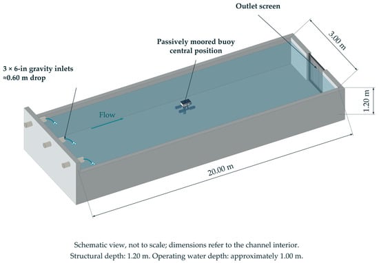
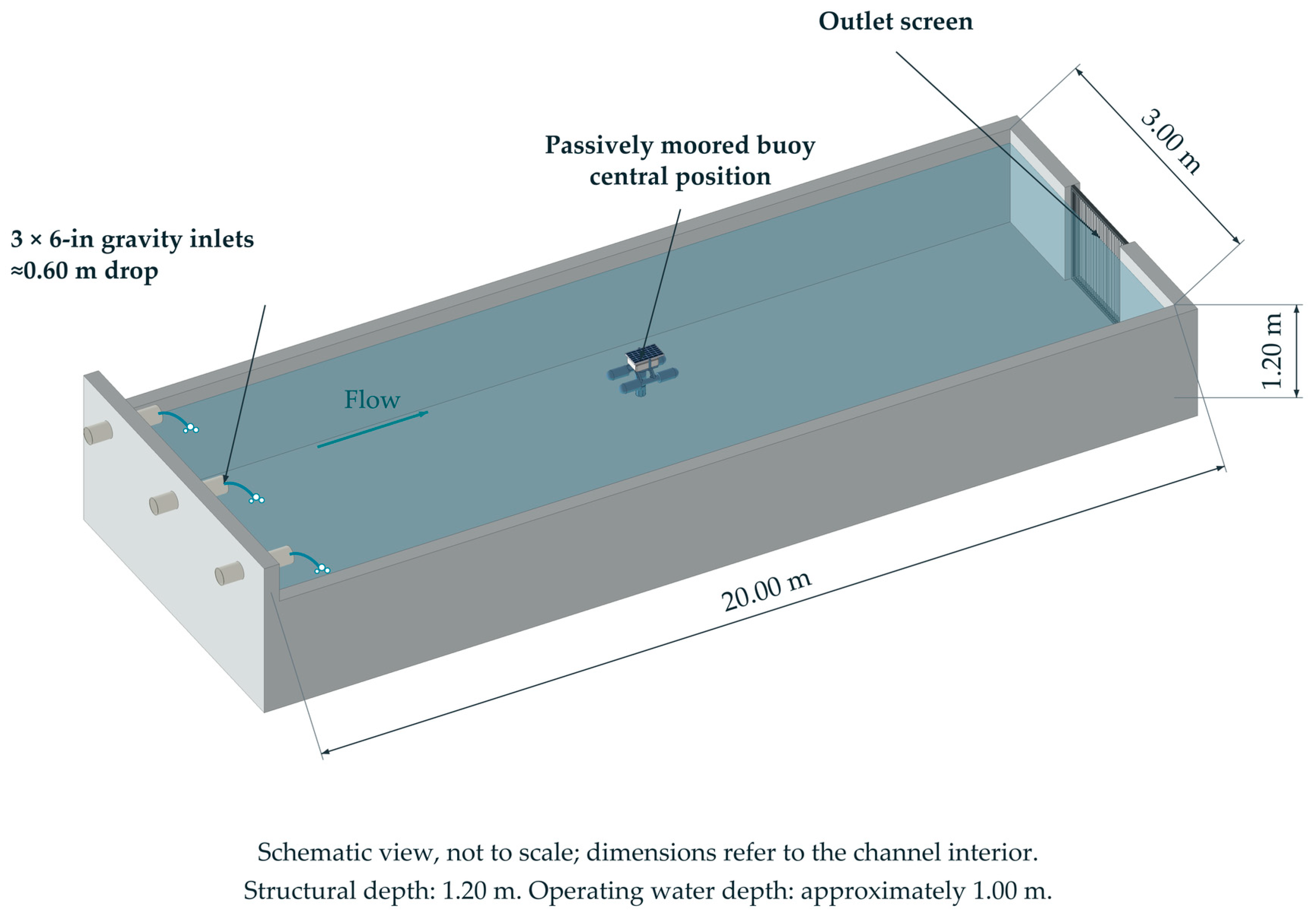
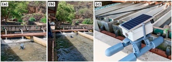
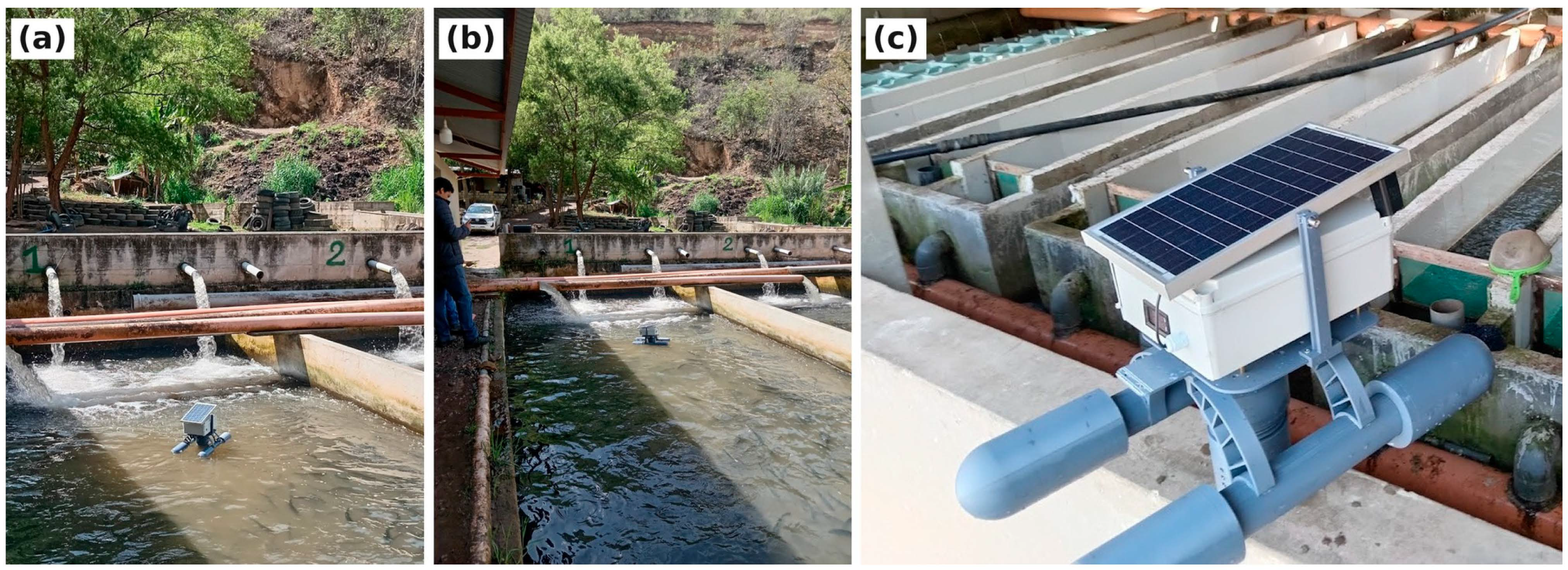
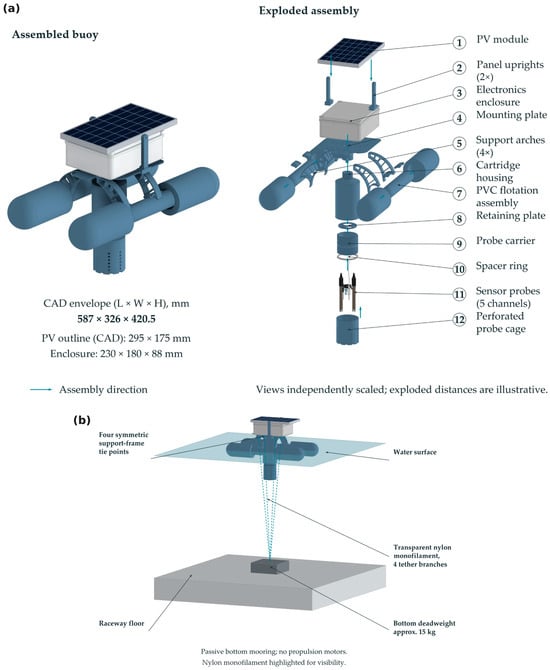
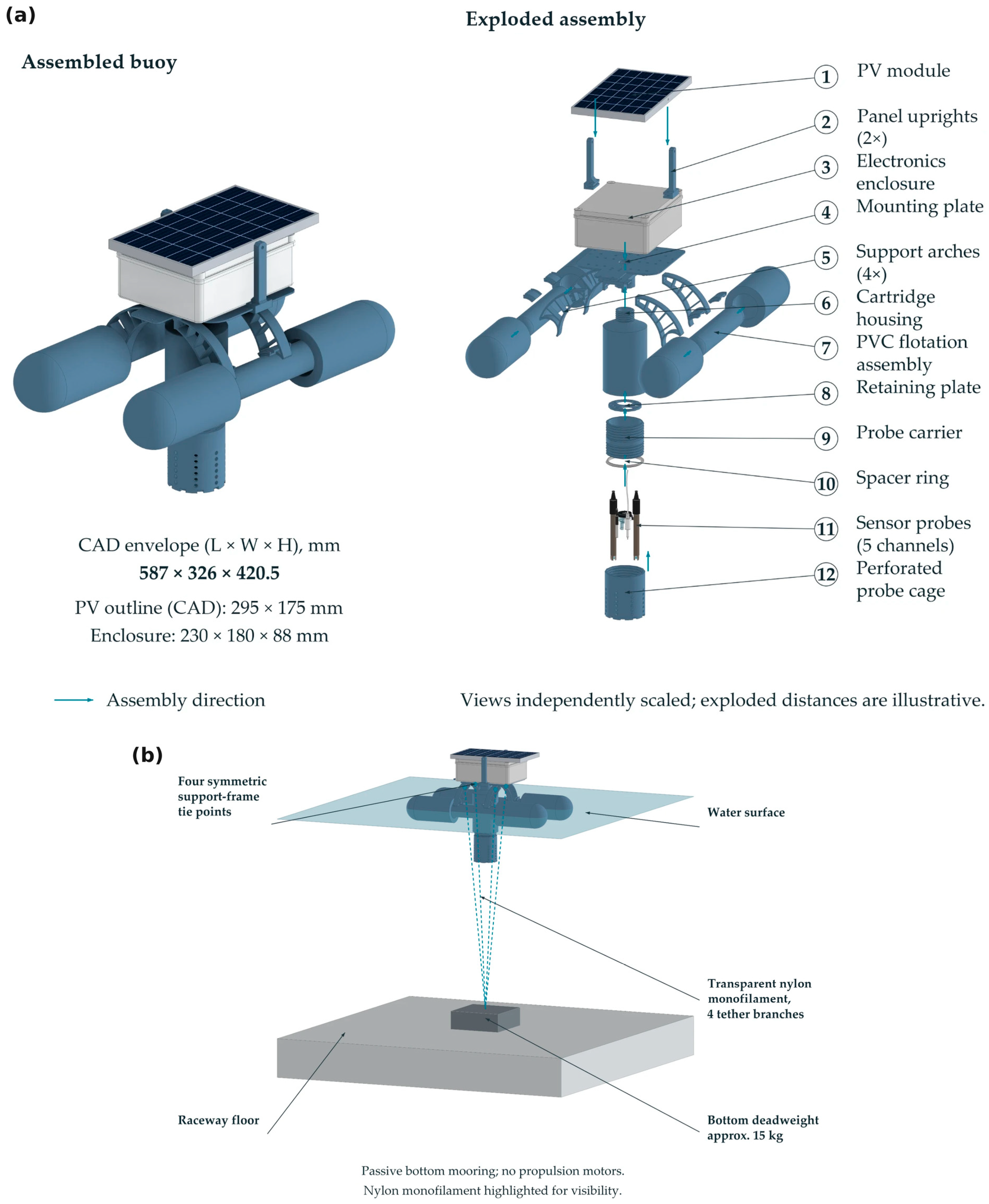
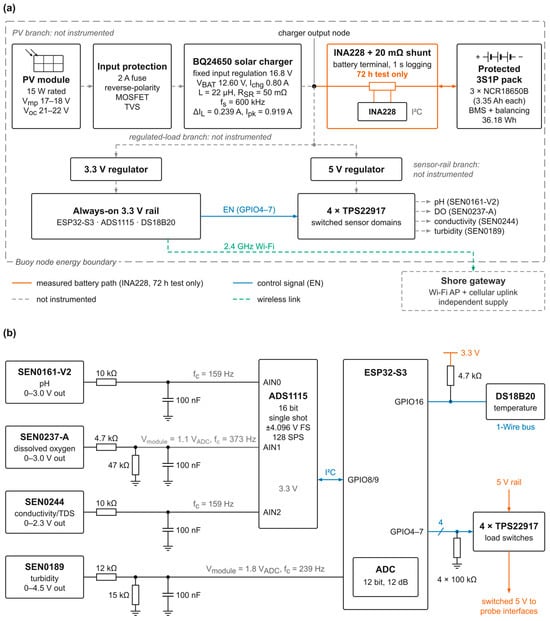
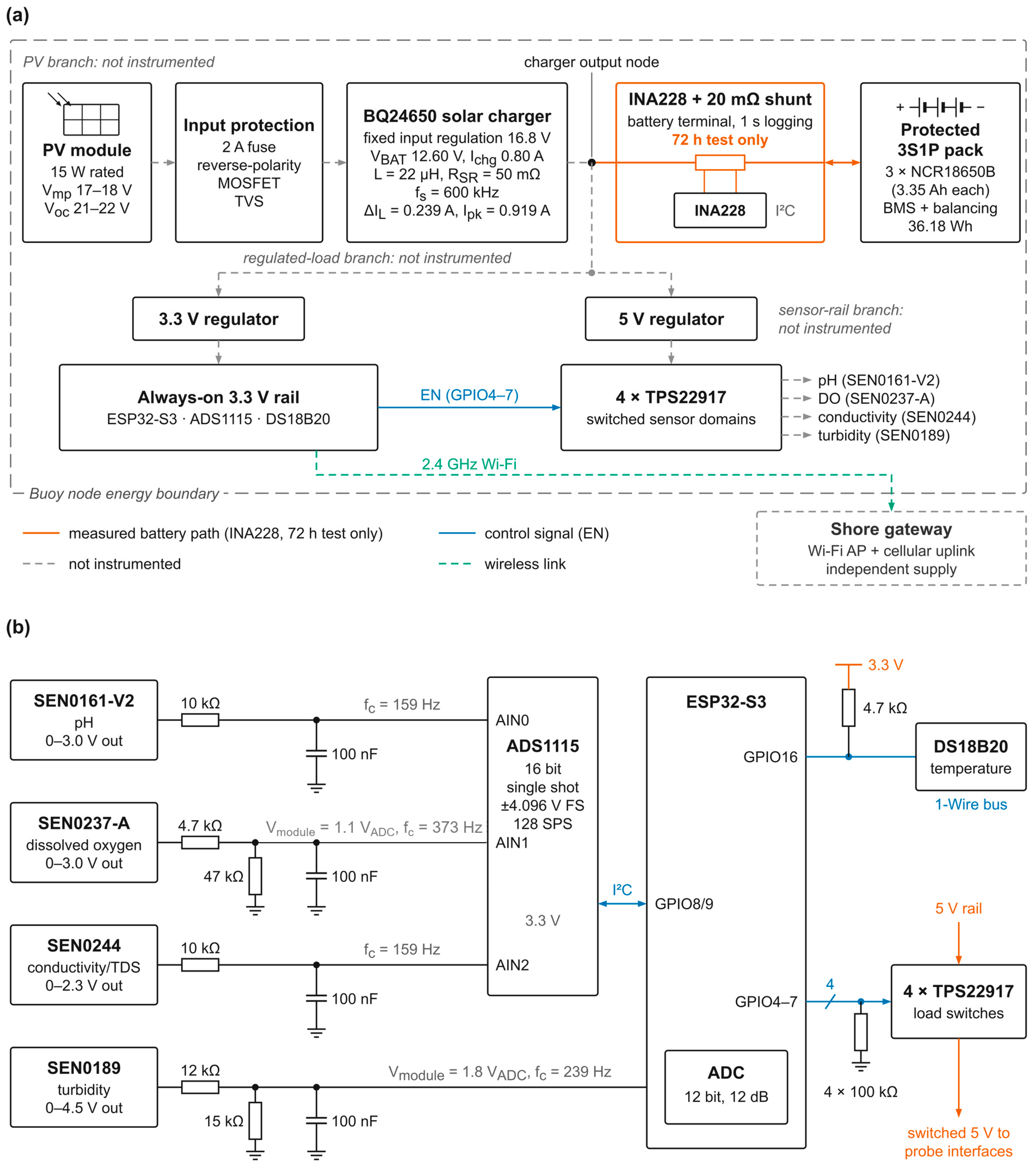
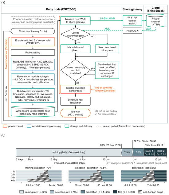
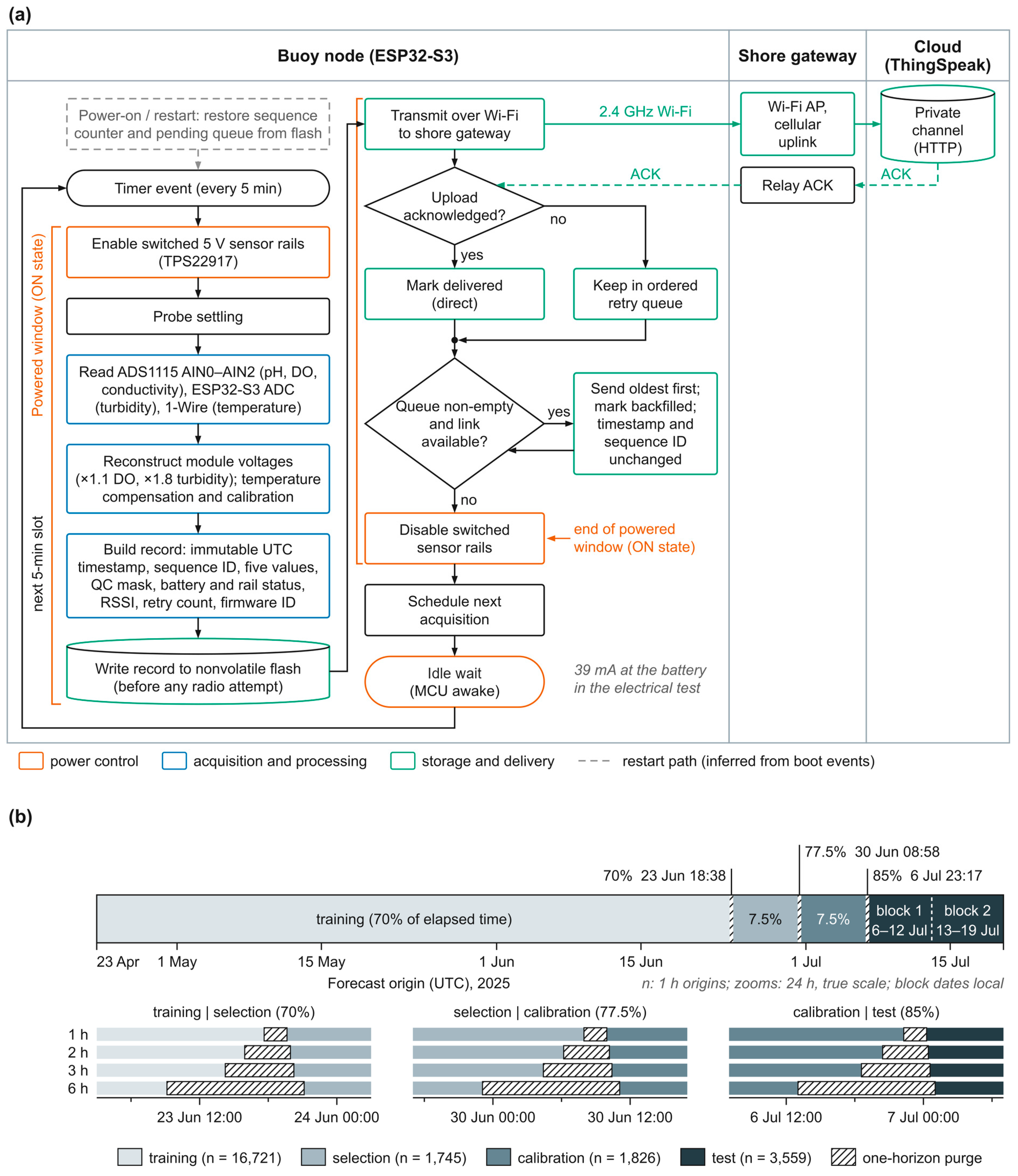
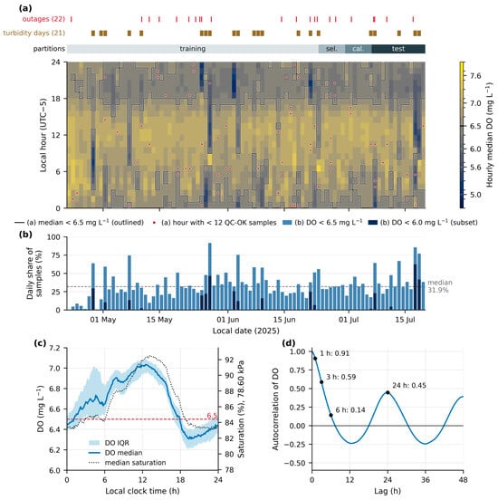
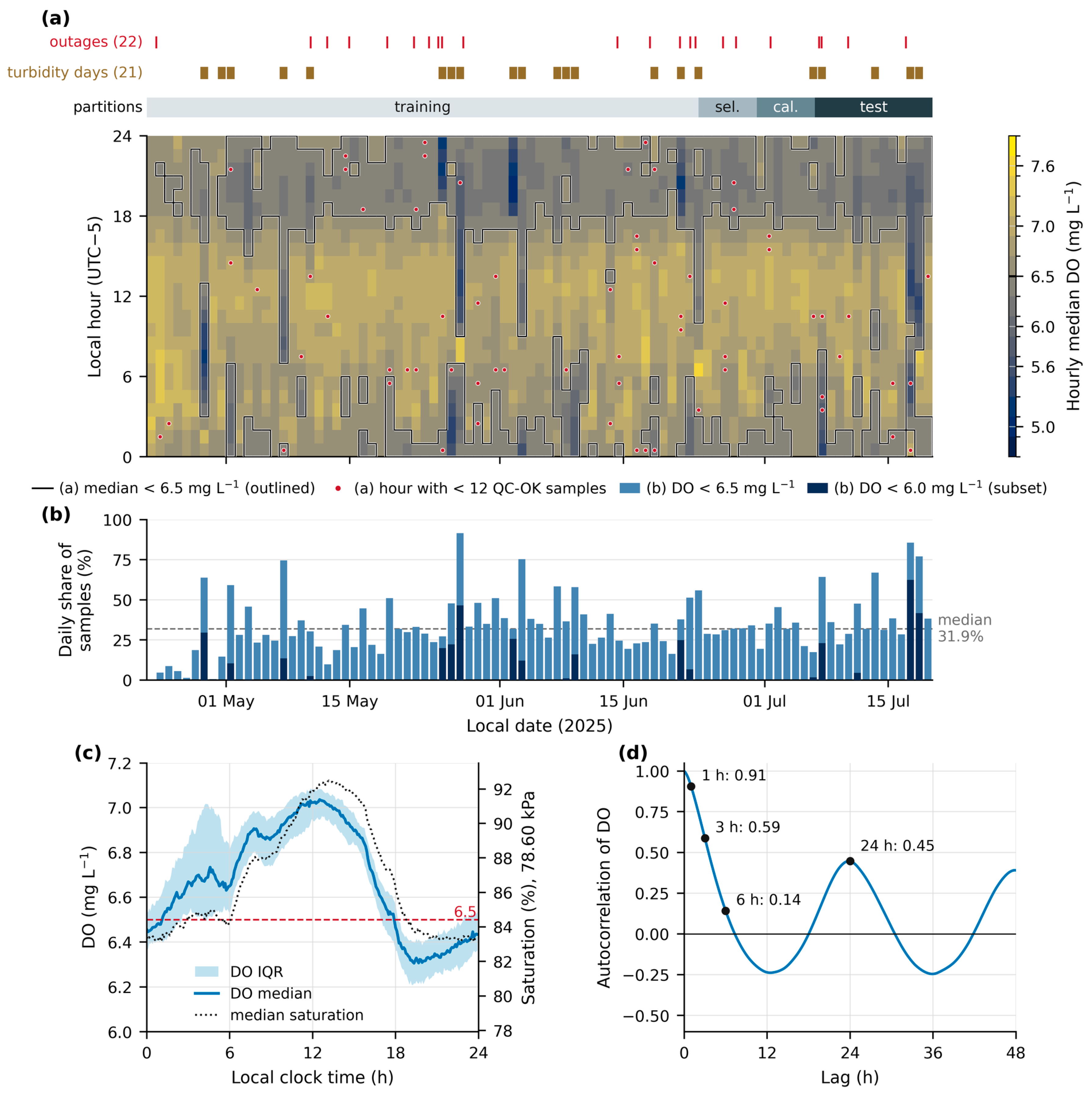
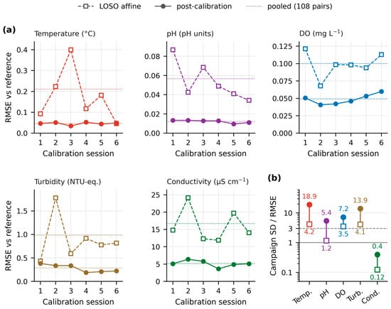
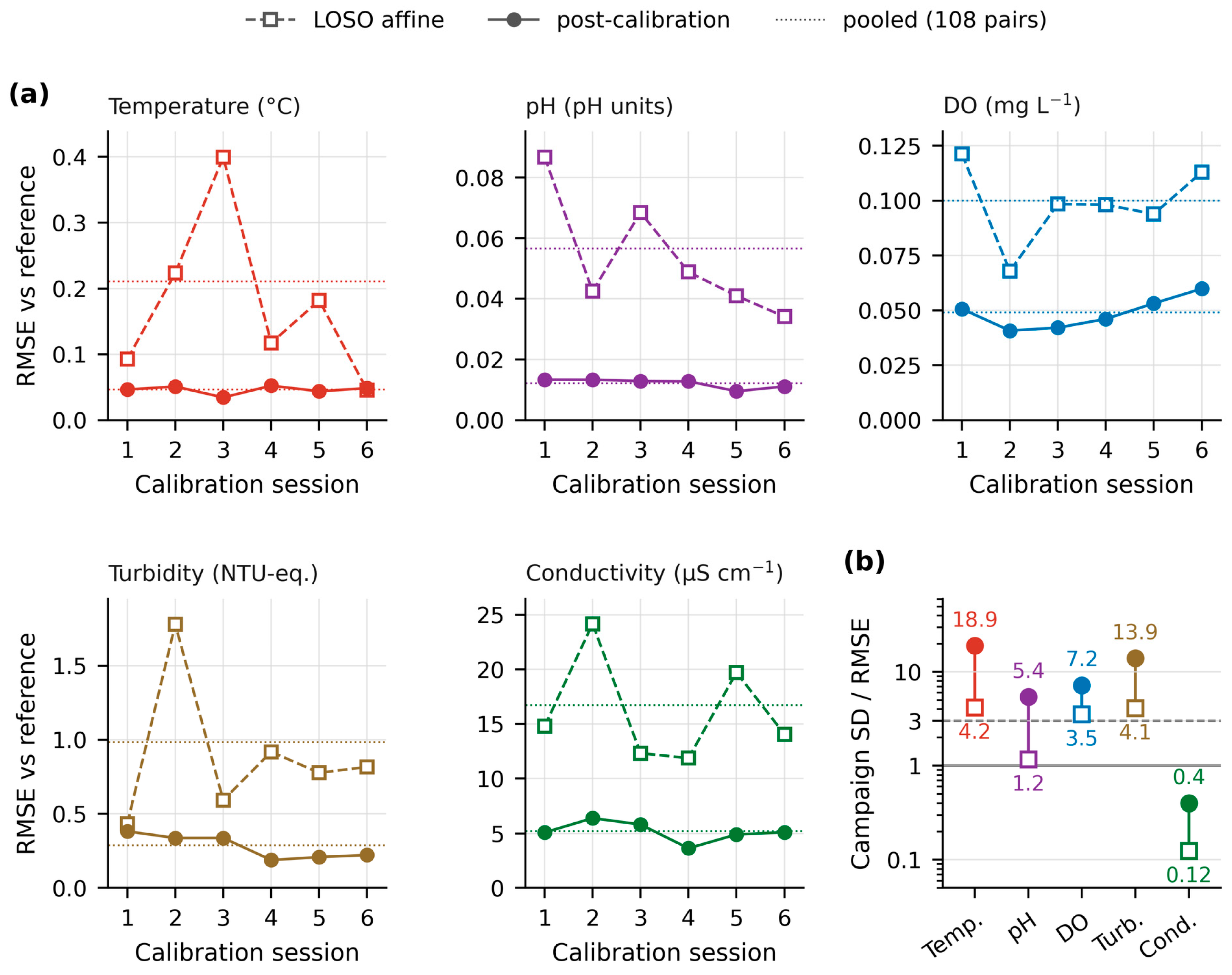
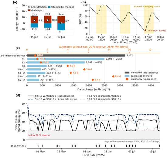
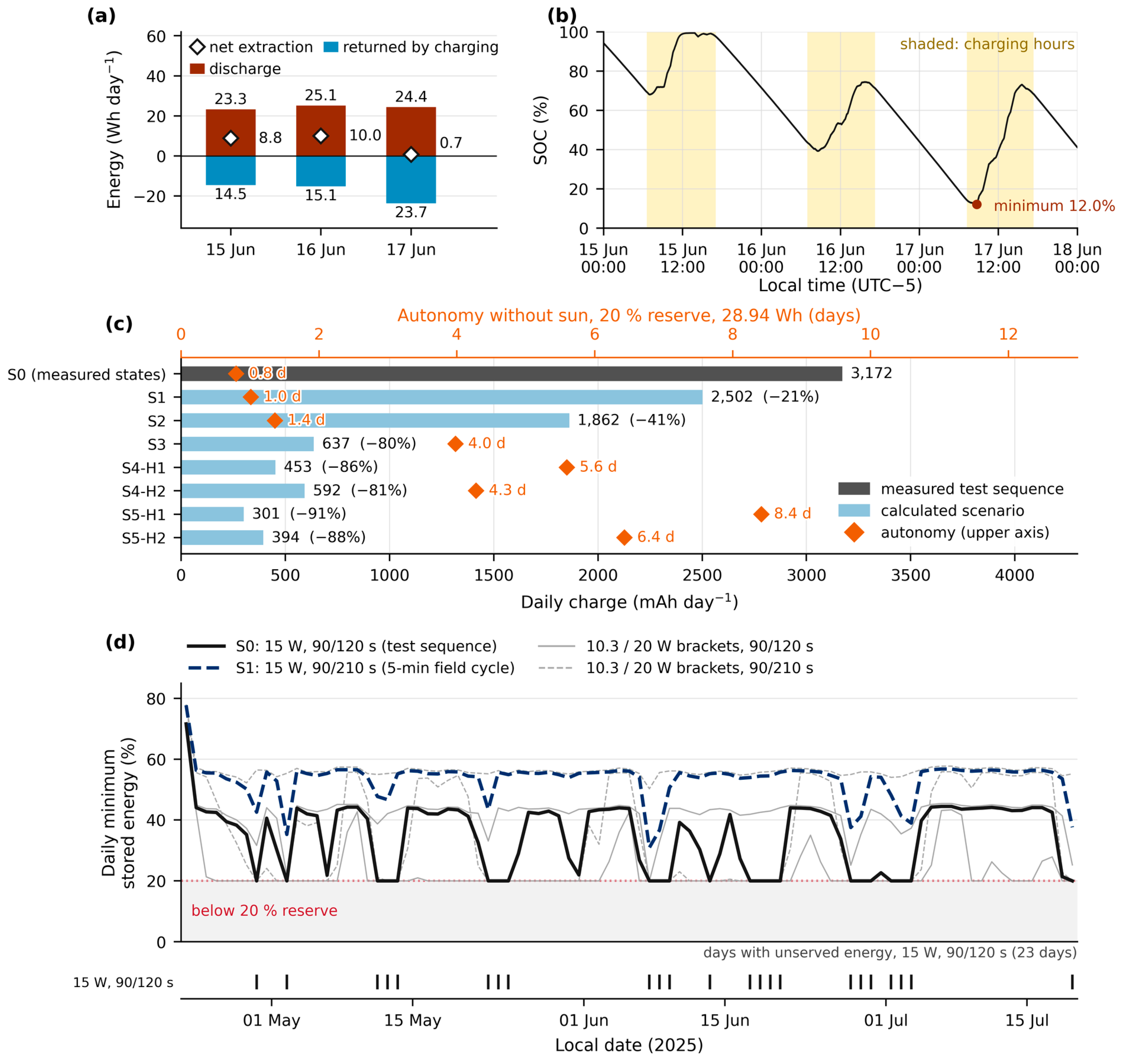
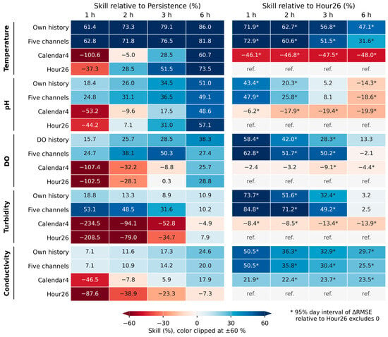
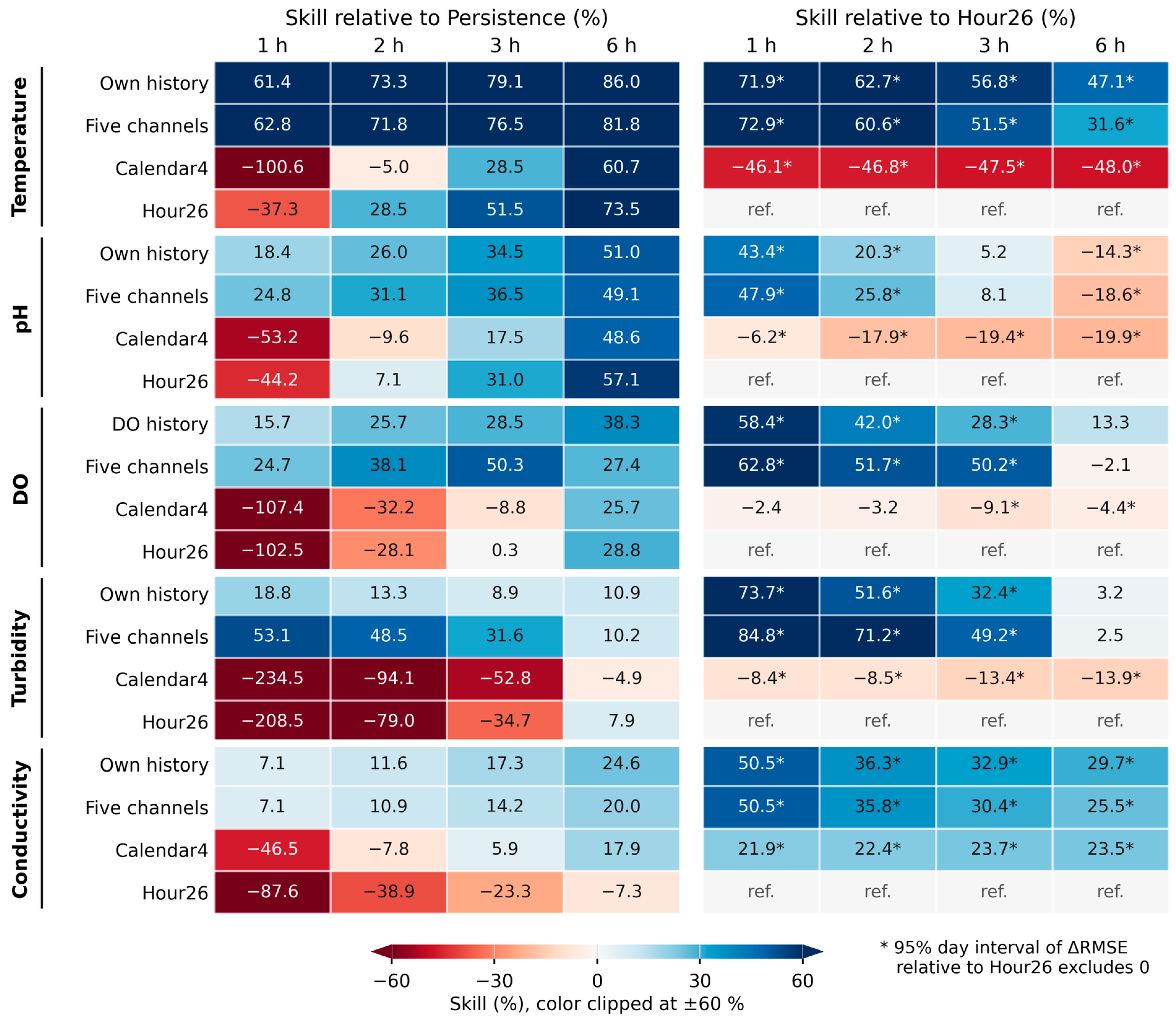
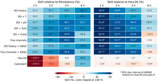
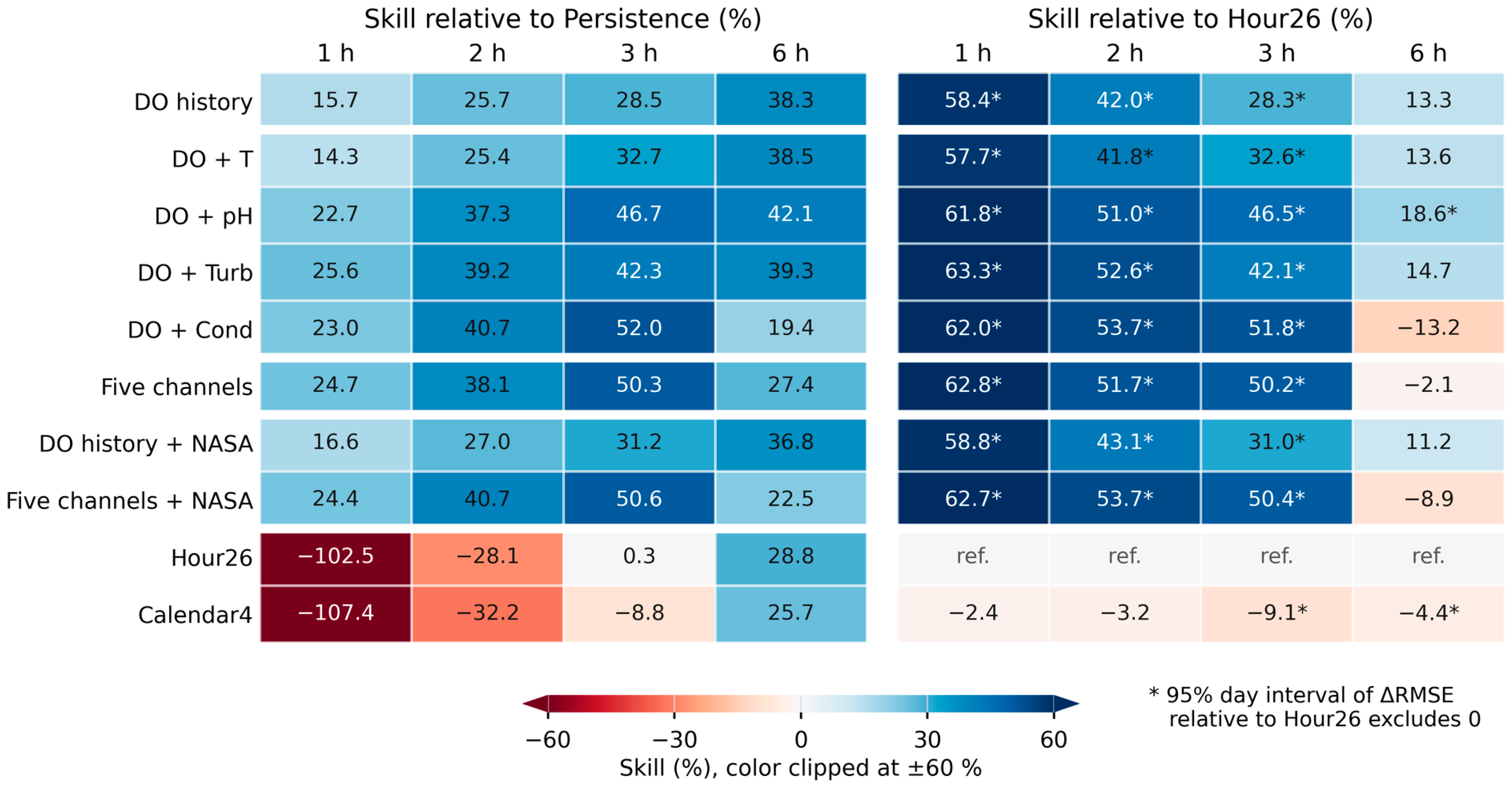
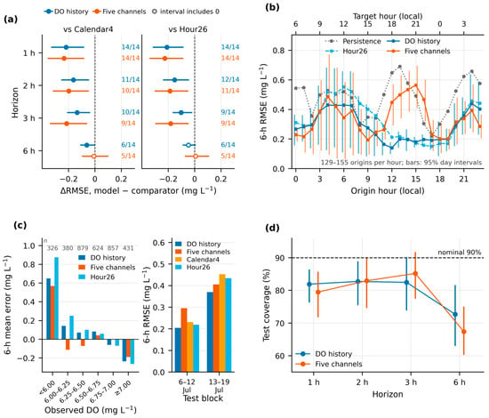
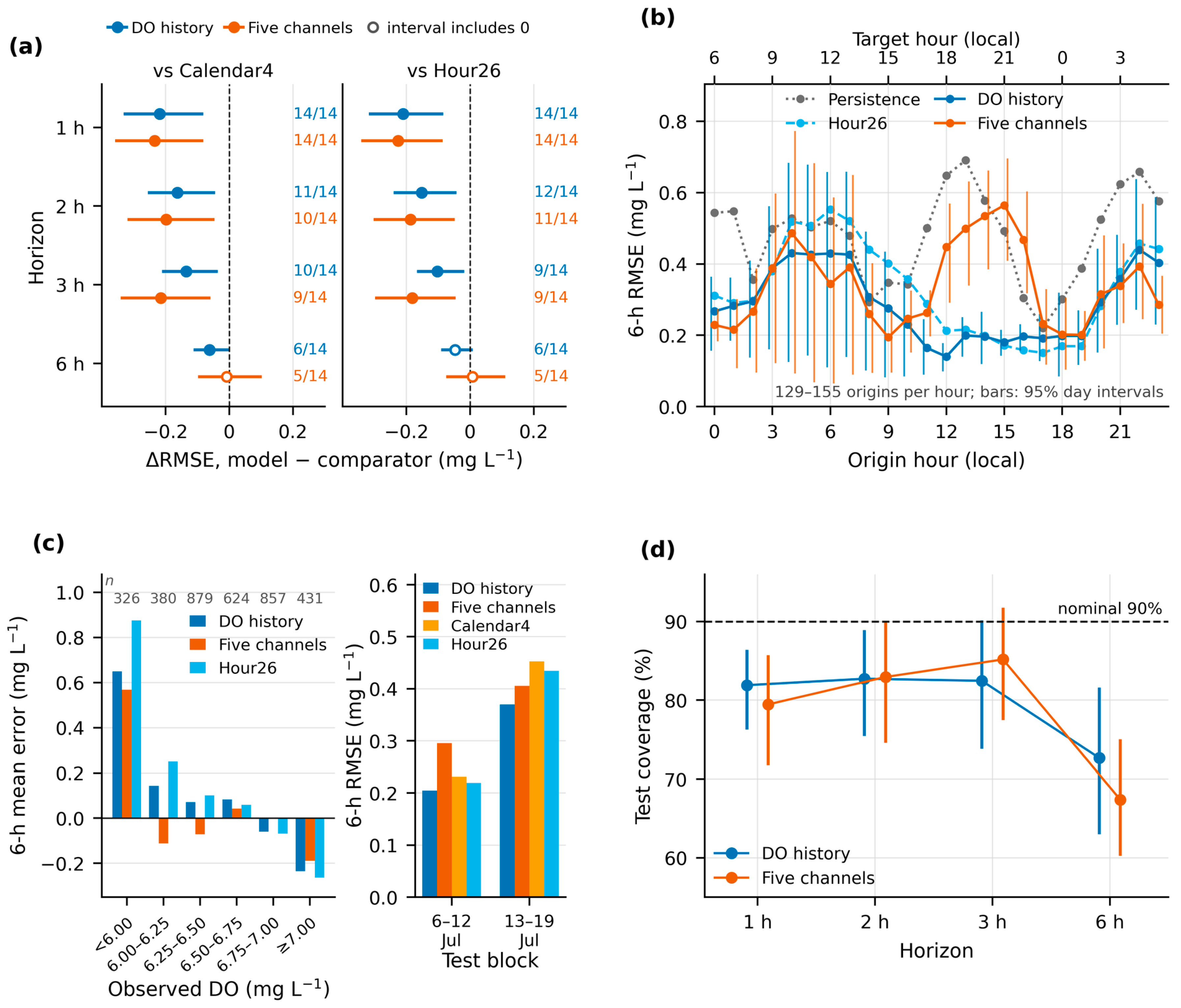
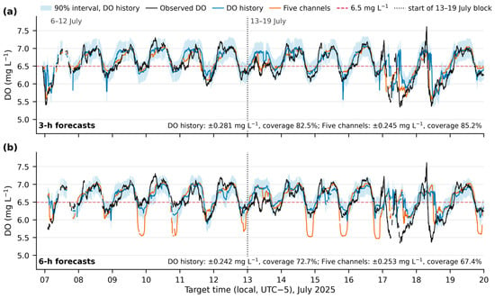
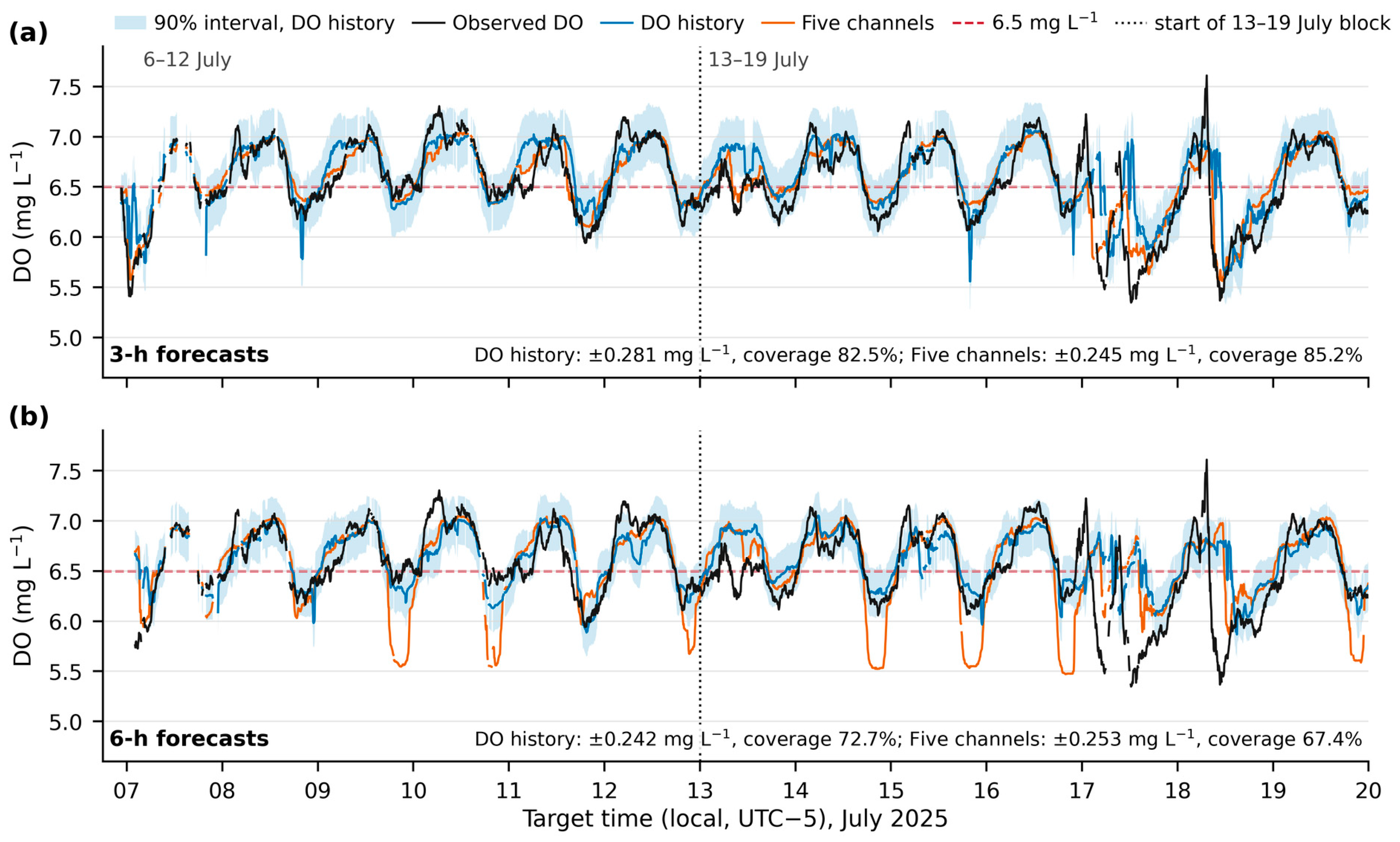
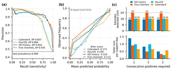
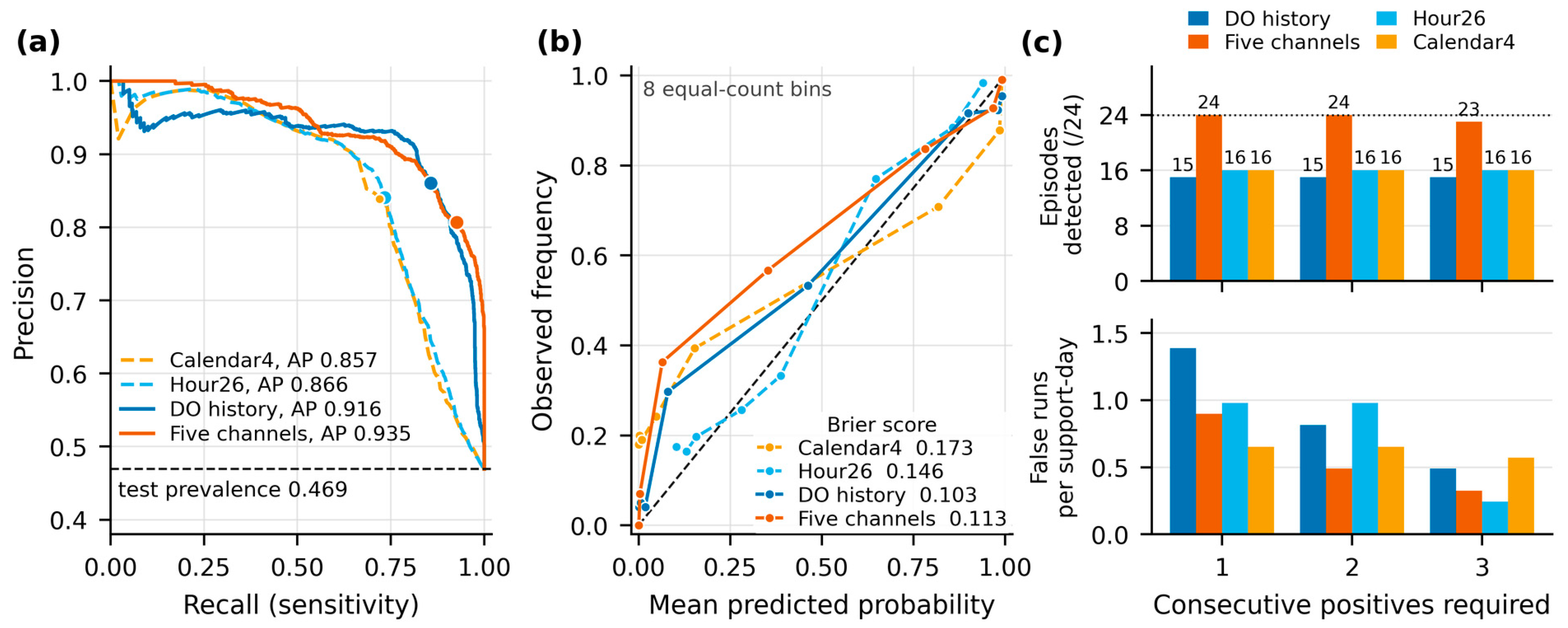

Disclaimer/Publisher’s Note: The statements, opinions and data contained in all publications are solely those of the individual author(s) and contributor(s) and not of MDPI and/or the editor(s). MDPI and/or the editor(s) disclaim responsibility for any injury to people or property resulting from any ideas, methods, instructions or products referred to in the content. |
© 2026 by the authors. Licensee MDPI, Basel, Switzerland. This article is an open access article distributed under the terms and conditions of the Creative Commons Attribution (CC BY) license.