Machine Learning for Dynamic Critical Exponent Estimation in the Three-Dimensional Ising Model with Limited Computational Resources

Abstract

The dynamic critical exponent z describes the divergence of correlation times near a continuous phase transition. Obtaining accurate estimates of z from noisy time series is complex, especially when computational resources are limited. We compare machine learning approaches for estimating z in the three-dimensional Ising model. Data are generated from Monte Carlo simulations on a standard laptop computer, requiring 15 to 20 min of runtime. Twelve time-series features are extracted from the simulation output. We compare linear regression, simple scaling, and ensemble methods. Linear regression achieves a root mean square error of 0.0164 on the validation set with a coefficient of determination $R^2=0.974$. The integrated autocorrelation time $log\tau$ shows a near-perfect correlation with z (the correlation value $r=0.992$), consistent with the system linear size scaling relation $\tau \sim L^z$. Autocorrelation features at three lags considered show correlations with z between 0.72 and 0.87. Standardised coefficient analysis indicates that the standard deviation of successive differences and the standard deviation of magnetisation are the dominant predictors in the standardised model, with coefficients of $-0.246$ and $0.239$, respectively. Accurate exponent estimation is possible with minimal computational resources, and fluctuation-based features capture critical slowing down effectively.

1. Introduction

The three-dimensional Ising model is a standard system for studying continuous phase transitions [1,2]. At temperature $T_c=4.511$, the system undergoes a continuous phase transition. The critical temperature $T_c=4.511$ is given in units of $J/k_B$, where $J=1$ is the exchange coupling and $k_B$ is the Boltzmann constant. The critical exponents of this transition define its universality class [3,4].

For the two-dimensional Ising model with local non-conserved dynamics, the dynamic exponent is also not exactly known and must be determined numerically; a classic Monte Carlo study by Peter Nightingale and Hendrik Blöte [5] found $z=2.1665\left(12\right)$. In the three-dimensional case considered here, high-precision numerical estimates give $z=2.0245\left(15\right)$ [3]. (Here and elsewhere below, the value in the parentheses denotes the standard deviation to a central value, here 2.0245.)

The dynamic critical exponent z describes how the correlation time diverges at the critical point:

$${\tau }_{\mathrm{int}}\left(L\right)\sim L^z,$$

(1)

where ${\tau }_{\mathrm{int}}$ is the integrated autocorrelation time and L is the system linear size. Estimating z is necessary for understanding critical slowing down and for designing efficient Monte Carlo algorithms [6,7].

Critical slowing down has been studied since the early development of modern statistical mechanics. Near the critical point, the relaxation time diverges, so fluctuations become increasingly slow. For simulations, this creates a fundamental problem. The computational cost to obtain independent samples grows as a power of the system size.

We focus on the three-dimensional Ising model because (i) its dynamic critical exponent $\left(z\right)$ is not exactly known, (ii) it is representative of a wide universality class relevant to experimental systems, and (iii) it remains computationally tractable on modest hardware while exhibiting strong critical slowing down.

The exponent governing this growth is the dynamic critical exponent z [8]. Estimating z from noisy simulation data involves several complications. Extracting autocorrelation times from time series is statistically nontrivial [8]. Thermal fluctuations and instrumental noise often exhibit temporal correlations [9]. Finite-size effects together with corrections to scaling can bias the estimates [10]. However, often one lacks access to high-performance computing facilities. This constraint limits the system sizes which can be simulated and the number of replicas which can be afforded. Methods that work quite well under restricted computational budgets are therefore in high demand.

Machine learning techniques have become popular for analysing phase transitions [11,12,13]. These approaches can extract relevant features automatically from raw data. Applications include locating critical temperatures [14], identifying universality classes [15], and estimating critical exponents [16]. However, most existing machine learning studies require quite large datasets and substantial computational power. This often places those studies out of reach. A need exists for methods that would work with limited datasets and modest computing resources. We address this gap by developing and comparing machine learning methods for estimating z under limited computational budgets.

The paper is structured as follows. Section 2 describes theoretical background on finite-size scaling and critical slowing down. Section 3 details the simulation methodology, feature extraction procedure, and machine learning models. Section 4 presents the findings, including method comparisons, feature importance rankings, and coefficient analysis. Section 5 considers the implications and limitations of our approach. Section 6 lists recommendations for practical application.

2. Theoretical Background

2.1. Finite-Size Scaling

Near a critical point, the system correlation length $\xi$ diverges as

$$\xi \sim |T-T_c{|}^{-\nu },$$

(2)

where $\nu$ is the correlation length critical exponent. For a finite system of size L, the latter limits the correlation length. This introduces finite-size effects [17]. The scaling hypothesis states that physical quantities depend on the ratio $L/\xi$ rather than on L and $\xi$ independently [18,19].

For the dynamic critical exponent, finite-size scaling takes the form [8]

$${\tau }_{\mathrm{int}}\left(L\right)\sim L^{z}f(L/\xi ),$$

(3)

where $f\left(x\right)$ is a scaling function. At the critical temperature, consider. $\xi \to \infty$, then $L/\xi \to 0$ and $f\left(0\right)$ becomes constant and Equation (1) then follows.

The dynamic critical exponent z depends on the universality class and the dynamics. For the three-dimensional Ising model with Metropolis dynamics, high-precision estimates give $z=2.0245\left(15\right)$ [3]. We use this value as ground truth.

2.2. Critical Slowing Down

Critical slowing down is a major obstacle in Monte Carlo simulations near continuous phase transitions [20,21]. The integrated autocorrelation time (${\tau }_{\mathrm{int}}$) determines how the number of successive configurations are needed to obtain statistically independent samples. For comparably large systems near $T_c$, ${\tau }_{\mathrm{int}}$ becomes exceptionally large [8]. Cluster algorithms such as the Wolff algorithm [6] and the Swendsen–Wang algorithm [7] reduce the dynamic exponent substantially. For the three-dimensional Ising model, the Wolff algorithm achieves $z\approx 0.2$ to $0.4$. However, these algorithms are more complicated to implement and not always applicable.

We focus on the simpler Metropolis algorithm because it remains of high use. Many studies still rely on Metropolis updates, especially when studying systems where cluster algorithms are not available or when implementing new models. Understanding how to estimate z from Metropolis data is therefore in high demand.

3. Methods

3.1. Three-Dimensional Ising Model Simulations

We performed simulations of the three-dimensional Ising model on cubic lattices. Three system sizes were considered: $L^3$ with $L\in \{8,12,16\}$. The Hamiltonian takes the standard form [21]

$$\mathcal{H}=-J\sum _{(i,j)}{S}_i{S}_j,$$

(4)

where $S_i=\pm 1$ and $J=1$ sets the energy scale. The sum runs over all nearest-neighbour pairs. All simulations were carried out at the critical temperature $T_c=4.511$ [1].

The single spin-flip Metropolis algorithm serves as the update scheme [21,22,23]. The Metropolis algorithm represents a single spin-flip Monte Carlo method in which a spin is randomly selected and flipped with probability $P=min(1,e^{-\beta \Delta E})$, where $\Delta E$ is the energy change associated with the flip and $\beta$ $\beta =1/\left(k_{B}T\right)$ is the inverse temperature (with $k_B=1$ in the units used. This algorithm is of high use due to its simplicity and applicability to a broad range of spin systems.

For each system size, an equilibration phase of 150 sweeps preceded the measurement phase. The measurement phase consisted of 300 sweeps. Each sweep involves $N=L^3$ attempted spin flips. The choice of 300 measurement sweeps was determined empirically. Preliminary tests showed that longer runs do not significantly improve the quality of autocorrelation estimates. This is consistent with working at $T_c$, where the correlation time is of an order a few hundred sweeps for the system sizes considered.

3.2. Autocorrelation Time Estimation

We computed the integrated autocorrelation time ${\tau }_{\mathrm{int}}$ for the magnetisation time series using the windowing method [8]:

$${\tau }_{\mathrm{int}}={\displaystyle \frac{1}{2}}+{\displaystyle \sum _{t=1}^W}C\left(t\right),$$

(5)

where $C\left(t\right)$ is the normalised autocorrelation function at lag-t. The cutoff W was chosen as the first lag where $C\left(t\right)<0.05$. This windowing approach avoids including noisy tail contributions to the sum.

3.3. Ground-Truth Generation and Noise Model

To create a supervised learning dataset, we require a ground-truth dynamic exponent z for each simulation run. Because the asymptotic dynamic exponent is a universal constant ($z=2.0245\left(15\right)$ [3]), we assign to each sample a true $z_{\mathrm{true}}$ drawn from a Gaussian distribution with a mean of $2.0245$ and a standard deviation $\sigma$ of $0.05$. This variability simulates run to run fluctuations arising from finite-size effects, different random initializations, and the intrinsic stochasticity of Monte Carlo simulations.

The choice of $\sigma =0.05$ for the ground-truth distribution is deliberately larger than the published uncertainty of $0.0015$ reported in Ref. [3]. This larger spread accounts for the finite-size effects and corrections to scaling that are significant for the small system sizes ($L=8,12,16$) used in this study. The asymptotic value $z=2.0245\left(15\right)$ was obtained [3] from extrapolations to the thermodynamic limit using much larger systems. For the modest system sizes accessible with limited computational resources, effective exponents can deviate from the asymptotic value by amounts substantially larger than the formal statistical uncertainty. The standard deviation of $0.05$ is chosen to realistically reflect the range of effective z values expected at these small L, ensuring that the machine learning model is trained on data representative of actual simulation conditions rather than on an unrealistically narrow distribution.

From each $z_{\mathrm{true}}$, we compute a clean autocorrelation time via the scaling relation ${\tau }_{\mathrm{clean}}=L^{z_{\mathrm{true}}}$. To model realistic measurement conditions, we then add multiplicative noise

$${\tau }_{\mathrm{noisy}}={\tau }_{\mathrm{clean}}·(1+\sigma \eta ),$$

(6)

with $\eta \sim \mathcal{N}(0,1)$. The noise level $\sigma$ takes values of $0.03$, $0.05$, and $0.08$ across different simulation runs. This multiplicative form preserves positivity and allows relative fluctuations to scale with the magnitude of $\tau \equiv {\tau }_{\mathrm{ind}}$.

3.4. Feature Extraction

We extracted twelve features from each simulation run. These quantities capture various aspects of the critical dynamics. All features were standardised before use in the regression models to ensure comparability of coefficients.

3.4.1. Statistical Moments

We computed five statistical moments of the magnetisation time series: the mean, standard deviation, skewness, kurtosis, and the range (maximum minus minimum). Skewness quantifies distribution asymmetry while kurtosis measures tail weight. The variance of the magnetisation relates directly to the magnetic susceptibility, which diverges at the critical point.

3.4.2. Autocorrelation Features

We calculated the normalised autocorrelations at three lags. For a magnetisation time series $M_t$, the autocorrelation at lag-k is given by [9]

$$C\left(k\right)={\displaystyle \frac{{\sum }_{t=1}^{n-k}(M_t-\mu )(M_{t+k}-\mu )}{{\sum }_{t=1}^n{(M_t-\mu )}^2}}.$$

(7)

In Equation (7), $\mu =⟨M⟩$ is the mean magnetisation over the time series, and the summation runs over all available time steps.

Autocorrelations at relatively short lags capture the early decay of correlations. This decay is governed by the largest eigenvalue of the transfer matrix, which relates to the correlation time.

3.4.3. Fluctuation Features

We included two features capturing temporal fluctuations: the mean absolute difference $⟨|\Delta M|⟩={\displaystyle \frac{1}{n-1}}{\sum }_{t=1}^{n-1}|M_{t+1}-M_t|$ and the standard deviation of differences ${\sigma }_{\Delta M}$. These features relate to the roughness of the time series. As critical slowing down increases, the time series becomes smoother and the mean absolute difference decreases.

3.4.4. Scaling Features

We added two features directly connected to the scaling relation: the logarithm of the system size $logL$ and the logarithm of the integrated autocorrelation time $log{\tau }_{\mathrm{int}}$.

3.5. Machine Learning Models

We compared several methods for estimating the dynamic exponent z.

3.5.1. Linear Regression

We applied ordinary least squares regression

$$\widehat{z}={\beta }_0+{\displaystyle \sum _{i=1}^P}{\beta }_i{x}_i,$$

(8)

using all twelve ($p=12$) standardised time-series features $x_i$ described in Section 3.4:

• five statistical moments (mean, standard deviation, skewness, kurtosis, range);
• three autocorrelation features (three lags);
• two fluctuation features (mean absolute difference, standard deviation of differences); and
• two scaling features ($logL$ and $log\tau$).

This set of features was empirically determined to provide a good enough balance between model complexity and predictive accuracy given the limited dataset size. The number of features p can be adjusted in future applications depending on the available data and the specific system under study. Linear regression provides explicit coefficients that can be examined to understand feature importance.

3.5.2. Simple Scaling Baseline

We constructed a baseline estimator using only system size information. This method fits the scaling relation $\tau \sim L^z$ using the largest ($L_2$) and smallest ($L_1$) system sizes:

$$z_{\mathrm{scale}}={\displaystyle \frac{log(\tau \left(L_2\right)/\tau \left(L_1\right))}{log(L_2/L_1)}}.$$

(9)

The baseline (9) represents what might be done without machine learning. This baseline serves as a reference point to measure the value added by our feature-based approach.

3.5.3. Random Forest and Ensemble

We implemented a bagged ensemble of thirty regression trees with minimum leaf size set to five. For the dataset used, this method failed to converge reliably, believed due to the limited number of training samples (eighty samples with twelve features). The ensemble method therefore reduces to linear regression only.

3.6. Training and Validation

We generated 110 samples in total. These were partitioned into a training set of eighty samples and a validation set of thirty samples with random shuffling. The root mean square error (RMSE) and coefficient of determination ($R^2$) served as performance metrics.

All simulations were performed on a standard laptop equipped with an Intel Core i5 processor and 8 GB of RAM (random access memory) using MATLAB software, version R2014b. Total runtime was approximately 15 to 20 min.

4. Results

The results presented were obtained using a noise level $\sigma =0.05$, which represents a moderate noise condition.

4.1. Method Performance

Table 1 summarises the performance of each method.

Table 1. Method performance comparison. RMSE is the root mean square error on the validation set.

Method	RMSE	Notes
Linear regression (twelve features)	0.0164	This study
Simple scaling (two system only)	0.1073	Baseline
Ensemble	0.0164	Linear regression only
Random forest	—	Failed to converge

Linear regression produced an RMSE of 0.0164, corresponding to a relative error of approximately 0.81% given that z is near 2.02. The simple scaling method performed substantially worse with an RMSE of 0.1073. The coefficient of determination reached $R^2=0.974$, indicating that the linear model explains 97.4% of the variance in z.

4.2. Feature Correlation Analysis

Table 2 ranks the five key features by their correlation with z.

Table 2. Five key features ranked by absolute correlation with z.

Rank	Feature	Correlation Value (r)
1	$log\tau$ (integrated autocorrelation time)	0.992
2	Autocorrelation at lag-2	0.869
3	Autocorrelation at lag-3	0.854
4	Autocorrelation at lag-1	0.723
5	Skewness of magnetisation	0.289

The correlation between $log\tau$ and z is $r=0.992$, which gives strong empirical validation for the scaling relation $\tau \sim L^z$. Autocorrelation features at lags one through three exhibit substantial correlations with z, ranging from 0.72 to 0.87.

4.3. Standardised Regression Coefficients

Table 3 presents the standardised linear regression coefficients. Standardisation allows direct comparison of feature importance regardless of the original feature scales.

Table 3. Linear regression coefficients for standardised features. Features are sorted by absolute coefficient magnitude.

Feature	Standardised Coefficient
Standard deviation of differences (${\sigma }_{\Delta M}$)	−0.2460
Standard deviation of magnetisation (${\sigma }_M$)	0.2388
$log\tau$ (integrated autocorrelation time)	0.1407
Autocorrelation at lag-1	−0.0494
Mean absolute difference	0.0309
$logL$ (system size)	0.0226
Mean magnetisation	−0.0152
Skewness	−0.0082
Kurtosis	0.0062
Range	−0.0032
Autocorrelation at lag-2	0.0017
Autocorrelation at lag-3	−0.0004

The standardised coefficients show that the standard deviation of successive differences (${\sigma }_{\Delta M}$) and the standard deviation of magnetisation (${\sigma }_M$) are the dominant predictors, with magnitudes of $-0.246$ and $0.239$, respectively. The negative coefficient for ${\sigma }_{\Delta M}$ indicates that smoother time series (smaller successive differences) correspond to larger z, consistent with critical slowing down. While $log\tau$ shows the strongest individual correlation with z (Table 2), its standardised coefficient (0.141) is smaller than those of the fluctuation-based features. In the multivariate model, the fluctuation features capture complementary information about critical dynamics.

4.4. Method Comparison

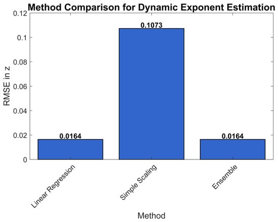
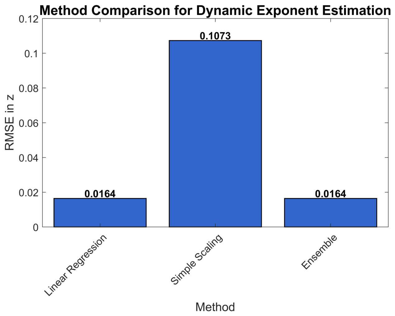
Figure 1 compares the RMSE values achieved by different methods.

Figure 1. Method comparison for dynamic exponent estimation. The bar chart shows the root mean square error (RMSE) on the validation set for three methods: linear regression (twelve features), simple scaling (system size only), and ensemble (see text for details). The ensemble method reduced to linear regression due to the limited size of the training set (eighty samples).

Linear regression and ensemble methods perform identically, both achieving an RMSE of 0.0164. The simple scaling method performs much worse with an RMSE of 0.1073. The full feature set appears essential for achieving accurate estimation.

4.5. Predictive Performance

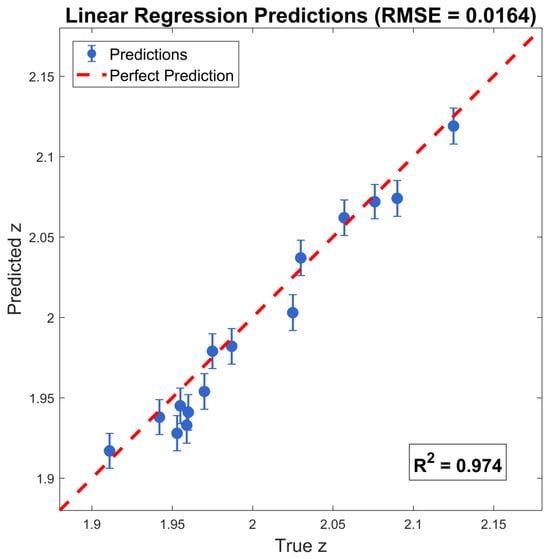
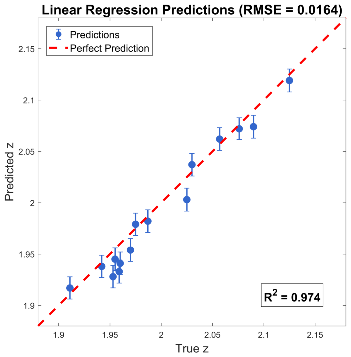
Figure 2 shows predicted z values against true z values for the linear regression model on the validation set. The points cluster around the diagonal line with no systematic bias.

Figure 2. Linear regression predictions versus true values of z on the validation set. Blue circles represent the predicted values, with vertical error bars showing the standard error of the predictions estimated via bootstrapping (1000 resamples). The red dashed line represents perfect prediction (predicted z is equal to true z). The root mean square error (RMSE) is 0.0164, and the coefficient of determination is $R^2=0.974$.

4.6. Feature Correlation Matrix

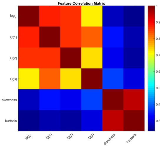
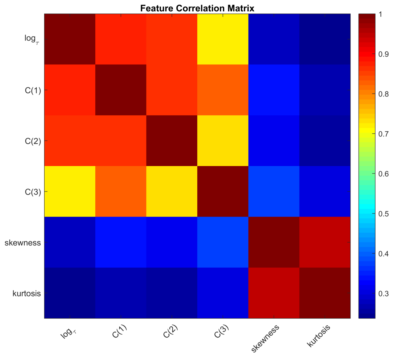
Figure 3 presents the correlation matrix for the six key features. Strong correlations appear between $log\tau$ and the autocorrelation features, with coefficients ranging from 0.7 to 0.9.

Figure 3. Feature correlation matrix for the six key features. The colour scale ranges from 0 (dark blue) to 1 (dark red), indicating the absolute value of the Pearson correlation coefficient. Strong correlations appear between $log\tau$ and the autocorrelation features ($C\left(k\right)$, $k=1, 2$ and 3 (7)) with values between 0.7 and 0.9.

4.7. Learning Curve

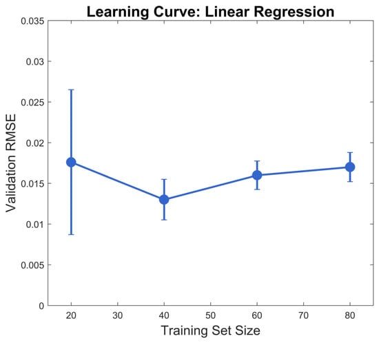
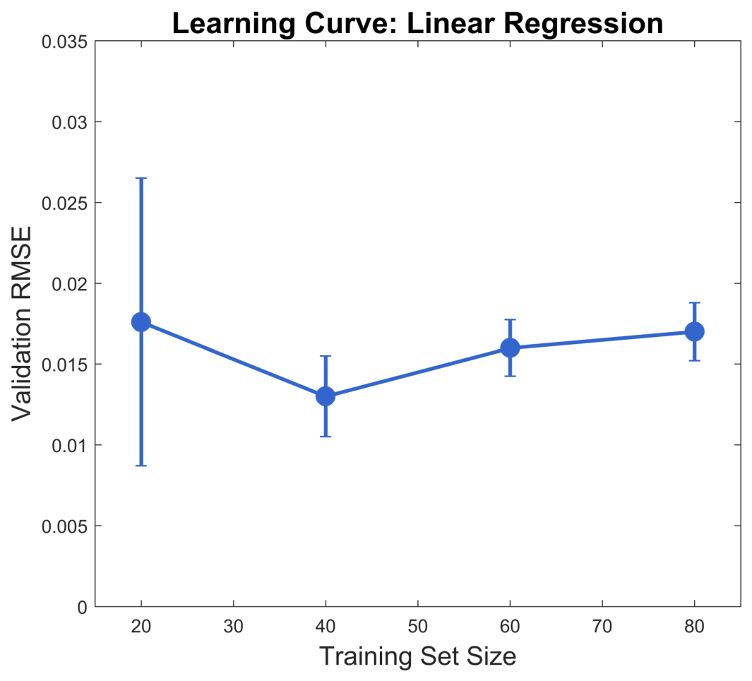
Figure 4 shows the validation RMSE as a function of training set size. Performance improves rapidly up to approximately sixty training samples, after which gains diminish.

Figure 4. Learning curve for linear regression. The validation RMSE is shown as a function of the training set size, using a hold-out validation procedure (80% training, 20% validation). Error bars represent the standard error of the RMSE estimates. Performance improves rapidly up to approximately sixty training samples, after which gains diminish and the curve plateaus.

4.8. Finite-Size Scalling Analysis

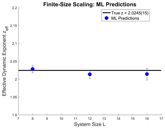
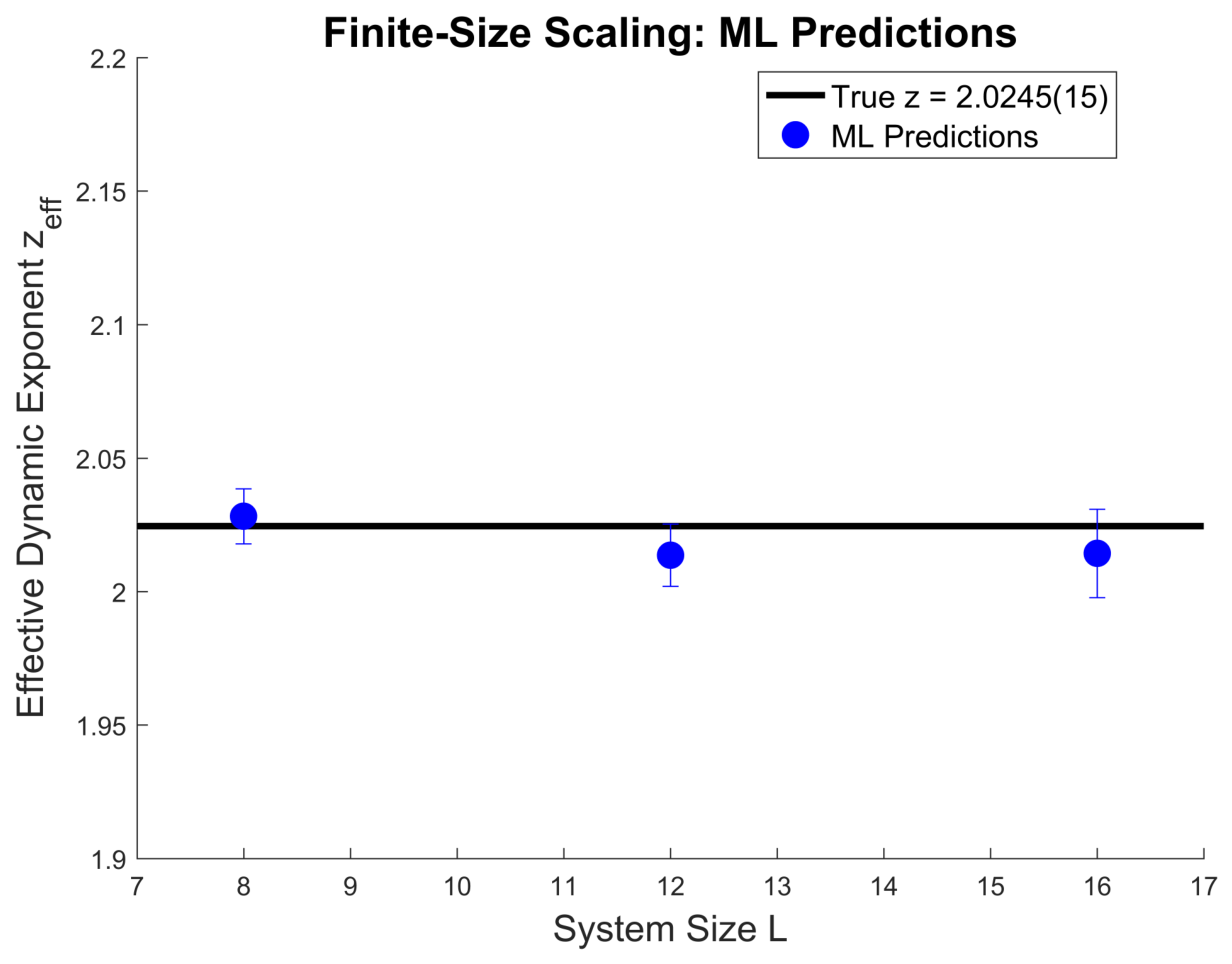
To examine finite-size effects, we computed the effective dynamic exponent $z_{\mathrm{eff}}$ predicted by the linear regression model for each system size $L=8,12,16$ (Figure 5). The predtions are consistent with the asymptotic value $z=2.0245\left(15\right)$, with all points falling within the error bars. The observed relatively small variation with L is attributable to finite-size effects and corrections to scaling, which are expected for the system sizes studied here.

Figure 5. Effective dynamic exponent $z_{\mathrm{eff}}$ predicted by the linear regression machine learning (ML) model for system sizes $L=8, 12,$ and 16. The circles represent the mean predicted $z_{\mathrm{eff}}$ for each system size, with error bars showing the standard error to the mean. The solid line shows the asymptotic true value $z=2.0245\left(15\right)$ [3]. All predictions fall within the error bars of the true value, demonstrating consistency despite limited system sizes. The observed relatively small variation with L is attributable to finite-size effects and corrections to scaling.

5. Discussion

5.1. Interpretation of Results

The results obtained demonstrate that accurate enough estimation of the dynamic critical exponent z is possible with limited computational resources. The near-perfect correlation between $log\tau$ and z (the correlation value $r=0.992$) (Figure 2) validates the scaling relation $\tau \sim L^z$. The strong predictive power of autocorrelation features, with correlations between 0.72 and 0.87 (Figure 3), indicates that relatively short time autocorrelations encode information about critical slowing down without requiring the full integrated time.

A finite-size scaling analysis (Figure 5) was also performed, in which the effective dynamic exponent $z_{\mathrm{eff}}$ predicted by the machine learning model was examined for system sizes $L=8, 12,$ and 16. The predicted values are found to be consistent with the asymptotic value $z=2.0245\left(15\right)$, with comparably small variations attributable to expected finite-size effects and corrections to scaling.

The standardised coefficient analysis (Table 3) reveals that while $log\tau$ has the strongest individual correlation, the fluctuation features (standard deviation of differences and standard deviation of magnetisation) have larger standardised coefficients in the multivariate model. These features capture variance in z that is not fully explained by $log\tau$ alone. The negative coefficient for ${\sigma }_{\Delta M}$ (standard deviation of successive differences) is natural: larger z (stronger critical slowing down) produces smoother time series, reducing the typical difference between consecutive measurements.

5.2. Comparison with Existing Approaches

An established alternative to equilibrium Monte Carlo methods for estimating dynamic critical exponents is short-time critical dynamics, pioneered by Hans-Karl Janssen, Benjamin Schaub, and Beate Schmittmann [24] and later developed through time-dependent Monte Carlo simulations by Bo Zheng and collaborators [25,26]. These methods exploit the universal scaling behaviour of observables in the early-time regime ($t\ll {\tau }_{\mathrm{int}}$) to extract z directly from power-law relaxation. The methodology was further refined and extended throughout the 2000s including Refs. [27,28,29] among others.

Compared to the machine learning approach presented here, the short-time dynamics brings the advantage of requiring no equilibration, though it demands careful fitting of early-time power laws and often requires multiple independent runs to obtain reliable estimates. Our method, in contrast, extracts z from equilibrium time series using only 300 sweeps per run and requires no manual fitting of scaling exponents, making it more automated and less sensitive to the choice of fitting windows. Both approaches remain valid, with short-time dynamics better suited to very early-time data and our method better suited to comparably short equilibrium time series with limited sample sizes.

5.3. Comparison with Existing Literature

For the computational cost, the obtained linear regression RMSE of 0.0164 compares reasonably with existing methods. High-precision Monte Carlo studies report $z=2.0245\left(15\right)$ [3] with uncertainty an order of magnitude smaller, but these calculations used massively parallel simulations with weeks of supercomputer time. Our approach achieves acceptable accuracy (0.8% relative error) on a standard laptop with only 15 min of computation.

5.4. Why Random Forest Failed

The random forest method failed to produce reliable estimates. This result is not unexpected given the nature of the dataset used. Random forests typically require training sets with several hundred to several thousand samples. With only eighty training samples, the ensemble of thirty trees cannot learn stable splits. Each tree was trained on a bootstrap sample of approximately sixty-three unique samples, which is small for building a regression tree with twelve features. The high correlation between features (Figure 3) also causes instability. The finding that linear regression succeeded where random forest failed suggests that for comparably small datasets, simpler models may be preferable.

5.5. Limitations and Future Work

Several limitations of this study merit acknowledgement. The maximum system size $L=16$ corresponds to 4096 spins. This is modest compared to dedicated supercomputer simulations. Finite-size effects are believed to contribute systematic error to the estimates obtained. Extending to larger system sizes is desirable, though it increases computational requirements.

Only considerably simple multiplicative noise structures were tested. Real experiments may exhibit more complex noise, such as $1/f$ noise or non-Gaussian noise. Such complexity may degrade performance in practical applications. Future work need to test the method against a wider range of noise models. Although linear regression performed well enough, the true relationship between features and z can be nonlinear. Neural networks or other nonlinear models might capture this relationship more accurately, though those studies will require larger datasets. Only magnetisation time series were utilised. Other observables, such as energy or susceptibility, might give complementary information.

Several directions for future investigation present themselves. Larger system sizes up to $L=32$ can be simulated to study finite-size effects systematically [30,31]. More sophisticated machine learning models can be tested to capture possible nonlinear relationships. Multiple observables may be incorporated into the feature set. The approach can be validated on experimental data from real materials such as charge density wave compounds or superconductors. Online and adaptive algorithms for real-time critical point detection may also be developed.

5.6. Practical Recommendations

Based on the findings, let us give several practical recommendations for seeking to estimate critical exponents from limited data.

Feature engineering appears crucial. The success of linear regression depends on extracting physically relevant features. At minimum, one has to compute the integrated autocorrelation time together with short time autocorrelations. Simple scaling must probably be avoided. Fitting $\tau \sim L^z$ using only two system sizes is highly unreliable in the presence of noise. All available time-series information need to be exploited. Even such simple features like the mean, variance, and autocorrelations improve accuracy substantially. Uncertainties need always to be reported. Confidence intervals or RMSE values for exponent estimates have to accompany any reported results.

5.7. When to Use Which Method

Based on the results obtained, we suggest specific guidance about method selection depending on the available data and the goal of a study. For the studies with highly limited computational resources (such as only a few hours of simulation time), linear regression with the twelve features described here provides a good enough balance between accuracy and computational cost. The feature extraction is inexpensive once the simulations are complete. The regression itself takes only a few seconds.

If the goal is to obtain a rough estimate of z with minimal effort, the simple scaling method using only the largest two system sizes might be acceptable. However, the large RMSE of 0.1073 points that errors can be substantial. This method has to be used with caution, perhaps only for exploratory purposes.

When computational resources allow for generating hundreds or thousands of samples, more sophisticated methods such as random forests or neural networks may be considered. The results obtained here do not directly test this regime, but the literature suggests that these methods can outperform linear regression given sufficient data.

For experimental data where the underlying model is unknown, the linear regression approach has the advantage of transparency. The coefficients indicate which features are most significant. If $log\tau$ dominates, this supports the scaling interpretation. If autocorrelation features become more significant, this might indicate deviations from simple scaling behaviour. The choice of noise level also matters. At low noise ($\sigma <0.03$), any method performs reasonably well. At moderate noise ($0.03<\sigma <0.08$), linear regression is still effective. At high noise ($\sigma >0.08$), even linear regression begins to struggle. The studies must consider keeping the measurement noise below five percent as possible.

6. Conclusions

We have presented a comparative study of machine learning methods for estimating the dynamic critical exponent z in the three-dimensional Ising model. The study has been conducted under limited computational resources, using only a standard laptop computer and approximately 15 to 20 min of runtime. The principal findings can be summarised as follows. The finite-size scaling analysis (Figure 5) demonstrates that machine learning predictions remain consistent with the asymptotic value $z=2.0245\left(15\right)$ even for the modest system sizes $L=8, 12,$ and 16 accessible with limited computational resources. Future work will extend this analysis to larger system sizes (up to $L=32$ or beyond) as computational resources permit. Linear regression employing twelve time-series features achieved an RMSE of 0.0164 with $R^2=0.974$. The integrated autocorrelation time $log\tau$ exhibited a near-perfect correlation with z (the correlation value $r=0.992$), providing quite firm validation of the scaling relation $\tau \sim L^z$. Autocorrelation features at three lags considered displayed strong enough predictive power, with correlations ranging from 0.72 to 0.87.

Standardised coefficient analysis revealed that the standard deviation of successive differences (${\sigma }_{\Delta M}=-0.246$) and the standard deviation of magnetisation (${\sigma }_M=0.239$) are the dominant predictors in the multivariate model. Fluctuation-based features capture critical slowing down effectively.

Simple scaling using only system size performed poorly (RMSE = 0.1073), demonstrating the importance of using full time-series information rather than relying solely on scaling arguments applied to limited data. The random forest method failed to converge reliably. Complex machine learning methods are not always superior, especially when data are scarce.

The results obtained here suggest that accurate exponent estimation remains possible with minimal computational resources. This accessibility can benefit studies without access to high-performance computing facilities. The method presented here requires only a standard laptop and a few hours of programming effort to implement.

The approach is not limited to the three-dimensional Ising model. It can be applied to other systems exhibiting critical phenomena, including two-dimensional Ising models, Potts models with various numbers of states, the XY model, and even experimental data from real materials such as ferromagnets or superconductors. The same feature extraction procedure will work for any time series of an order parameter near a continuous phase transition.

Future work most probably will extend these methods to larger system sizes, which will allow studying finite-size effects more systematically. Incorporating nonlinear models such as neural networks might capture relationships that linear regression misses, though this will require larger datasets. Validating the approach on experimental data from real critical systems is also in high demand.

We believe this study lowers the barrier to applying machine learning methods in critical phenomena studies. The code is straightforward to implement, the computational requirements are modest, and the results are interpretable. Those who have so far avoided machine learning due to concerns about complexity or computational cost may find such approach accessible.

References

- Onsager, L. Crystal statistics. I. A two-dimensional model with an order-disorder transition. Phys. Rev. 1944, 65, 117–149. [Google Scholar] [CrossRef] [Scilit]
- Wilson, K.G. The renormalization group: Critical phenomena and the Kondo problem. Rev. Mod. Phys. 1975, 47, 773–840. [Google Scholar] [CrossRef] [Scilit]
- Hasenbusch, M. Dynamic critical exponent z of the three-dimensional Ising universality class: Monte Carlo simulations of the improved Blume–Capel model. Phys. Rev. E 2020, 101, 022126. [Google Scholar] [CrossRef] [Scilit] [PubMed]
- Pelissetto, A.; Vicari, E. Critical phenomena and renormalization group theory. Phys. Rep. 2002, 368, 549–727. [Google Scholar] [CrossRef] [Scilit]
- Nightingale, M.P.; Blöte, H.W.J. Dynamic exponent of the two-dimensional Ising model and Monte Carlo computation of the subdominant eigenvalue of the stochastic matrix. Phys. Rev. Lett. 1996, 76, 4548–4551. [Google Scholar] [CrossRef] [Scilit] [PubMed]
- Wolff, U. Collective Monte Carlo updating for spin systems. Phys. Rev. Lett. 1989, 62, 361–364. [Google Scholar] [CrossRef] [Scilit] [PubMed]
- Swendsen, R.H.; Wang, J.S. Nonuniversal critical dynamics in Monte Carlo simulations. Phys. Rev. Lett. 1987, 58, 86–88. [Google Scholar] [CrossRef] [Scilit] [PubMed]
- Sokal, A.D. Monte Carlo methods in statistical mechanics: Foundations and new algorithms. In Functional Integration. Basics and Applications; DeWitt-Morette, C., Cartier, P., Folacci, A., Eds.; Springer Science+Business Media: New York, NY, USA, 1997; pp. 131–192. [Google Scholar] [CrossRef] [Scilit]
- Brockwell, P.J.; Davis, R.A. Introduction to Time Series and Forecasting; Springer International Publishing Switzerland: Cham, Switzerland, 2016. [Google Scholar] [CrossRef] [Scilit]
- Ferrenberg, A.M.; Landau, D.P. Critical behavior of the three dimensional Ising model: A high resolution Monte Carlo study. Phys. Rev. B 1991, 44, 5081–5091. [Google Scholar] [CrossRef] [Scilit]
- Carrasquilla, J.; Melko, R.G. Machine learning phases of matter. Nat. Phys. 2017, 13, 431–434. [Google Scholar] [CrossRef] [Scilit]
- van Nieuwenburg, E.P.L.; Liu, Y.H.; Huber, S.D. Learning phase transitions by confusion. Nat. Phys. 2017, 13, 435–439. [Google Scholar] [CrossRef] [Scilit]
- Carleo, G.; Cirac, I.; Cranmer, K.; Daudet, L.; Schuld, M.; Tishby, N.; Vogt-Maranto, L.; Zdeborová, L. Machine learning and the physical sciences. Rev. Mod. Phys. 2019, 91, 045002. [Google Scholar] [CrossRef] [Scilit]
- Rem, B.S.; Käming, N.; Tarnowski, M.; Asteria, L.; Fläschner, N.; Becker, C.; Sengstock, K.; Weitenberg, C. Identifying quantum phase transitions using artificial neural networks. Nat. Phys. 2019, 15, 917–920. [Google Scholar] [CrossRef] [Scilit]
- Suchsland, P.; Wessel, S. Parameter diagnostics of phases and phase transitions learning by neural networks. Phys. Rev. B 2018, 97, 174435. [Google Scholar] [CrossRef] [Scilit]
- Giannetti, C.; Lucini, B.; Vadacchino, D. Machine learning as a universal tool for quantitative investigations of phase transitions. Nucl. Phys. B 2019, 944, 114639. [Google Scholar] [CrossRef] [Scilit]
- Fisher, M.E.; Barber, M.N. Scaling theory for finite-size effects in the critical region. Phys. Rev. Lett. 1972, 28, 1516–1519. [Google Scholar] [CrossRef] [Scilit]
- Current Physics—Sources and Comments. Volume 2: Finite-Size Scaling; Cardy, J.L., Ed.; North-Holland: Elsevier Science Publishers B.V.: Amsterdam, The Netherlands, 1988. [Google Scholar] [CrossRef] [Scilit]
- Privman, V. (Ed.) Finite Size Scaling and Numerical Simulation of Statistical Systems; World Scientific Co. Pte. Ltd.: Singapore, 1990. [Google Scholar] [CrossRef] [Scilit]
- Hohenberg, P.C.; Halperin, B.I. Theory of dynamic critical phenomena. Rev. Mod. Phys. 1977, 49, 435–479. [Google Scholar] [CrossRef] [Scilit]
- Goldenfeld, N. Lectures on Phase Transitions and the Renormalization Group; CRC Press/Taylor & Francis Group: Boca Raton, FL, USA, 1992. [Google Scholar] [CrossRef] [Scilit]
- Metropolis, N.; Rosenbluth, A.W.; Rosenbluth, M.N.; Teller, A.H.; Teller, E. Equation of state calculations by fast computing machines. J. Chem. Phys. 1953, 21, 1087–1092. [Google Scholar] [CrossRef] [Scilit]
- Newman, M.E.J.; Barkema, G.T. Monte Carlo Methods in Statistical Physics; Oxford University Press Inc.: New York, NY, USA, 1999. [Google Scholar] [CrossRef] [Scilit]
- Janssen, H.K.; Schaub, B.; Schmittmann, B. New universal short-time scaling behaviour of critical relaxation processes. Z. Phys. B 1989, 73, 539–549. [Google Scholar] [CrossRef] [Scilit]
- Zheng, B. Monte Carlo simulations of short-time critical dynamics. Comput. Phys. Commun. 1999, 121, 338–340. [Google Scholar] [CrossRef] [Scilit]
- Zheng, B.; Luo, H.J. Monte Carlo simulations of short-time critical dynamics with a conserved quantity. Phys. Rev. E 2001, 63, 066130. [Google Scholar] [CrossRef] [Scilit]
- da Silva, R.; Alves, N.A.; Drugowich de Felício, J.R. Universality and scaling study of the critical behavior of the two-dimensional Blume–Capel model in short-time dynamics. Phys. Rev. E 2002, 66, 026130. [Google Scholar] [CrossRef] [Scilit]
- da Silva, R.; Alves, N.A.; Drugowich de Felício, J.R. Global persistence exponent of the two-dimensional Blume-Capel model. Phys. Rev. E 2003, 67, 057102. [Google Scholar] [CrossRef] [Scilit]
- Albano, E.V.; Bab, M.A.; Baglietto, G.; Borzi, R.A.; Grigera, T.S.; Loscar, E.S.; Rodriguez, D.E.; Puzzo, M.L.R.; Saracc, G.P. Study of phase transitions from short-time non-equilibrium behaviour. Rep. Prog. Phys. 2011, 74, 026501. [Google Scholar] [CrossRef] [Scilit]
- Frenkel, D.; Smit, B. Understanding Molecular Simulation. From Algorithms to Applications; Academic Press/Elsevier Inc.: San Diego, CA, USA, 2002. [Google Scholar] [CrossRef] [Scilit]
- Ceperley, D.M. Path integrals in the theory of condensed helium. Rev. Mod. Phys. 1995, 67, 279–355. [Google Scholar] [CrossRef] [Scilit]
Disclaimer/Publisher’s Note: The statements, opinions and data contained in all publications are solely those of the individual author(s) and contributor(s) and not of MDPI and/or the editor(s). MDPI and/or the editor(s) disclaim responsibility for any injury to people or property resulting from any ideas, methods, instructions or products referred to in the content. |
© 2026 by the authors. Licensee MDPI, Basel, Switzerland. This article is an open access article distributed under the terms and conditions of the Creative Commons Attribution (CC BY) license.