


Abstract
Cilium is among the most widely deployed Container Network Interfaces (CNIs), serving as the default CNI in the Google Kubernetes Engine. It extends standard Kubernetes NetworkPolicy (KNP) with two additional types—CiliumNetworkPolicy (CNP) and CiliumClusterwideNetworkPolicy (CCNP)—each with distinct semantics. When all three coexist in a cluster, the resulting composition is difficult to reason about formally, leading to misconfiguration and security incidents. Existing verification tools, KANO and VeriKube, address subsets of the problem but share two critical limitations: neither provides a formal denotational semantics that precisely characterizes the three-layer composition, nor a canonical representation enabling policy-equivalence checking with completeness guarantees. We close this gap with three contributions. First, we develop the first formal denotational semantics for Cilium’s three-layer composed policy—KNP (additive), CNP (deny-wins), CCNP (cluster-override)—and prove that the composite function is Hyper-Rectangular Piecewise-Constant (HRPC)-like. Second, we construct a Reduced Ordered Interval Decision Diagram (ROIDD) for the composite policy space and prove a canonicity theorem—canonical for a fixed field order—enabling policy-equivalence checking as structural isomorphism in O(|ROIDD|) time. Third, we develop certified conflict-detection algorithms for shadow, redundancy, and cross-layer conflict anomalies across all three layers with formal proofs of soundness and completeness. Experimental evaluation on synthetic policies confirms zero mismatches between ROIDD evaluation and ground-truth brute force; detection of shadow, redundancy and cross-layer anomalies at precision and recall of 1.000, scored against exhaustive enumeration of the entire packet space; agreement with a live Cilium v1.19.5 data plane on every probe of a scenario built to exercise each clause of the composite semantics; ROIDD compression ratios of 5–15× over the unshared decision tree on the compressed evaluation domain; and low-microsecond (0.74–1.95 µs) per-packet lookup latency that is independent of policy size. A native C++ implementation, evaluated on the same policy dataset, reconstructs the identical decision-diagram structure and classifies each packet in under 60 ns—roughly 30× faster than the Python reference—confirming that sub-microsecond classification is inherent to the algorithm rather than an artifact of the implementation language.
1. Introduction
Modern cloud-native applications run as many small, independently deployed services inside a Kubernetes cluster, and network policy is the primary mechanism for restricting which of these services may talk to which others—a zero-trust posture in which, once a service opts into policy enforcement, only explicitly permitted paths remain open and everything else is denied. In practice, this policy is not written once: different teams add Kubernetes-native NetworkPolicy resources for their own namespaces, a platform team layers cluster-wide rules on top for compliance, and a security team adds explicit deny rules to block known-bad traffic after an incident. Because these rules are authored independently, by different people (or, increasingly, by automated policy-generation tools that face the same rule-merging problem [1]), at different times, a change that looks correct in isolation can silently be overridden by a rule elsewhere—an allow rule that a later deny rule always shadows, two rules that duplicate each other, or a gap in the allow-list that quietly falls through to default-deny. In a cluster with hundreds of services, an administrator has no practical way to check this by reading the rules; the question “Does this configuration actually do what I intend?” needs a tool that can answer it exhaustively, not by eyeballing YAML. The remainder of this paper develops such a tool for a widely used case-in-point, where exactly this layering of independently authored rule types makes the problem concrete.
Cilium is among the most widely deployed Container Network Interfaces (CNIs), serving as the default CNI in the Google Kubernetes Engine and available as an option in Amazon EKS and the Azure Kubernetes Service. It extends standard Kubernetes NetworkPolicy (KNP) with two additional policy types—CiliumNetworkPolicy (CNP) and CiliumClusterwideNetworkPolicy (CCNP)—each enforced by Cilium’s eBPF-based data plane. When all three policy types coexist in a production cluster, the resulting composition is difficult to reason about without formal support. A CNP deny rule, a KNP allow rule, and a CCNP cluster-deny rule can interact in non-obvious ways, producing shadow rules, unreachable traffic regions, and cross-layer conflicts that are invisible to the administrator [2,3].
As a concrete instance, consider a cluster in which three teams have each contributed one policy. The platform team applies a CCNP denying all traffic to endpoints labeled tier=db that does not originate in the payments namespace. An application team applies a CNP allowing tier=api to reach tier=db on port 5432. A third team applies a KNP allowing all intra-namespace traffic inside the analytics namespace. Every manifest is individually correct, and each was reviewed in isolation. The composition, however, is not what any of the three teams wrote: because a cluster-scoped deny takes precedence over every allow, the CCNP silently overrides both other rules for analytics pods, so the KNP and CNP rules governing that path can never take effect—they are shadowed. Nothing rejects the configuration at admission time; all three policies are reported as applied, and the fault surfaces only as intermittent connection failures in the analytics workload. Diagnosing it requires simultaneously reasoning about three policy types with three different resolution rules, over the seven header fields each of them may constrain. Automating and certifying that reasoning task is the aim of this paper.
The obstacle to automating this task is one of representation. A policy set is a compact, human-readable description of a very large input–output function: every packet header the cluster might encounter is mapped to a verdict. Questions such as “Can this rule ever fire?” or “Do these two configurations behave identically?” are questions about that function as a whole, and in general, cannot be answered by inspecting rules as text. A decision diagram represents the function itself; it stays small because large regions of the packet space behave identically and can therefore be shared; and once reduced to a canonical form, it reduces equivalence checking to a structural comparison. Building such a diagram for Cilium’s three-layer setting, and proving that the properties one needs of it actually hold, is what the rest of this paper does.
Existing verification tools address subsets of this problem. KANO [4] models Kubernetes NetworkPolicy verification using a bipartite reachability bit-matrix but handles only KNP’s additive semantics and provides no formal proof of detection completeness. VeriKube [5] extends KANO to Cilium policy semantics using a novel graph structure, achieving significant performance improvements, but provides no formal denotational model, no canonical representation, and no proofs. Scenario-based approaches such as the VDM-SL formalization of Kulik and Boudjadar [6] lack conflict-detection algorithms entirely. This paper closes the gap by providing three certified contributions.
C1—Three-layer formal semantics. We develop the first denotational semantics that precisely characterizes Cilium’s three-layer policy composition and prove that the composite function is Hyper-Rectangular Piecewise-Constant (HRPC)-like—a key structural property exploited by our decision-diagram construction.
C2—Canonical ROIDD. We construct a Reduced Ordered Interval Decision Diagram (ROIDD) for the composite policy space and prove a canonicity theorem (Myhill–Nerode argument)—the ROIDD is canonical for a fixed field order—enabling policy-equivalence checking as structural isomorphism in O(|ROIDD|) time.
C3—Certified conflict detection. We develop certified algorithms for shadow, redundancy, and cross-layer conflict and unreachable-region detection, each with formal proofs of soundness and completeness absent in all prior work.
Scope of this work: L3/L4 packet-level policies (IP prefix, port, protocol, endpoint label identity). L7 proxy policies and multi-cluster (ClusterMesh) are left to future work.
The rest of the paper is organized as follows. Section 2 reviews related work. Section 3 formalizes the three-layer composite semantics. Section 4 constructs the ROIDD and proves canonicity. Section 5 presents conflict-detection algorithms with proofs. Section 6 reports experimental results. Section 7 discusses implications and future directions. Section 8 concludes the paper.
2. Background and Related Work
2.1. Cilium Policy Types
Kubernetes NetworkPolicy (KNP) is namespace-scoped and uses additive (union) semantics: multiple KNPs selecting the same pod combine their allow-lists; no explicit deny rules exist. CiliumNetworkPolicy (CNP) adds explicit ingressDeny/egressDeny fields alongside the allow-list, enforcing deny-wins semantics within a namespace [7]. CiliumClusterwideNetworkPolicy (CCNP) has an identical specification to CNP but is cluster-scoped and requires cluster-admin privileges [8]. The Cilium documentation states explicitly: “Deny policies take precedence over allow policies, regardless of whether they are a CiliumNetworkPolicy, a CiliumClusterwideNetworkPolicy, or even a Kubernetes NetworkPolicy” [7]. When an endpoint is selected by any rule with an ingress or egress section, it enters default-deny mode for that direction [9].
2.2. Related Work
KANO [4] reduces all-pairs reachability to O(n) using a bipartite bit-matrix model. It handles only KNP’s additive semantics and provides no formal proof of detection completeness. VeriKube [5] is the closest prior work; it extends KANO to Cilium semantics using a novel graph structure, achieving ≥7× memory efficiency and 20,000× verification speedup over KANO, but provides no formal denotational model, no canonical form, and no proofs. VDM-SL [6] (Overture Workshop 2024) formalizes CNP policies for scenario-based validation on a single policy type, with no conflict-detection algorithm. FDD [10,11] established the canonical Firewall Decision Diagram for listed-rule firewalls; our ROIDD extends it to a three-valued, three-layer setting. Al-Shaer and Hamed [12] defined the classical shadow/redundancy/correlation anomalies for single-layer first-match firewalls; we adapt and extend these to Cilium’s multi-layer deny-wins model. MTMIDD [13] applies interval DDs to heterogeneous XACML access control but flattens all layers to a common format before analysis, whereas we preserve and exploit the distinct semantics of each layer.
Decision-diagram families. The structure proposed here sits within an established lineage, and it is worth stating precisely what it inherits and what it adds. Bryant’s ROBDD [14,15] is canonical for Boolean functions under a fixed variable order, but encodes an interval such as a port range as a chain of bit-level tests, so the interval structure natural to packet fields is lost. Multi-terminal BDDs [16] relax the two-valued terminal restriction while retaining that bit-level decomposition. Interval decision diagrams [17] instead label edges with intervals, which is the appropriate decomposition for ordered packet fields, and multi-terminal interval diagrams combine both relaxations: Christiansen and Fleury [18] showed that an MTIDD-based packet filter scales to tens of thousands of listed rules. MIDD [19] and its multi-terminal extension MTMIDD [13] carry the construction to attribute-based access control, where fields are heterogeneous in type. FDD [10,11] is the closest classical relative—canonical, interval-based and firewall-specific—but is defined for a single-layer, first-match, two-valued rule list. ROIDD departs from all of these in the same respect: each represents one policy function resolved by one rule, whereas a ROIDD terminal ranges over a three-valued action set whose ordering records which of three independently authored layers is responsible for the verdict, and canonicity is proven for that composite rather than for a single layer (Theorem 3). Table 1 summarizes the comparison along the dimensions that distinguish the present work.
Table 1.
Comparison with existing work on container/firewall policy verification.
BDD-based and network-wide analysis. FIREMAN [20] applies BDD-based symbolic model checking to individual and distributed listed-rule firewalls but predates container-native policy models and provides no canonical form or equivalence oracle. Header Space Analysis [21] and VeriFlow [22] verify network-wide reachability invariants over the data plane in real time but operate on forwarding tables rather than declarative multi-layer policy sources, and neither targets Cilium’s deny-wins/cluster-override composition. KubeAegis [23] is a recent (2024) unified security-policy management framework for containerized environments; like KANO and VeriKube, it provides no formal denotational semantics, canonical representation, or completeness proof. Budigiri et al. [24] evaluate the performance and security of Kubernetes network policies across CNI implementations including Cilium, quantifying enforcement overhead, but treat policy semantics as a black box rather than analyzing how independently authored policy types compose.
Tree-Rule Firewall. Chomsiri et al. proposed the Tree-Rule Firewall [25,26,27] as a structural alternative to traditional Listed-Rule firewalls. By organizing rules in a tree rather than a flat list, the Tree-Rule Firewall eliminates rule conflicts by construction and reduces per-packet matching time [27]. The Hybrid Tree-Rule Firewall [25] further combines tree-structured rules with stateful processing for high-speed cloud environments. Our ROIDD extends this structural approach to Cilium’s three-layer deny-wins model, providing a canonical representation with formal canonicity guarantees (Theorem 3).
Formal reasoning and policy logic. Booth and Noisanguan [28] proposed an axiomatic approach to firewall rule update, establishing formal conditions under which a rule base can be minimally modified to incorporate a new rule while preserving consistency—a framework closely related to the anomaly-free update problem studied here. Building on this foundational work, Booth and Chandler [29] develop a formal framework for iterated belief revision with proper ordinal interval operators, establishing algebraic properties of change operators over structured knowledge bases. The ordered-interval structure and the residual equivalence principle in that work directly inform our Myhill–Nerode canonicity argument (Theorem 3), where the ROIDD partition at each node is the coarsest partition consistent with the residual function of the composite policy.
Table 1 positions existing work along five dimensions relevant to this paper.
3. Formal Semantics of Three-Layer Cilium Policy
3.1. Packet Space and Action Set
Definition 1
(Packet Space). Let F = {sip, dip, sport, dport, proto, slabel, dlabel} be the set of L3/L4 fields. Each field Fi has a finite ordered domain D(Fi). The packet space is U = ∏ D(Fi). A packet p ∈ U is a tuple (p1, …, p7).
Remark 1.
Each D(Fi) is a finite set of consecutive integers under its natural order. For sip/dip, this order is numeric address order: a CIDR block c/m is encoded as the closed integer interval [base(c), base(c) + 2^(32 − m) − 1] before truncation to the compressed field domain of Section 6.1; for slabel/dlabel, it is the order induced by σ (Definition 2). An interval Iij ⊆ D(Fj) (Definition 8) is always such a closed range [lo, hi] of consecutive integers—never a union of disjoint ranges—consistent with Definition 9 (O4).
Remark 2.
Traffic direction is handled orthogonally to the packet fields F. Cilium enforces ingress and egress rules independently, each with its own endpoint selectors and its own default-deny trigger [9]. Rather than encoding direction as an eighth field of U, we run the entire framework—Definitions 1–15, ROIDD construction, and all four detection algorithms—once per direction: ⟦Π⟧_ingress and ⟦Π⟧_egress are independent instances over the same packet space U, each built from that direction’s own rule subset. This mirrors how iptables/netfilter separates chains (INPUT/OUTPUT/FORWARD) rather than encoding direction into the packet tuple, and keeps U focused on properties of the packet itself rather than a policy-language-specific syntactic choice. Joint ingress/egress consistency checking (e.g., whether a connection allowed on egress from one endpoint is also allowed on ingress at its peer) spans two separately built ROIDDs and is left to future work.
Definition 2
(Action Set). The action set is A = {allow, deny, cluster-deny} with priority ordering cluster-deny ≻ deny ≻ allow. A policy function is any f: U → A.
Remark 3.
The third value, cluster-deny, is a modeling device rather than a literal Cilium action: Cilium itself only ever enforces allow or deny at the datapath, and what our model calls “cluster-deny” is simply a deny caused by a cluster-scoped CCNP rule rather than a namespace-scoped CNP rule. We keep the source layer visible in the terminal value, rather than collapsing both to a single deny for two reasons. First, remediation differs by layer: reversing a CCNP deny requires cluster-admin privilege, whereas a CNP deny can be fixed within the namespace; a ROIDD terminal (O1) that already encodes “which layer is responsible” lets Section 5’s algorithms report this directly, without a separate provenance side-table. Second, Definition 7’s priority rule (CCNP deny overrides even a CNP allow, but a CNP deny does not override a CCNP allow) is only expressible if the composite function can distinguish the two cases in its own codomain; folding them into one deny value would require re-deriving this precedence from the original per-layer rules at every use, defeating the purpose of a single composite ⟦Π⟧. If this precedence distinction were not needed, cluster-deny could be merged into deny throughout without affecting Theorems 1–6: the priority order cluster-deny ≻ deny ≻ allow would simply collapse to deny ≻ allow, and the constructions carry over unchanged.
The label fields slabel and dlabel represent Kubernetes label-sets of source and destination endpoints, respectively. Each label-set is mapped to a finite integer index via a fixed injection σ: Labels → ℕ, making D(slabel) and D(dlabel) finite ordered domains. This is the key departure from classical firewall models that operate only on IP/port tuples.
Remark 4.
Layer functions ⟦r⟧_KNP, ⟦Ψ⟧_CNP, ⟦Γ⟧_CCNP take values in A⊥ := A ∪ {⊥}, where ⊥ (“not applicable”) means that the layer expresses no opinion for p. The composite ⟦Π⟧ (Definition 7) is total: it maps every p ∈ U to a value in A, never ⊥, so ROIDD terminals (O1) are labeled only with A.
3.2. Single-Layer Semantics
Definition 3
(KNP Rule Semantics). For a KNP rule r and packet p: ⟦r⟧_KNP(p) = allow if p matches all fields of r; ⊥ otherwise.
Definition 4
(KNP Policy Semantics). For a KNP policy Φ = (r1, …, rn) and packet p:
⟦Φ⟧_KNP(p) = allow if ∃ r_i ∈ Φ with ⟦r_i⟧_KNP(p) = allow;
⟦Φ⟧_KNP(p) = ⊥ otherwise (no rule of Φ matches p; KNP is allow-only (Section 2.1) and so contributes no independent deny verdict—global default-deny is resolved compositionally in Definition 7).
Remark 5.
The two cases above are mutually exclusive and exhaustive by construction, so ⟦Φ⟧_KNP: U → A⊥ is well-defined, taking the same A⊥ codomain as ⟦Ψ⟧_CNP and ⟦Γ⟧_CCNP (the remark after Definition 2). Since KNP is allow-only, it must not independently resolve an untouched endpoint to allow: doing so would let a KNP non-match silently override a CNP- or CCNP-only isolation of that same endpoint. Global isolation—whether p’s endpoint is selected by any rule of any layer—is instead defined once, spanning all three layers, in Definition 7, which is the sole source of default-deny/fully open resolution.
Remark 6.
KNP is allow-only: the allow-lists of all matching rules are unioned. Default-deny applies only when the endpoint is isolated [9].
Definition 5
(CNP Policy Semantics). For a CNP policy Ψ and packet p:
⟦Ψ⟧_CNP(p) = deny if ∃ r ∈ Ψ with p in deny-list of r;
⟦Ψ⟧_CNP(p) = allow if no deny matches and ∃ r ∈ Ψ with p in allow-list of r;
⟦Ψ⟧_CNP(p) = ⊥ otherwise (not applicable to this endpoint).
Source [7]: “Deny policies take precedence over allow policies, regardless of whether they are a CiliumNetworkPolicy, a CiliumClusterwideNetworkPolicy, or even a Kubernetes NetworkPolicy.”
Definition 6
(CCNP Policy Semantics). For a CCNP policy Γ and packet p:
⟦Γ⟧_CCNP(p) = cluster-deny if ∃ r ∈ Γ with p in deny-list of r;
⟦Γ⟧_CCNP(p) = allow if no deny matches and ∃ r ∈ Γ with p in allow-list of r;
⟦Γ⟧_CCNP(p) = ⊥ otherwise.
Remark 7.
⟦Ψ⟧_CNP(p) = ⊥ precisely when no CNP rule (allow or deny) matches p, i.e., this layer contributes no verdict for p—distinct from ⟦Ψ⟧_CNP(p) = deny, which requires an explicit matching deny rule. The same convention applies to ⟦Γ⟧_CCNP. Definition 7 below resolves every combination in A⊥ × A⊥ × A⊥ (together with global isolation) to a definite value in A—default-deny if isolated, fully open if not—so ⊥ never propagates into ⟦Π⟧.
3.3. Composition Semantics
Definition 7
(Cilium Composite Semantics). Let Π = (KNP, CNP, CCNP) be a Cilium policy configuration. The composite function ⟦Π⟧: U → A is:
⟦Π⟧(p) = cluster-deny if ⟦Γ⟧_CCNP(p) = cluster-deny;
⟦Π⟧(p) = deny if ⟦Γ⟧_CCNP(p) ≠ cluster-deny and ⟦Ψ⟧_CNP(p) = deny;
⟦Π⟧(p) = allow if ⟦Γ⟧_CCNP(p) = allow, or ⟦Ψ⟧_CNP(p) = allow, or ⟦Φ⟧_KNP(p) = allow.
For L ∈ {KNP, CNP, CCNP}, let isolated_L(p) ∈ {true, false} indicate whether the endpoint selector of some rule of layer L applies to p’s relevant endpoint. The relevant endpoint is the destination for an ingress evaluation and the source for an egress evaluation, following the direction convention of the remark after Definition 1; isolated_L is therefore a predicate over a single label field—F_dlabel for ingress, F_slabel for egress—and not over both. This distinction matters: the peer selector on the opposite side of a rule (Cilium’s fromEndpoints, or the from clause of a KNP) is a match condition on the traffic, not an endpoint selector, and must not contribute to isolation. A CNP whose endpointSelector picks tier=web isolates that endpoint against every source, not only against the sources named in its own ingress clauses. Define global isolation isolated(p) := isolated_KNP(p) ∨ isolated_CNP(p) ∨ isolated_CCNP(p)—true iff p’s relevant endpoint is selected by at least one rule in any layer.
⟦Π⟧(p) = allow if ¬isolated(p) (no layer selects p’s endpoint at all—fully open);
⟦Π⟧(p) = deny otherwise (default-deny: isolated by at least one layer, no allow matches).
Priority intuition: (1) CCNP deny overrides everything; (2) CNP deny overrides any allow; (3) any allow from any layer passes the packet if no deny applies; (4) an endpoint untouched by every layer defaults to fully open; (5) an endpoint touched by at least one layer, with no allow firing, defaults to deny.
Remark 8.
Formally, define compose: A⊥ × A⊥ × A⊥ × {true, false} → A by compose(aK, aC, aCC, iso) = cluster-deny if aCC = cluster-deny; deny if aCC ≠ cluster-deny and aC = deny; allow if aCC = allow or aC = allow or aK = allow; allow if ¬iso; deny otherwise—where aK = ⟦Φ⟧_KNP(p) ∈ A⊥ (Definition 4), aC = ⟦Ψ⟧_CNP(p) ∈ A⊥, aCC = ⟦Γ⟧_CCNP(p) ∈ A⊥, and iso = isolated(p) as defined above. These five cases are mutually exclusive by construction (each applies only when all earlier conditions fail) and exhaustive over A⊥3 × {true, false}, so ⟦Π⟧(p) := compose(⟦Φ⟧_KNP(p), ⟦Ψ⟧_CNP(p), ⟦Γ⟧_CCNP(p), isolated(p)) is well-defined and total on U. Because isolated(p) is a finite disjunction of interval-based selector predicates (Lemma 1), it is itself HRPC-like, so this extra argument does not affect Theorem 1.
3.4. Composite Policy Is HRPC-like
Definition 8
(HRPC-like Function). A function f: U → A is hyper-rectangular piecewise-constant (HRPC)-like if there exists a finite partition of U into hyper-rectangles H1, …, Hm (each Hi = ∏ Iij for intervals Iij ⊆ D(Fj)) such that f is constant on each Hi.
Lemma 1
(Isolation and no-match predicates are HRPC-like). For any layer L ∈ {KNP, CNP, CCNP}, the selector predicate isolated_L: U → {true, false} (Definition 7) and the predicate “no rule of L matches p” (used in Definitions 4–6) are HRPC-like functions of p; consequently, so is their disjunction isolated(p) = isolated_KNP(p) ∨ isolated_CNP(p) ∨ isolated_CCNP(p).
Proof.
Each predicate is a finite Boolean combination—a disjunction, for “some rule of L selects/matches p,” and its negation for “no rule matches”—of individual rule predicates; by Definition 1’s remark, each rule predicate is itself a conjunction of single closed-interval tests and hence HRPC-like, constant on each cell of the grid induced by that rule’s own breakpoints. A finite Boolean combination of HRPC-like functions is HRPC-like: the common refinement of the underlying partitions (pairwise intersection of their hyper-rectangles) is again a finite partition into hyper-rectangles, and every Boolean combination is constant on each cell of that refinement. Consequently, each isolated_L’s (and the analogous no-match predicates’) breakpoints already lie among the breakpoints Bj contributed by L’s own rules (Algorithm 1, Phase 1), so no grid refinement beyond G is needed for Theorem 1 to cover the case splits of Definitions 4–7 directly. □
| Algorithm 1 (ROIDD Construction) |
| Input: Π = (KNP, CNP, CCNP), field order π. Output: ROIDD(Π, π). Phase 1—Collect breakpoints: For each field Fj, collect all interval endpoints from all rules across all layers, forming the breakpoint set Bj. Phase 2—Build per-layer OIDDs: For each layer L, build OIDDL by Shannon decomposition along π. At depth k, partition D(Fπ(k)) at Bπ(k) breakpoints; create one child per maximal constant interval; recurse. At depth 7 (all fields tested), label the node as a terminal with ⟦L⟧(p) for any representative p. Phase 3—Compose: Merge OIDD_KNP, OIDD_CNP, OIDD_CCNP using the apply operation from Definition 7. At each leaf triple (aK, aC, aCC), output compose(…) ∈ A. Phase 4—Reduce: Apply R1 and R2 exhaustively bottom-up using hash-cons to identify and merge isomorphic nodes. |
| Complexity: O(|G|·|F|) for Phase 2, where |G| = ∏j (|Bj| + 1) ≤ (2·|rules| + 1)^7 in the worst case (exponential in |F| = 7, though bounded in practice by the actual breakpoint counts). Phase 3 (apply) is O(|OIDD_KNP|·|OIDD_CNP|·|OIDD_CCNP|) via a synchronized traversal of the three per-layer diagrams; since each single-layer OIDD_L is itself an unreduced-or-reduced tree over the same grid, |OIDD_L| = O(|G|·|F|) = O(|G|) treating |F| = 7 as constant (the Phase 2 bound above, applied to one layer), so this product is O(|G|3) in the worst case—genuinely large for big rule sets, not merely a nominal upper bound, and the dominant term in practice whenever the three layers do not share structure. Phase 4 is O(|ROIDD| log |ROIDD|) using hash-cons for node dedup. |
Theorem 1
(Composite Policy is HRPC-like). For any Cilium policy configuration Π = (KNP, CNP, CCNP) consisting of finitely many rules, the composite function ⟦Π⟧: U → A is HRPC-like.
Proof sketch.
Step 1: Every rule predicate is a conjunction of interval conditions F1∈ I1∧ ⋯ ∧ F7∈ I7. Let Bj be the set of breakpoints of all rules along field Fj across all layers. The product grid G = ∏j Gj partitioned at Bj is a finite partition of U into hyper-rectangles. Within any cell c ∈ G, every rule either covers all of c or none, making ⟦Φ⟧_KNP, ⟦Ψ⟧_CNP, and ⟦Γ⟧_CCNP constant on c (by Lemma 1, this includes the isolation and no-match conditions used in Definitions 4–7). ✓ Step 2: The composition ⟦Π⟧(p) = compose(…) is a deterministic function of three constant values, hence also constant on c. Since G is a finite partition of U into hyper-rectangles, ⟦Π⟧ is HRPC-like. □
Remark 9.
Each rule’s predicate is a conjunction of single closed-interval tests (Definition 1’s remark), so its match set restricted to one field with the others fixed is itself a single interval; hence, the breakpoint set Bj (Algorithm 1, Phase 1) partitions D(Fj) into atoms on which every rule of every layer—and so ⟦Φ⟧_KNP, ⟦Ψ⟧_CNP, ⟦Γ⟧_CCNP—is individually constant. This alone does not guarantee that atoms sharing one output value are contiguous; Algorithm 1 (Phase 2) tests atoms in order and merges only adjacent atoms with equal output, producing single-interval edges (O4) by construction, at the possible cost of extra nodes when the same value recurs non-adjacently. Theorem 3 and Lemma 3 below show that this run-length discipline is itself canonical.
Corollary 1.
Every Cilium policy configuration has a finite ROIDD under a fixed field order π, representing ⟦Π⟧. Canonicity of this ROIDD—and the resulting equivalence-oracle property that ⟦Π⟧ = ⟦Π′⟧ if and only if ROIDD(Π, π) ≅ ROIDD(Π′, π)—is established below in Theorem 3 and Corollary 2.
4. ROIDD for Cilium Policy
Theorem 1 guarantees every Cilium composite policy is HRPC-like. We construct a representation, canonical for a fixed field order, as a Reduced Ordered Interval Decision Diagram (ROIDD), the three-valued, interval-domain analog of Bryant’s ROBDD [14] and the direct extension of FDD [10]. The three-valued terminal set (allow/deny/cluster-deny) generalizes the two-valued ROBDD leaf set in the same spirit as multi-terminal BDDs generalize Boolean BDDs to richer terminal domains [15,16].
4.1. Ordered Interval Decision Diagrams
Definition 9
(OIDD). An Ordered Interval Decision Diagram (OIDD) under field order π is a rooted DAG satisfying:
(O1) Terminals: labeled with elements of A = {allow, deny, cluster-deny}.
(O2) Non-terminals: each labeled with a field F(v) ∈ F.
(O3) Ordered: field labels strictly increase along π on every root-to-terminal path.
(O4) Edge labels: each edge e carries I(e) ⊆ D(F(v)), a single (maximal) interval.
(O5) Consistency: I(e) ∩ I(e′) = ∅ for any two distinct edges from the same node.
(O6) Completeness: ∪ I(e) = D(F(v)) over all outgoing edges of any node v.
Definition 10
(OIDD Semantics). For an OIDD f and packet p ∈ U, ⟦f⟧(p) is the label of the unique terminal reached from the root by following, at each non-terminal v, the unique edge e with p[F(v)] ∈ I(e).
Reduction rules: (R1) Share isomorphic nodes—Two nodes are isomorphic if both are terminals with identical labels, or both are non-terminals with the same field label and a bijection between outgoing edges with identical interval labels pointing to the same child. Remove v′ and redirect all edges to v. Apply bottom-up to a fixed point. (R2) Eliminate redundant tests—If all outgoing edges of non-terminal v point to the same node w, remove v and redirect incoming edges to w.
Lemma 2
(Reduction preserves semantics). Applying R1 or R2 to an OIDD f yields f′ with ⟦f′⟧ = ⟦f⟧.
Proof.
R1: Isomorphic nodes return identical decisions for all inputs. R2: If all children of v are w, the test on F(v) is irrelevant. Both operations are semantics-preserving. □
Definition 11
(ROIDD). A Reduced Ordered Interval Decision Diagram (ROIDD) under field order π is an OIDD where R1 and R2 have been applied bottom-up to a fixed point.
Figure 1 illustrates the whole construction on a small worked example, to which we return in Section 5 when discussing shadow detection.
Figure 1.
A worked example. Four rules over two illustrative fields (slabel, dport) build a 6-node ROIDD: the root tests slabel; each child tests dport. The cluster-deny terminal (dport = 3) is reached from both branches—r3’s would-be allow at slabel = 1, dport = 3 is overridden by r4’s CCNP cluster-deny (Definition 7, case 1). Real policies use all seven fields of Definition 1; this simplification is for clarity only. Grey rounded rectangles are decision nodes and arrows are interval-labeled edges; terminal ellipses are colored by verdict: green = allow, orange = deny, red = cluster-deny. In the rule list, an asterisk (*) denotes a wildcard matching any value of the field.
4.2. Construction Algorithm
Figure 2 shows the four phases schematically.
Figure 2.
The Algorithm 1 pipeline. Breakpoints are collected once across all layers (Phase 1), each layer is decomposed independently into its own OIDD (Phase 2), the three are merged pointwise via compose (Phase 3), and the result is reduced to canonical form by hash-consing (Phase 4). Box colors distinguish the four phases; arrows indicate data flow between phases.
Theorem 2
(Correctness of Algorithm 1). Let f = ROIDD(Π, π). Then, ⟦f⟧(p) = ⟦Π⟧(p) for all p ∈ U.
Proof sketch.
We show, by downward induction on depth k = 7,…,0, the invariant: The subdiagram reached after fixing Fπ(1),…,Fπ(k) computes p ↦ ⟦Π⟧(p) restricted to that fixing. Base case k = 7: Breakpoints (Phase 1) ensure each layer’s terminal is constant, hence correct, on its atom, and Phase 3 applies compose (Definition 7) pointwise at each leaf triple, so the merged terminal equals ⟦Π⟧ at every representative packet of the cell. Inductive step: If the invariant holds at depth k + 1 for every child, then at depth k the node’s edge-to-child map (Phase 2) reproduces exactly the case split of Definition 7 restricted to Fπ(k), so the invariant holds at k. Phase 4 preserves the invariant by Lemma 2, since R1/R2 do not alter ⟦·⟧. At k = 0 (the root), the invariant gives ⟦ROIDD(Π, π)⟧ = ⟦Π⟧ on all of U. Composing: ⟦ROIDD(Π, π)⟧ = ⟦Π⟧.□
4.3. Canonicity and Equivalence Oracle
Lemma 3
(Run-length canonicity). Fix π and depth k. Let g: D(Fπ(k)) → S be constant on each atom of the finite ordered partition from Algorithm 1’s breakpoints (S any finite set of residual functions of the remaining fields). Define a π-run of g as a maximal set of consecutive atoms on which g is constant. The π-runs of g partition D(Fπ(k)) into intervals, and this partition is unique.
Proof.
Declare two adjacent atoms equivalent iff g agrees on both; take the transitive closure of this adjacency relation. Because D(Fπ(k)) is totally ordered, each resulting class is a set of consecutive atoms, i.e., an interval [lo, hi]: if a class contained two atoms with a non-equivalent atom between them, that middle atom would break the adjacency chain, contradicting transitive closure over ADJACENT equal atoms. Maximality is immediate from the definition of “run.” Uniqueness follows because the total order on D(Fπ(k)) admits exactly one partition into maximal runs of a fixed function value: any coarser interval grouping would merge two atoms with differing g-values, and any finer grouping would split a maximal run, both contradicting maximality. □
Remark 10.
Restricting edges to single intervals (O4) means two non-adjacent atoms with equal residual function are not merged into one edge: each contributes its own edge, though R1 still shares their (identical) child subtree as one node. This does not weaken canonicity—Theorem 3’s uniqueness is stated, and holds, relative to Definition 9 exactly as given—but it can increase edge count relative to a hypothetical union-interval encoding. The increase is bounded: at any node, at most |Bj| ≤ 2·|rules| atoms exist for that field, so that node has at most |Bj| edges regardless of adjacency, consistent with the |G|-based bound already given in Algorithm 1’s complexity statement (which is exponential in |F| in the worst case, not polynomial). We adopt single intervals because it matches Algorithm 1’s actual construction (Phase 2 merges only adjacent atoms) and keeps the intersection test I(e) ∩ H(r)[F(v)] used by the shadow-detection algorithm of Section 5 simple interval arithmetic rather than the more expensive union arithmetic a merged encoding would require.
Figure 3 illustrates why reduction compresses, using a second small example in which two slabel values induce the same residual function.
Figure 3.
Why reduction compresses: a second illustrative example with slabel ∈ {0,1,2}. Left (a): The unreduced tree has one dport-subtree per slabel value (10 nodes total). Right (b): slabel = 0 and slabel = 2 induce the identical residual function, so R1 (Lemma 2) shares them as one node (blue)—the ROIDD has 5 nodes, a 2× reduction for this toy case. The full policy dataset yields 3.8–15.4× compression; Section 6 reports the measurements. Node and terminal colors as in Figure 1; the blue node in (b) is the shared node produced by reduction rule R1.
Theorem 3
(Canonicity). Under fixed field order π, every HRPC-like function f: U → A has a unique ROIDD up to isomorphism. Equivalently: ROIDD(Π, π) ≅ ROIDD(Π′, π) if and only if ⟦Π⟧ = ⟦Π′⟧.
Proof
(Myhill–Nerode induction). We prove, by downward induction on depth k = 7, …, 0, that the subdiagram representing f restricted to any fixing of Fπ(1),…,Fπ(k) is unique up to isomorphism.
Base case (k = 7). Every field is fixed, so f itself determines a single value in A; the terminal node is unique by definition of a terminal (O1).
Inductive step (depth k + 1 → depth k). Assume every subdiagram at depth k + 1 is unique up to isomorphism; by hash-consing (R1), each is assigned a unique node identity. Define g: D(Fπ(k)) → {node identities at depth k + 1} by g(v) = the identity of the depth-(k + 1) subdiagram obtained by fixing Fπ(k) = v; g is well-defined by the inductive hypothesis. Since f is HRPC-like, g is constant on each atom of the breakpoint partition of D(Fπ(k)) determined by Bπ(k) (Algorithm 1, Phase 1; Lemma 1 covers the isolation/no-match conditions). By Lemma 3, the π-runs of g—the maximal intervals on which g is constant—form a unique partition of D(Fπ(k)). Definition 9 (O4) requires exactly one edge per π-run, so the node at depth k has a uniquely determined edge set: the run-length partition (unique, Lemma 3) paired with each run’s child identity g(run) (unique, inductive hypothesis). If all edges share one child, R2 collapses the node to that child; otherwise the node’s hash-cons key—(field, edge list, child list)—is itself uniquely determined by the above, so R1 assigns it a unique identity. This establishes the inductive step.
Conclusion. At k = 0, the induction yields a unique root identity, i.e., a unique ROIDD up to isomorphism for the fixed order π. Finiteness—so the induction runs in finitely many steps and each level has finitely many atoms—follows because Π has finitely many rules: each Bj has at most 2·|rules| breakpoints (Lemma 1 shows the isolation/no-match predicates add none), giving finitely many atoms and hence finitely many π-runs (Lemma 3) at every depth. Since ROIDD(Π,π) and ROIDD(Π′,π) are each built by this same unique construction from ⟦Π⟧ and ⟦Π′⟧, respectively, they are isomorphic exactly when ⟦Π⟧ = ⟦Π′⟧, which is the stated equivalence. □
Corollary 2
(Equivalence oracle). ⟦Π⟧ = ⟦Π′⟧ if and only if ROIDD(Π, π) ≅ ROIDD(Π′, π) (for the same fixed field order π; comparing diagrams built under different orders requires re-ordering first). Isomorphism checking runs in O(|ROIDD|) using hash-cons: Phase 4 assigns each node a canonical key from its (field, edge-list, child-id) tuple during the bottom–up pass, so two ROIDDs are isomorphic iff their root keys coincide in the shared hash table—an O(1) lookup after the O(|ROIDD|) hash-cons pass, assuming O(1) amortized hash-table operations and that edge labels are already canonicalized to single intervals (O4) via Algorithm 1’s adjacent-atom merge, so that isomorphic edge lists compare equal as keys without further normalization.
The ROIDD is canonical for a fixed π. Finding the optimal field order is NP-hard in general (as for ROBDD variable ordering [30]), but practical heuristics include placing high-fan-out fields and label fields early. Field-order sensitivity does not affect correctness or the equivalence-oracle property; it affects only ROIDD size.
5. Conflict Detection Algorithms
We now define the four anomaly types relevant to Cilium’s multi-layer setting and provide certified detection algorithms. Note that classical firewall anomalies (shadow, redundancy, correlation) are defined for single-layer first-match models [12]; mechanically verified conflict-detection correctness has likewise been established only for single-layer firewalls [31]; our definitions and proofs (Theorems 4–6) must additionally account for the deny-wins and cluster-override semantics of Cilium’s three layers.
Remark 11.
Throughout this section, Π, ROIDD(Π, π), and π are as guaranteed by Theorems 2–3: ROIDD(Π, π) is semantically faithful (⟦ROIDD(Π,π)⟧ = ⟦Π⟧) with deterministic, single-valued terminals (O1). H(r) denotes the hyper-rectangle of packets matched by rule r; since r’s predicate is itself interval-based (Definition 1’s remark), H(r) is a single hyper-rectangle, but its intersection with the ROIDD’s single-interval edges (O4) at a given node, I(e) ∩ H(r)[F(v)], may still split into several sub-intervals when H(r)’s interval partially overlaps more than one edge; Algorithm 2’s traversal below visits every such reachable edge, so this case is handled without special-casing.
Definition 12
(Effective Action and Determination). For a rule r in layer L, the effective action act(r) ∈ A is: act(r) = cluster-deny if L = CCNP and r is a deny rule; act(r) = deny if L = CNP and r is a deny rule; act(r) = allow if r is an allow rule of any layer (KNP contains only allow rules, Definition 3). We say that r determines ⟦Π⟧(p) if p ∈ H(r) and ⟦Π⟧(p) = act(r).
Remark 12.
Determination is deliberately not exclusive: if two rules with the same effective action have overlapping hyper-rectangles, both determine the composite verdict on the overlap. Requiring a unique determining rule is unattainable under deny-wins, where several deny rules may cover the same packet, and any tie-break among them would make the notion depend on the order in which rules happen to be listed rather than on the semantics of Definition 7. The definition is nonetheless unambiguous, because compose returns the highest-priority action present: ⟦Π⟧(p) = act(r) can hold only when no rule of strictly higher effective action matches p, so a rule never determines a verdict that a stronger rule has already overridden. Packets for which no rule at all is determining are exactly those whose verdict comes from the default-deny clause of Definition 7—the unreachable regions of Definition 16.
Definition 13
(Shadow). A rule r in layer L is shadowed if there exists no packet p ∈ U such that r determines ⟦Π⟧(p) (Definition 12); equivalently, ⟦Π⟧(p) ≠ act(r) for every p ∈ H(r). The rule’s contribution is overridden everywhere—either by higher-priority rules in other layers or by deny rules within its own layer.
Remark 13.
Shadowing and redundancy (Definition 14) are distinct properties. A redundant rule need not be shadowed: two CNP deny rules covering the same region each determine the composite verdict there, so neither is shadowed, yet either one may be removed without changing ⟦Π⟧. Conversely, a shadowed rule is redundant in all but one corner case—when r is the only rule of any layer selecting its endpoint, deleting r flips isolated(p) to false and Definition 7’s fully open clause changes the verdict from deny to allow, so r is shadowed but not redundant. Algorithm 2 and Algorithm 3 therefore test the two properties independently rather than deriving one from the other.
Definition 14
(Redundancy). A rule r in layer L is redundant if removing r from L yields Π′ with ⟦Π′⟧ = ⟦Π⟧. Removing r does not change the composite policy for any packet.
Definition 15
(Cross-Layer Conflict). Rules r ∈ L1 and r′ ∈ L2, L1≠ L2, are in cross-layer conflict if ∃ p matching both r and r′ with action(r) ≠ action(r′). This is a policy intent flag: deny-wins resolves it at runtime, but the administrator may not have intended the override.
Definition 16
(Unreachable Region). A hyper-rectangle H ⊆ U is an unreachable region if no packet of H is allowed by ⟦Π⟧ and no rule of any layer explicitly denies any packet of H—the deny arises solely from default-deny, indicating an unintentional gap in the allow-list. Quantifying over packets rather than over H as a whole matters: a hyper-rectangle may be partly covered by an explicit deny rule, and only the uncovered part is unreachable. A cluster-deny verdict always implies that some CCNP deny rule matched, so such a packet is never unreachable, and the condition could equivalently be stated with deny in place of not allowed. Both anomaly types are detected by Algorithm 4 below.
| Algorithm 2 (Shadow Detection) |
| Input: Π, ROIDD(Π, π). Output: Set of shadowed rules. 1: Compute H(r) the hyper-rectangle of packets matched by r. 2: Traverse the ROIDD restricting at each node v to I(e) ∩ H(r)[F(v)]. Collect all reachable terminal nodes. 3: If no reachable terminal carries the action act(r) (Definition 12), output r as shadowed. |
| Complexity: O(|ROIDD|·|rules|); faster in practice due to early pruning on empty intersections. |
Figure 4.
Shadow detection on Figure 1 ROIDD. H(r3) = {slabel = 1, dport = 3} (r3’s match set). Algorithm 2 traverses this cell (blue path) and finds only the cluster-deny terminal—r3 (a CNP allow) never determines the composite outcome anywhere, so it is reported as shadowed (Definition 13), consistent with the cascading-override discussion in Section 6.4. Node and terminal colors as in Figure 1; the bold blue arrows trace the traversal path.
Theorem 4
(Shadow Detection: Soundness and Completeness). Algorithm 2 reports r as shadowed if and only if r is shadowed (Definition 13).
Proof.
(⇒ Soundness) If Algorithm 2 reports r shadowed, no terminal reachable under H(r) carries act(r), so no packet of H(r) has r as a determining rule. By Theorem 2, ⟦Π⟧(p) is determined by other rules for all p ∈ H(r); hence, r is shadowed. (⇐ Completeness) If r is shadowed, the ROIDD (Theorem 2) reflects the overriding action at every terminal reachable under H(r). Algorithm 2’s traversal is exhaustive over all such paths, so it finds no terminal carrying act(r). □
| Algorithm 3 (Redundancy Detection) |
| Input: Π, ROIDD(Π, π). Output: Set of redundant rules. 1: For each rule r ∈ L, build Π′ = Π with r removed (incremental delta update on H(r)). 2: Build ROIDD(Π′, π). 3: If ROIDD(Π, π) ≅ ROIDD(Π′, π), output r as redundant. |
| Complexity: O(|rules|) ROIDD rebuilds, each O(|G|·|F| + |ROIDD| log |ROIDD|) in the worst case (Algorithm 1), for a total of O(|rules|·|G|·|F|). A certified incremental DD-update scheme—recomputing only the subdiagram touched by H(r) rather than rebuilding from scratch—could reduce this to O(|ROIDD|) amortized per rule; we report the worst-case rebuild cost here and leave a certified incremental construction to future work. |
Theorem 5
(Redundancy Detection: Soundness and Completeness). Algorithm 3 reports r as redundant if and only if r is redundant (Definition 14). Proof: Corollary 2 gives ROIDD(Π, π) ≅ ROIDD(Π′, π) iff ⟦Π⟧ = ⟦Π′⟧ iff removing r does not change the composite policy iff r is redundant.
| Algorithm 4 (Cross-Layer Conflict and Unreachable Region Detection) |
| Input: Π, ROIDD(Π, π). Output: Conflict pairs; unreachable hyper-rectangles. Cross-layer conflicts: for each pair (r ∈ L1, r′ ∈ L2) with L1≠ L2: (1) Compute H(r) ∩ H(r′). If empty, skip. (2) If action(r) ≠ action(r′), record (r, r′) as a cross-layer conflict. Unreachable regions: for each terminal node t labeled deny or cluster-deny in the ROIDD: (1) Reconstruct H(t) from the root-to-t path. (2) Split H(t) along the boundaries of the deny rules in every field; the predicate “some deny rule matches p” is constant on each resulting atom, but need not be constant on H(t) itself, because R1 merges adjacent runs that agree on the composite verdict and on nothing else. (3) For each atom, test one packet against the deny rules of all three layers, and record every atom that none of them matches as an unreachable region. |
| Complexity: O(|rules|2) cross-layer; O(|G|·|rules|) unreachable regions, the atoms of a terminal cell being bounded by the Phase 1 grid. |
Theorem 6
(Algorithm 4: Soundness and Completeness). Algorithm 4 reports (r, r′) as a cross-layer conflict iff they satisfy Definition 15 and reports H as an unreachable region iff H satisfies Definition 16. Proof: Cross-layer conflicts: The intersection check is exact (interval arithmetic), and the action comparison is direct; exhaustion over all rule pairs gives soundness and completeness. Unreachable regions: Every terminal t labeled deny or cluster-deny corresponds to a non-empty cell H(t) (by O5, O6 of Definition 9), and Theorem 2 ensures that no packet of H(t) is allowed. The Phase 1 grid carries a breakpoint at every rule boundary, so the predicate “some deny rule matches p” is constant on each atom of that grid; splitting H(t) at the deny-rule boundaries yields exactly such atoms, and testing one packet per atom therefore decides the predicate for the whole atom. The check against all layer rules is exhaustive, so an atom is recorded iff no rule of any layer denies its packets explicitly, which is Definition 16. The atoms of a cell are disjoint and cover it, so the regions reported for H(t) are disjoint, and their union is exactly its unreachable part.
Table 2 summarizes the four anomaly types and their certified detection algorithms.
Table 2.
Summary of anomaly types, detection algorithms, and correctness theorems.
6. Evaluation
6.1. Experimental Setup
The evaluation was conducted on a single machine—an Intel Core 5 210H processor (2.20 GHz), 32 GB RAM, Windows 11 (build 26200), CPython 3.12.8, and g++ 16.1.0 (MSYS2 UCRT64) at -O2—so the Python-versus-C++ comparison in Section 6.8 isolates the effect of the implementation language. Field domains were set to 4 label classes, 2 protocols, 8 port buckets, and 4 IP prefix groups per field, giving a product grid of 4 × 4 × 2 × 8 × 8 × 4 × 4 = 32,768 cells—small enough to be tractable in pure Python while faithfully capturing all structural properties proven in Section 3, Section 4 and Section 5. Synthetic policies were generated by a single seeded pseudo-random generator (Python random. Random (seed = 2025)), instantiated once and drawn upon sequentially across all thirteen configurations in the fixed order documented in export_policies.py, so the entire dataset (policies.txt) is reproducible byte-for-byte from the seed alone. For a target rule count per layer, the generator emits that many rules, with each rule’s seven fields independently instantiated as either a wildcard or a concrete sub-interval of that field’s compressed domain; CNP/CCNP rules are additionally assigned allow or deny. Across the released dataset, this yields 225 rules total (102 KNP, 81 CNP, 42 CCNP), with 24.0% of field-slots wildcarded and a roughly balanced allow/deny split within CNP (39/81 deny) and CCNP (19/42 deny)—structurally comparable to hand-written policies, which likewise mix wildcarded and pinned fields and both allow and deny rules, though we make no claim that this distribution matches any specific production cluster we did not have access to (see Threats to Validity). Results are reported across five independent trials per experiment.
Remark 14.
Two distinct timing methodologies are used in this paper, at different levels of rigor. The per-packet lookup figures of Experiment 2 (Section 6.3) come from the original experiment harness, which times a single pass over a 500-packet pool without a separate warm-up phase or repeated blocks—sufficient to establish the qualitative claim that lookup latency stays flat as rule count grows, but a less statistically robust estimate than the language comparison of Section 6.8, since it reports one sample rather than a distribution. That comparison instead uses bench_lookup.py (Python) and the benchmark harness built into roidd.cpp (C++), both following the same protocol: a fixed pool of 4096 packets, a discarded warm-up (40 passes in Python, 200 in C++) to let the interpreter/CPU reach steady state, then many timed blocks over that pool (400 in Python, 4000 in C++), with each block’s per-packet time recorded as block time divided by pool size. The mean, p50 and p99 reported there are computed across these per-block samples. We did not carry this higher-resolution, multi-block protocol back to Experiment 2 because doing so would have required re-running it under a different harness; its lookup figures should therefore be read as indicative rather than as precise as those of Section 6.8.
Remark 15
(Use of AI-assisted technologies). No generative AI tool was used to produce the reference implementation, the policy generator, the dataset, the experimental harnesses, or any result reported in this section, nor to design any experiment or to derive any definition, algorithm or proof in this paper. AI assistance was confined to English language editing and document formatting, as disclosed in the Acknowledgments. The authors have reviewed and edited that output and take full responsibility for the content of this publication.
6.2. Experiment 1: Correctness Validation
We verified ⟦ROIDD⟧(p) = ⟦Π⟧(p) for all tested packets using two harnesses in tandem: (a) 2000 uniformly random packets per configuration and (b) exhaustive enumeration over the Cartesian product of the first three fields (Fslabel, Fdlabel, Fproto), producing 32 additional test cases per configuration. Table 3 reports zero mismatches across all five configurations (5–22 rules, 2032 packets each), validating Theorem 2. DAG sharing ratios range from 3.8× (tiny, 5 rules) to 11.9× (large, 17 rules), increasing with policy complexity as rule interactions create more shareable subdiagrams.
Table 3.
Correctness experiment: All mismatches are zero (Theorem 2 validated). Python 3.12.8.
6.3. Experiment 2: Scalability
Table 4 reports ROIDD build time and per-packet lookup latency as the total rule count grows from 4 to 38 rules. Three key observations follow: (1) DAG compression ratios range from 5.1× to 15.4×, confirming that policy complexity drives sharing rather than suppressing it. These ratios are properties of the compressed evaluation domain and of this rule population; they are evidence that sharing grows with policy complexity and are not figures to be extrapolated to production clusters (Section 6.7). (2) Per-packet lookup latency stays at 0.74–1.95 µs regardless of policy size, consistent with the O(|F|) = O(7) traversal depth guaranteed by Definition 9—low-microsecond lookup is achievable even in pure Python. (3) Build time grows from 70 ms (4 rules) to 1126 ms (38 rules) in the Python reference; the native C++ implementation constructs the same diagrams 18–49× faster and classifies packets 26–40× faster (Section 6.8), confirming that the sub-microsecond latency is intrinsic to the algorithm.
Table 4.
Scalability: ROIDD compression ratio and per-packet lookup latency as rule count grows.
6.4. Experiment 3: Conflict Detection Accuracy
The packet space of the evaluation setting contains 32,768 cells, which is small enough for every anomaly type to be decided exactly by enumeration. We therefore validate the detection algorithms against a brute-force oracle rather than against a difference-from-baseline count. The oracle is computed directly from Definitions 13–16, evaluating ⟦Π⟧ and, where the definition requires it, ⟦Π\{r}⟧ at every packet of the space; it never consults the ROIDD, so it is an independent check rather than a restatement of the construction. Each trial injects exactly 2 shadow rules and 2 redundant rules into a 12-rule policy, and the output of Algorithm 2, Algorithm 3 and Algorithm 4 is scored against the oracle as true positives, false positives and false negatives.
Table 5 reports the result. Across the five trials, the algorithms recover the oracle exactly—17 shadowed rules, 36 redundant rules, 51 cross-layer conflict pairs and 111,661 packets lying in unreachable regions—with no false positives and no false negatives, giving precision and recall of 1.000 for every anomaly type. This is the empirical counterpart of the soundness and completeness guarantees of Theorems 4–6, and it is stronger evidence than a sensitivity count, which cannot separate a correct detection from an over-report. Detected counts exceed the two injected anomalies per trial because injecting a rule into an already-anomalous region can cascade—Trial 4 is the clearest case, with 8 shadowed rules and 21 conflicting pairs—and the oracle confirms that each additional detection is a genuine anomaly of the composite policy rather than an artifact. Cross-layer conflicts and unreachable regions are likewise detected as structural properties of the generated policies.
Table 5.
Conflict detection accuracy against an exhaustive ground-truth oracle. Each entry reports true positives/false positives/false negatives; precision and recall are 1.000 for every anomaly type in every trial. Shadow, redundancy and cross-layer conflicts are counted in rules and rule pairs; unreachable regions are counted in packets, because a region is a set of packets rather than a rule, and only a packet-level comparison scores it in the same terms as the other three. Python 3.12.8.
Remark 16
(Corrections to the reference implementation). Constructing the oracle exposed two defects in the implementation used for the earlier version of this experiment. Both lie in the coded form of Algorithm 2, not in the algorithm as specified. First, the shadow test compared a rule’s stored action against the composite terminal; because a CCNP deny rule stores deny while the terminal it produces is cluster-deny, that comparison never succeeded, and every CCNP deny rule was reported as shadowed. Definition 12’s effective action act(r) is the correct quantity to compare, and using it removes those false positives. Second, determination was tested at a single representative packet per reachable terminal. Since R1 merges adjacent runs on which ⟦Π⟧ agrees, a merged edge is homogeneous for the composite verdict but need not be homogeneous for any other predicate, so one representative is not sufficient in general; under Definition 12, no representative is required, because determination depends only on the terminal’s action. With both corrections, the implementation matches the specification, and Table 5 reports the corrected implementation. The redundancy and cross-layer columns are unchanged from the earlier version, which is consistent with those two defects being confined to Algorithm 2.
Remark 17
(Unreachable regions and a third correction). Scoring the unreachable-region detector in the same terms as the other three required deciding what a true positive is for it. Shadow, redundancy and cross-layer conflicts are properties of rules and of rule pairs, so the natural unit is a rule; an unreachable region is a set of packets, and comparing counts of diagram cells against counts of oracle cells would compare two different partitions of the same space rather than the space itself. We therefore score it per packet: the algorithm’s reported regions are expanded to the packets they contain and compared with the oracle’s packet set. This is why the unreachable column of Table 5 is in packets while the other three are in rules.
Doing so exposed a third defect, of the same kind as the second. Algorithm 4 tested one representative packet per reachable terminal to decide whether some rule of some layer denies that region explicitly. That predicate, like determination, is not constant on a reduced ROIDD edge: R1 merges adjacent runs on which the composite verdict agrees, and the set of rules matching a packet may still change within such a run. Measured against the oracle, the previous implementation attained precision 0.831 and recall 0.976—it reported regions that were in fact explicitly denied, and missed parts of regions that were not. The corrected implementation splits each terminal box along the deny-rule boundaries of every field, on which the predicate is constant by construction, and evaluates the test per atom. Precision and recall are then 1.000, as Table 5 reports. The boxes it returns are pairwise disjoint, so the packet count is a sum rather than a union, and we verified both properties over two hundred randomly generated policies in addition to the five trials reported here.
We note what this pattern indicates. Three of the defects found in this work share one cause: a predicate that is constant on the grid of Phase 1 was evaluated on the coarser partition induced by the reduced diagram, where it need not be. Reduction preserves the composite verdict and nothing else, which is exactly what Lemma 2 states; any analysis that asks a question other than “what is the verdict here” must therefore be evaluated before reduction or on a refinement of it. We have made this explicit here rather than leaving it implicit in three separate corrections, since it is the kind of mistake that is easy to repeat.
6.5. Experiment 4: Equivalence Oracle
We validated Corollary 2 by constructing pairs of identical policies (same random seed → identical ROIDD, expected isomorphic) and pairs of distinct policies (different seeds → distinct forwarding function, expected non-isomorphic). Table 6 confirms 100% accuracy across all five trials. A notable asymmetry appears in timing: confirming that two ROIDDs are identical requires full traversal (mean 702.8 µs), whereas detecting that they are different terminates at the first structural divergence (mean 6.9 µs)—a 102× speedup. This fail-fast behavior is particularly valuable in CI/CD policy linting, where most policy comparisons involve genuinely different configurations.
Table 6.
Equivalence oracle: 100% accuracy in 5 trials (Corollary 2 validated). Mean same-iso = 702.8 µs, diff-iso = 6.9 µs.
6.6. Experiment 5: Field-Order Sensitivity
Table 7 compares ROIDD sizes under five field orderings for the same 17-rule policy. ROIDD node counts range from 115 (reversed) to 173 (dport_first)—a 1.5× range—while correctness is zero under every ordering. This confirms that field order affects only DAG size, not semantic correctness or the equivalence-oracle property (Theorem 3). The slabel_first default achieves the highest compression ratio of 21.63×, supporting the heuristic of placing identity-based fields (label) early in the ordering (Section 4.3), since many policies partition primarily by endpoint identity and large subtrees can be shared across port/protocol combinations.
Table 7.
Field-order sensitivity: ROIDD size varies by 1.5× across orderings; correctness is invariant (0 mismatches).
6.7. Threats to Validity
Domain compression. Domains are compressed to make the 32,768-cell grid tractable in Python. The analytical proofs (Theorems 1–6) are domain-size independent; build time and absolute ROIDD node counts will scale in production. It is worth separating two effects that domain compression conflates. ROIDD size does not depend on the cardinality of a field’s domain: Definition 9 labels edges with intervals, and Algorithm 1 Phase 1 introduces a breakpoint only at a boundary of some rule predicate, so a field whose domain is the full IPv4 space but whose rules mention k distinct CIDR boundaries contributes at most 2k + 1 intervals—exactly as it would over a domain of size 2k + 1. Widening the domains alone would leave every diagram in Table 3 and Table 4 unchanged. What compression does bound is boundary diversity: with 4 IP-prefix groups and 8 port buckets, no field can contribute more than 5 and 9 intervals, respectively, however many rules are added. A production policy set in which several hundred rules mention largely distinct CIDRs and port ranges would raise the per-field breakpoint count by roughly two orders of magnitude, and the Phase 2 grid ∏j(|Bj| + 1) grows multiplicatively in those counts. Reduction (Phase 4) is what keeps |ROIDD| far below that grid, but the size of that gap at production boundary diversity is an empirical quantity this evaluation does not measure. We therefore state the compression ratios of Section 6.3 as domain-relative, and identify a study at production boundary diversity as the most significant missing piece of the empirical picture. A production-scale C++/eBPF implementation—beyond the comparison-scale C++ implementation of Section 6.8, which uses the same compressed domain—is left to future work.
Synthetic policies. Policies were generated randomly. Real cluster policies may exhibit different label distributions, port concentrations, and cross-layer interaction patterns. The proofs are unconditional; representative compression ratios and detection times may differ in production environments.
No head-to-head comparison with KANO or VeriKube. KANO’s implementation is not publicly available; VeriKube’s own evaluation reports that its authors had to reimplement KANO’s verification logic themselves from the algorithm description in the KANO paper, since no KANO codebase was released [5]. Reimplementing KANO faithfully enough for a fair empirical comparison is a substantial engineering undertaking outside the scope of this paper. Moreover, KANO and VeriKube target reachability verification for a single policy snapshot; neither provides a canonical equivalence oracle or the certified shadow/redundancy/cross-layer decomposition central to this paper’s contributions, so a shared benchmark would not exercise a common feature set across all three tools. Table 1 positions this work against KANO and VeriKube along the dimensions each does report; a reimplementation-based empirical comparison is left to future work.
CVE-2024-47825. Ref. [2] documents a bug where CIDR deny policies may not take effect under specific combinations of narrow CIDR allow rules and enableDefaultDeny: false. Our formal model captures the intended semantics as documented; this CVE is precisely the kind of implementation divergence that a tool based on our model can detect by comparing the intended composite policy (as represented in the ROIDD) against observed eBPF forwarding behavior. Section 6.9 carries out exactly that comparison on a live Cilium data plane, though on eighteen label-based triples rather than on the CIDR combinations this CVE concerns.
Isolation across the two implementations. Definition 7 resolves a packet whose relevant endpoint is selected by no rule of any layer to allow (fully open). The Python reference implementation realizes this clause exactly, evaluating isolated(p) over the destination label for an ingress evaluation. The C++ implementation compared in Section 6.8 originally omitted the clause and returned deny for any packet matched by no rule, so the two evaluators could in principle disagree on the ¬isolated(p) region. We checked this exhaustively over all 32,768 packets of each of the thirteen configurations: every packet of every configuration is isolated, so the fully open region is empty throughout the dataset and the omission never changed a verdict. The agreement of the pre-correction C++ evaluator with Definition 7 was therefore accidental rather than structural, which is a reason to check verdicts rather than metrics: equality of node counts, tree-node counts and sharing ratios would not by itself have distinguished the two. The C++ evaluator now implements the clause, it agrees with the Python reference on every packet of every configuration (0 of 425,984 mismatches), and the figures reported in Table 4 and Table 8 are those of the corrected implementation. A policy set whose endpoints are not all selected would exercise the clause; constructing one is straightforward but is not part of the released dataset.
Table 8.
Reference (Python) versus native (C++) implementation on identical inputs and identical hardware (Intel Core 5 210H, CPython 3.12.8, g++ 16.1.0 at -O2). ROIDD node counts are identical between the two implementations; only build time and lookup latency differ. Lookup latency is the per-packet mean.
6.8. Native Implementation and Language Comparison
To determine whether the low-microsecond lookup latency of Section 6.3 is intrinsic to the ROIDD or an artifact of the Python interpreter, we reimplemented ROIDD construction and lookup in C++17. Both implementations read the identical policy dataset. Each realizes the composite semantics of Definition 7, so by the canonicity theorem (Theorem 3), they construct the same diagram for a given field order; we confirmed this directly by comparing the verdict of each implementation at every one of the 32,768 packets of all thirteen configurations, finding no disagreement, and the reported node counts, tree-node counts and sharing ratios agree accordingly (Table 3 and Table 4). Equality of those counts alone would not have been sufficient evidence, for the reason discussed in Section 6.7. Because the structures are identical, the comparison in Table 8 isolates the cost of the implementation language alone.
The native implementation classifies a packet in 19–58 ns on average (22–78 ns at the 99th percentile), a 26–40× speedup over the Python reference, and constructs the diagram 18–49× faster. Every configuration stays well below 100 ns per lookup, showing that sub-microsecond classification is a property of the algorithm rather than of any one language. The shared dataset, both implementations, and reproduction instructions are publicly available (see the Data Availability Statement).
Remark 18.
This native C++ result is suggestive but not conclusive for eBPF specifically: eBPF programs run under the in-kernel verifier, whose static analysis can reject even semantically correct control flow [32], and execute via a JIT-compiled or interpreted path with different performance characteristics than a native binary. Neither implementation compared here is an eBPF program, so the C++ figures should be read as an upper bound on what an algorithmically equivalent eBPF implementation could achieve, not as a measurement of one. A proof-of-concept eBPF implementation, evaluated under the verifier’s actual constraints, is left to future work.
6.9. Differential Validation Against a Cilium Data Plane
Section 6.2, Section 6.3, Section 6.4, Section 6.5, Section 6.6, Section 6.7 and Section 6.8 establish that the ROIDD agrees with the composite semantics of Definition 7. They do not establish that Definition 7 agrees with Cilium. That is a separate question, and the only way to answer it is to run the policies on a real data plane and compare. We therefore deployed a three-workload scenario on a live Cilium cluster and compared the verdict the model predicts at each of eighteen source/destination/port triples against the connectivity actually observed.
The scenario is deliberately small but not typical. It applies one policy of each layer—a Kubernetes NetworkPolicy admitting tier=api and tier=web to tier=db on port 5432, a CiliumNetworkPolicy admitting tier=api to tier=web on port 80 and explicitly denying it on port 8080, and a CiliumClusterwideNetworkPolicy denying tier=api to tier=db on port 5432—chosen so that every clause of Definition 7 governs at least one triple: the cluster-override clause, the CNP allow and explicit-deny clauses, the KNP allow clause, the default-deny clause for an isolated endpoint, and the fully open clause for the endpoint tier=api, which no rule selects. A scenario exercising only the common cases would agree with almost any plausible model and would establish very little.
The cluster was a single-node kind cluster (Kubernetes v1.36.1, containerd 2.3.1, node image Debian 13) with the default CNI disabled and Cilium v1.19.5 installed as the sole network plugin, running on kernel 6.6.87.2 under WSL2. Each workload serves HTTP on ports 80, 5432 and 8080, so a refused connection can only be the policy layer and not a closed port. Connectivity was probed with a four-second timeout from every workload to every other on every port, giving eighteen probes; the model side was computed by the same reference implementation used throughout Section 6, with the scenario encoded as rules over the seven packet fields.
Table 9 reports the outcome: the model and the data plane agree on all eighteen triples. The first run did not. It agreed on fifteen and disagreed on the three probes from tier=db to tier=web, where the model predicted allow and Cilium denied. The cause was in the reference implementation rather than in Definition 7: isolated(p) was being evaluated over both label fields, so a CiliumNetworkPolicy selecting tier=web was treated as isolating that endpoint only against the sources named in its own ingress clauses. Cilium isolates the endpoint against every source, which is what Definition 7 says once the relevant endpoint is read as the destination for an ingress evaluation. Correcting the implementation to match the definition removed all three disagreements. It changed no experimental result reported elsewhere in this paper: we re-ran Experiments 1 to 5 and re-checked every packet of all thirteen configurations against the C++ implementation, and every structural figure is unchanged. It does change one derived quantity—the size of the fully open region discussed in Section 6.7, which under the corrected reading is empty throughout the released dataset. That the experiment located a genuine defect before we knew where to look is the clearest evidence that it has real detection power.
Table 9.
Differential validation against a live Cilium data plane. Model verdicts are computed by the reference implementation of Definition 7; observed values are the connectivity measured on a kind cluster running Cilium v1.19.5. All eighteen triples agree. The symbol ¬ denotes logical negation: “¬isolated” marks endpoints not selected by any policy and therefore not in default-deny (isolated) mode.
What this does and does not establish. The experiment validates the composite semantics on eighteen points of the packet space, not on all 32,768; it covers ingress only, on a single node, with one Cilium release; and label-based selection is exercised while CIDR and protocol selection are not. It therefore cannot rule out divergence elsewhere, and in particular says nothing about the CIDR-related defect discussed above. What it does establish is that on a set of triples chosen to separate the clauses of Definition 7 from one another, the definition predicts the behavior of a real deployment exactly. Extending the comparison to egress, to multiple nodes, and to a randomly sampled rather than hand-designed set of triples is the natural next step.
7. Discussion
7.1. Practical Deployment
The ROIDD framework is well suited for integration into a CI/CD pipeline as a policy linter: before deploying a new policy configuration, the ROIDD is built, and the four detection algorithms are run. A zero-conflict report provides a formal guarantee (via Theorems 4–6) that no shadows, redundancies, cross-layer conflicts, or default-deny gaps exist. The guarantee is only as good as the semantics it rests on, which is why the agreement with a running Cilium data plane reported in Section 6.9 matters for deployment as much as the internal correctness results do. The equivalence oracle (Corollary 2) can additionally be used to verify that a policy refactoring did not inadvertently change forwarding behavior.
Per-packet lookup at 0.74–1.95 µs in the Python reference (19–58 ns in native C++) is fast enough, in principle, to motivate exploring an eBPF-resident ROIDD as a fast-path policy evaluator alongside the existing Cilium datapath, with the diagram stored in a BPF map. Realizing this requires a proof-of-concept eBPF implementation that satisfies the kernel verifier’s constraints (Section 6.8, Remark 18); until then, this is a design direction motivated by the algorithmic results, not a validated deployment claim.
7.2. The Cost of the Intermediate Representation
Section 4.2 bounds the Phase 3 product at O(|G|3), and it is worth being explicit in this section about what that means operationally, because the bound is on an object the user never sees. Phases 1 and 2 build a separate, fully expanded diagram for each layer over the common grid before Phase 3 merges them, and Phase 4 reduces the result. The intermediate is therefore at its largest exactly when the final answer is small: a policy set whose three layers agree almost everywhere produces three large per-layer diagrams and one small composite. Peak memory is governed by the intermediate, not by |ROIDD|, and a reader estimating whether the construction will run on a given rule set should size it against the grid rather than against the diagrams reported in Table 3 and Table 4.
Whether reduction can be moved earlier is a fair question, and the answer is partly yes. R1 and R2 are semantics-preserving on any OIDD (Lemma 2), so each per-layer diagram may be reduced before Phase 3 without affecting the result, and doing so lowers the peak. What cannot be done as cheaply is reducing during Phase 3 itself: the merge is a product construction, and a node of the product is determined by a pair of nodes whose residual functions are only known once both have been resolved, so a node that will later merge cannot in general be recognized as redundant before it is created. The standard remedy in the BDD literature is to build the product with a memo table keyed by node pairs, which our implementation already does and which bounds the intermediate by the number of distinct reachable pairs rather than by the full product. An apply-style algorithm that interleaves reduction with the merge, in the manner of Bryant’s apply operator [14], would be the natural next step and would lower the peak further; we have not implemented one, and the measurements reported here are for the staged construction as described.
7.3. Extension to L7 and Multi-Cluster
The current model is restricted to L3/L4 packet fields. Cilium’s L7 proxy policies (HTTP methods, gRPC routes, Kafka topics) operate at a different abstraction level and require a different canonical form—likely a tree-structured regular-expression automaton rather than an interval DD. We leave this extension to future work. Similarly, ClusterMesh policies span multiple control planes; their composition semantics require a multi-cluster generalization of Definition 7 that we also leave for future work.
7.4. Generalization to Other CNIs
The three-layer composition framework (additive + deny-wins + cluster-override) is not Cilium-specific: Calico supports a similar structure with GlobalNetworkPolicy acting as cluster-override [33], and Antrea’s ClusterNetworkPolicy provides an analogous cluster-scoped, higher-precedence tier alongside its namespaced NetworkPolicy [34]. The ROIDD construction and the canonicity theorem require only that each layer’s semantics be HRPC-like (Theorem 1), a property that holds for any finite-rule, interval-predicate policy language. We conjecture that the framework applies directly to Calico and with minor modifications to other CNIs (Antrea, Weave) that support explicit deny rules.
8. Conclusions
We have presented the first formal decision-diagram framework for conflict detection in Cilium’s three-layer network policy model. Our three contributions—(C1) HRPC-like composite semantics with Theorem 1, (C2) a ROIDD canonical for a fixed field order, established via the Myhill–Nerode canonicity theorem, and (C3) certified shadow/redundancy/conflict/unreachable-region detection algorithms with soundness and completeness proofs—collectively provide the formal foundation that existing tools (KANO, VeriKube, VDM-SL) lack. Experimental evaluation confirms zero correctness mismatches, conflict detection at precision and recall of 1.000 against an exhaustive ground-truth oracle, exact agreement with a live Cilium data plane across a scenario exercising every clause of the composite semantics, ROIDD compression ratios of 5–15× on the compressed evaluation domain, low-microsecond per-packet lookup, and correct equivalence-oracle behavior in all trials. The agreement with the data plane is the strongest real-world evidence the paper offers, and its reach should be read with its limits: eighteen probes on one node, in the ingress direction, with label-based selection and no CIDR rules. A head-to-head comparison against KANO and VeriKube remains absent for the reason given in Section 6.7, and remains the empirical comparison we would most like to add.
The framework is immediately applicable as a CI/CD policy linter and as a foundation for certified Cilium policy refactoring. Future work includes broadening the differential validation to egress, multiple nodes and randomly sampled traffic, L7 and multi-cluster extensions, a proof-of-concept eBPF implementation validated against the kernel verifier’s constraints, a production-scale C++/eBPF evaluation, and generalization to other CNIs including Calico and Antrea.
Author Contributions
Conceptualization, T.C.; methodology, T.C.; software, T.C. and S.P.; validation, T.C. and S.P.; formal analysis, T.C.; investigation, T.C. and S.P.; writing—original draft preparation, T.C.; writing—review and editing, S.P.; funding acquisition, S.P. All authors have read and agreed to the published version of the manuscript.
Funding
This research project was financially supported by Mahasarakham University.
Institutional Review Board Statement
Not applicable.
Informed Consent Statement
Not applicable.
Data Availability Statement
The source code, experimental scripts, complete results, and reproduction instructions supporting this study are openly available on GitHub at https://github.com/thawatchai2799/cilium_20260702_2329 (accessed on 4 August 2026) and archived at Zenodo: version 1.3, DOI: 10.5281/zenodo.21862834. The concept DOI 10.5281/zenodo.21141429 resolves to the most recent version. All results reported in this paper were produced with version 1.3, which also contains the exhaustive ground-truth validation harness of Section 6.4 and the differential-validation scenario of Section 6.9, together with the connectivity observed on our cluster.
Acknowledgments
The authors thank the Faculty of Informatics, Mahasarakham University, for computational resources and continued support. During the preparation of this manuscript, the authors used Claude Opus 4.8 (Anthropic, San Francisco, CA, USA) for English language editing and for document formatting. The tool was not used to generate research content, to design or conduct the experiments, to produce or analyze any data, or to construct any definition, algorithm, or proof appearing in this paper, all of which are the authors’ own work. The authors have reviewed and edited the output and take full responsibility for the content of this publication.
Conflicts of Interest
The authors declare no conflicts of interest.
References
- Li, X.; Chen, Y.; Lin, Z.; Wang, X.; Chen, J.H. Automatic policy generation for inter-service access control of microservices. In Proceedings of the 30th USENIX Security Symposium (USENIX Security 21), Virtual, 11–13 August 2021; pp. 3971–3988. [Google Scholar]
- Cilium Project. Cilium’s CIDR Deny Policies May Not Take Effect When a More Narrow CIDR Allow Is Present. Available online: https://github.com/cilium/cilium/security/advisories/GHSA-3wwx-63fv-pfq6 (accessed on 4 August 2026).
- Datadog Engineering. Why CiliumNetworkPolicy Rules Block Traffic in Kubernetes Clusters. Available online: https://www.datadoghq.com/blog/cilium-network-policy-misconfigurations/ (accessed on 4 August 2026).
- Li, Y.; Jia, C.; Hu, X.; Li, J. Kano: Efficient container network policy verification. In Proceedings of the 2020 IEEE Symposium on High-Performance Interconnects (HOTI), Santa Clara, CA, USA, 19–21 August 2020; pp. 63–70. [Google Scholar] [CrossRef] [Scilit]
- Kang, H.; Shin, S. VeriKube: Automatic and efficient verification for container network policies. IEICE Trans. Inf. Syst. 2022, E105.D, 2131–2134. [Google Scholar] [CrossRef] [Scilit]
- Kulik, T.; Boudjadar, J. Cilium and VDM—Towards formal analysis of Cilium policies. arXiv 2024, arXiv:2410.12009. [Google Scholar]
- Cilium Project. Deny Policies. Cilium Documentation, Version 1.19. Available online: https://docs.cilium.io/en/stable/security/policy/deny/ (accessed on 4 August 2026).
- Cilium Project. Network Policy. Cilium Documentation, Version 1.19. Available online: https://docs.cilium.io/en/stable/network/kubernetes/policy/ (accessed on 4 August 2026).
- Cilium Project. Policy Enforcement Modes. Cilium Documentation, Version 1.19. Available online: https://docs.cilium.io/en/stable/security/policy/intro/ (accessed on 4 August 2026).
- Gouda, M.G.; Liu, A.X. Structured firewall design. Comput. Netw. 2007, 51, 1106–1120. [Google Scholar] [CrossRef] [Scilit]
- Gouda, M.G.; Liu, A.X. Diverse firewall design. IEEE Trans. Parallel Distrib. Syst. 2008, 19, 1237–1251. [Google Scholar] [CrossRef] [Scilit]
- Al-Shaer, E.; Hamed, H. Discovery of policy anomalies in distributed firewalls. In Proceedings of the IEEE INFOCOM 2004, Hong Kong, China, 7–11 March 2004; Volume 4, pp. 2605–2616. [Google Scholar] [CrossRef] [Scilit]
- Yu, M.; Li, F.; Yu, N.; Wang, X.; Guo, Y. Detecting conflict of heterogeneous access control policies. Digit. Commun. Netw. 2022, 8, 664–679. [Google Scholar] [CrossRef] [Scilit]
- Bryant, R.E. Graph-based algorithms for Boolean function manipulation. IEEE Trans. Comput. 1986, C-35, 677–691. [Google Scholar] [CrossRef] [Scilit]
- Bryant, R.E. Symbolic Boolean manipulation with ordered binary-decision diagrams. ACM Comput. Surv. 1992, 24, 293–318. [Google Scholar] [CrossRef] [Scilit]
- Fujita, M.; McGeer, P.C.; Yang, J.C.-Y. Multi-terminal binary decision diagrams: An efficient data structure for matrix representation. Form. Methods Syst. Des. 1997, 10, 149–169. [Google Scholar] [CrossRef] [Scilit]
- Strehl, K.; Thiele, L. Symbolic model checking of process networks using interval diagram techniques. In Proceedings of the IEEE/ACM International Conference on Computer-Aided Design (ICCAD ’98), San Jose, CA, USA, 8–12 November 1998; pp. 686–692. [Google Scholar] [CrossRef]
- Christiansen, M.; Fleury, E. An MTIDD based firewall. Telecommun. Syst. 2004, 27, 297–319. [Google Scholar] [CrossRef] [Scilit]
- Ngo, C.; Makkes, M.X.; Demchenko, Y.; de Laat, C. Multi-data-types interval decision diagrams for XACML evaluation engine. In Proceedings of the 11th Annual International Conference on Privacy, Security and Trust (PST 2013), Tarragona, Spain, 10–12 July 2013; pp. 257–266. [Google Scholar] [CrossRef] [Scilit]
- Yuan, L.; Mai, J.; Su, Z.; Chen, H.; Chuah, C.-N.; Mohapatra, P. FIREMAN: A toolkit for firewall modeling and analysis. In Proceedings of the 2006 IEEE Symposium on Security and Privacy, Berkeley/Oakland, CA, USA, 21–24 May 2006; pp. 199–213. [Google Scholar] [CrossRef] [Scilit]
- Kazemian, P.; Varghese, G.; McKeown, N. Header space analysis: Static checking for networks. In Proceedings of the 9th USENIX Symposium on Networked Systems Design and Implementation (NSDI 12), San Jose, CA, USA, 25–27 April 2012; pp. 113–126. [Google Scholar]
- Khurshid, A.; Zou, X.; Zhou, W.; Caesar, M.; Godfrey, P.B. VeriFlow: Verifying network-wide invariants in real time. In Proceedings of the 10th USENIX Symposium on Networked Systems Design and Implementation (NSDI 13), Lombard, IL, USA, 2–5 April 2013; pp. 15–27. [Google Scholar]
- Kim, B.; Lee, S. KubeAegis: A unified security policy management framework for containerized environments. IEEE Access 2024, 12, 160636–160652. [Google Scholar] [CrossRef] [Scilit]
- Budigiri, G.; Baumann, C.; Mühlberg, J.T.; Truyen, E.; Joosen, W. Network policies in Kubernetes: Performance evaluation and security analysis. In Proceedings of the Joint European Conference on Networks and Communications & 6G Summit (EuCNC/6G Summit), Porto, Portugal, 8–11 June 2021; pp. 407–412. [Google Scholar] [CrossRef] [Scilit]
- Chomsiri, T.; He, X.; Nanda, P.; Tan, Z. Hybrid Tree-Rule Firewall for high speed data transmission. IEEE Trans. Cloud Comput. 2020, 8, 1237–1249. [Google Scholar] [CrossRef] [Scilit]
- Chomsiri, T.; He, X.; Nanda, P. Limitation of listed-rule firewall and the design of Tree-Rule Firewall. In Internet and Distributed Computing Systems, Proceedings of the 5th International Conference on Internet and Distributed Computing Systems (IDCS 2012), Wuyishan, China, 21–23 November 2012; Xiang, Y., Pathan, M., Tao, X., Wang, H., Eds.; Lecture Notes in Computer Science; Springer: Berlin/Heidelberg, Germany, 2012; Volume 7646, pp. 275–287. [Google Scholar] [CrossRef] [Scilit]
- He, X.; Chomsiri, T.; Nanda, P.; Tan, Z. Improving cloud network security using the Tree-Rule firewall. Future Gener. Comput. Syst. 2014, 30, 116–126. [Google Scholar] [CrossRef] [Scilit]
- Booth, R.; Noisanguan, W. An axiomatic approach to firewall rule update. In Proceedings of the 6th International Joint Conference on Computer Science and Software Engineering (JCSSE 2009), Phuket, Thailand, 13–15 May 2009. [Google Scholar]
- Booth, R.; Chandler, J. On strengthening the logic of iterated belief revision: Proper ordinal interval operators. Artif. Intell. 2020, 285, 103289. [Google Scholar] [CrossRef] [Scilit]
- Bollig, B.; Wegener, I. Improving the variable ordering of OBDDs is NP-complete. IEEE Trans. Comput. 1996, 45, 993–1002. [Google Scholar] [CrossRef] [Scilit]
- Capretta, V.; Stepien, B.; Felty, A.; Matwin, S. Formal correctness of conflict detection for firewalls. In Proceedings of the 2007 ACM Workshop on Formal Methods in Security Engineering (FMSE ’07), Fairfax, VA, USA, 2 November 2007; pp. 22–30. [Google Scholar] [CrossRef] [Scilit]
- Gershuni, E.; Amit, N.; Gurfinkel, A.; Narodytska, N.; Navas, J.A.; Rinetzky, N.; Ryzhyk, L.; Sagiv, M. Simple and precise static analysis of untrusted Linux kernel extensions. In Proceedings of the 40th ACM SIGPLAN Conference on Programming Language Design and Implementation (PLDI 2019), Phoenix, AZ, USA, 22–26 June 2019; pp. 1069–1084. [Google Scholar] [CrossRef] [Scilit]
- Calico Project (Tigera). GlobalNetworkPolicy. Calico Documentation. Available online: https://docs.tigera.io/calico/latest/reference/resources/globalnetworkpolicy (accessed on 4 August 2026).
- Antrea Project. Antrea ClusterNetworkPolicy. Available online: https://github.com/antrea-io/antrea/blob/main/docs/antrea-network-policy.md (accessed on 4 August 2026).
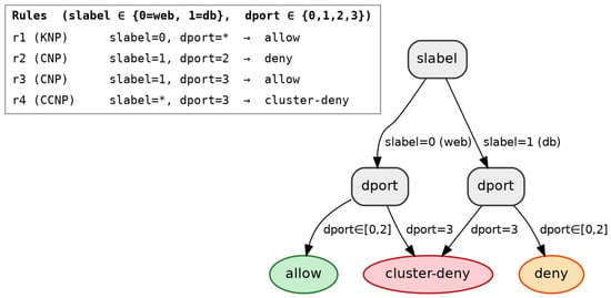
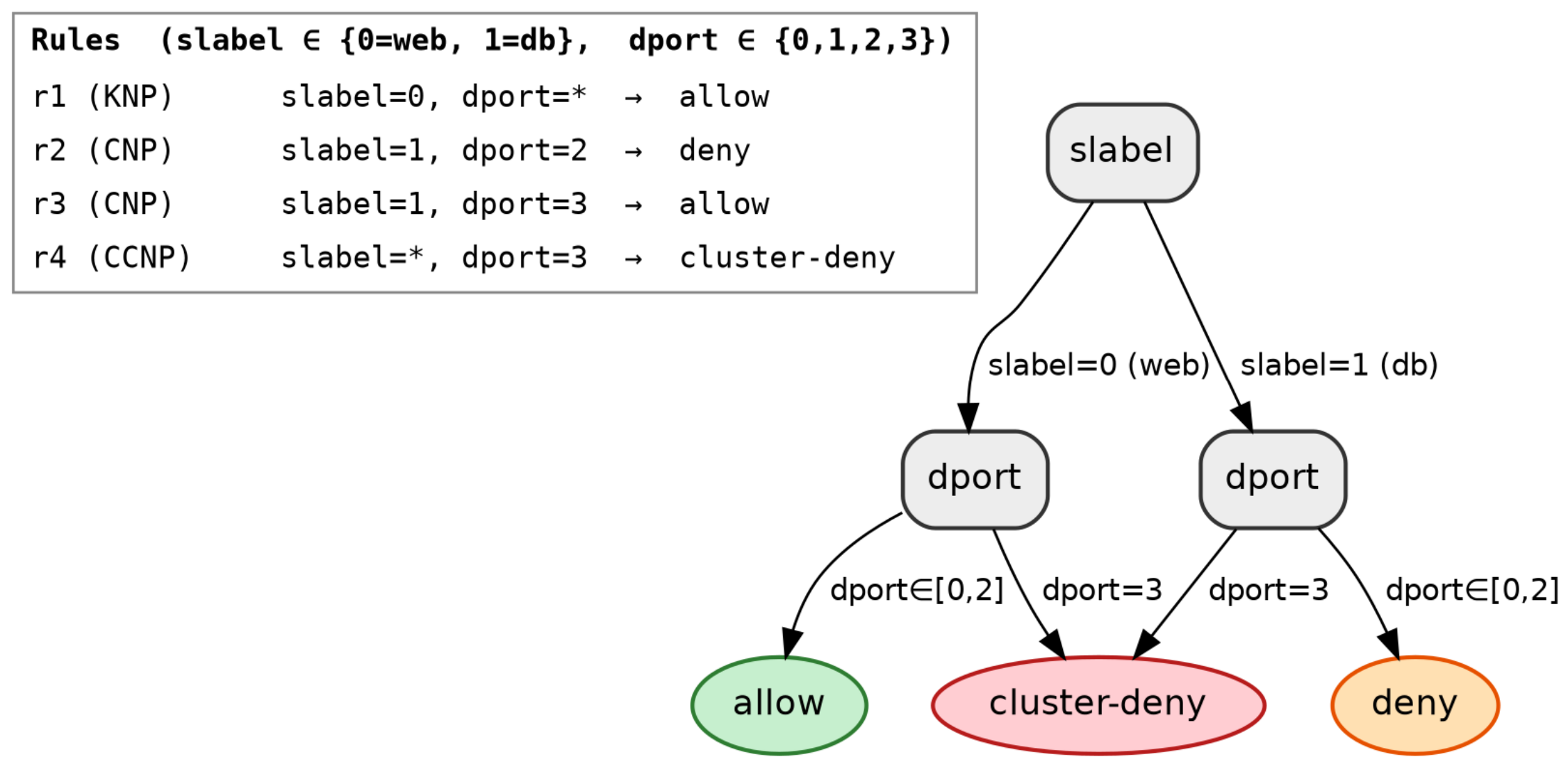
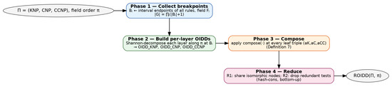
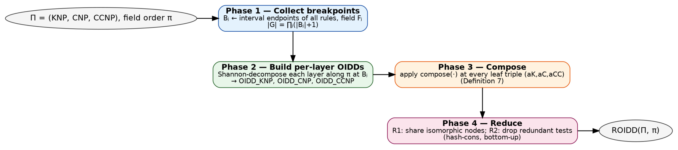
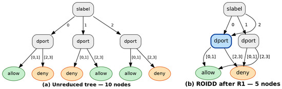
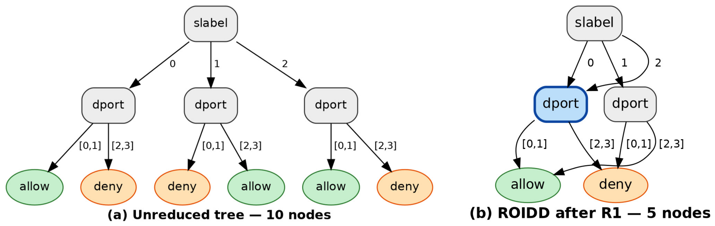
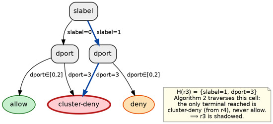
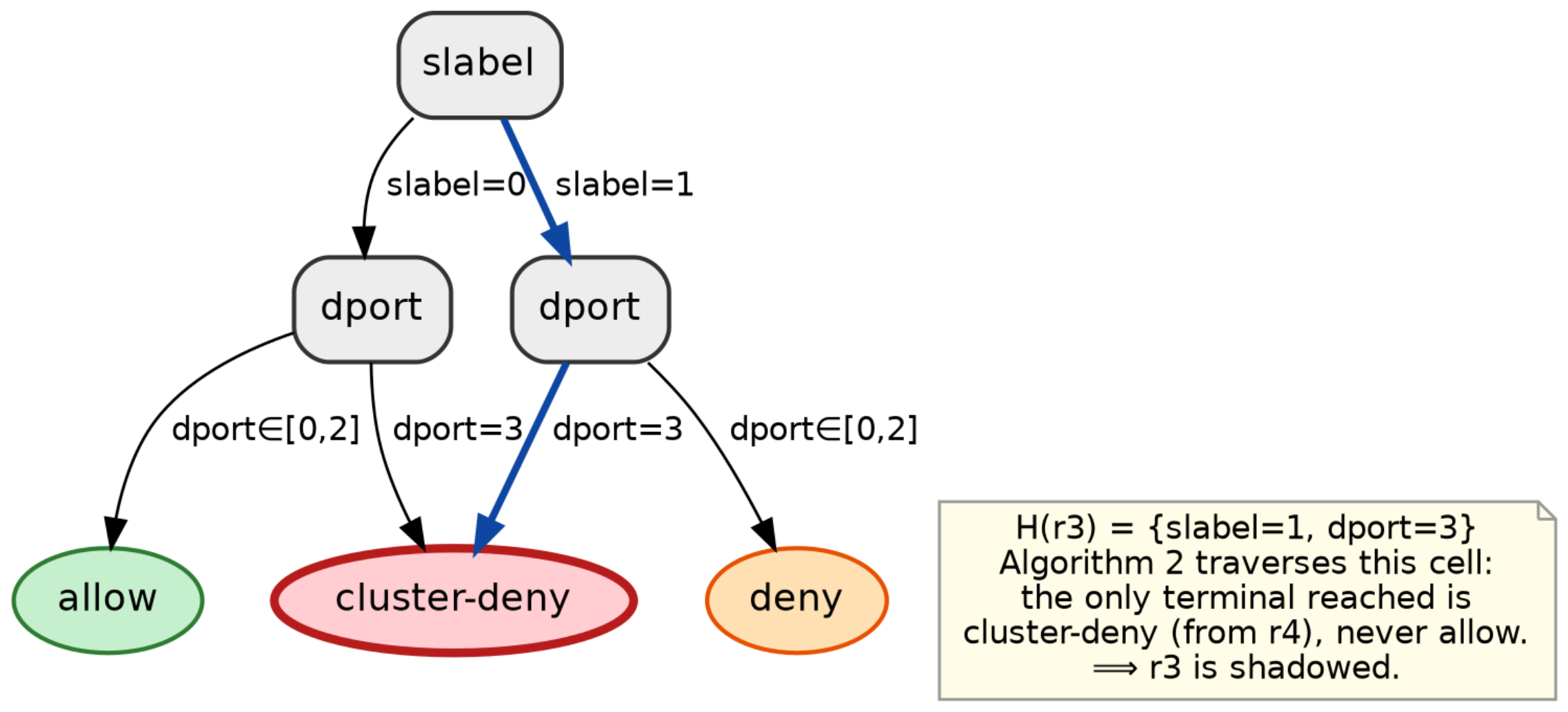

Disclaimer/Publisher’s Note: The statements, opinions and data contained in all publications are solely those of the individual author(s) and contributor(s) and not of MDPI and/or the editor(s). MDPI and/or the editor(s) disclaim responsibility for any injury to people or property resulting from any ideas, methods, instructions or products referred to in the content. |
© 2026 by the authors. Licensee MDPI, Basel, Switzerland. This article is an open access article distributed under the terms and conditions of the Creative Commons Attribution (CC BY) license.