


Abstract
Liquefaction susceptibility mapping supports regional screening where detailed geotechnical data are limited. This study compared two GIS-based weighting approaches for Chiang Rai Province, Thailand: an equal-weight Simple Additive Weighting (SAW) model and an Analytic Hierarchy Process (AHP) model with differential weights. Both used the same four spatial factors-surface geology, slope, distance to rivers, and distance to active faults-with identical scoring criteria and spatial resolution. Internal discrimination was evaluated using 51 documented liquefaction occurrences from the 2014 Mw 6.1 Chiang Rai earthquake and 51 comparison points. SAW and AHP achieved AUC values of 0.923 (95% CI: 0.869–0.976) and 0.933 (95% CI: 0.883–0.983), respectively, with no significant difference (DeLong p = 0.244). The classified maps agreed over 69.86% of the study area, while high and very high susceptibility zones covered 27.56% for SAW and 33.87% for AHP. Pseudo-absence and spatial holdout analyses supported generally robust within-event discrimination. After removing distance to active faults, AHP significantly outperformed SAW (p = 0.022). Because all occurrence data came from one earthquake, results represent event-specific internal evaluation. Overall, SAW provides a transparent baseline, whereas AHP remains useful when differential factor importance is independently justified.
1. Introduction
Soil liquefaction is a phenomenon where saturated, cohesionless soil loses its shear strength and behaves like a liquid during strong earthquake shaking. The process begins when seismic loading causes rapid pore water pressure buildup, reducing effective stress to nearly zero [1,2,3,4]. The resulting ground failure can cause buildings and infrastructure to lose their foundation support, making liquefaction a significant secondary earthquake hazard [5].
Although liquefaction occurs only where conditions are suitable, its consequences can be severe and widespread. The 1964 Alaska and Niigata earthquakes provided landmark demonstrations of the destructive consequences of liquefaction [6,7]. Subsequently, the 1989 Loma Prieta earthquake demonstrated severe liquefaction-related damage in the Marina District of San Francisco, particularly in artificial-fill areas [8]. The 1995 Kobe earthquake revealed major impacts on lifeline and waterfront infrastructure in reclaimed areas [9], consistent with earlier case histories documenting severe liquefaction-induced ground deformation in Niigata [10]. The 2011 Christchurch earthquake further demonstrated city-wide consequences, with sand ejection flooding streets, water and sewage systems severely damaged, and entire neighborhoods demolished [11]. These events confirm that liquefaction can occur in both large and moderate earthquakes given suitable site conditions [12], and that much of this damage is preventable through advance identification of susceptible areas via liquefaction susceptibility mapping [13,14].
Liquefaction susceptibility mapping can be divided into three levels based on data requirements [15]. Level 1 uses existing documents such as earthquake history and geological maps. Level 2 adds aerial photographs and preliminary field surveys. Level 3 relies on in situ testing data such as the Standard Penetration Test (SPT) or Cone Penetration Test (CPT) to calculate liquefaction potential indices [16,17]. While Level 3 provides the highest accuracy for site-specific design, it requires extensive geotechnical data, numerous tests, and substantial costs, making it impractical for regional-scale assessment [18,19]. This limitation is particularly acute in developing countries and remote areas that lack borehole data [20,21,22,23,24]. A practical alternative is to begin with Level 1 screening maps, which can then guide more detailed Level 2 and Level 3 investigations where needed.
For Level 1 mapping, the use of secondary data in Geographic Information Systems (GIS) has gained increasing attention [18,20,25,26]. This approach analyzes existing and easily accessible spatial factors such as geological characteristics, elevation, and distance from water sources as spatial indicators of liquefaction susceptibility [27]. A key step in this process is assigning weights to each factor based on their relative importance. The Analytic Hierarchy Process (AHP) is a commonly used method that determines weights based on systematic pairwise comparisons among factors conducted by experts [28]. Simple Additive Weighting (SAW), in contrast, provides a transparent framework for combining standardized factors and can be implemented using equal weights when differential weighting is not empirically justified. This approach offers transparency and reproducibility, making it potentially suitable for areas where expert knowledge is limited or unavailable [27].
Although GIS-based multi-criteria approaches have been increasingly applied to regional liquefaction susceptibility mapping, two issues remain particularly relevant for data-scarce applications. First, many regional studies have limited empirical evaluation against documented liquefaction occurrences, making it difficult to assess how well susceptibility patterns correspond to observed field evidence [29]. Second, limited evidence is available on whether more complex differential weighting schemes, such as those derived using AHP, provide a measurable improvement over simpler equal-weight approaches when the conditioning factors, scoring criteria, spatial resolution, and evaluation dataset are held constant. A controlled comparison under these conditions is therefore needed to examine the influence of weighting strategy while maintaining the same underlying spatial information.
To address these issues, this study develops and compares two GIS-based liquefaction susceptibility models for Chiang Rai Province: a Simple Additive Weighting (SAW) model implemented using equal weights and an Analytic Hierarchy Process (AHP) model using AHP-derived differential weights. Both models employ the same four spatial factors and scoring criteria and are assessed using the same liquefaction inventory from the 2014 Mw 6.1 Chiang Rai earthquake. The selected factors comprise three site-condition indicators—surface geology, slope, and distance to rivers—and distance to active faults, which is used as a regional proxy for earthquake-triggering intensity. Chiang Rai Province was selected because of its contrasting lowland and mountainous terrain and the availability of documented liquefaction occurrences from this event [30]. By holding the input factors, scoring framework, spatial resolution, and evaluation dataset constant, the study examines how the weighting strategy influences model discrimination and the resulting susceptibility patterns within the present dataset and study framework. The results are intended to provide case-specific evidence on the relative behavior of equal and differential weighting strategies for preliminary regional liquefaction screening in data-scarce settings.
2. Materials and Methods
2.1. Framework and Workflow
This study employs Spatial Multi-Criteria Decision Analysis (SMCDA) within a Geographic Information System (GIS) framework to develop and compare two liquefaction susceptibility models for Chiang Rai Province. The first model applies Simple Additive Weighting (SAW) implemented using equal weights for all factors, while the second applies the Analytic Hierarchy Process (AHP) using differential weights derived from pairwise comparison. To isolate the effect of weighting strategy, both models use identical conditioning factors, scoring criteria, spatial resolution, and evaluation data. The central research question is how the weighting strategy influences model discrimination and the resulting susceptibility patterns within the present dataset and study framework.
The research workflow consists of four phases (Figure 1). The first phase is data preparation. This begins with selecting spatial factors that influence liquefaction through a review of relevant literature, considering both theoretical evidence and data availability in the study area. Four factors were selected: geological characteristics, slope, distance to rivers, and distance to active faults. The first three primarily represent site-condition characteristics, whereas distance to active faults is used as a regional proxy for earthquake-triggering intensity. Spatial data layers for each factor were compiled from geological maps, digital elevation models, and government databases, then processed to a consistent coordinate system and resolution. Each factor was classified into susceptibility classes and assigned scores (1 to 3) based on established scientific criteria, as detailed in Section 2.2. These scoring criteria were defined a priori from the literature and were not calibrated using the liquefaction occurrence inventory. Frequency Ratio (FR) analysis was subsequently applied as a descriptive association check to examine whether the predefined factor classes were consistent with the observed liquefaction pattern from the 2014 Chiang Rai earthquake; no scoring thresholds or susceptibility scores were modified based on the FR results, as described in Section 2.3. Potential dependence among the input factors was also examined using Spearman correlation and Variance Inflation Factor (VIF) analysis.
Figure 1.
Research Workflow for Liquefaction Susceptibility Assessment.
The second phase is model development. Both models use the same set of factors and scoring criteria but differ in how weights are assigned. In this study, the SAW model is implemented using equal weights (0.25) for all four factors, producing a Liquefaction Susceptibility Index (LSI) as the arithmetic mean of the factor scores. The calculation procedure is detailed in Section 2.4.1. The AHP model assigns differential weights based on pairwise comparison, with weights calculated using the eigenvalue method and consistency verified through the Consistency Ratio (CR < 0.1). The pairwise comparison matrix was developed through a consensus-based judgment among the authors, informed by the literature and professional judgment. The calculation procedure is detailed in Section 2.4.2. Both models produce continuous LSI values, which are then classified into four susceptibility levels (low, moderate, high, and very high) using predefined class intervals for map visualization.
The third phase is model evaluation and robustness assessment. First, sensitivity analysis was conducted specifically for the SAW model to examine whether the equal-weighting assumption is robust. Since equal weighting was adopted as the baseline configuration without empirical prioritization of individual factors, it is necessary to examine whether the results change substantially when this assumption is relaxed. Five weight configurations were tested, including the base case (equal weights at 0.25 each) and four cases where each factor is emphasized in turn (55% weight, with the remaining three factors at 15% each). If AUC remains stable across configurations, it indicates that the equal-weighting assumption is defensible and the model is not highly sensitive to weight perturbations. The method is detailed in Section 2.5.1. Second, internal model discrimination was assessed by comparing model outputs against 51 recorded liquefaction occurrence points and 51 comparison points sampled from areas with no recorded liquefaction using Receiver Operating Characteristic (ROC) curve analysis and the Area Under the Curve (AUC) metric. Because the same liquefaction inventory was previously used in the FR analysis, the resulting AUC values are interpreted as internal discrimination estimates rather than independent predictive validation. Optimal classification thresholds for reporting sensitivity and specificity were determined using Youden’s J index [31]. The method is detailed in Section 2.5.2. Third, a DeLong test [32] was applied to determine whether the difference in AUC between the SAW and AHP models is statistically significant, as detailed in Section 2.5.3. Additional robustness analyses included repeated evaluation using five independently generated pseudo-absence sets and a spatially blocked holdout assessment.
The final phase examines the robustness and spatial implications of the model comparison. The influence of the distance-to-active-fault factor was quantified by rerunning both SAW and AHP models without this factor and comparing their AUC, sensitivity, specificity, DeLong results, and mapped susceptibility areas. Spatial agreement and disagreement between the SAW and AHP classifications were also evaluated using a class-difference map. Together, these analyses provide a controlled assessment of how weighting strategy and predictor composition influence model discrimination and spatial susceptibility patterns within the present dataset and study framework.
2.2. Criteria and Scoring Rules
This study selected four key factors for the model: surface geology (Geo-Score), slope (Slope-Score), distance from rivers (River-Score), and distance from active faults (Fault-Score). The first three factors primarily represent site-condition characteristics related to intrinsic liquefaction susceptibility, whereas distance from active faults is included as a regional proxy for earthquake-triggering intensity. These factors were selected for two reasons. First, they represent spatial conditions relevant to liquefaction susceptibility and triggering based on evidence from previous research [14,18,33,34]. Second, data for these factors are available from basic national databases, allowing the model to be practically applied in various areas without requiring data that is difficult or expensive to obtain.
After selecting the factors, the next step is to convert raw data with different units into standardized susceptibility scores. Each factor receives a score from 1 (low susceptibility) to 3 (high susceptibility). This standardization is necessary for two reasons. First, it enables all factors to be combined using the SAW and AHP methods on a common scale. Second, because the primary SAW-AHP comparison uses the same standardized input layers, differences between the two model outputs can be examined with respect to the weighting strategy rather than differences in source data.
2.2.1. Geological Factor (Geo-Score)
The type and age of surface geology strongly influence liquefaction susceptibility. Young, saturated, and unconsolidated sediments, particularly Quaternary deposits of Holocene and Pleistocene age, have significantly higher liquefaction potential than consolidated bedrock or pre-Quaternary materials [2,34]. This relationship is well established in soil mechanics: Youd et al. [4] reported that coarse-grained soils from the late Quaternary period are the most susceptible, while pre-Quaternary sediments have very low susceptibility, a finding consistent with the principle that sediment age directly affects soil density and resistance to seismic loading [33,35,36]. Regional-scale liquefaction susceptibility studies further confirm that geological age is among the most influential spatial factors [5,18,26].
The scoring criteria in this study classify geological map units into two groups based on whether the surface deposit is of Quaternary age. Quaternary sediments, including unconsolidated Pleistocene and Holocene deposits, receive a Geo-Score of 3 (high susceptibility), while non-Quaternary units such as consolidated bedrock receive a score of 1 (low susceptibility). No intermediate score is assigned because the geological data available in the study area classify units at the general Quaternary level without subdivision into finer age categories. This binary classification is consistent with the resolution of basic geological maps typically available in developing countries such as Thailand, making the criteria applicable to existing databases without requiring high-resolution geological mapping.
2.2.2. Slope Factor (Slope-Score)
Slope is commonly used as a spatial indicator of liquefaction susceptibility because it reflects the geomorphological setting of an area. Flat to gently sloping terrain such as floodplains, coastal plains, and valley floors typically contain thick accumulations of loose, saturated Quaternary sediments with shallow groundwater tables, which are conditions favorable for liquefaction. Furthermore, field observations from the 2014 Chiang Rai earthquake revealed that some liquefaction occurrences were located far from major rivers but near man-made water features such as excavated ponds that do not appear in available hydrological maps. In such cases, slope serves as a complementary indicator of shallow groundwater conditions that the distance-to-river factor alone cannot capture. In contrast, steep terrain is generally associated with bedrock or well-consolidated materials where liquefiable sediments rarely accumulate. Empirical evidence confirms that liquefaction predominantly occurs in flat to gently sloping areas [2,4,33,34,36,37,38].
Based on this evidence, the Slope-Score was derived from percent slope calculated from a digital elevation model and classified into three levels as shown in Table 1. Areas with 0–5% slope receive a score of 3 (high susceptibility), areas with >5–15% receive a score of 2 (moderate susceptibility), and areas with >15% receive a score of 1 (low susceptibility). These ranges are consistent with terrain classification standards from USDA [39] and FAO [40].
Table 1.
Scoring criteria for the Slope Factor (Slope-Score).
2.2.3. Hydrological Factor (River-Score)
A high groundwater table is a fundamental condition for liquefaction because soil needs to be saturated or nearly saturated for pore water pressure to build up during shaking [2,34]. However, direct groundwater level data are often limited or vary spatially and temporally. In regional-scale assessment, distance from surface water sources such as rivers is therefore commonly used as a proxy for shallow groundwater conditions [5,18]. This proxy is supported by empirical evidence showing that areas near rivers tend to have shallow groundwater, young water-deposited sediments, and conditions favorable for liquefaction [4,34].
Based on this evidence, the River-Score was defined according to horizontal distance from each location to the nearest major surface water source, classified into three levels as shown in Table 2. Areas within 0–100 m receive a score of 3 (high susceptibility), areas at distances >100–1000 m receive a score of 2 (moderate susceptibility), and areas beyond 1000 m receive a score of 1 (low susceptibility).
Table 2.
Scoring criteria for the Hydrological Factor (River-Score).
2.2.4. Earthquake Source Factor (Fault-Score)
Strong ground shaking is the trigger for liquefaction. Without sufficient seismic energy, even highly susceptible soils will not liquefy [43]. In detailed site-specific analysis, shaking intensity is typically represented by parameters such as Peak Ground Acceleration (PGA) or Peak Ground Velocity (PGV) [16,17,44]. However, incorporating these parameters into regional-scale models requires full earthquake scenario modeling, which may not be feasible for preliminary screening. Moreover, in Thailand, the national seismic design standard (DPT 1311-61) assigns a uniform PGA value to the entire Chiang Rai Province, thereby providing no spatial variation within the study area for susceptibility differentiation. Distance from active faults is therefore used as a proxy for relative shaking intensity, based on the principle that ground motion attenuates with increasing distance from the seismic source.
Accordingly, distance from active faults is treated differently from the three site-condition factors. It does not represent an intrinsic soil property but rather serves as a simplified trigger-related spatial proxy for regional screening. Because its spatial relationship with the 2014 Chiang Rai earthquake may influence model discrimination, its contribution is further examined through a separate no-fault ablation analysis. The scoring criteria for distance to active faults are summarized in Table 3.
Table 3.
Scoring criteria for the Earthquake Source Factor (Fault-Score).
The scoring criteria for all four factors are summarized in Table 4. All spatial data layers were prepared in raster format with a uniform spatial resolution of 30 m and reclassified according to the scoring criteria summarized in Table 4. The resulting standardized factor maps are presented in Figure 2, including (a) Geo-Score, (b) Slope-Score, (c) River-Score, and (d) Fault-Score. Each raster cell was assigned a susceptibility score ranging from 1 (low susceptibility) to 3 (high susceptibility) according to the predefined criteria. These criteria were established a priori from the literature and were not adjusted using the liquefaction occurrence inventory. These standardized factor maps were subsequently used as the direct spatial inputs for both the SAW and AHP models.
Table 4.
Summary of standardized susceptibility scoring criteria.
Figure 2.
Standardized input factor maps: (a) Geo-Score, (b) Slope-Score, (c) River-Score, and (d) Fault-Score.
2.3. Statistical Analysis of Spatial Relationships
Two complementary statistical analyses were conducted to examine the relationships between the selected spatial factors and the observed liquefaction inventory and to assess potential dependence among the input factors. Frequency Ratio (FR) analysis was used as a descriptive association check, while Spearman rank correlation and Variance Inflation Factor (VIF) analyses were used to evaluate factor correlation and multicollinearity.
2.3.1. Frequency Ratio (FR) Association Analysis
The scoring criteria described in Section 2.2 were defined a priori based on the literature and were not calibrated using the 51 liquefaction occurrence points. To examine whether these predefined factor classes were spatially consistent with the observed liquefaction pattern in the study area, this study applied the Frequency Ratio (FR) method to examine the spatial relationship between recorded liquefaction locations and each factor subclass. FR is a bivariate probability model widely used for natural hazard susceptibility assessment [48,49,50]. The method compares the proportion of liquefaction occurrences in each factor subclass with the area proportion of that subclass. For example, if Quaternary sediments cover 30% of the study area but contain 60% of all liquefaction occurrences, this indicates a strong positive spatial association.
The Frequency Ratio is calculated as:
where
Nclass = Number of liquefaction occurrence points in each subclass;
Ntotal = Total number of liquefaction occurrence points in the study area (=51);
Aclass = Area of each subclass (km2);
Atotal = Total area of the study area (km2).
An FR value greater than 1 indicates a higher-than-average liquefaction occurrence density within a factor subclass, while an FR value less than 1 indicates a lower-than-average occurrence density [48,49]. In this study, the FR results were examined to determine whether subclasses assigned higher susceptibility scores generally exhibited higher liquefaction occurrence densities and whether subclasses assigned lower scores exhibited lower occurrence densities. No class boundaries, susceptibility scores, or factor weights were modified based on the FR results. Accordingly, FR is interpreted as a descriptive association check of the predefined literature-based scoring criteria rather than as an independent validation procedure.
2.3.2. Correlation and Multicollinearity Assessment
To assess whether the four spatial factors contained strongly overlapping information, Spearman rank correlation and Variance Inflation Factor (VIF) analyses were conducted. A total of 5000 spatially distributed random sampling points were generated within the common valid area of the four input factors, using a minimum spacing of 30 m and a fixed random seed of 20260929. After excluding locations with incomplete factor values, 4984 samples were retained for analysis.
Spearman rank correlation was used to examine the direction and strength of pairwise associations among the raw predictor values for surface geology, slope, distance to rivers, and distance to active faults, rather than the reclassified susceptibility scores. VIF was subsequently calculated for each factor to assess potential multicollinearity when the four factors were considered simultaneously. These analyses were used to evaluate whether substantial redundancy among the input factors could influence the interpretation of the SAW and AHP model comparison.
2.4. Spatial Multi-Criteria Decision Analysis Modeling
After converting all four factors into standardized susceptibility scores (Section 2.2) and examining their spatial associations with the recorded liquefaction occurrences through the descriptive FR analysis in Section 2.3, the next step is to combine these factors into a single Liquefaction Susceptibility Index (LSI) for every pixel in the study area. This integration uses Spatial Multi-Criteria Decision Analysis (SMCDA) within GIS, where each factor is assigned a weight reflecting its relative importance and the weighted scores are summed.
This study compares two weighting strategies within the same additive GIS framework. In the first, the Simple Additive Weighting (SAW) model is implemented using equal weights for all four factors, providing a transparent baseline without differential prioritization among factors. In the second, differential weights are derived using the Analytic Hierarchy Process (AHP) through pairwise comparison and consistency checking. Because both models use identical spatial factors, scoring criteria, spatial resolution, and evaluation data, the primary comparison provides a controlled assessment of how the weighting strategy influences model discrimination and the resulting susceptibility patterns within the present dataset and study framework.
2.4.1. Model 1: Simple Additive Weighting (SAW)
In this study, the SAW model was implemented using equal weights for all four factors. Equal weighting was adopted as a transparent baseline because there was insufficient empirical evidence from the study area to justify differential prioritization of individual factors and to minimize potential bias from subjective weighting judgments [51,52]. The Liquefaction Susceptibility Index is calculated as:
where wi = 0.25 for each factor and Scorei is the standardized susceptibility score (1–3) of each factor from Section 2.2. The LSISAW values range from 1.0, representing the lowest susceptibility, to 3.0, representing the highest susceptibility. The index was calculated for each raster cell using GIS map algebra. This weighted linear combination approach has been applied in previous spatial susceptibility studies [51,53,54].
LSISAW = (0.25 × Geo-Score) + (0.25 × Slope-Score) + (0.25 × River-Score) + (0.25 × Fault-Score)
2.4.2. Model 2: Analytic Hierarchy Process (AHP)
The AHP model determines factor weights through systematic pairwise comparison, allowing each factor to receive a weight reflecting its assessed importance relative to the others [28]. This method has been widely applied in disaster risk assessment [5,51,55].
Pairwise judgments were assigned using Saaty’s [28] scale, in which larger values indicate greater relative importance of one factor over another and reciprocal values are assigned to the reverse comparison. In this study, the pairwise comparison matrix was developed through a consensus-based judgment process among the authors. The authors jointly reviewed the relevant literature and discussed the relative roles of the four factors until a single comparison matrix was agreed upon. Therefore, separate expert matrices were not elicited or mathematically aggregated. The literature was used to support the scientific rationale for the relative judgments rather than to prescribe the exact numerical Saaty values. The six unique pairwise comparisons, their assigned Saaty values, rationales, and supporting references are summarized in Table 5.
Table 5.
Rationale for the AHP pairwise comparisons.
The pairwise comparisons are arranged in a 4 × 4 matrix containing six unique comparison pairs. Weights are then derived by calculating the principal eigenvector of the matrix, producing normalized weights that sum to 1.0 [28]. To verify logical consistency, the Consistency Ratio (CR) is calculated. A CR value below 0.10 is considered acceptable [5,28,56]. The resulting weights and consistency statistics are reported in Section 4.2.2.
Once the weights pass the consistency check, the AHP-based Liquefaction Susceptibility Index is calculated as:
where W1, W2, W3, and W4 are the weights derived from the AHP. Unlike the SAW model, which assigns equal weights to all factors, the AHP weights differ for each factor according to its assessed importance. The LSIAHP values range from 1.0 (lowest susceptibility) to 3.0 (highest susceptibility). The AHP-based LSI was calculated using the same GIS map-algebra procedure as the SAW model.
LSIAHP = (W1 × Geo-Score) + (W2 × Slope-Score) + (W3 × River-Score) + (W4 × Fault-Score)
2.5. Model Evaluation and Robustness Assessment
To evaluate model discrimination and assess the robustness of the results, six complementary analyses were conducted: (1) sensitivity analysis of the SAW assumption, (2) internal discrimination assessment using ROC-AUC, (3) statistical comparison of correlated AUCs using the DeLong test, (4) sensitivity analysis using multiple independently generated pseudo-absence sets, (5) a spatially blocked robustness assessment, and (6) a no-fault ablation analysis to quantify the influence of distance to active faults.
2.5.1. Sensitivity Analysis of the SAW Model
The SAW model uses equal weights for all four factors as the base case, with each factor assigned a weight of 0.25. To evaluate whether model discrimination is sensitive to this equal-weighting assumption, a one-at-a-time sensitivity analysis was conducted, following an approach commonly applied in natural hazard studies [23,51].
Five weight configurations were evaluated. The base case assigns an equal weight of 0.25 to each factor. In Cases 1–4, the weight of one factor was increased to 0.55, while the weights of the remaining three factors were reduced to 0.15 each, maintaining a total weight of 1.0. Specifically, Case 1 emphasizes geology, Case 2 emphasizes slope, Case 3 emphasizes distance to rivers, and Case 4 emphasizes distance to active faults.
The AUC obtained from each sensitivity case was compared with that of the equal-weight base case to assess the stability of model performance under substantial changes in factor weights. The sensitivity cases were designed solely to evaluate the robustness of the equal-weighting assumption and were not intended to identify or optimize an alternative set of factor weights. Accordingly, the sensitivity configurations were not used to recalibrate the SAW model based on the highest observed AUC. This analysis therefore evaluates sensitivity to weight perturbation rather than optimizing the model against the available evaluation dataset.
2.5.2. Internal Discrimination Assessment Using ROC-AUC
Model discrimination was assessed using Receiver Operating Characteristic (ROC) curve analysis and the Area Under the Curve (AUC), which are standard tools for evaluating natural hazard models [49,50]. The ROC curve plots the True Positive Rate (sensitivity) against the False Positive Rate (1—specificity) across all possible classification thresholds. The AUC value ranges from 0.5 (no discrimination) to 1.0 (perfect discrimination).
The primary evaluation dataset consists of 51 recorded liquefaction occurrence points from the 2014 Chiang Rai earthquake as positive samples and 51 comparison points sampled from areas with no recorded liquefaction. Because the absence of a recorded liquefaction feature does not necessarily represent a confirmed true absence, these comparison locations are not interpreted as field-verified non-liquefaction sites.
The same 51 liquefaction occurrence points were previously used in the FR descriptive association analysis. However, the factor classes and scoring criteria had been defined a priori from the literature and were not modified based on the FR results. Nevertheless, because the occurrence inventory is reused in the ROC analysis, the resulting AUC values are interpreted as internal discrimination estimates rather than as independent predictive validation.
Optimal classification thresholds for reporting sensitivity and specificity were determined using Youden’s J index, which maximizes the sum of sensitivity and specificity [31]. Because these thresholds were selected and evaluated using the same 102-point dataset, the corresponding sensitivity and specificity values are interpreted as apparent or internal performance measures.
ROC-AUC analysis was applied at two levels: individual-factor discrimination and comparison of the overall SAW and AHP models. AUC values are reported together with their 95% confidence intervals rather than being primarily interpreted using qualitative performance categories. The standard errors and 95% confidence intervals of the individual AUC estimates were calculated using the approximation method of Hanley and McNeil [57].
2.5.3. Statistical Comparison Using DeLong Test
To determine whether the difference in AUC between the SAW and AHP models is statistically significant, a DeLong test was applied [32]. This non-parametric test compares two correlated ROC curves derived from the same dataset by estimating the variance of the AUC difference using structural components. The test produces a Z-statistic and a corresponding p-value. In addition to the p-value, the paired AUC difference and its 95% confidence interval were reported to quantify the magnitude and uncertainty of the difference between the two models. If p > 0.05, the difference in AUC is considered not statistically significant, indicating that no statistically significant difference in discrimination was detected between the two models.
ROC-AUC values, 95% confidence intervals, and paired DeLong tests were calculated in Microsoft Excel for Microsoft 365 using formula-based implementations.
2.5.4. Pseudo-Absence Sensitivity Analysis
To evaluate whether the model discrimination estimates were sensitive to the selection of comparison locations, five independent pseudo-absence datasets were generated. A 500 m exclusion buffer was applied around the 51 recorded liquefaction occurrence points, and pseudo-absence points were sampled only from the common valid spatial coverage of all model factors. Each replicate contained 51 pseudo-absence points, preserving a 1:1 ratio with the occurrence inventory.
A minimum spacing of 30 m was imposed between sampled points, corresponding to the raster resolution, and fixed random seeds of 5001, 5002, 5003, 5004, and 5005 were used for reproducibility. The pseudo-absence points were not stratified by terrain or geographic subregion. Areas without a complete accessibility or field-inspection record were not separately excluded because a comprehensive reconnaissance-coverage mask was unavailable.
SAW and AHP AUC values were recalculated for each replicate to assess the sensitivity of model discrimination to alternative pseudo-absence selections. The replicate-specific results were summarized using the mean, standard deviation, and range of AUC values; p-values from the individual DeLong tests were not averaged.
2.5.5. Spatially Blocked Robustness Assessment
An additional post hoc spatially blocked assessment was conducted to examine whether model discrimination remained stable when evaluated in a geographically separated portion of the 2014 liquefaction inventory. The southern portion of the inventory, defined using the first quartile of the northing coordinates (northing ≤ 2,172,170.56 m), was used as the holdout block. This block contained 13 liquefaction occurrence points and 11 pseudo-absence points from the first pseudo-absence replicate.
ROC-AUC, sensitivity, specificity, and accuracy were calculated for both models within this spatial holdout. Because all occurrence points originate from the same 2014 earthquake event, this analysis is interpreted as a spatial robustness assessment rather than as independent event-based validation.
2.5.6. No-Fault Ablation Analysis
To quantify the influence of the distance-to-active-fault factor on the model results, an ablation analysis was conducted by removing Fault-Score from both the SAW and AHP models. For the SAW model, equal weighting was maintained among the three remaining factors (surface geology, slope, and distance to rivers), with each assigned a weight of 1/3. For the AHP model, the original pairwise judgments among the three remaining factors were retained, and the factor weights were recalculated from the reduced 3 × 3 comparison matrix using the principal eigenvector method. The weights were recomputed rather than obtained by simply renormalizing the original four-factor weights, and the consistency of the reduced matrix was assessed using the same CR < 0.10 criterion applied to the full AHP model.
The full and no-fault models were evaluated using the same internal evaluation dataset. Their performance was compared using AUC with 95% confidence intervals, sensitivity, specificity, accuracy, and paired DeLong tests. Changes in the spatial distribution of susceptibility classes were also assessed by comparing the mapped area proportions of the full and no-fault models. The same class-break thresholds used for the corresponding full models were retained for the no-fault maps to isolate the effect of removing the fault-distance factor.
3. Study Area
This study selected Chiang Rai Province as the study area because of the recorded evidence of liquefaction from the Mw 6.1 earthquake on 5 May 2014 [30], which provides a documented liquefaction occurrence inventory for empirical evaluation of the developed susceptibility maps. The province also has geological and tectonic characteristics favorable for liquefaction, including loose alluvial deposits in river floodplains and several active faults crossing the area.
3.1. Topography
Chiang Rai Province is located in the northernmost highland area of Thailand, covering approximately 11,678 km2. The province borders Myanmar and Lao PDR to the north, and Chiang Mai, Lampang, and Phayao provinces to the west and south.
The topography is diverse, with approximately 65% consisting of mountains and high ranges oriented in a nearly north–south direction, with elevations of 500–2000 m above mean sea level. The remaining approximately 35% is lowland distributed in intermontane basins and river floodplains, which are areas with dense settlement and economic activities. The province is drained by two main river systems: the Kok River, flowing through central Chiang Rai city, and the Ing River in the eastern part, both of which ultimately discharge into the Mekong River. These river systems transport and deposit sediments from the highland areas into the lowland basins, resulting in thick accumulations of alluvial deposits in the floodplains—a key condition for liquefaction susceptibility in the study area [58,59], as shown in Figure 3.
Figure 3.
Topographic map and major river systems of Chiang Rai Province.
3.2. Geological Setting
The geology of Chiang Rai Province is diverse, resulting from tectonic processes in the Southeast Asian region spanning over 345 million years [58,59]. The overall geological structure can be divided into two main parts: bedrock forming the surrounding mountains, and Quaternary sediments accumulated in the central basins.
The bedrock in mountainous areas consists of Paleozoic and Mesozoic sedimentary rocks (shale, sandstone, limestone), low-grade metamorphic rocks (phyllite, slate, schist), and igneous rocks (granite, basalt). These materials are well-consolidated with high strength and are not susceptible to liquefaction.
In contrast, the lowland basins contain Quaternary deposits (2.6 Ma to present) that are directly relevant to liquefaction. These loose, unconsolidated sediments can be classified into three types based on depositional environment. The first type is floodplain deposits, consisting of clay, sandy clay, and fine to coarse sand, found in the Kok River and Ing River floodplains. These deposits typically have shallow groundwater and are therefore generally associated with higher liquefaction susceptibility. The second type is terrace deposits, consisting of gravel, sand, and laterite, found at elevations above flood level with typically deeper groundwater and lower susceptibility. The third type is alluvial fan deposits, formed at mountain bases by streams flowing from steep valleys, often poorly sorted with diverse grain sizes.
3.3. Seismotectonic Setting
Chiang Rai Province is located near several active fault systems in northern Thailand, as shown in Figure 4. These fault systems result from stress accumulation caused by the ongoing collision of the Indian Plate with the Eurasian Plate.
Figure 4.
Active fault systems in Chiang Rai Province.
The major faults affecting the province include the Mae Chan Fault, a left-lateral strike-slip fault approximately 118 km long oriented in a southwest-northeast direction; the Mae Ing Fault to the east; the Mae Tha Fault to the south; and the Phayao Fault Zone, which consists of the Mae Lao Fault (northeast-southwest orientation) and the Phayao Fault (north–south orientation). These two faults intersect at the boundary between Chiang Rai and Phayao provinces. The presence of multiple active faults crossing the area makes Chiang Rai Province one of the most seismically active regions in Thailand.
The Mw 6.1 earthquake on 5 May 2014 is considered the largest earthquake in modern Thai history [30]. The epicenter was located at the junction of the Mae Lao Fault and the Phayao Fault, indicating a conjugate fault system mechanism. With a focal depth of approximately 7 km, the shallow rupture produced intense ground shaking at the surface. The earthquake caused widespread damage, with over 8000 buildings damaged, 1 fatality, and over 100 injuries, along with secondary hazards including landslides and liquefaction near the epicenter [60,61], as shown in Figure 5. The 51 documented liquefaction points from this event constitute the occurrence inventory used for the internal model evaluation in this study.
Figure 5.
Sand boils observed following the 2014 Chiang Rai earthquake.
4. Results
The results are presented in five parts: factor association and predictor dependence, susceptibility mapping, sensitivity analysis, internal model evaluation and robustness assessment, and no-fault ablation analysis.
4.1. Factor Association and Predictor Dependence
4.1.1. Frequency Ratio Association Analysis
The Frequency Ratio results for all four factors are presented in Table 6. Across all factors, subclasses assigned high susceptibility scores (Rating = 3) consistently show FR values greater than 1, while subclasses assigned low scores (Rating = 1) show FR values less than 1, indicating that the predefined scoring criteria are generally consistent with the observed spatial distribution of liquefaction occurrences. As described in Section 2.3.1, these criteria were defined a priori and were not modified based on the FR results; therefore, the FR analysis is interpreted as a descriptive association check rather than as an independent validation procedure.
Table 6.
Frequency Ratio analysis results for liquefaction controlling factors.
The distance-to-river factor shows the strongest spatial association: areas within 0–100 m have an FR of 6.89, meaning they have nearly seven times higher liquefaction occurrence density than average, despite covering only 2.85% of the province. For geology, Quaternary sediments (FR = 2.84) contain 96.08% of all occurrences, while bedrock areas (FR = 0.06) contain only 3.92%. The slope factor shows 62.75% of occurrences in areas with less than 5% slope (FR = 2.45), while areas with slope greater than 15% have an FR of only 0.04. For distance to faults, all 51 occurrences (100%) are located within 10 km of active faults (FR = 1.70), with no occurrences recorded at greater distances. This concentration should be interpreted in the context of the 2014 earthquake event, because the occurrence inventory was generated by a single earthquake associated with the local active-fault system.
4.1.2. Correlation and Multicollinearity Analysis
Spearman rank correlation and Variance Inflation Factor (VIF) analyses were used to examine dependence among the four spatial factors. Of the 5000 randomly sampled locations, 4984 contained complete values for all factors and were included in the analysis. The resulting correlation coefficients and VIF values are summarized in Table 7.
Table 7.
Spearman rank correlations and Variance Inflation Factors for the spatial factors.
The strongest pairwise relationship was observed between geology and slope (ρ = −0.661), followed by slope and distance to rivers (ρ = 0.498) and geology and distance to rivers (ρ = −0.469). Correlations involving distance to active faults were comparatively weak, with coefficients of −0.016 with geology, −0.005 with slope, and 0.278 with distance to rivers.
VIF values ranged from 1.133 to 1.614, with the highest values obtained for slope (1.614) and geology (1.607). All VIF values were well below commonly used thresholds for problematic multicollinearity, indicating that the four factors did not exhibit severe multicollinearity within the sampled study area.
4.2. Liquefaction Susceptibility Mapping from Combined Factors
This section presents the liquefaction susceptibility maps produced by the SAW and AHP models, followed by a spatial comparison of the two outputs.
4.2.1. SAW Model Results
The SAW model calculates the LSI as the arithmetic mean of the four equally weighted factor scores (0.25 each), as described in Section 2.4.1. The resulting susceptibility map was classified into four predefined susceptibility levels: low, LSI ≤ 1.50; moderate, 1.50 < LSI ≤ 2.00; high, 2.00 < LSI ≤ 2.50; and very high, LSI > 2.50, as shown in Figure 6.
Figure 6.
Liquefaction susceptibility map produced by the SAW model.
High and very high susceptibility areas are concentrated in the Kok River and Ing River floodplains, where multiple favorable conditions coincide, including loose Quaternary sediments, low slopes, proximity to rivers, and short distances to active faults. In contrast, surrounding mountainous areas with bedrock and steep slopes are predominantly classified as low susceptibility. The spatial distribution of susceptibility levels is summarized in Table 8. Low susceptibility accounts for 52.89% of the province, while high and very high susceptibility areas together cover 3218.46 km2 (27.56%), mainly corresponding to lowland and river-floodplain areas.
Table 8.
Area distribution of susceptibility levels from the SAW model.
4.2.2. AHP Model Results
The AHP model uses weights derived from pairwise comparison. The pairwise comparison procedure and the rationale for the six consensus judgments are described in Section 2.4.2. The resulting comparison matrix had a Consistency Ratio (CR) of 0.016, below the acceptable threshold of 0.10, indicating acceptable consistency. The derived factor weights are presented in Table 9. Geology received the highest weight (52.22%), followed by distance to river and distance to fault (19.98% each), and slope (7.81%).
Table 9.
Factor weights derived from the AHP model.
The resulting susceptibility map was classified into four predefined susceptibility levels: low, LSI ≤ 1.49985; moderate, 1.49985 < LSI ≤ 1.99980; high, 1.99980 < LSI ≤ 2.49975; and very high, LSI > 2.49975, as shown in Figure 7. The spatial distribution of susceptibility levels is summarized in Table 10. High and very high susceptibility areas together account for 33.87% of the province (3955.34 km2), compared with 27.56% for the SAW model. Low susceptibility covers 59.21% of the province, while the very high susceptibility class accounts for 22.51%.
Figure 7.
Liquefaction susceptibility map produced by the AHP model.
Table 10.
Area distribution of susceptibility levels from the AHP model.
4.2.3. Spatial Comparison of SAW and AHP Models
The AHP model classifies a larger proportion of the province as high and very high susceptibility (33.87%) compared with the SAW model (27.56%), corresponding to a difference of approximately 737 km2. The most pronounced difference occurs in the very high susceptibility class, which covers 22.51% of the study area in the AHP model compared with 7.55% in the SAW model. The area proportions for the two models are summarized in Table 11.
Table 11.
Comparison of area proportions between SAW and AHP models.
Both models identify the main susceptible areas in the Kok and Ing River floodplains. A cell-by-cell comparison showed that 69.86% of the study area was assigned to the same susceptibility class by both models, while 30.14% was classified differently. AHP assigned a higher susceptibility class than SAW over 21.87% of the study area and a lower class over 8.27%. Most disagreements involved one susceptibility level, while differences in two levels accounted for only 0.37% of the study area. The spatial pattern of agreement and disagreement is shown in Figure 8.
Figure 8.
Spatial differences between the SAW and AHP susceptibility maps.
4.3. Sensitivity Analysis
To examine whether the equal-weighting assumption of the SAW model is robust, five weight configurations were tested using the one-at-a-time approach. The base case uses equal weights (0.25 each), while Cases 1–4 increase the weight of one factor to 0.55 with the remaining factors reduced to 0.15, as summarized in Table 12.
Table 12.
Weight configurations for sensitivity analysis.
4.3.1. Spatial Distribution of Sensitivity Cases
The susceptibility maps from the five weight configurations are compared in Figure 9, and the area proportions for each susceptibility level are summarized in Table 13. The same predefined class intervals used for the SAW base case (low, LSI ≤ 1.50; moderate, 1.50 < LSI ≤ 2.00; high, 2.00 < LSI ≤ 2.50; and very high, LSI > 2.50) were applied to all five sensitivity maps in Figure 9. The combined high and very high susceptibility area ranges from 15.37% in Case 3 (distance-to-river emphasis) to 64.76% in Case 4 (distance-to-fault emphasis), compared with 27.56% in the base case. Case 1 (geology emphasis) produces a pattern similar to the AHP model, with expanded susceptible areas in Quaternary sediment zones. Case 4 concentrates susceptibility within approximately 10 km of active faults, resulting in the largest combined high and very high proportion.
Figure 9.
Susceptibility maps under five sensitivity-analysis weight configurations.
Table 13.
Area distribution of susceptibility levels across sensitivity analysis cases.
Despite these differences in area proportions, the main susceptible zones remain concentrated in the lowland and floodplain areas across all configurations, while mountainous areas remain predominantly low susceptibility.
4.3.2. Discrimination Stability Across Weighting Cases
The AUC values for the five weight configurations are presented in Table 14. AUC values ranged from 0.8750 to 0.9429 across the tested configurations. Case 2, which emphasized slope, produced the lowest AUC (0.8750), whereas Case 3, which assigned greater weight to distance to rivers, produced the highest AUC (0.9429), compared with 0.9225 for the equal-weight base case.
Table 14.
AUC values from sensitivity analysis.
The purpose of these alternative configurations was to evaluate the sensitivity of the model to changes in factor weights rather than to identify an optimal weighting scheme. Overall, the relatively limited variation in AUC (mean = 0.9199; SD = 0.0263), despite substantial changes in individual factor weights from 0.15 to 0.55, indicates that discrimination remained comparatively stable across the tested weighting configurations, although the mapped susceptibility proportions varied substantially, as shown in Section 4.3.1.
4.4. Internal Model Evaluation and Robustness Assessment
This section evaluates the internal discrimination and robustness of the SAW and AHP models using the 2014 Chiang Rai liquefaction inventory. Because the same occurrence inventory was also used in the FR analysis, the following results are interpreted as internal evaluation and robustness evidence rather than as independent predictive validation.
4.4.1. Occurrence Coverage Across Susceptibility Classes
The 51 recorded liquefaction occurrence points were overlaid on the susceptibility maps from both models, as shown in Figure 10. The SAW model placed 50 of 51 points (98.04%) within the combined high and very high susceptibility classes, while the AHP model placed 49 points (96.08%) within these classes. No occurrence points were located in the low susceptibility class for either model. The distribution of occurrence points across susceptibility classes is summarized in Table 15.
Figure 10.
Spatial overlay of liquefaction occurrence points on susceptibility maps from the SAW model (left) and AHP model (right).
Table 15.
Distribution of liquefaction occurrence points across susceptibility levels between SAW and AHP models.
These coverage rates differ from the sensitivity values reported in Section 4.4.3 because they are based on the predefined susceptibility classes used for map visualization, whereas sensitivity is calculated from the optimal Youden’s J threshold applied to the continuous LSI values.
4.4.2. Individual-Factor Discrimination
Individual-factor ROC analysis showed differences in discrimination among the four spatial factors. Geology produced an AUC of 0.984 (95% CI: 0.959–1.000), followed by distance to rivers with an AUC of 0.970 (95% CI: 0.936–1.000) and slope with an AUC of 0.887 (95% CI: 0.821–0.953). Distance to active faults produced a nominal AUC of 1.000.
The perfect separation obtained for distance to active faults reflects the spatial configuration of the single-event dataset, in which all 51 recorded liquefaction occurrences were located within 10 km of active faults. Accordingly, this value should be interpreted as event-specific discrimination rather than as evidence of perfect predictive ability for other earthquake scenarios.
4.4.3. Full-Model Internal Discrimination and Statistical Comparison
The SAW and AHP models were evaluated using the primary dataset of 51 liquefaction occurrence points and 51 comparison points. The ROC curves are shown in Figure 11, and the corresponding performance statistics are summarized in Table 16. SAW yielded an AUC of 0.923 (95% CI: 0.869–0.976), while AHP yielded an AUC of 0.933 (95% CI: 0.883–0.983).
Figure 11.
ROC curves comparing the SAW and AHP models.
Table 16.
Comparison of performance statistics between SAW and AHP models.
The paired AUC difference (SAW-AHP) was −0.010 (95% CI: −0.028 to 0.007). The DeLong test showed that this difference was not statistically significant (Z = −1.16, p = 0.244). Thus, no statistically significant difference in internal discrimination was detected between the two models in the primary evaluation dataset.
Using Youden’s J index, the optimal thresholds were 2.50 for SAW and 2.58 for AHP. At these thresholds, SAW achieved a sensitivity of 94.12%, specificity of 82.35%, and accuracy of 88.24%, while AHP achieved a sensitivity of 96.08%, specificity of 82.35%, and accuracy of 89.22%. Because the thresholds were selected and evaluated using the same dataset, these values represent apparent or internal performance measures.
4.4.4. Variation in Model Performance Across Pseudo-Absence Sets
The sensitivity of model discrimination to comparison-point selection was examined using five independently generated pseudo-absence datasets. Across the five replicates, SAW AUC values ranged from 0.9085 to 0.9443, with a mean of 0.9242 (SD = 0.0159), while AHP AUC values ranged from 0.9254 to 0.9517, with a mean of 0.9377 (SD = 0.0112).
AHP yielded a numerically higher AUC than SAW in all five replicates, with AUC differences ranging from 0.0075 to 0.0188. However, the statistical significance of the paired differences was not consistent across replicates, indicating that the SAW-AHP comparison was sensitive to the selection of pseudo-absence locations. The replicate-specific AUC values and DeLong test results are summarized in Table 17.
Table 17.
AUC and DeLong results across the five pseudo-absence replicates.
4.4.5. Spatially Blocked Robustness Assessment
The spatially blocked holdout contained 13 liquefaction occurrences and 11 pseudo-absence points in the southern portion of the study inventory. Both SAW and AHP produced an AUC of 0.9965 (95% CI: approximately 0.987–1.000), with identical sensitivity (92.31%), specificity (100%), and accuracy (95.83%).
The two models produced identical rank ordering within the holdout dataset, resulting in an AUC difference of zero. Consequently, the variance of the paired AUC difference was zero and the DeLong Z-statistic and p-value were not estimable. Because the holdout observations originated from the same 2014 earthquake event, these results are interpreted as evidence of spatial robustness rather than independent event-based validation.
4.5. Effects of Excluding the Fault-Distance Factor
To examine the influence of the distance-to-active-fault factor, both models were recalculated using only geology, slope, and distance to rivers. In the no-fault AHP model, the recalculated weights were 0.6370 for geology, 0.1047 for slope, and 0.2583 for distance to rivers. The reduced comparison matrix remained consistent (CR = 0.033).
4.5.1. Discrimination Performance of Full and No-Fault Models
Removing the fault-distance factor reduced the AUC of the SAW model from 0.9225 to 0.9037 and that of the AHP model from 0.9329 to 0.9248. The reduction was statistically significant for SAW (ΔAUC = 0.0188, p = 0.033), whereas the reduction for AHP was not statistically significant (ΔAUC = 0.0081, p = 0.136). The discrimination performance of the full and no-fault models is summarized in Table 18.
Table 18.
Discrimination performance of the full and no-fault models.
Within the no-fault models, AHP achieved a higher AUC than SAW (0.9248 vs. 0.9037). The paired difference was statistically significant (SAW-AHP = −0.0211; 95% CI: −0.0393 to −0.0030; p = 0.022). Nevertheless, both no-fault models retained AUC values above 0.90. The paired DeLong comparisons among the full and no-fault models are reported in Table 19.
Table 19.
Paired DeLong comparisons for the full and no-fault models.
4.5.2. Spatial Effects of Removing Distance to Active Faults
Removal of the fault-distance factor also changed the spatial distribution of susceptibility classes. For SAW, the combined high and very high susceptibility area decreased from 27.56% in the full model to 25.39% in the no-fault model, while the low-susceptibility area increased from 52.89% to 59.05%.
For AHP, the combined high and very high area changed only slightly, from 33.87% to 33.81%. However, the distribution within the individual classes changed, with the low-susceptibility area increasing from 59.21% to 65.50% and the very high class decreasing from 22.51% to 14.26%. The corresponding susceptibility-area proportions for the full and no-fault models are summarized in Table 20.
Table 20.
Susceptibility area proportions for the full and no-fault models.
5. Discussion
The primary internal evaluation showed similar discrimination for the SAW and AHP models, with AUC values of 0.923 and 0.933, respectively, and no statistically significant difference between them in the primary dataset (DeLong test: Z = −1.16, p = 0.244). However, the additional sensitivity, pseudo-absence, spatial holdout, and no-fault analyses demonstrate that similarity in overall discrimination does not necessarily imply identical spatial outputs or identical responses to changes in model structure. The following sections therefore discuss the comparative performance of the two weighting approaches, the influence of factor weighting and predictor selection, the interpretation of individual factors, the robustness of the evaluation, and the practical implications for regional liquefaction susceptibility mapping.
5.1. Comparative Performance of SAW and AHP Models
The SAW and AHP models achieved AUC values of 0.923 (95% CI: 0.869–0.976) and 0.933 (95% CI: 0.883–0.983), respectively. Although AHP produced a slightly higher numerical AUC, the paired difference was small and not statistically significant (ΔAUC (SAW-AHP) = −0.010; p = 0.244). Therefore, within the present dataset and shared-factor framework, the use of AHP-derived differential weights did not produce a statistically significant improvement in internal discrimination over the equal-weight SAW model.
The AUC values obtained from both models in this study are higher than values reported in several related studies. For example, Karpouza et al. [5] reported AUC values between 0.78–0.85 for liquefaction susceptibility mapping in Greece, while Zhu et al. [18] obtained an AUC of approximately 0.83 in developing a statistical model for global liquefaction occurrence. However, direct comparison among studies should be made cautiously because the study areas, predictor variables, liquefaction inventories, sampling strategies, and evaluation procedures differ.
The relatively high discrimination observed in the present study may partly reflect the strong spatial contrast between Quaternary sedimentary lowlands and surrounding mountainous bedrock areas in Chiang Rai Province. This interpretation is supported by the high individual discrimination of the geological factor (AUC = 0.984). The single-event nature of the liquefaction inventory may also contribute to the high AUC values because the recorded occurrences represent a spatially coherent pattern associated with the 2014 Chiang Rai earthquake. Consequently, these values should be interpreted as internal discrimination for the present event and dataset rather than as evidence of equivalent performance under earthquakes generated by different seismic sources.
5.2. Influence of Weighting Strategy and Predictor Set
The sensitivity analysis further provides insight into the effect of factor weighting. Although Case 3, in which distance to rivers was assigned a weight of 0.55, produced the highest AUC (0.9429), this result should not be interpreted as evidence that this weighting configuration represents an optimal model. The sensitivity cases were designed to perturb the base-case weights and evaluate model robustness, rather than to calibrate factor weights against the evaluation data. Selecting the configuration with the highest AUC as the final model would effectively use the same dataset both to choose the weights and to evaluate their performance.
The discrimination of the SAW model remained comparatively stable across the tested configurations, with AUC values ranging from 0.8750 to 0.9429 (mean = 0.9199; SD = 0.0263). In contrast, the spatial extent of the combined high and very high susceptibility classes varied substantially, from 15.37% to 64.76% of the study area. This contrast demonstrates that similar overall AUC values do not necessarily imply similar susceptibility maps. Factor weighting can therefore have a substantial influence on spatial classification even when changes in overall discrimination are relatively limited.
The no-fault ablation analysis provides further evidence that the influence of weighting strategy depends partly on the predictor set. After removing distance to active faults, the SAW AUC decreased from 0.9225 to 0.9037, whereas the AHP AUC decreased from 0.9329 to 0.9248. The reduction was statistically significant for SAW (p = 0.033) but not for AHP (p = 0.136). Moreover, within the no-fault configuration, AHP showed significantly higher discrimination than SAW (0.9248 vs. 0.9037; p = 0.022). These results indicate that the effect of weighting cannot be generalized as negligible; rather, its influence may change depending on the predictors included in the model.
This finding also modifies the interpretation of the primary SAW-AHP comparison. The non-significant difference observed in the full model should therefore be viewed as a result specific to the present four-factor configuration rather than as general evidence that equal and differential weighting approaches are interchangeable.
5.3. Interpretation of Factor Contributions and Event-Specific Effects
The frequency-ratio and individual-factor analyses provide complementary information on the spatial associations of the four conditioning factors. These results should be interpreted as descriptive associations within the 2014 event inventory rather than as direct measures of causal importance.
Geology showed particularly strong discrimination (AUC = 0.984), consistent with the concentration of liquefaction occurrences in Quaternary sedimentary environments and their limited presence in mountainous bedrock areas. Distance to rivers also showed strong discrimination (AUC = 0.970), reflecting the association of liquefaction occurrences with lowland and floodplain environments. Slope produced a lower individual AUC (0.887) than the other factors but still contributes information on the geomorphic distinction between relatively flat depositional areas and steeper terrain.
Distance to active faults requires a different interpretation. Unlike geology, slope, and river proximity, which primarily represent local site and geomorphic conditions, fault distance acts partly as a trigger-related spatial proxy for the source configuration of the 2014 Chiang Rai earthquake. All 51 recorded liquefaction occurrences were located within approximately 10 km of active faults, producing a nominal individual AUC of 1.000. This perfect separation should therefore not be interpreted as evidence that fault distance is a universally perfect predictor of liquefaction susceptibility.
The no-fault analysis further shows that both SAW and AHP retained AUC values above 0.90 after this variable was removed. Thus, the discrimination achieved by the combined models was not solely dependent on the fault-distance pattern, although the factor influenced both discrimination and spatial classification. For applications involving other earthquake sources, more explicit ground-motion measures such as PGA or PGV would provide a more direct representation of earthquake triggering where suitable data are available.
5.4. Robustness and Uncertainty of the Evaluation
The pseudo-absence sensitivity analysis showed that the comparative performance of SAW and AHP was partly influenced by the locations selected as comparison points. Across five independently generated pseudo-absence datasets, mean AUC values were 0.9242 for SAW and 0.9377 for AHP. AHP produced a numerically higher AUC in all five replicates; however, the statistical significance of the paired difference was not consistent across replicates. This variability indicates that conclusions based on a single set of comparison locations may underrepresent uncertainty associated with pseudo-absence selection.
The spatially blocked holdout analysis provided an additional test of spatial robustness. Both models achieved an AUC of 0.9965 in the southern holdout block and produced identical ranking of the holdout observations, with a sensitivity of 92.31%, specificity of 100%, and accuracy of 95.83%. These results indicate that the susceptibility patterns retained strong discrimination when evaluated in a spatially separated portion of the study inventory.
Nevertheless, the spatial holdout was derived from the same 2014 earthquake event and should not be regarded as independent event-based validation. Taken together, the primary evaluation, pseudo-absence sensitivity analysis, and spatial holdout suggest that the models show strong within-event discrimination, while also demonstrating that uncertainty in comparison-point sampling should be considered when interpreting small differences between SAW and AHP.
5.5. Practical Implications for Regional Liquefaction Susceptibility Mapping
Given that no statistically significant improvement in internal discrimination was detected for the AHP model relative to the equal-weight SAW model in the primary four-factor comparison, the practical advantages of the SAW implementation become particularly relevant. The equal-weighting approach requires no subjective judgment in weight assignment, making the model transparent and relatively straightforward to reproduce in data-scarce settings.
For preliminary regional susceptibility screening, these characteristics make SAW a defensible baseline when transparency, simplicity, and ease of implementation are priorities. Importantly, however, the present results do not demonstrate that SAW is generally superior to AHP. The AHP model produced a larger very high susceptibility area, showed consistently higher numerical AUCs across the pseudo-absence replicates, and significantly outperformed SAW in the no-fault configuration.
AHP may therefore remain useful where differences in factor importance can be supported by independent physical evidence or well-structured expert judgment, particularly when the objective is spatial prioritization rather than discrimination alone. Conversely, where such justification is unavailable, equal weighting avoids introducing additional assumptions into the model.
Overall, the results suggest that the choice between SAW and AHP should not be based solely on small differences in AUC. Model transparency, the justification for differential weighting, the sensitivity of mapped susceptibility classes, the predictor set, and the intended application should all be considered when selecting a weighting approach for regional liquefaction susceptibility mapping.
6. Conclusions and Recommendations
6.1. Conclusions
Both models showed high internal discrimination in the primary evaluation dataset, with AUC values of 0.923 for SAW and 0.933 for AHP. Although AHP produced a slightly higher AUC, the difference was not statistically significant (Z = −1.16, p = 0.244). Therefore, within the present dataset and shared four-factor framework, AHP-derived differential weighting did not provide a statistically significant improvement in internal discrimination over the equal-weight SAW model.
However, similar discrimination did not result in identical susceptibility maps. The combined high and very high susceptibility classes covered 27.56% of the study area for SAW and 33.87% for AHP, while the two classified maps agreed over 69.86% of the study area. The sensitivity analysis further showed that substantial changes in factor weights produced relatively limited variation in AUC (0.8750–0.9429), but much larger changes in the spatial extent of the mapped susceptibility classes. These findings demonstrate that weighting strategy may influence spatial classification more strongly than is apparent from overall AUC alone.
The no-fault ablation analysis also showed that the influence of weighting depends partly on the predictor set. After removing distance to active faults, AHP achieved significantly higher discrimination than SAW (p = 0.022), indicating that the non-significant difference observed in the full four-factor model should not be generalized as evidence that weighting strategy is unimportant.
The robustness analyses provided additional context for interpreting the primary comparison. AHP produced a numerically higher AUC than SAW across all five independently generated pseudo-absence datasets, although the statistical significance of the difference varied among replicates. In the spatially blocked holdout, both models retained very high discrimination within the same 2014 earthquake inventory. Collectively, these results support strong within-event discrimination while also highlighting uncertainty related to comparison-point selection and the absence of independent event-based validation.
Overall, the equal-weight SAW model provides a transparent and defensible baseline for preliminary regional-scale liquefaction susceptibility screening, particularly in data-scarce settings. AHP remains useful where differential factor importance can be independently justified and where spatial prioritization is an important objective. The choice between the two approaches should therefore consider not only AUC, but also the predictor set, spatial classification sensitivity, justification for differential weighting, and intended application.
6.2. Limitations and Recommendations
The results of this study should be interpreted in light of several limitations. First, the liquefaction inventory consists of 51 occurrences associated with a single earthquake event, the 2014 Mw 6.1 Chiang Rai earthquake. Consequently, the reported performance primarily reflects within-event discrimination and may differ for earthquakes with other source locations, magnitudes, or fault mechanisms. Second, the comparison locations used in the primary evaluation are not field-confirmed non-liquefaction sites, and the pseudo-absence analysis demonstrated that the relative performance of SAW and AHP can vary with comparison-point selection. Third, the same occurrence inventory was used in both the FR analysis and subsequent model evaluation. Although the scoring criteria were predefined from previous literature rather than optimized using these occurrences, the evaluation is not fully independent and may provide optimistic estimates compared with validation using an independent earthquake inventory.
Additional limitations arise from the available predictor data. Only four spatial factors were considered, while potentially relevant variables such as sediment thickness, measured groundwater depth, soil properties, and more explicit ground-motion parameters were unavailable at consistent regional coverage. The geological dataset also represents Quaternary sediments at a relatively broad level without distinguishing units such as Holocene and Pleistocene deposits. In addition, the nominal AUC of 1.000 obtained for distance to active faults reflects the spatial configuration of the 2014 event and should be regarded as an event-specific trigger proxy rather than a universally transferable predictor. The AHP judgments were derived from a consensus assessment based on literature and professional judgment rather than from a large multi-expert elicitation. Finally, the maps represent liquefaction susceptibility rather than risk, which would additionally require information on exposure and vulnerability.
For practical application, the resulting maps should be used primarily for regional planning and preliminary screening rather than as substitutes for site-specific liquefaction assessment. Development or infrastructure projects located within high or very high susceptibility zones should therefore be followed by detailed geotechnical investigations using methods such as SPT or CPT, together with evaluation of groundwater conditions and appropriate site-specific liquefaction analyses before design and construction.
Future research should prioritize validation using independent earthquake events and field-confirmed non-liquefaction observations to better assess model transferability. The framework should also be tested in other geographic and seismic settings, with more explicit earthquake-triggering variables such as PGA or PGV where reliable data are available. Incorporating additional subsurface information, including sediment thickness, groundwater depth, and soil mechanical properties, may further improve physical representation of liquefaction susceptibility. Future comparisons of SAW and AHP should also examine multiple predictor sets and earthquake scenarios to determine more clearly when differential weighting provides meaningful advantages over equal weighting.
Author Contributions
Conceptualization, N.D., S.S. and P.W.; methodology, N.D., S.S. and P.W.; software, N.D.; validation, N.D.; formal analysis, N.D.; investigation, N.D.; data curation, N.D.; writing—original draft preparation, N.D.; writing—review and editing, S.S. and P.W.; visualization, N.D.; supervision, S.S. and P.W. All authors have read and agreed to the published version of the manuscript.
Funding
Field investigation was supported by Chiang Mai University’s research fund.
Data Availability Statement
The original contributions presented in this study are included in the article. Further inquiries can be directed to the corresponding author.
Acknowledgments
The authors would like to express sincere gratitude to the relevant government units for providing field engineering data and giving great support to this work. During the preparation of this manuscript, the authors used Generative AI (ChatGPT-5.6 by OpenAI) for the purposes of language editing and polishing to improve the clarity and readability of the manuscript. The authors have reviewed and edited the output and take full responsibility for the content of this publication.
Conflicts of Interest
The authors declare no conflicts of interest.
References
- Ishihara, K. Liquefaction and flow failure during earthquakes. Géotechnique 1993, 43, 351–415. [Google Scholar] [CrossRef] [Scilit]
- Kramer, S.L. Geotechnical Earthquake Engineering; Pearson: Singapore, 1996. [Google Scholar]
- Seed, H.B. Soil liquefaction and cyclic mobility evaluation for level ground during earthquakes. J. Geotech. Eng. Div. 1979, 105, 201–255. [Google Scholar] [CrossRef] [Scilit]
- Youd, T.L.; Idriss, I.M.; Andrus, R.D.; Arango, I.; Castro, G.; Christian, J.T.; Dobry, R.; Finn, W.D.L.; Harder, L.F.; Hynes, M.E.; et al. Liquefaction resistance of soils: Summary report from the 1996 NCEER and 1998 NCEER/NSF workshops on evaluation of liquefaction resistance of soils. J. Geotech. Geoenviron. Eng. 2001, 127, 817–833. [Google Scholar] [CrossRef] [Scilit]
- Karpouza, M.; Chousianitis, K.; Bathrellos, G.D.; Skilodimou, H.D.; Kaviris, G.; Antonarakou, A. Hazard zonation mapping of earthquake-induced secondary effects using spatial multi-criteria analysis. Nat. Hazards 2021, 109, 637–669. [Google Scholar] [CrossRef] [Scilit]
- Plafker, G. Tectonics of the March 27, 1964, Alaska Earthquake; USGS Professional Paper 543-I; U.S. Government Printing Office: Washington, DC, USA, 1969. [Google Scholar] [CrossRef] [Scilit]
- Youd, T.L. Liquefaction, Flow, and Associated Ground Failure; U.S. Geological Survey Circular 688; U.S. Geological Survey (USGS): Reston, VA, USA, 1973. [Google Scholar] [CrossRef] [Scilit] [PubMed]
- Seed, R.; Dickenson, S.; Idriss, I. Principal geotechnical aspects of the 1989 Loma Prieta earthquake. Soils Found. 1991, 31, 1–26. [Google Scholar] [CrossRef] [Scilit]
- Hamada, M.; Isoyama, R.; Wakamatsu, K. Liquefaction-induced ground displacement and its related damage to lifeline facilities. Soils Found. 1996, 36, 81–97. [Google Scholar] [CrossRef] [Scilit] [PubMed]
- Ishihara, K.; Koga, Y. Case studies of liquefaction in the 1964 Niigata earthquake. Soils Found. 1981, 21, 35–52. [Google Scholar] [CrossRef] [Scilit] [PubMed]
- Cubrinovski, M.; Bray, J.D.; Taylor, M.; Giorgini, S.; Bradley, B.; Wotherspoon, L.; Zupan, J. Soil liquefaction effects in the central business district during the February 2011 Christchurch earthquake. Seismol. Res. Lett. 2011, 82, 893–904. [Google Scholar] [CrossRef] [Scilit]
- Idriss, I.M.; Boulanger, R.W. Soil Liquefaction During Earthquakes; Monograph No. MNO-12; Earthquake Engineering Research Institute: Oakland, CA, USA, 2008. [Google Scholar]
- Bird, J.F.; Bommer, J.J.; Crowley, H.; Pinho, R. Modelling liquefaction-induced building damage in earthquake loss estimation. Soil Dyn. Earthq. Eng. 2006, 26, 15–30. [Google Scholar] [CrossRef] [Scilit]
- Chen, J.; O-Tani, H.; Takeyama, T.; Oishi, S.; Hori, M. Toward a numerical-simulation-based liquefaction hazard assessment for urban regions using high-performance computing. Eng. Geol. 2019, 258, 105153. [Google Scholar] [CrossRef] [Scilit]
- Towhata, I. Geotechnical Earthquake Engineering; Springer: Berlin/Heidelberg, Germany, 2008. [Google Scholar] [CrossRef] [Scilit]
- Boulanger, R.W.; Idriss, I.M. CPT and SPT Based Liquefaction Triggering Procedures; UCD/CGM-14/01; Center for Geotechnical Modeling, Department of Civil and Environmental Engineering, University of California, Davis: Davis, CA, USA, 2014. [Google Scholar]
- Cetin, K.O.; Seed, R.B.; Kayen, R.E.; Moss, R.E.; Bilge, H.T.; Ilgac, M.; Chowdhury, K. The use of the SPT-based seismic soil liquefaction triggering evaluation methodology in engineering hazard assessments. MethodsX 2018, 5, 1556–1575. [Google Scholar] [CrossRef] [Scilit] [PubMed]
- Zhu, J.; Baise, L.G.; Thompson, E.M. An updated geospatial liquefaction model for global application. Bull. Seismol. Soc. Am. 2017, 107, 1365–1385. [Google Scholar] [CrossRef] [Scilit]
- Meng, Q.; Li, Y.; Wang, W.; Chen, Y.; Wang, S. A case study assessing the liquefaction hazards of silt sediments based on the horizontal-to-vertical spectral ratio method. J. Mar. Sci. Eng. 2023, 11, 104. [Google Scholar] [CrossRef] [Scilit]
- De Risi, R.; De Luca, F.; Gilder, C.E.; Pokhrel, R.M.; Vardanega, P.J. The SAFER geodatabase for the Kathmandu valley: Bayesian kriging for data-scarce regions. Earthq. Spectra 2021, 37, 1108–1126. [Google Scholar] [CrossRef] [Scilit]
- Gilder, C.; De Risi, R.; De Luca, F.; Vardanega, P.J.; Holcombe, E.A.; Ayoubi, P.; Asimaki, D.; Pokhrel, R.; Sextos, A. Optimising resolution and improvement strategies for emerging geodatabases in developing countries. In Proceedings of the 16th European Conference on Earthquake Engineering (16ECEE), Thessaloniki, Greece, 18–21 June 2018. [Google Scholar]
- Kennedy, C. Estimation of dynamic soil properties for geotechnical analysis in the Niger Delta using index testing and empirical correlations. Discov. Geosci. 2024, 2, 94. [Google Scholar] [CrossRef] [Scilit]
- Pokhrel, R.M.; Gilder, C.E.L.; Vardanega, P.J.; De Luca, F.; De Risi, R.; Werner, M.J.; Sextos, A. Liquefaction potential for the Kathmandu Valley, Nepal: A sensitivity study. Bull. Earthq. Eng. 2022, 20, 25–51. [Google Scholar] [CrossRef] [Scilit]
- Vardanega, P.J.; Gilder, C.; De Risi, R.; De Luca, F.; Werner, M.; Pokhrel, R. Developing geodatabases in data-scarce regions: A case study of the Kathmandu Valley, Nepal. In Smart Geotechnics for Smart Societies; CRC Press: Boca Raton, FL, USA, 2023; pp. 1265–1270. [Google Scholar] [CrossRef] [Scilit]
- Awan, T.A.; Arshid, M.U.; Riaz, M.S.; Houda, M.; Abdallah, M.; Shahkar, M.; Aghdam, M.M.; Azab, M. Sub-surface geotechnical data visualization of inaccessible sites using GIS. ISPRS Int. J. Geo-Inf. 2022, 11, 368. [Google Scholar] [CrossRef] [Scilit]
- Zumpano, V.; Pisano, L.; Filice, F.; Ugenti, A.; De Lucia, D.; Wasowski, J.; Santaloia, F.; Lollino, P. Regional-scale seismic liquefaction susceptibility mapping via an empirical approach validated by site-specific analyses. Geosciences 2022, 12, 215. [Google Scholar] [CrossRef] [Scilit]
- Malczewski, J.; Rinner, C. Multicriteria Decision Analysis in Geographic Information Science; Springer: Berlin/Heidelberg, Germany, 2015. [Google Scholar] [CrossRef] [Scilit]
- Saaty, T.L. The Analytic Hierarchy Process: Planning, Priority Setting, Resource Allocation; McGraw-Hill: New York, NY, USA, 1980. [Google Scholar]
- Geyin, M.; Baird, A.J.; Maurer, B.W. Field assessment of liquefaction prediction models based on geotechnical versus geospatial data, with lessons for each. Earthq. Spectra 2020, 36, 1386–1411. [Google Scholar] [CrossRef] [Scilit]
- U.S. Geological Survey. M 6.1-32 km SSW of Chiang Rai, Thailand; U.S. Geological Survey (USGS): Reston, VA, USA, 2014. Available online: https://earthquake.usgs.gov/earthquakes/eventpage/usb000qack/executive (accessed on 13 November 2025).
- Youden, W.J. Index for rating diagnostic tests. Cancer 1950, 3, 32–35. [Google Scholar] [CrossRef] [Scilit] [PubMed]
- DeLong, E.R.; DeLong, D.M.; Clarke-Pearson, D.L. Comparing the areas under two or more correlated receiver operating characteristic curves: A nonparametric approach. Biometrics 1988, 44, 837–845. [Google Scholar] [CrossRef] [Scilit] [PubMed]
- Pudi, R.; Martha, T.R.; Roy, P.; Kumar, K.V.; Rao, P.R. Regional liquefaction susceptibility mapping in the Himalayas using geospatial data and AHP technique. Curr. Sci. 2019, 116, 1868–1877. [Google Scholar] [CrossRef] [Scilit]
- Youd, T.L.; Perkins, D.M. Mapping liquefaction-induced ground failure potential. J. Geotech. Eng. Div. 1978, 104, 433–446. [Google Scholar] [CrossRef] [Scilit]
- Seed, R.B.; Cetin, K.O.; Moss, R.E.S.; Kammerer, A.M.; Wu, J.; Pestana, J.M.; Reimer, M.F. Recent advances in soil liquefaction engineering and seismic site response evaluation. In Proceedings of the Fourth International Conference on Recent Advances in Geotechnical Earthquake Engineering and Soil Dynamics; Missouri University of Science and Technology: Rolla, MO, USA, 2001; Available online: https://scholarsmine.mst.edu/cgi/viewcontent.cgi?article=1891&context=icrageesd (accessed on 13 November 2025).
- Pajrin, U.S.; Mubarak, A.; Basuki, J.P.; Zakaria, Z.; Sophian, R.I.; Khoirullah, N. Liquefaction potential based on geology and geotechnical data on Sanana region, Sula Island Regency, North Maluku, Indonesia. IOP Conf. Ser. Earth Environ. Sci. 2019, 396, 012038. [Google Scholar] [CrossRef] [Scilit]
- Holzer, T.L.; Bennett, M.J.; Noce, T.E.; Padovani, A.C.; Tinsley, J.C. Liquefaction hazard mapping with LPI in the greater Oakland, California, area. Earthq. Spectra 2006, 22, 693–708. [Google Scholar] [CrossRef] [Scilit]
- Maurer, B.; Green, R.; Cubrinovski, M.; Bradley, B. Fines-content effects on liquefaction hazard evaluation for infrastructure in Christchurch, New Zealand. Soil Dyn. Earthq. Eng. 2015, 76, 58–68. [Google Scholar] [CrossRef] [Scilit]
- U.S. Department of Agriculture, Natural Resources Conservation Service. Field Book for Describing and Sampling Soils; Version 3.0; USDA Natural Resources Conservation Service: Lincoln, NE, USA, 2012. [Google Scholar]
- Food and Agriculture Organization of the United Nations. Guidelines for Soil Description, 4th ed.; Food and Agriculture Organization of the United Nations (FAO): Rome, Italy, 2006. [Google Scholar]
- Zeng, Y.; Xie, Z.; Yu, Y.; Liu, S.; Wang, L.; Jia, B.; Qin, P.; Chen, Y. Ecohydrological effects of stream-aquifer water interaction: A case study of the Heihe River basin, northwestern China. Hydrol. Earth Syst. Sci. 2016, 20, 2333–2352. [Google Scholar] [CrossRef] [Scilit]
- Bonsor, H.C.; MacDonald, A.M. An Initial Estimate of Depth to Groundwater Across Africa; Open Report OR/11/067; British Geological Survey: Nottingham, UK, 2011. [Google Scholar]
- Pirhadi, N.; Tang, X.; Yang, Q. Energy evaluation of triggering soil liquefaction based on the response surface method. Appl. Sci. 2019, 9, 694. [Google Scholar] [CrossRef] [Scilit]
- Li, J.; Fan, M.; Yang, Z.; Liu, X.; Zhao, J. A study on the soil seismic liquefaction artificial neural network probabilistic assessment method based on standard penetration test data. Appl. Sci. 2025, 15, 10229. [Google Scholar] [CrossRef] [Scilit]
- Galli, P. New empirical relationships between magnitude and distance for liquefaction. Tectonophysics 2000, 324, 169–187. [Google Scholar] [CrossRef] [Scilit]
- Papadopoulos, G.A.; Lefkopoulos, G. Magnitude-distance relations for liquefaction in soil from earthquakes. Bull. Seismol. Soc. Am. 1993, 83, 925–938. [Google Scholar] [CrossRef] [Scilit]
- Rasanen, R.A. Forecasting liquefaction hazard from Seattle fault zone earthquakes: Impacts on a major metropolitan area. Nat. Hazards 2025, 121, 19117–19149. [Google Scholar] [CrossRef] [Scilit]
- Lee, S.; Pradhan, B. Landslide hazard mapping at Selangor, Malaysia using frequency ratio and logistic regression models. Landslides 2007, 4, 33–41. [Google Scholar] [CrossRef] [Scilit]
- Gulbet, E.; Getahun, B. Landslide susceptibility mapping using frequency ratio and analytical hierarchy process method in Awabel Woreda, Ethiopia. Quat. Sci. Adv. 2024, 16, 100246. [Google Scholar] [CrossRef] [Scilit]
- Vakhshoori, V.; Pourghasemi, H.R.; Zare, M.; Blaschke, T. Landslide susceptibility mapping using GIS-based data mining algorithms. Water 2019, 11, 2292. [Google Scholar] [CrossRef] [Scilit]
- Chen, Y. Application of analytic hierarchy process (AHP) and simple additive weighting (SAW) methods in mapping flood-prone areas. Front. Artif. Intell. Appl. 2021, 341, 435–441. [Google Scholar] [CrossRef] [Scilit]
- Setyani, R.E.; Saputra, R. Flood-prone areas mapping at Semarang City by using simple additive weighting method. Procedia-Soc. Behav. Sci. 2016, 227, 378–386. [Google Scholar] [CrossRef] [Scilit]
- Suni, M.A.; Mappatoba, C.A.; Basoka, M.D. Identification of landslide susceptibility level in buffer village Lore Lindu National Park using scoring method. Int. J. Multidiscip. Approach Res. Sci. 2023, 1, 221–236. [Google Scholar] [CrossRef] [Scilit]
- Putriani, E.; Wu, Y.; Chen, C.; Ismulhadi, A.; Fadli, D.I. Development of landslide susceptibility mapping with a multi-variance statistical method approach in Kepahiang Indonesia. Terr. Atmos. Ocean. Sci. 2023, 34, 18. [Google Scholar] [CrossRef] [Scilit]
- Panchal, S.; Shrivastava, A.K. Landslide hazard assessment using analytic hierarchy process (AHP): A case study of National Highway 5 in India. Ain Shams Eng. J. 2022, 13, 101626. [Google Scholar] [CrossRef] [Scilit]
- Feizizadeh, B.; Blaschke, T. Landslide risk assessment based on GIS multi-criteria evaluation: A case study in Bostan-Abad County, Iran. J. Earth Sci. Eng. 2011, 1, 66–71. [Google Scholar]
- Hanley, J.A.; McNeil, B.J. The meaning and use of the area under a receiver operating characteristic (ROC) curve. Radiology 1982, 143, 29–36. [Google Scholar] [CrossRef] [Scilit] [PubMed]
- Department of Mineral Resources. Geology and Mineral Resources of Chiang Rai Province: Zonation and Management Guidelines; Ministry of Natural Resources and Environment, Thailand: Bangkok, Thailand, 2006; Available online: https://www.dmr.go.th/wp-content/uploads/2022/11/%E0%B8%98%E0%B8%A3%E0%B8%93%E0%B8%B5%E0%B8%A7%E0%B8%B4%E0%B8%97%E0%B8%A2%E0%B8%B2%E0%B9%81%E0%B8%A5%E0%B8%B0%E0%B8%97%E0%B8%A3%E0%B8%B1%E0%B8%9E%E0%B8%A2%E0%B8%B2%E0%B8%81%E0%B8%A3%E0%B8%98%E0%B8%A3%E0%B8%93%E0%B8%B5%E0%B8%88%E0%B8%B1%E0%B8%87%E0%B8%AB%E0%B8%A7%E0%B8%B1%E0%B8%94%E0%B9%80%E0%B8%8A%E0%B8%B5%E0%B8%A2%E0%B8%87%E0%B8%A3%E0%B8%B2%E0%B8%A2-%E0%B8%81%E0%B8%B2%E0%B8%A3%E0%B8%88%E0%B8%B3%E0%B9%81%E0%B8%99%E0%B8%81%E0%B9%80%E0%B8%82%E0%B8%95%E0%B9%81%E0%B8%A5%E0%B8%B0%E0%B9%81%E0%B8%99%E0%B8%A7%E0%B8%97%E0%B8%B2%E0%B8%87%E0%B8%81%E0%B8%B2%E0%B8%A3%E0%B8%9A%E0%B8%A3%E0%B8%B4%E0%B8%AB%E0%B8%B2%E0%B8%A3%E0%B8%88%E0%B8%B1%E0%B8%94%E0%B8%81%E0%B8%B2%E0%B8%A3.pdf (accessed on 13 November 2025).
- Department of Mineral Resources. Geology of Chiang Rai Province; Ministry of Natural Resources and Environment, Thailand: Bangkok, Thailand, 2007; Available online: https://www.dmr.go.th/wp-content/uploads/2022/10/Chiangrai-1.pdf (accessed on 2 November 2025).
- Tadapansawut, T.; Yagi, Y.; Okuwaki, R.; Yamashita, S.; Shimizu, K. Complex rupture process on the conjugate fault system of the 2014 Mw 6.2 Thailand earthquake. Prog. Earth Planet. Sci. 2022, 9, 26. [Google Scholar] [CrossRef] [Scilit]
- Thai Meteorological Department. Chiang Rai Earthquake Report: May 5, 2014, at 18:08 LST; Earthquake Observation Division: Bangkok, Thailand, 2014; Available online: https://www.tmd.go.th/en/ (accessed on 13 November 2025).
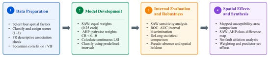
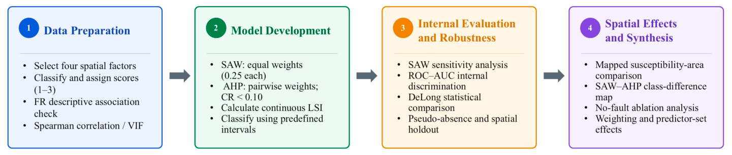
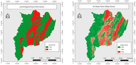
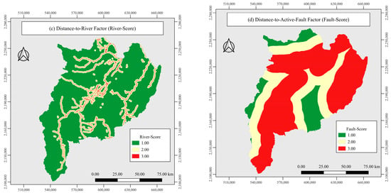
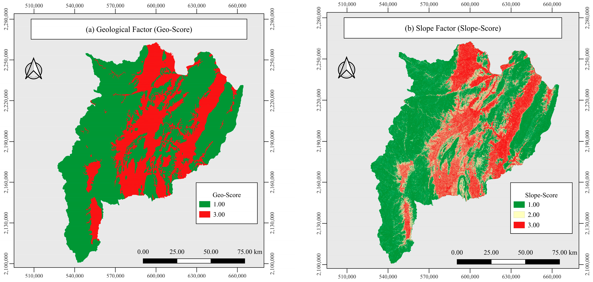
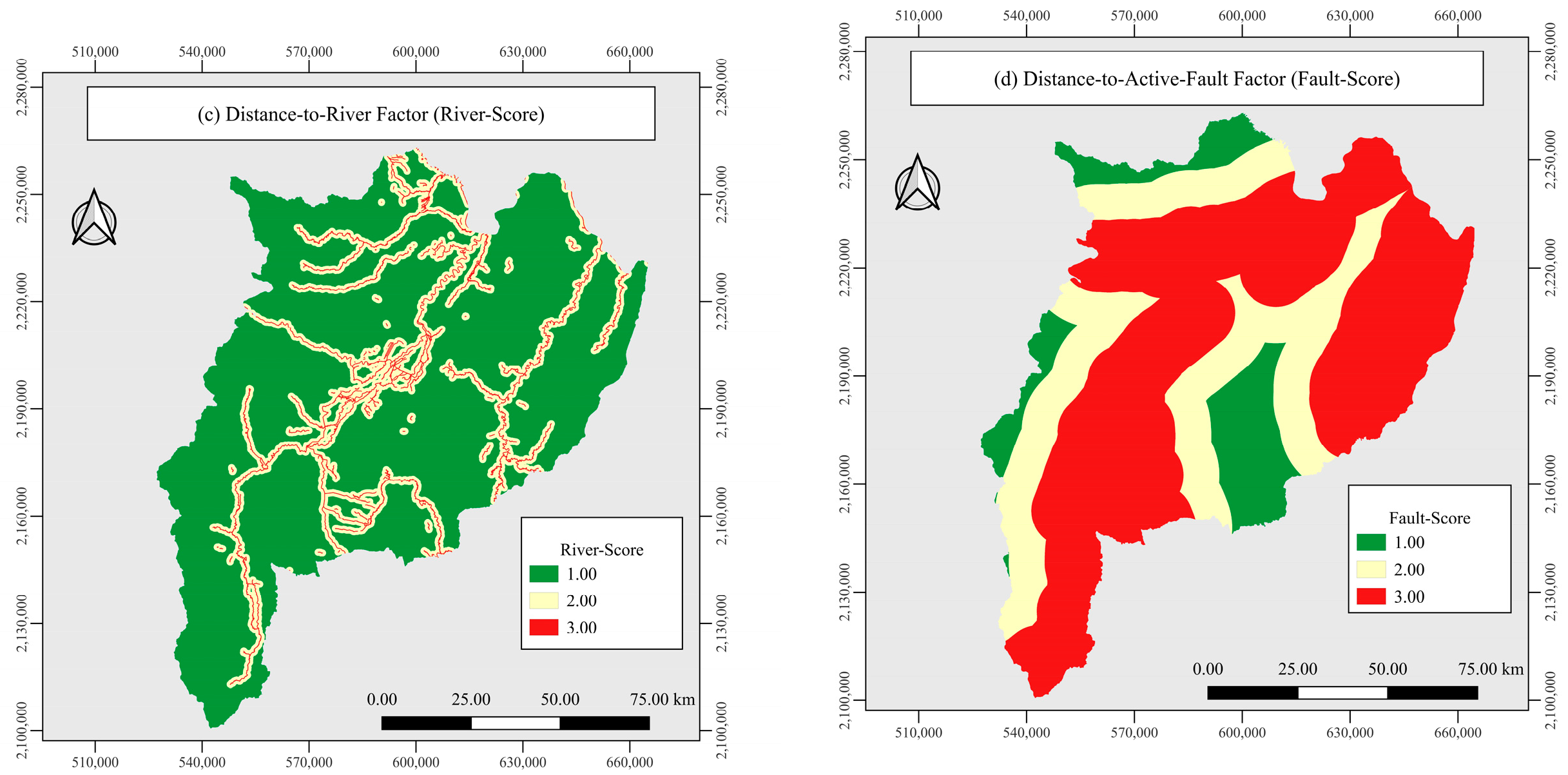
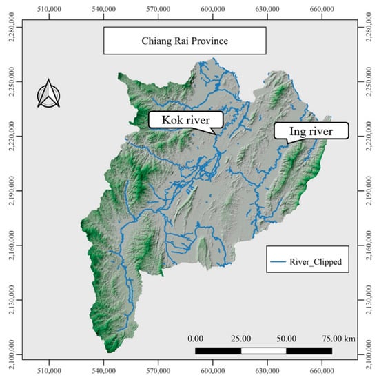
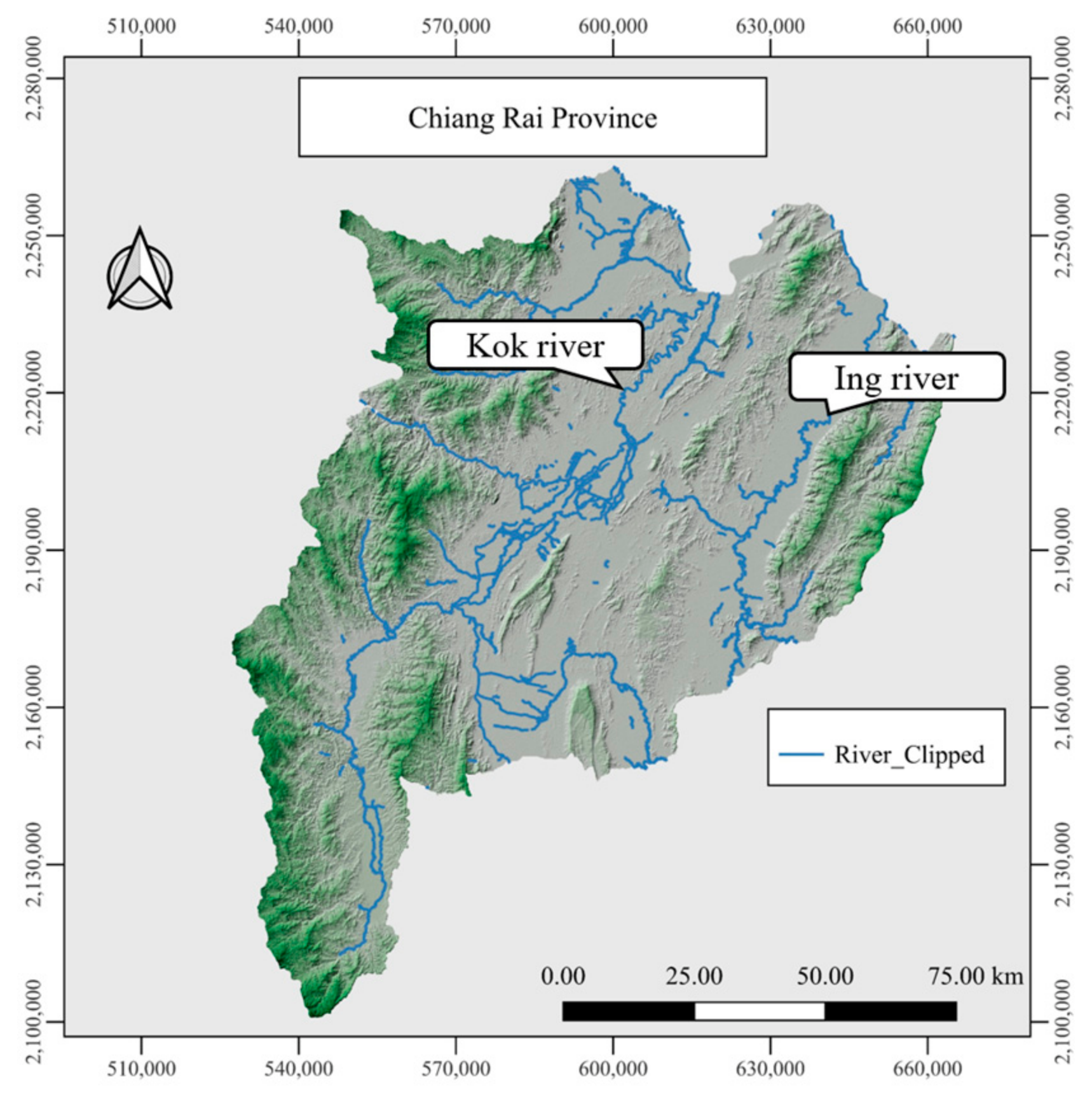
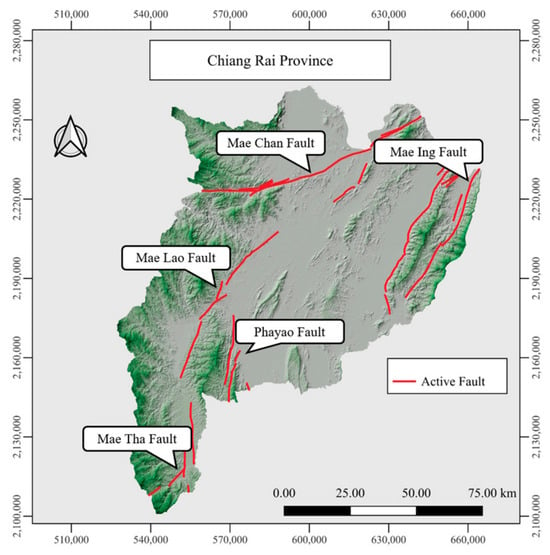
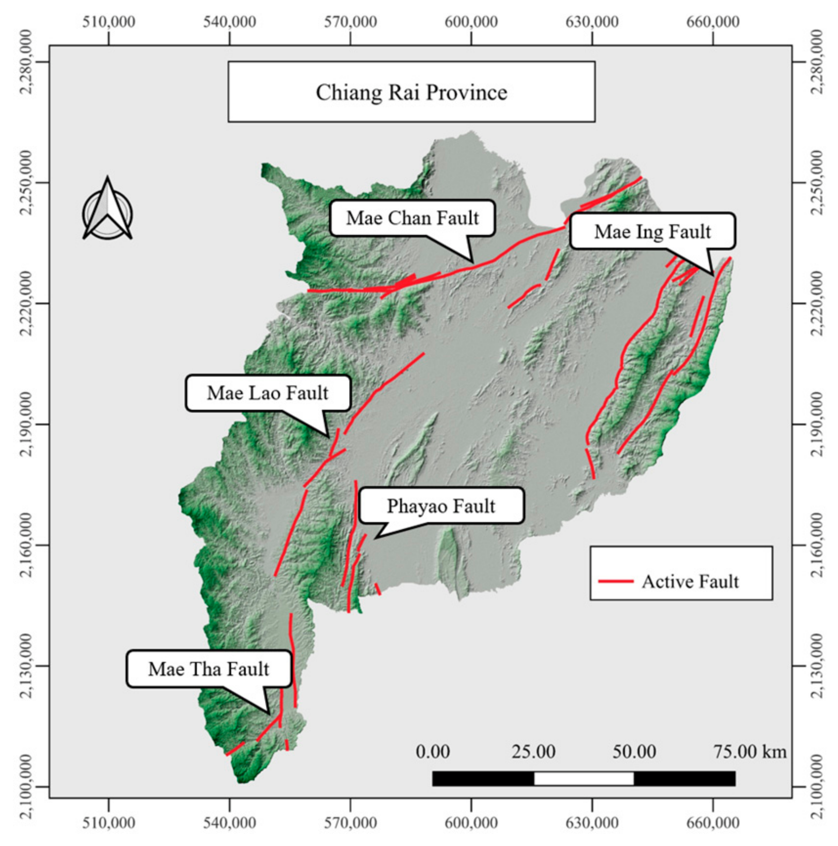
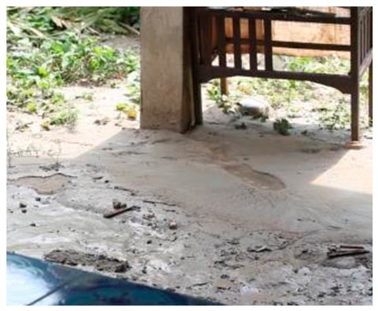
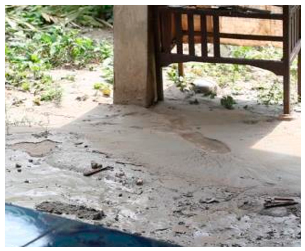
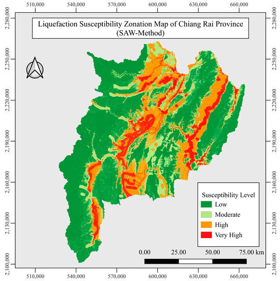
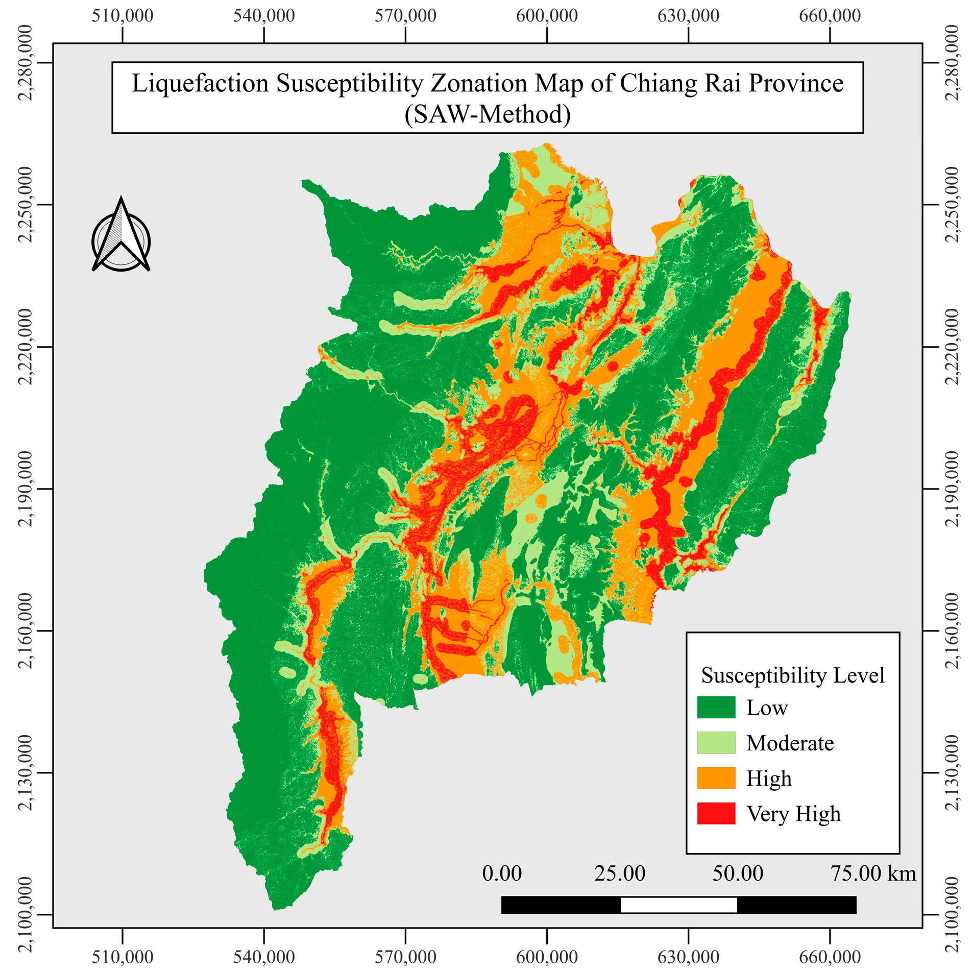
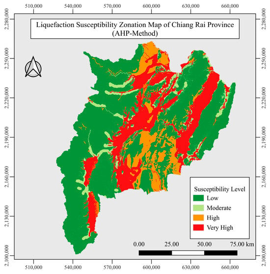
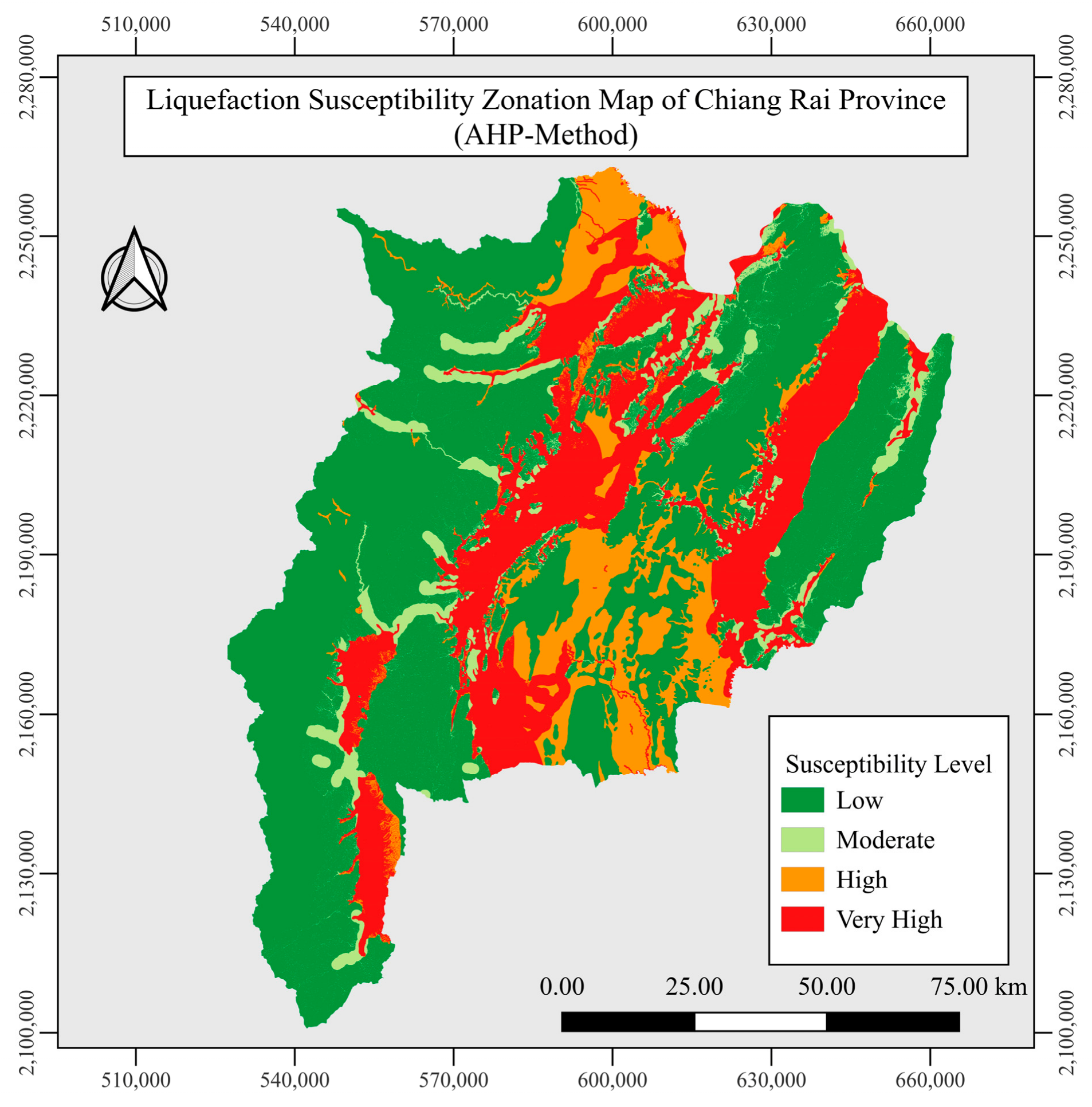
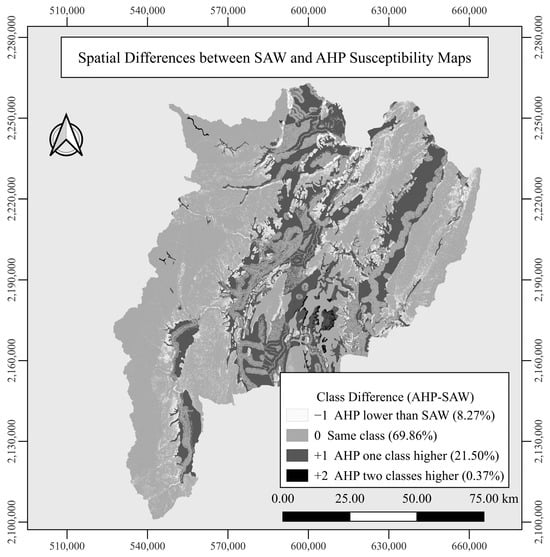
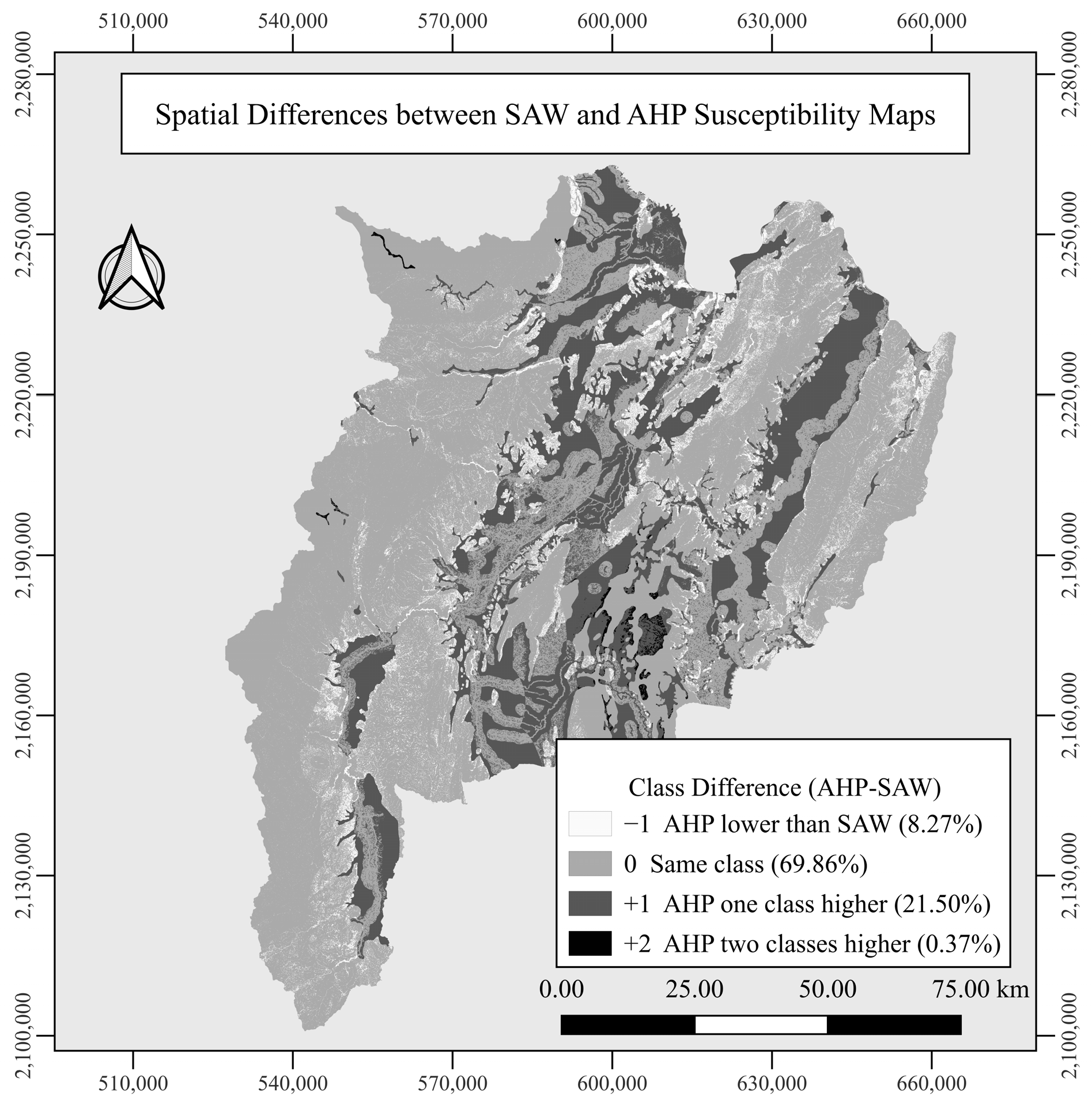
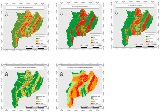
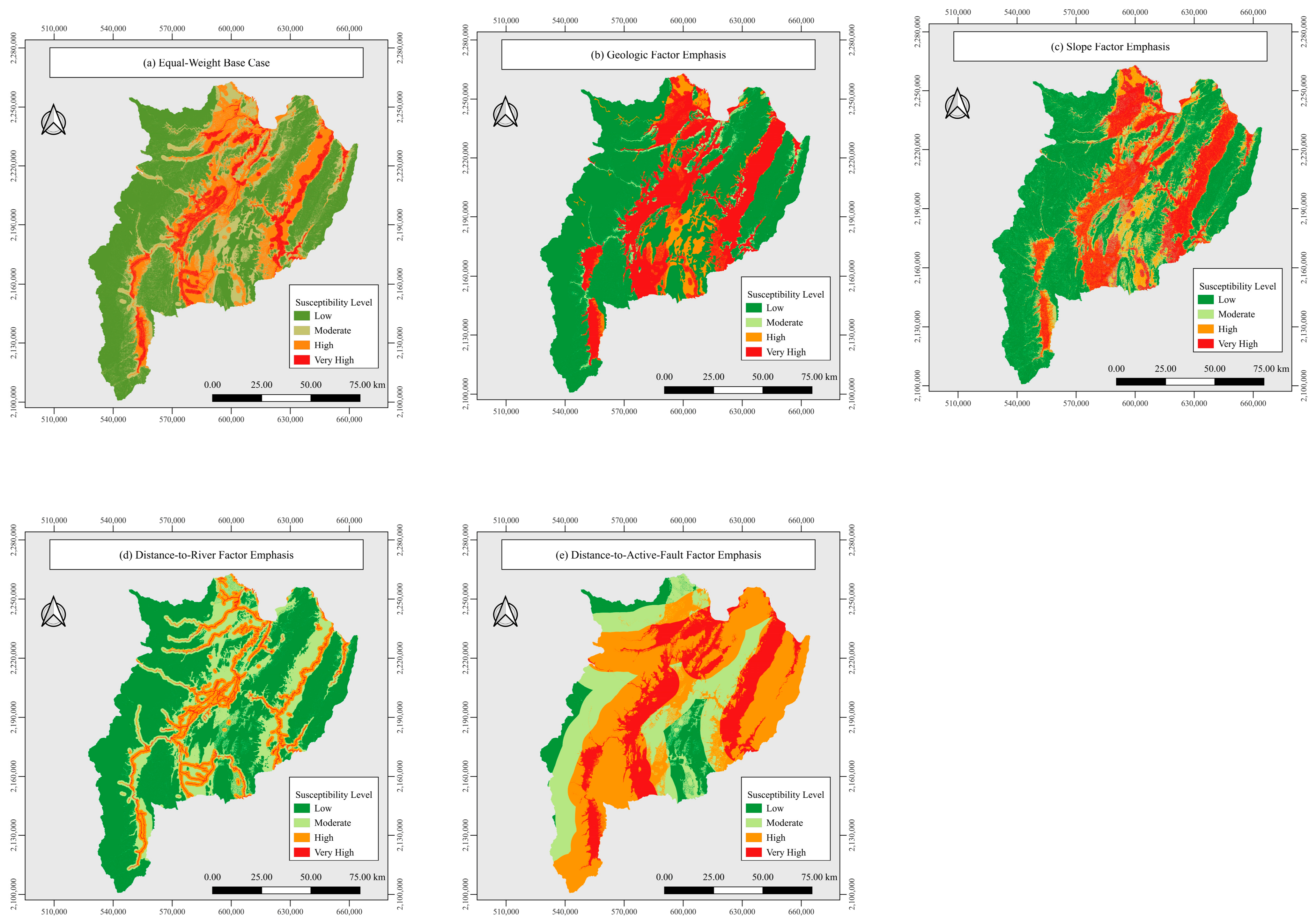
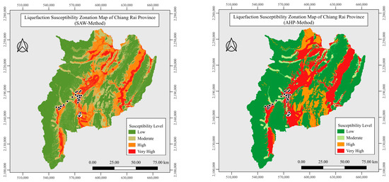
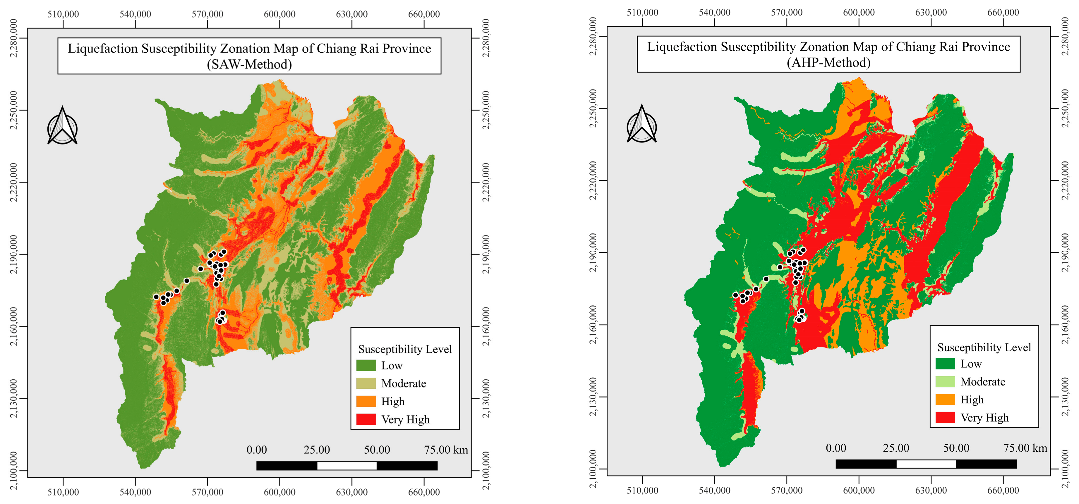
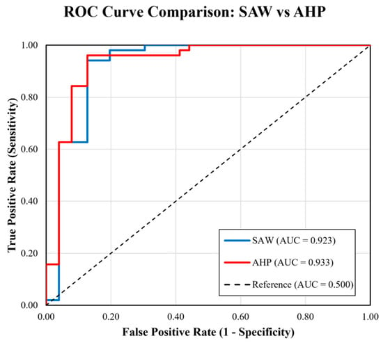
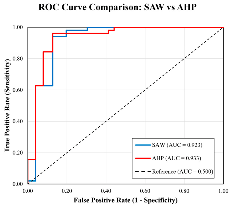

Disclaimer/Publisher’s Note: The statements, opinions and data contained in all publications are solely those of the individual author(s) and contributor(s) and not of MDPI and/or the editor(s). MDPI and/or the editor(s) disclaim responsibility for any injury to people or property resulting from any ideas, methods, instructions or products referred to in the content. |
© 2026 by the authors. Licensee MDPI, Basel, Switzerland. This article is an open access article distributed under the terms and conditions of the Creative Commons Attribution (CC BY) license.