


Abstract
Accurate mapping of Soil moisture (SM) is essential for effectively monitoring agricultural drought. However, the coarse spatial resolution of passive microwave products, including the 9 km Soil Moisture Active Passive (SMAP) retrievals, limits their effectiveness at regional and local scales. To address this limitation, three machine learning-based downscaling frameworks were compared to improve SMAP SM resolution from 9 km to 1 km over Békés County, Hungary. The study period covered the growing seasons (April to October) from 2020 to 2023. A set of multi-temporal MODIS-derived variables, including vegetation indices (NDVI, EVI), daytime and night-time land surface temperature, and evapotranspiration, along with land cover classification and topographic elevation, were combined as auxiliary predictor variables. Three machine learning algorithms, Random Forest (RF), Extreme Gradient Boosting (XGBoost), and Gradient Boosting Machine (GBM), were trained and evaluated. The results showed that (1) the RF model had the highest accuracy during the testing (R2 = 0.71, RMSE = 0.0295 m3/m3) phase and validation against four in situ monitoring stations with confirmed reliable SM estimation at the local scale; (2) daytime LST was the most important predictor in all models, underscoring the strong thermal–moisture coupling that governs surface SM dynamics; and (3) the validated RF model produced 1 km Standardized Soil Moisture Index (SSI) maps that effectively captured inter-annual drought variability, identifying the severe drought of July 2022. Overall, this study presents a downscaling approach for generating high-resolution SM data suitable for Central European agricultural environments. The resulting 1 km SM and SSI products provide valuable tools for decision-makers to enhance planning during drought periods and reduce agricultural losses through improved irrigation scheduling.
1. Introduction
Soil moisture (SM) is a fundamental climate variable that affects land–atmospheric interactions and is essential for agricultural productivity and drought management [1,2,3]. In Central Europe, including the Czech Republic, Slovakia, Hungary, and Romania, climate change has altered precipitation patterns and increased evapotranspiration demand, leading to an SM deficit and more frequent agricultural droughts in recent decades [4,5,6]. Since crop growth and yield depend on soil water availability, SM deficit in the root zone can significantly reduce yields and threaten food security [7,8]. Therefore, accurate, spatially detailed monitoring of SM is necessary for early drought detection, agricultural water management, and irrigation planning.
SM levels can be estimated using in situ measurements and remote sensing (RS) technologies [9]. However, traditional in situ SM measurements mostly rely on manual, point-scale monitoring stations and cannot capture continuous, large-scale spatial patterns of water content; they remain essential for calibrating and validating indirect measurements [10,11,12]. To overcome these limitations, remote sensing has been increasingly used for large-scale monitoring [13,14,15].
In recent decades, RS techniques have been used to obtain SM information from optical, thermal, and microwave sensors by utilizing the electromagnetic spectrum across several spatial and temporal scales [16]. Among the available RS technologies, microwave is the most suitable option due to its ability to penetrate cloud cover and operate independently of sunlight [17]. Microwave RS techniques indirectly measure the near-surface SM at depths of less than 5 cm by analyzing the relationship between volumetric water content and the dielectric properties of the soil. These sensors are classified as active (using their own energy source) or passive (using the sun’s energy) radar based on their signal source [18,19]. The Soil Moisture Active Passive (SMAP) mission carries an L-band passive microwave sensor that provides accurate SM retrievals worldwide every two to three days, but at coarse spatial resolutions of 36 km and 9 km [20,21]. However, these coarse-resolution satellites average the SM signal over large areas that include different crops and soil types, thereby losing details of farming practices [22]. These products suit continental- and global-scale studies but not regional applications, including small, heterogeneous agricultural fields that require higher spatial resolution; thus, downscaling algorithms can enhance the products to 1 km [1,23]. To obtain finer-resolution SM information from coarse microwave products, downscaling approaches commonly leverage optical and thermal infrared RS observations as auxiliary data, exploiting the physical relationships among SM, land surface temperature (LST), and vegetation parameters [24].
Furthermore, single-source data may have spatial and temporal gaps due to satellite orbits and sensor limitations [25]. The accuracy of SM retrieval depends on land surface characteristics, such as vegetation cover, land use, and topography. Therefore, data fusion methods can synergistically combine multiple data sources to enhance accuracy and provide more comprehensive datasets through downscaling [26,27]. Data from the Moderate Resolution Imaging Spectroradiometer (MODIS), including vegetation indices (NDVI and EVI), LST, and evapotranspiration (ET), have been widely used as auxiliary predictor variables for SMAP SM downscaling [1,28,29]. Among these, LST and vegetation indices have consistently been identified as the most influential predictors due to their strong relationships with surface energy balance and soil water content [1,29,30]. However, the relationship between these land surface variables and SM is nonlinear and complex. As a result, traditional statistical methods are insufficient and underscore the need for advanced machine learning algorithms to capture these interactions effectively [31,32].
Downscaling SM satellite methods are categorized into physically based, statistical, and ML approaches. Each approach has its merits and limitations. Physical models perform well under bare-soil conditions based on rigorous equations and require extensive input data. Disaggregation based on Physical And Theoretical scale Change (DISPATCH) is a representative physical model and relies on the physical link between soil evaporative efficiency and LST, as drier soil heats up faster than wetter soils. [33,34]. This method offers strong physical consistency but depends on detailed inputs, such as soil hydraulic properties, and struggles under dense vegetation [35,36]. Conventional statistical approaches are empirical methods that use mathematical relationships between coarse-resolution satellite data and high-resolution environmental variables [37]. These methods rely on regression models or the LST vegetation index triangle method, such as the Temperature Vegetation Dryness Index (TVDI), but are limited in capturing non-linear relationships [38]. However, their accuracy depends on site-specific environmental conditions and requires local calibration, which limits their generalizability across diverse agroecological conditions [9].
To overcome these limitations, machine learning methods are commonly used to scale coarse-resolution SM data to finer resolution [39,40]. By using ML algorithms and combining data from multiple sources (optical, thermal, and microwave), the complex nonlinear interactions among SM, optical, thermal, and microwave data can be effectively modeled [41]. Among the available machine learning algorithms, Random Forest (RF) and Gradient Boosting Machine (GBM) have shown strong performance in downscaling SM and achieving higher spatial resolutions [42,43,44]. Wang et al. [45] applied RF to downscale SMAP data to 1 km resolution over China’s Loess Plateau, demonstrating good agreement with in situ measurements (R = 0.654). In another study, Wei et al. [46] successfully downscaled SMAP from 36 km to 1 km over the Tibetan Plateau during 2015–2017, using Gradient Boosting Decision Tree regression with MODIS and DEM data. While individual ML methods have been effectively demonstrated, ensemble approaches can combine multiple algorithms to achieve better performance. Based on these results, assessing the performance of various algorithms in SM downscaling across diverse regions and climates is essential to determine the accuracy of high-resolution products for agricultural drought monitoring.
To monitor agricultural drought, higher-resolution SM data can be combined with advanced drought indices to identify local drought conditions [47,48]. The Standardized Soil Moisture Index (SSI) is a common drought indicator that measures drought severity by comparing SM anomalies to a long-term average [49]. Although machine learning models have shown good results for downscaling soil moisture, their accuracy at a 1 km resolution with downscaled data has not been fully assessed. High-resolution SM-based drought monitoring remains limited in the Central European Plain. Current regional systems, including the Czech Drought Monitoring system, primarily use modeled soil water balance with coarse microwave data [50]. This limitation is significant as agricultural land in this region is highly fragmented. Average field block size ranges from approximately 5 hectares in Poland to 12 hectares in the Czech Republic and 8 to 10 hectares in Hungary [51]. In Hungary, microwave RS has played a limited role in agricultural drought monitoring because passive sensors such as SMAP provide coarse spatial resolution. This limitation persists despite the region’s high drought vulnerability and its reliance on drought-sensitive crops such as maize, wheat, and sunflower [52,53,54].
This study aims to (a) generate 1 km resolution SM data for Békés County, Hungary, by downscaling the SMAP coarse-resolution product using three categories of predictor variables: dynamic variables (NDVI, EVI, daytime and nighttime LST, and ET), land cover type, and topographic elevation; (b) evaluate the generalization and predictive performance of three machine learning models, including Random Forest, XGBoost, and Gradient Boosting models, across temporal and spatial scales, with validation being based on in situ measurements from four agricultural monitoring stations collected between 2020 and 2023; and (c) apply the best-performing model to calculate the SSI for finer-resolution monitoring of agricultural drought.
2. Materials and Methods
2.1. Study Area
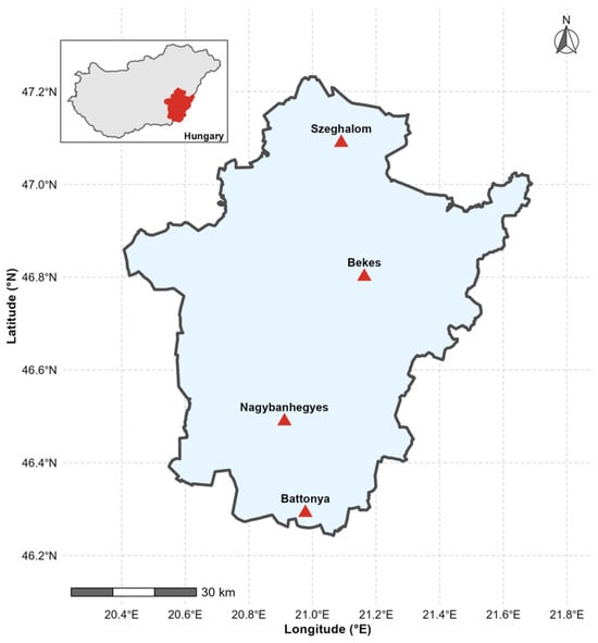
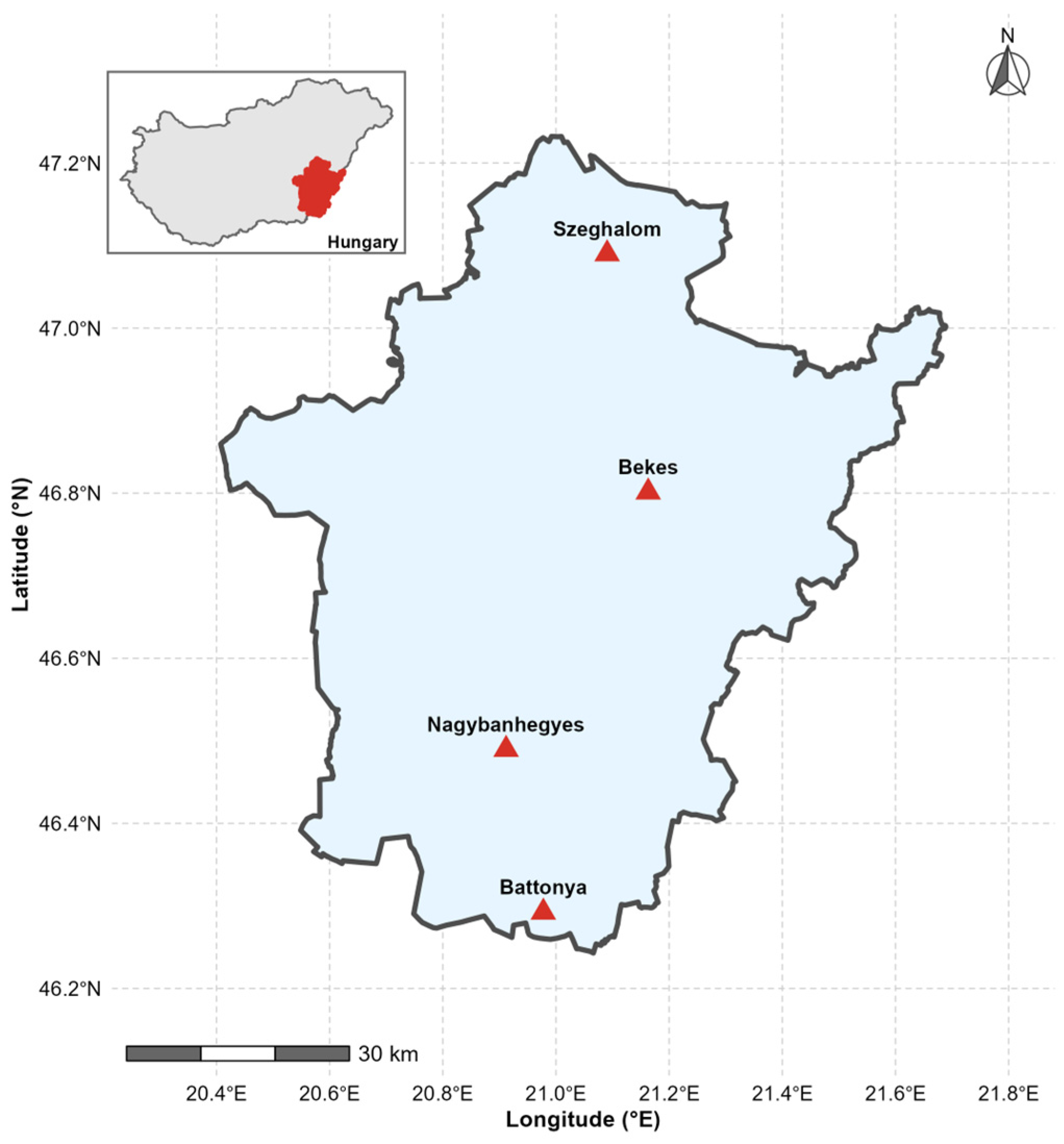
Our study was in Békés County, in the southeastern part of the Great Hungarian Plains (Alföld). It covers approximately 5600 km2. This region has predominantly flat topography with elevations from 80 to 100 m above sea level. Fertile Chernozem soils dominate the area, with some Phaeozem soils in the Körös River floodplain, making it one of Hungary’s most productive agricultural regions [55]. The region has a continental climate with hot summers and increasing susceptibility to seasonal drought. Hungary experienced a severe compound heatwave and drought in 2022 [56]. Water-related challenges present substantial risks to the region’s intensive agricultural production, which occupies approximately 80% of the land area and includes major crops such as maize, winter wheat, sunflower, and rapeseed. [57]. Four SM monitoring stations operated by the Hungarian National Water Directorate (OVF) were selected for this study—Békés, Szeghalom, Nagybánhegyes, and Battonya—with continuous volumetric SM measurements (Figure 1). The average size of soil blocks typically ranges from 8 to 10 ha, causing challenges for operational SM monitoring from coarse-resolution satellite products [51]. Therefore, reliable field-scale SM information is crucial for irrigation scheduling and drought monitoring in agricultural regions. These characteristics make Békés County a suitable test site for assessing multi-sensor data fusion approaches.
Figure 1.
Study area in Békés County, Southeastern Hungary. The red triangles represent the stations location—Data source: “Országos Vízügyi Főigazgatóság (OVF)” [58].
2.2. Framework and Data Collection
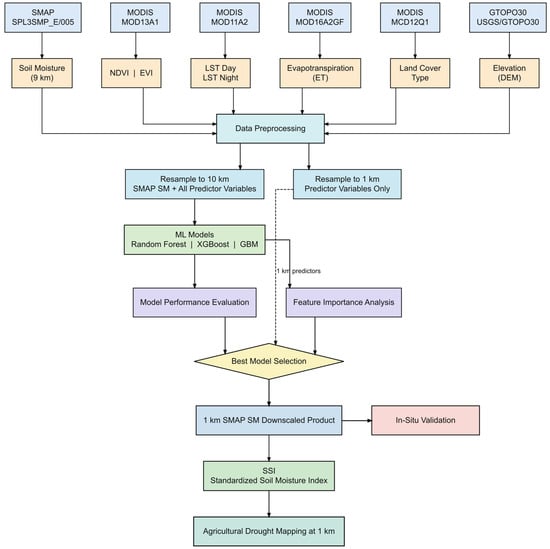
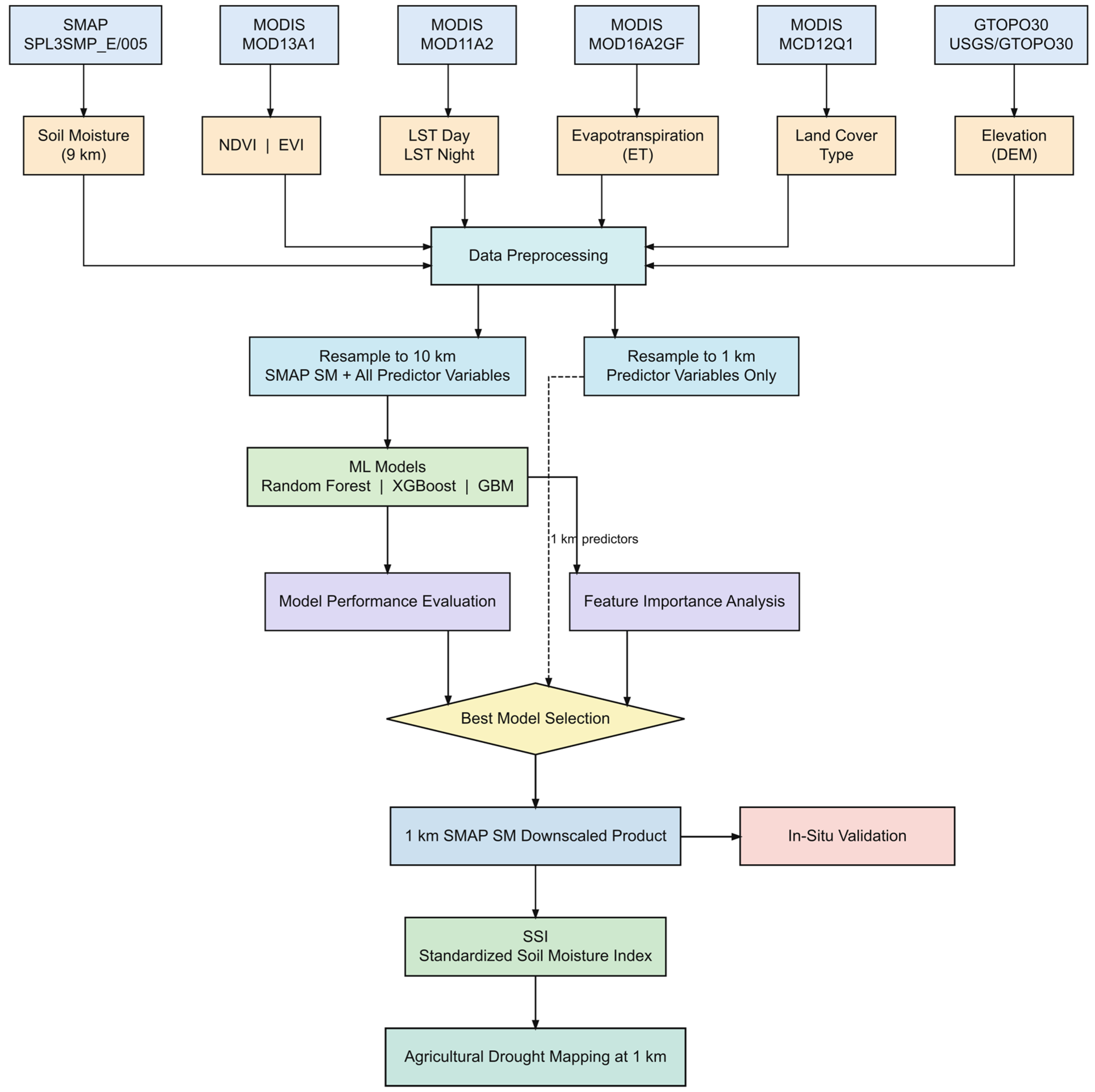
The framework of our study is shown in Figure 2. The workflow integrates multi-source satellite datasets. The procedure is structured into six phases and described in detail in the following subsections.
Figure 2.
Methodological framework. The dashed line shows a 1 km predictor applied to the trained model.
2.2.1. In Situ Soil Moisture Measurement Data
Capacitive sensors measure volumetric soil moisture by detecting changes in the soil’s dielectric permittivity, which depends on water content [59]. At each of the OVF drought monitoring stations, capacitive soil moisture and temperature sensors sensors (Decagon 5TM or METER Teros11, depending on installation date) have been operated at different depths (10, 20, 30, 45, 60 and 75 cm), recording hourly volumetric SM data [58]. For the purpose of our study we have utilized the data from 10 cm depth for the four selected stations. The characteristics of each station are listed in Table 1. For this study, we used SM data (m3/m3) from the growing seasons (April–October) between 2020 and 2023 from the OVF database. We averaged the hourly SM data to the monthly scale for model validation.
Table 1.
Features of the in situ soil moisture monitoring stations—Data source: (OVF) [58].
2.2.2. MODIS Data
Three MODIS products were used in this study: MOD13A1 vegetation index data at 500 m resolution every 16 days, including both Normalized Difference Vegetation Index (NDVI) and Enhanced Vegetation Index (EVI) [60]. MOD11A2 LST data with a 1 km resolution every 8 days, both LST_Day and LST_Night [61], and MOD16A2GF ET data with a resolution at 500 m every 8 days [62].
Daytime LST was selected as the primary thermal predictor because it is sensitive to SM dynamics via surface energy balance processes [1,24]. Nighttime LST was also included to capture the diurnal temperature range and provide additional information on soil thermal properties. NDVI and EVI were selected as indicators of vegetation phenology and canopy density. ET was included to directly capture the water flux between the land surface and atmosphere, as this process is closely associated with SM availability. MODIS data were acquired from the Google Earth Engine (GEE) platform and aggregated into monthly composites from April to October, 2020 to 2023.
2.2.3. Topographic Data
Elevation data were sourced from the USGS GTOPO30 Digital Elevation Model, which provides approximately 1 km spatial resolution [63]. Elevation was used as a static variable to capture topographic influences on soil moisture, such as drainage, runoff, and solar radiation.
2.2.4. Land Cover Data
Land cover type was determined using the MODIS Terra+Aqua MCD12Q1 product at a 500 m spatial resolution, applying the IGBP classification scheme (LC_Type1) [64]. The dominant land cover type for each pixel was identified by calculating the annual land cover mode over the study period. Examination of the study area indicated that Békés County is primarily classified as cropland (IGBP Type 12), which aligns with its agricultural profile.
2.2.5. SMAP L3 Radiometer
The SMAP Level-3 Enhanced product was used as the baseline for coarse-resolution soil moisture, providing data at a 9 km scale. The SPL3SMP_E Version 5 product [65] delivers daily global coverage at 9 km resolution, updates every 2–3 days using an L-band (1.41 GHz) passive microwave radiometer, and estimates volumetric water content in the top 5 cm of the soil profile (in m3/m3) [20]. We used only morning descending orbit acquisitions (approximately 06:00 local time) because they best represent near-equilibrium SM conditions before daytime thermal forcing [66]. Table 2 represents a list of all satellite products used as predictors and target variables in this study.
Table 2.
List of products used for downscaling in this study.
2.3. Data Preprocessing
We obtained all satellite datasets directly from their respective source collections in Google Earth Engine: SMAP SPL3SMP_E (the morning/descending overpass band only), MOD13A1 (NDVI, EVI), MOD11A2 (daytime and nighttime LST), MOD16A2GF (ET), MCD12Q1 (land cover), and the GTOPO30 DEM. For each variable and calendar month in the study period, we combined all available native-resolution images from that month into a single monthly composite using a pixel-wise temporal mean. The MODIS products used are pre-processed composites that incorporate quality screening at the source. For example, MOD16A2GF gap-fills low-quality ET retrievals, and MOD13A1 and MOD11A2 apply per-pixel reliability screening during their respective 16-day and 8-day compositing intervals. Pixels flagged as invalid or cloud-contaminated in the source product contain no data, and Earth Engine’s reducer automatically excludes them from the monthly mean, rather than averaging them as erroneous values. This monthly averaging step further reduces the influence of any residual gaps, as multiple sub-monthly composites contribute to each final monthly image. To avoid errors from frozen-soil conditions in SMAP microwave retrievals, we limited temporal aggregation to the growing season (April to October). In total, this process resulted in 28 monthly composites over the study period from 2020 to 2023.
Predictor variables were spatially resampled in GEE to two target resolutions: (i) 10 km for model training, matching the native SMAP spatial resolution of approximately 9 km; and (ii) 1 km for spatial prediction. Bilinear resampling was used for continuous variables (LST, NDVI, EVI, ET, and elevation), and nearest-neighbor resampling was used for categorical variables (land cover type). The final training dataset included approximately 538,061 spatiotemporal observations, each containing seven predictor variables and one target variable (SMAP soil moisture).
Training data were extracted by co-locating SMAP soil moisture observations with corresponding predictor values at the same spatial location and within the same temporal window. To ensure data quality, we excluded pixels with missing values due to cloud contamination in MODIS optical data and used only cloud-free observations for model training. The final dataset was randomly split into 80% for training and 20% for testing to evaluate model generalizability.
2.4. Machine Learning Models
2.4.1. Random Forest Regression on Soil Moisture Data
We used Random Forest [67] for soil moisture downscaling. It is an ensemble method that builds many decision trees from bootstrapped subsets of the training data. At each split, only a randomly selected subset of predictor variables is considered. This decorrelates the trees and helps the model generalize better than a single decision tree. The final prediction is the average across all trees in the ensemble.
The relationship between SM and the satellite-derived predictors is nonlinear, and RF captures this without requiring us to specify a functional form in advance. It also handles multi-source data without requiring explicit feature selection beforehand, and it produces built-in importance rankings that let us assess each predictor’s contribution directly, which we used in the MDI analysis. Just as importantly, RF tends to remain robust even when predictors are correlated, which mattered here given the collinearity we observed between LST and the vegetation-related variables. At each node split, RF selects the optimal split from a random subset of predictors. This approach prevents any single group of correlated variables from dominating every split, thereby decorrelating individual trees and reducing the influence of redundant predictors on the ensemble’s overall predictions [68,69].
2.4.2. Gradient Boosting Regression
Gradient Boosting (GBM) [70] constructs an ensemble of decision trees sequentially, in contrast to the parallel construction used by Random Forest. Each new tree is trained to correct the residual errors of the previous trees. Instead of employing bagging, Gradient Boosting utilizes an additive strategy, fitting each successive tree to the gradient of the loss function with respect to current predictions. This sequential correction can improve accuracy compared to purely parallel ensembles; however, it also increases the risk of overfitting, necessitating careful regularization. GBM was included in the comparison to evaluate whether this sequential, error-correcting approach could outperform Random Forest’s bagging strategy for soil moisture downscaling. Additionally, the analysis aimed to determine whether feature importance rankings remained consistent across fundamentally different ensemble strategies, specifically parallel versus sequential methods, or whether the choice of algorithm influenced which predictors appeared most influential.
2.4.3. Extreme Gradient Boosting
XGBoost [70] is a widely used gradient boosting implementation, designed for computational efficiency and scalability on large, high-dimensional datasets through a combination of algorithmic and system-level optimizations [71]. Like other gradient boosting methods, it builds trees sequentially but includes built-in L1 and L2 regularization and supports parallel computation, which together improve generalization compared with standard gradient boosting machine (GBM) implementations. Its demonstrated effectiveness in remote sensing applications is largely due to its ability to model nonlinear relationships in complex, high-dimensional feature spaces while remaining computationally tractable at scale [72]. XGBoost gradient-boosted trees can handle multicollinearity among predictors. Tree node splitting in decision trees relies on reducing node impurity measures. In XGBoost, splitting is determined by a metric that quantifies a feature’s distribution. When correlated variables exist in the input feature space, the decision tree typically selects only one variable for splitting [73]. Subsequent splits use uncorrelated variables, since correlated variables provide minimal information gain. Because boosted trees in XGBoost employ an ensemble of decision trees, the algorithm inherently mitigates overfitting, a common issue when a single decision tree is applied to multicollinear variables [74]. In this study, we implemented XGBoost (version 3.4.1) using the open-source XGboost Python library.
All data acquisition and preprocessing were conducted on the Google Earth Engine (GEE) cloud platform via its Python API, accessed through Google Colab [75,76].
2.5. Model Implementation
We trained and implemented two machine learning algorithms, RF and GBM, using the scikit-learn (version 1.6.1) Python library [77], and implemented XGBoost using the XGboost library [71]. We trained the models on the 80% training subset.
All models were trained on an 80% training subset. We evaluated hyperparameters for each model using sensitivity analysis with 3-fold cross-validation, evaluated by R2, across a limited set of candidate configurations for each algorithm (Supplementary Table S1). The random forest (RF) model was trained with 100 decision trees (n_estimators = 100, max_depth = None). The XGBoost model used 5000 boosting iterations and a learning rate of 0.05 (n_estimators = 5000, learning_rate = 0.05). The gradient boosting machine (GBM) model was configured with 500 boosting iterations, a learning rate of 0.05, and a maximum tree depth of 5 (n_estimators = 500, learning_rate = 0.05, max_depth = 5). All models used a fixed random seed (random_state = 42) to ensure reproducibili. Each model learns a statistical mapping from the high-resolution predictor variables to soil moisture, which can be expressed as:
where is the estimated SM at 1 km resolution, and f represents the trained machine learning function. Once this mapping is created, 1 km SM estimates can be generated directly from the predictor variables.
2.6. Agricultural Drought Monitoring
After SM downscaling, SSI [78] was calculated to assess agricultural drought across the study area at 1 km resolution. To produce a robust climatological baseline, we applied the trained RF model to historical predictor datasets during the growing season (April to October) from 2004 to 2023. This process reconstructed a continuous 20–year monthly SM record at 1 km resolution. The resulting extended record provided sufficient temporal depth to derive reliable long-term monthly statistics at the pixel level.
For each pixel and each calendar month, the long-term mean (μm) and standard deviation (σm) were computed across all available years, and the SSI was then calculated following [78] as:
where θm is the reconstructed 1 km SM for month m. Positive SSI values indicate normal conditions, while negative values show SM deficits. The drought category was classified according to the thresholds presented in Table 3.
Table 3.
Soil Moisture drought classification based on SSI scheme.
2.7. Validation and Performance Assessment
We used four metrics to assess how well the ML models predicted soil moisture. These metrics were the coefficient of determination (R2), Root Mean Square Error (RMSE), Unbiased Root Mean Square Error (ubRMSE) [20], and Mean Absolute Error (MAE). R2 indicates the proportion of variance explained by the model, while RMSE and MAE quantify the average magnitude of prediction errors in m3/m3. The ubRMSE isolates the random error component by removing systematic bias and serves as the primary benchmark for accuracy in SM validation. For all metrics, values closer to zero for RMSE, ubRMSE, and MAE, and closer to 1 for R2, indicate better model performance.
The calculation formulas are as follows:
where yi is the observed SMAP soil moisture, is the model-predicted value, is the mean of observed values, and n is the number of test samples.
3. Results
3.1. Soil Moisture Patterns
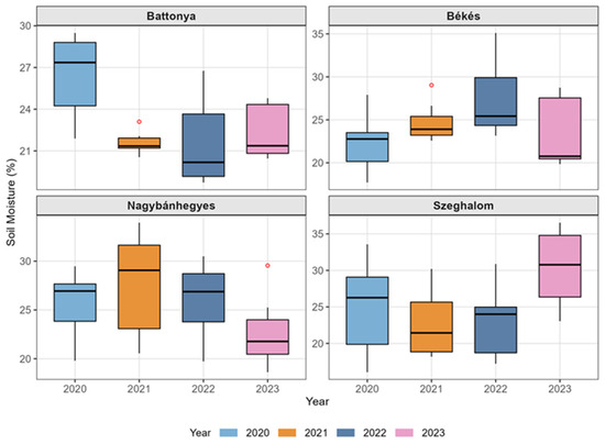
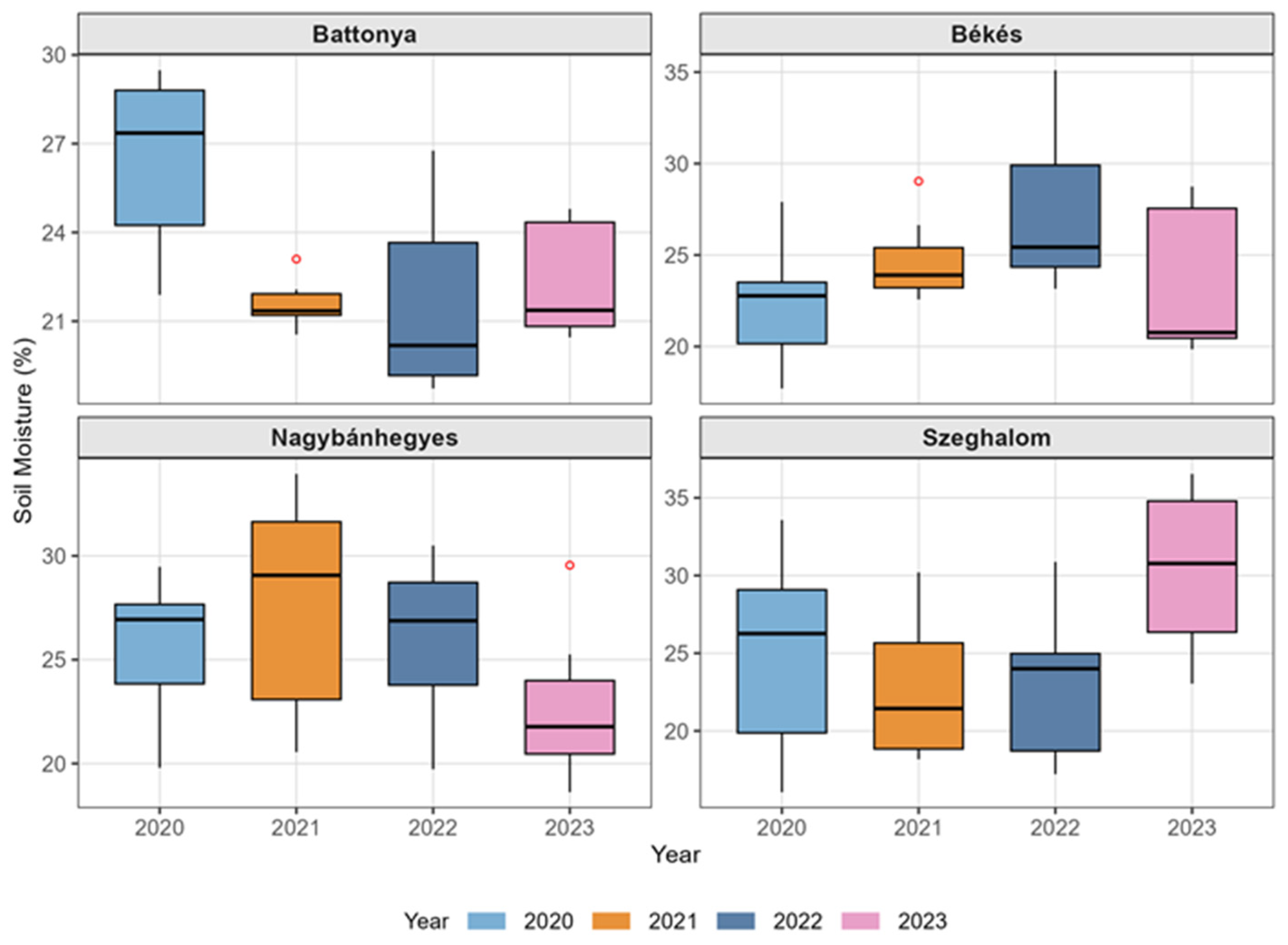
Box plots of SM data from our four stations at a depth of 10 cm during the growing season from 2020 to 2023 are shown in Figure 3. At Battonya station, SM dropped sharply from about 27% in 2020 to a low of about 20% in 2022, then increased slightly to about 22% in 2023. This made Battonya the station with the lowest SM values during the study. At Békés station, SM rose steadily from about 22% in 2020 to a peak of about 26% in 2022, then fell to its lowest value of about 21% in 2023. Nagybánhegyes had its highest median SM in 2021 at about 29%, then fell moderately to about 27% in 2022 and more sharply to about 22% in 2023. Szeghalom station had the biggest swings, with SM being at its lowest in 2021 (about 22%) and then jumping to its highest in 2023 (about 30%), which was the highest single median among all stations and years. In summary, Battonya showed a clear drying trend through 2022, while the other stations had more varied and complex patterns. This highlights how SM changes differently across Békés County.
Figure 3.
Soil moisture at 10 cm depth across four ground stations in Békés County, Hungary, during growing seasons (April–October, 2020–2023). Red dots represent statistical outliers.
3.2. Feature Importance Analysis
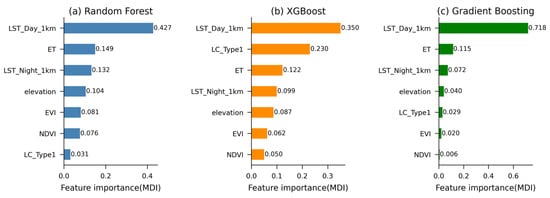
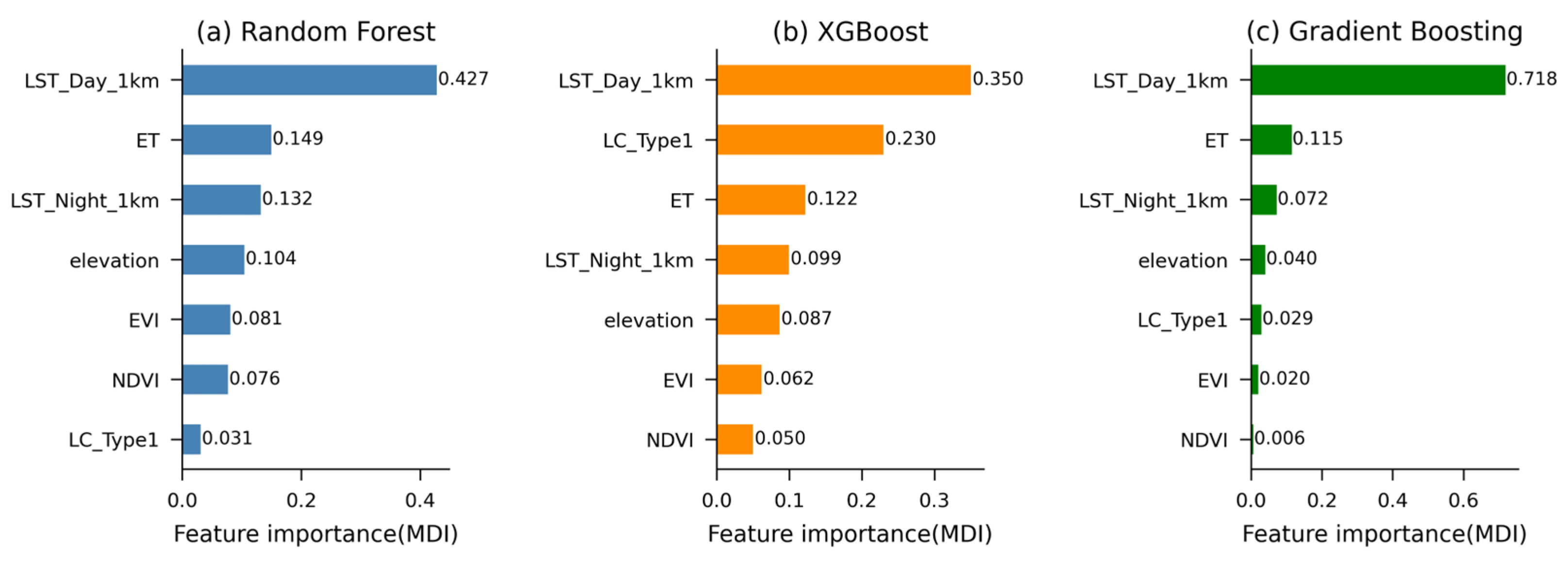
We ranked each predictor’s contributions to the tree-based model’s performance via the Mean Decrease Impurity (MDI) method [67,72,79]. MDI measures how much each predictor reduces node impurity, averaged over all trees in the ensemble [33]; higher values indicate greater influence on model predictions. Figure 4 compares each predictor’s MDI-based importance ranking across three models. Across all models, LST_Day_1km ranked as the most important predictor, with importance values of 0.428, 0.352, and 0.718 for RF, XGBoost, and Gradient Boosting, respectively. Evapotranspiration (ET) was the second most important predictor in RF (0.149) and Gradient Boosting (0.115), while land cover type (LC_Type1) ranked second in XGBoost (0.223). Nighttime LST (LST_Night_1km) consistently ranked third across all models, with importance values of 0.132, 0.099, and 0.072 for RF, XGBoost, and Gradient Boosting, respectively. Among vegetation indices, EVI was more important than NDVI across all models. LC_Type1 showed the lowest importance in RF (0.031) and Gradient Boosting (0.029), while NDVI showed the lowest importance in XGBoost (0.052) and Gradient Boosting (0.006). The distribution of feature importance differed notably between models. RF and XGBoost distributed importance more evenly across predictors, while Gradient Boosting concentrated 71.8% of total importance on LST_Day_1km alone.
Figure 4.
Feature importance (MDI) for (a) Random Forest, (b) XGBoost, and (c) Gradient Boosting models used for SMAP downscaling. Values are normalized to sum to 1.
3.3. Accuracy Comparison of ML Models
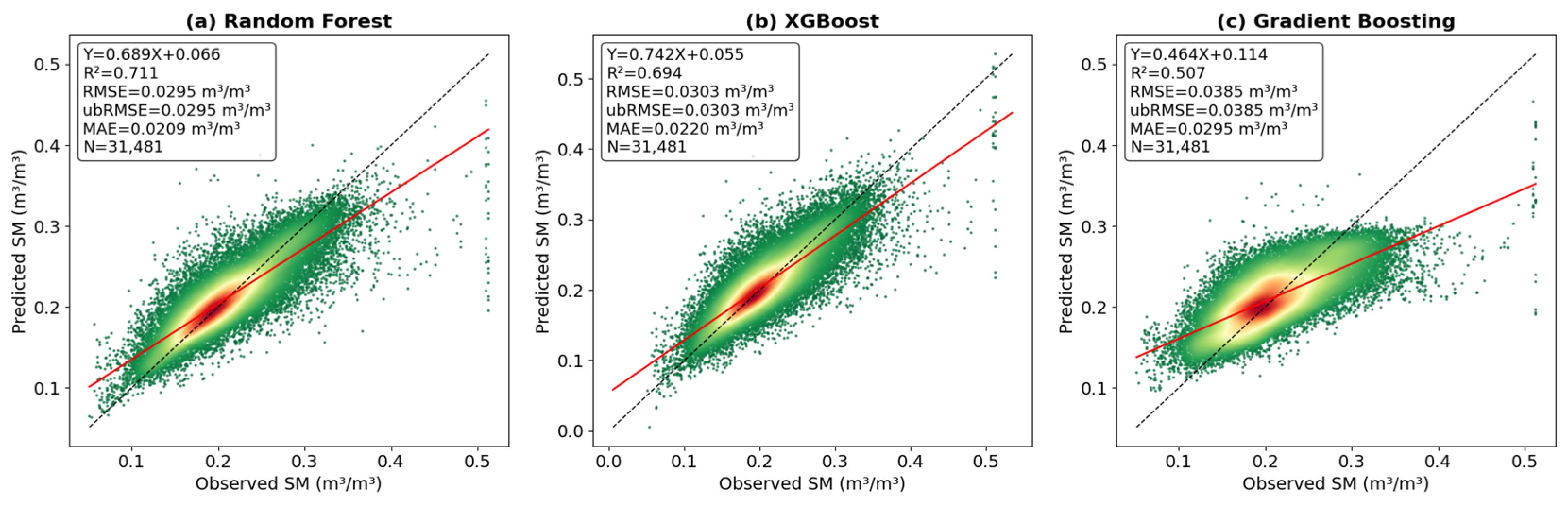
Table 4 presents test dataset performance results for the three ML models. Among the three models, Random Forest achieved the best overall performance, with R2 = 0.711, RMSE = 0.030 m3/m3, ubRMSE = 0.030 m3/m3, and MAE = 0.021 m3/m3, followed closely by XGBoost with R2 = 0.692 and ubRMSE = 0.030 m3/m3. Gradient Boosting showed comparatively weaker performance, with R2 = 0.507 and ubRMSE = 0.039 m3/m3, though still within an acceptable range for SM estimation. Both RF and XGBoost models’ accuracy confirmed the downscale model’s reliability, with targets of ubRMSE ≤ 0.04 m3/m3. However, RF was selected as the primary model for SM downscaling, as supported by the literature: Sang et al. [68] demonstrated that RF achieved R2 = 0.92 in a multimodal fusion framework and outperformed XGBoost (R2 = 0.76). Wang et al. [33] similarly reported that RF achieved the highest correlation (R2 = 0.654) with in situ measurements over China’s Loess Plateau. These results proved that RF provided accurate SM estimates across different regions.
Table 4.
Performance metrics of the three ML models on the tested dataset.
Figure 5 shows the point density scatter plots. The regression slopes for all models were below 1, indicating that the predicted SM range was narrower than the observed range. This pattern is common in ensemble regression models because they often predict values closer to the training data mean to reduce error [80]. The density plots showed that most predictions cluster around moderate SM values (0.15–0.30 m3/m3), that aligned with the common conditions in the training data during downscaling.
Figure 5.
Point density scatter plots of observed and predicted SM for (a) Random Forest, (b) XGBoost, and (c) Gradient Boosting models. The black dash and red lines are the 1:1 reference and the fitted regression line, respectively.
3.4. Spatial Distribution of Downscaled SM
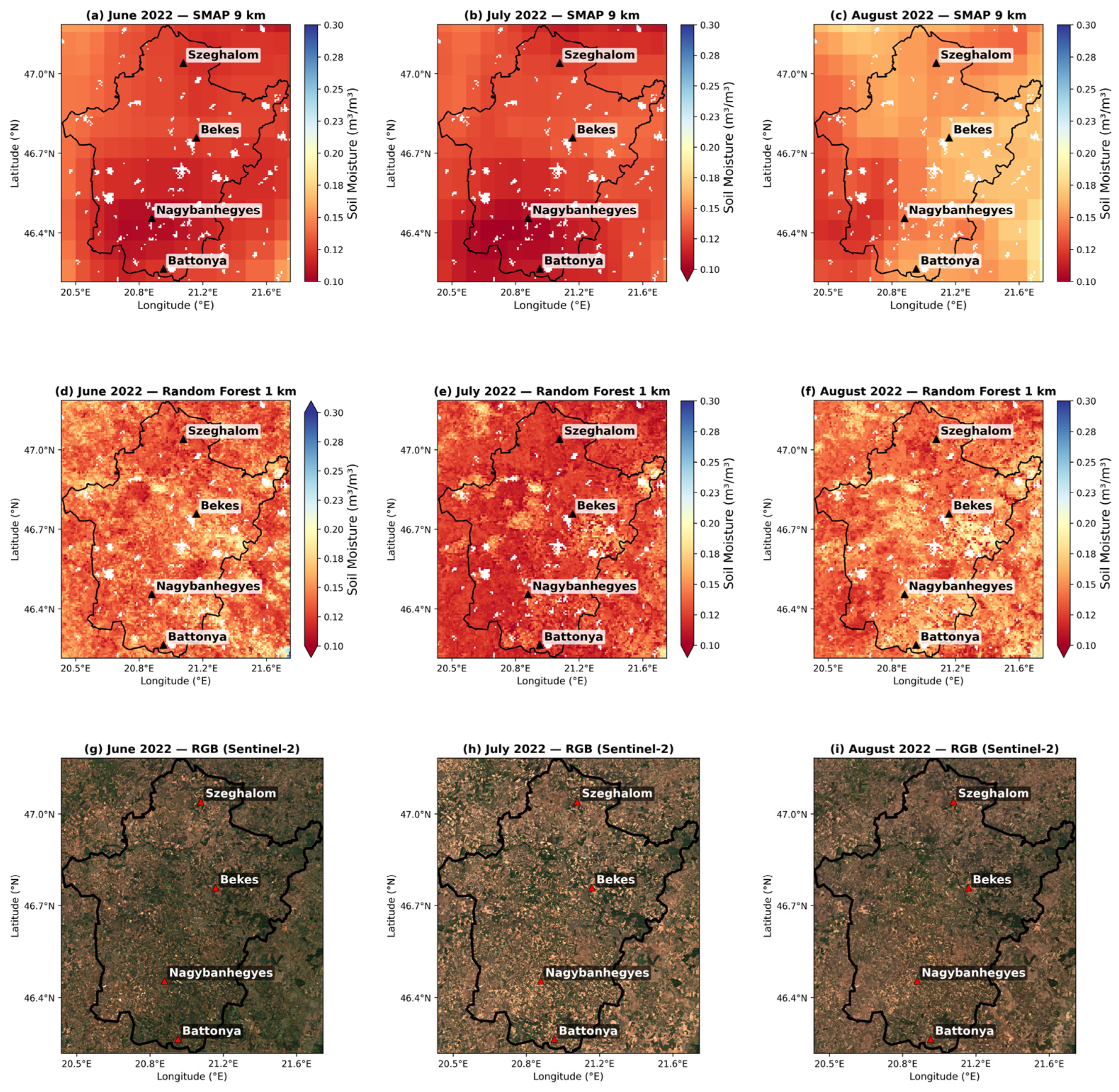
Figure 6 compares the mean monthly downscaled SM at 1 km resolution with the original SMAP product. Both datasets showed a drying trend from June to August, and the RF model accurately captured seasonal changes across all three months. Both products showed similar SM distributions, with drier areas in the south near Battonya and wetter areas in the north toward Szeghalom. These finer-detail maps help to capture local changes in soil moisture, driven by differences in land cover and topography across the Békés area. This improvement in spatial detail showed the RF model’s ability to generate physically consistent SM at a finer resolution while keeping the accuracy of the original satellite product.
Figure 6.
Comparison of spatial distribution of monthly mean SM (m3/m3) for June, July, and August 2022. Top row: SMAP 9 km original product, Middle row: Random Forest downscaled product at 1 km resolution, Bottom row: Sentinel-2 true-color RGB composite. Triangles represent in situ monitoring stations.
3.5. In Situ Validation
The validation of the RF downscale SM product against in situ data at four OVF stations is summarized in Table 5. Overall, across three stations, the 1 km RF model showed improved performance relative to the original 9 km SMAP. At Battonya, RF achieved a slight improvement in both R (0.609 vs. 0.591) and RMSE (0.058 vs. 0.065 m3 m−3), while Nagybánhegyes showed the most notable gain, with R increasing from 0.419 to 0.520 and RMSE decreasing from 0.096 to 0.085 m3 m−3. At Békés, improvements were marginal in R (0.380 vs. 0.375) and in RMSE (0.078 vs. 0.072 m3 m−3). Szeghalom was the only station where RF performed below SMAP in both metrics (R 0.452 vs. 0.585; RMSE 0.090 vs. 0.080 m3 m−3), which may reflect local spatial heterogeneity not fully captured at 1 km resolution. The validation process has two main limitations. First, the comparison uses a pixel-to-point approach, in which a 1 km model estimate is compared to a single in situ sensor that may not represent the entire pixel area. Second, the SMAP sensing depth (0–5 cm) does not match the in situ measurement depth (10 cm). This difference causes systematic changes in soil moisture dynamics across both products and likely reduces agreement with surface-based retrievals, regardless of model performance. Both products showed a consistent negative bias at every station, indicating that the observed underestimation is systematic. The corresponding unbiased RMSE (ubRMSE) values (0.0285–0.053 m3 m−3) are in the acceptable range of reported SMAP based products. To address the systematic bias, we applied a simple additive bias correction at each station, and the RMSE dropped by 40 to 55%.
Table 5.
Validation of SMAP 9 km and RF-downscaled 1 km SM at four stations.
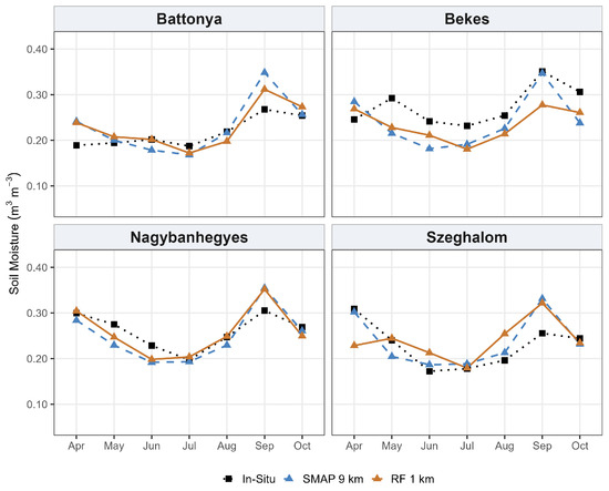
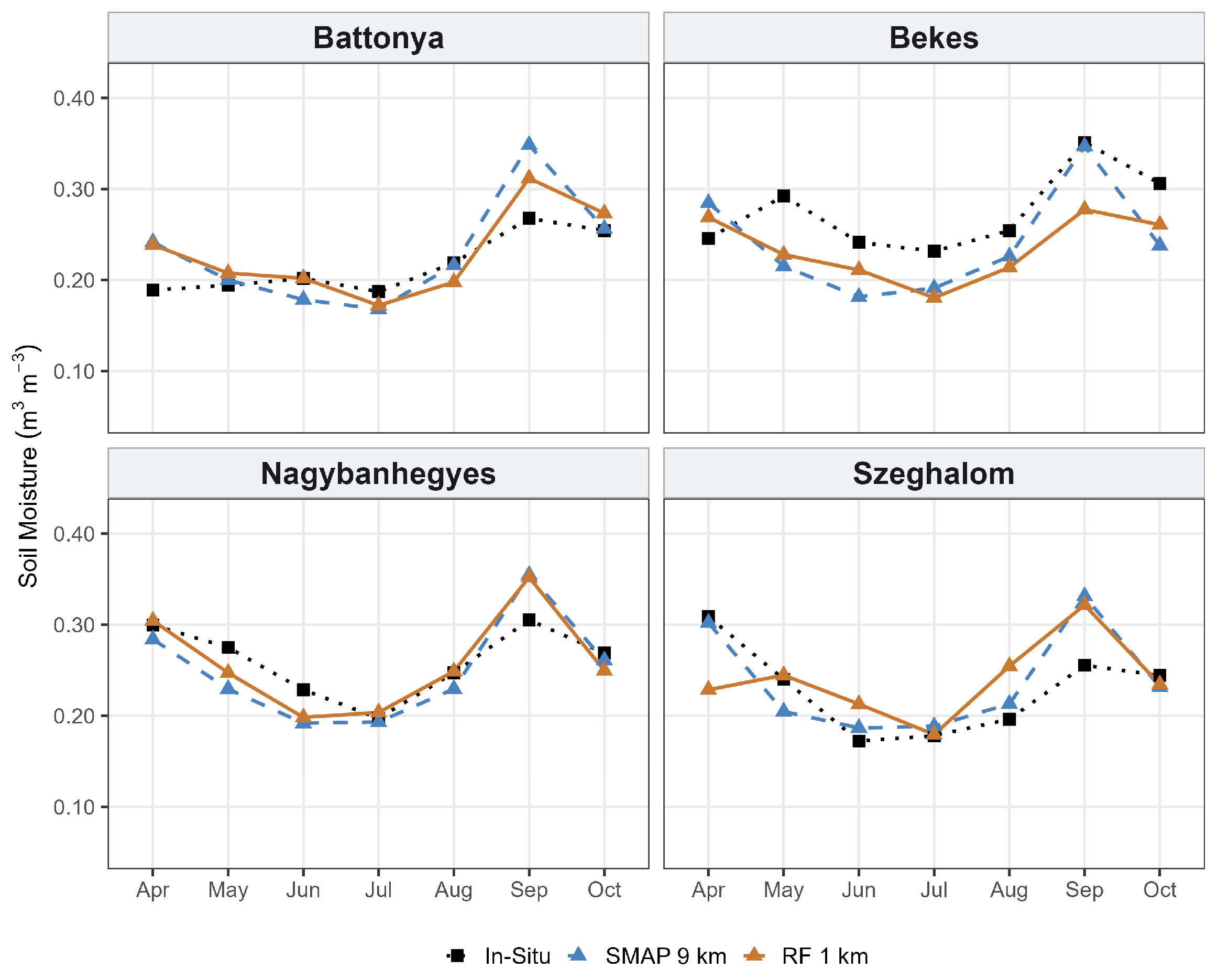
Figure 7 presents the bias-corrected monthly SM time series at the four validation stations for the 2022 growing season. After correction, both SMAP 9 km and RF 1 km showed similar seasonal cycles at most stations and months. At Battonya station, both products stayed within the same range (approximately 0.02 m3 m−3), but only in September did they overestimate the peak. Nagybanhegyes follows the same pattern with close agreement throughout the season (ranging from 0.19 to 0.36 m3 m−3), while the main deviation again occurs at the September peak, where both products overestimated by roughly 0.05 m3 m−3. In Békés, both products were consistently below the in situ graph, and in September, RF underestimated the September peak by 0.28 m3 m−3, while in situ reached its seasonal maximum of 0.351 m3 m−3. At the Szeghalom station, agreement was inconsistent across the season, and the error direction changed each month. RF underestimated in April, overestimated in August, and both products overestimated the September peak by 0.066–0.076 m3 m−3. This station is located in the Berettyó–Körös floodplain system at a low elevation (approximately 82 m) where a shallow groundwater table sustains near-surface SM through capillary rise. This makes it independent of surface conditions [81].
Figure 7.
Comparison of SMAP 9 km, RF-downscaled 1 km, and in situ soil moisture across the four OVF stations from April to October 2022.
3.6. Agricultural Drought Indices
In the final stage, the optimally trained RF model was applied to the complete time series of MODIS-derived predictors from 2004 to 2023 to generate spatially continuous SM maps at 1 km resolution across the study area. The original SMAP product is only available from 2015, which restricts the SSI baseline. However, because the trained RF model is independent of SMAP and relies solely on the auxiliary predictors used in this study, the SSI baseline for the 1 km downscaled SM data can be extended to 20 years.
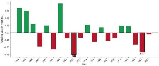
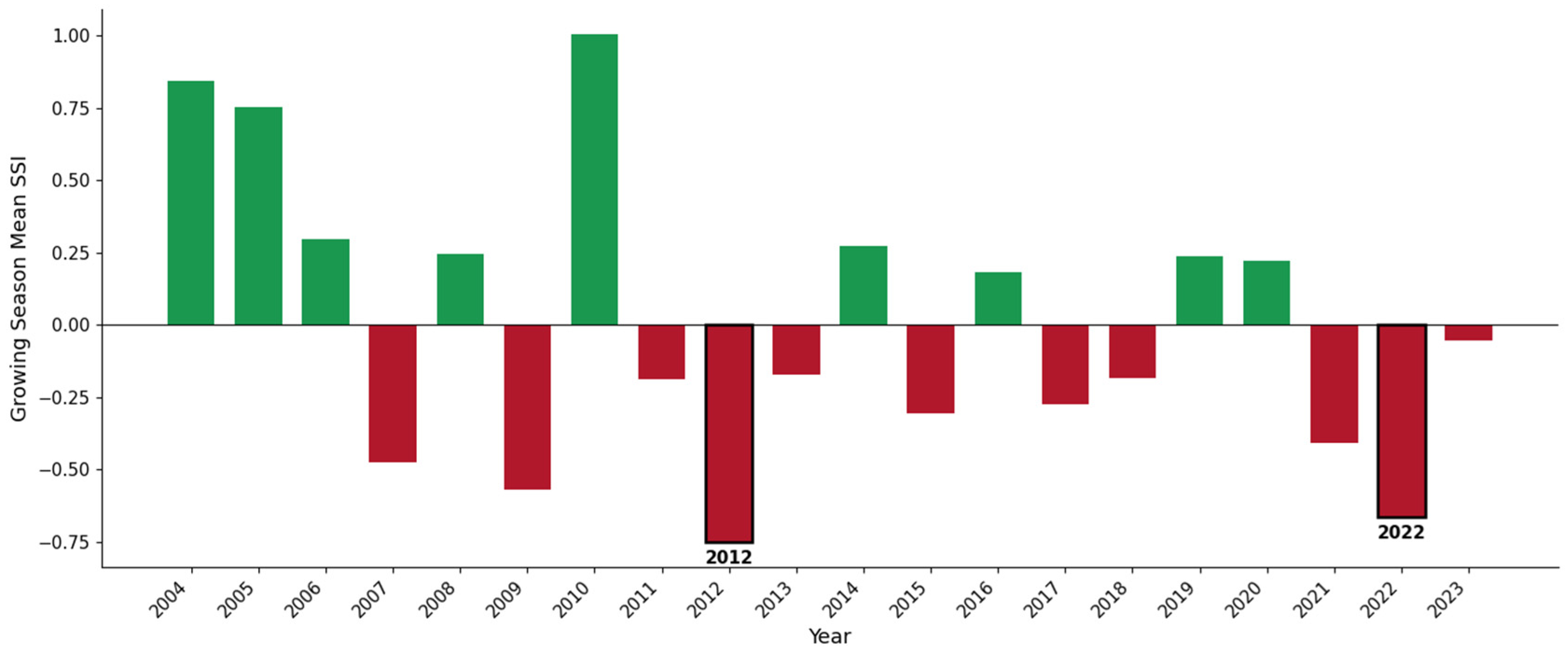
Figure 8 shows the bar chart of the 20-year growing-season mean SSI from 2004 to 2023. The record shows significant interannual variability. The two driest growing seasons were 2012 (mean SSI = −0.75) and 2022 (mean SSI = −0.66), consistent with historically documented severe drought events in Hungary [82,83]. In contrast, years including 2004, 2005, and 2010 showed wet conditions (mean SSI > 0.75), covering the full range of wet and dry conditions in the downscaled SSI product.
Figure 8.
Growing season mean Standardized Soil Moisture Index (SSI) by year (2004 to 2023). Green bars represent normal SM (positive SSI) and red bars represent below-normal SSI (negative SSI).
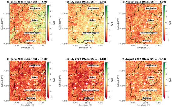
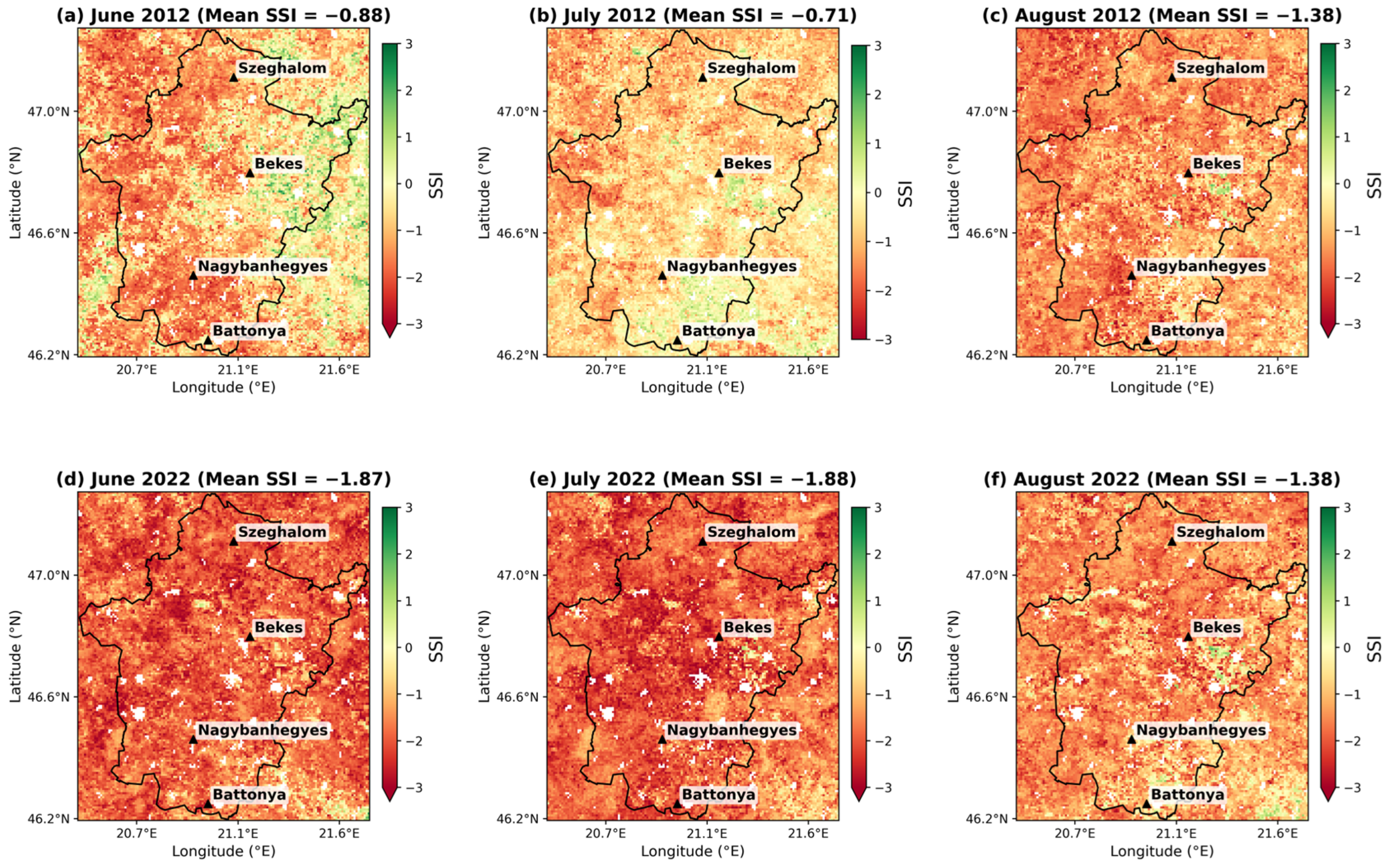
The SSI distribution of peak months from June to August is presented in Figure 9 for the years 2012 and 2022. In 2012, drought severity intensified progressively during summer, from a mean SSI = −0.88 in June to −1.38 in August. In 2022, drought conditions started earlier and became severe by June (SSI = −1.87), remaining severe in July (SSI = −1.88) and August (SSI = −1.38), reflecting the rapid onset of the 2022 drought. The contrast between the gradually intensifying drought in 2012 and the abrupt, sustained extreme event in 2022 is consistent with independent reports of the 2022 drought. These sources describe the 2022 event as exceptionally severe and rapid in onset, driven by extremely low precipitation and record summer temperatures across the Great Hungarian Plain.
Figure 9.
Monthly spatial distribution of SSI for June, July, and August of 2012 and 2022.
4. Discussion
4.1. Model Performance and Comparison
In this study, the RF model performed best among the tested algorithms, consistent with previous SMAP downscaling studies that report RF as a reliable and accurate algorithm for capturing nonlinear relationships between SM and land surface variables [45,68]. This advantage persisted following hyperparameter tuning for each model. RF achieved its best performance (R2 = 0.711) with a relatively simple configuration: 100 trees and unrestricted depth. In contrast, XGBoost required substantially more boosting iterations (5000 estimators) and a lower learning rate (0.05) to attain comparable accuracy (R2 = 0.694). GBM’s best configuration (500 estimators, learning rate = 0.05, max depth = 5) achieved only R2 = 0.507, the largest performance gap among the three models. In a multimodal fusion study, the RF model achieved a high accuracy of R2 = 0.92, significantly outperforming XGBoost (R2 = 0.76) [68]. In another study conducted in the Shandian River (SDR) Basin, researchers compared RF and XGB (XGBoost) for downscaling to 1 km and 100 m resolutions. In this specific region, RF outperformed XGBoost at both scales: at 1 km, RF achieved an R2 of 0.77 compared to XGBoost’s 0.605 [33]. RF outperformed XGBoost and GBM because it creates multiple independent decision trees from random subsets of the data and then averages their results [79]. This approach helps reduce the impact of noise in satellite-derived inputs. In contrast, XGBoost and GBM build trees sequentially, with each new tree trying to correct the previous one’s mistakes [35]. This process makes them more sensitive to noisy or irregular data, a pattern our tuning results support directly, since GBM’s accuracy plateaued well below RF’s even with additional trees and careful learning-rate adjustment.
4.2. Predictors Importance
To assess the role of each predictor, feature importance analysis was conducted. The result showed that daytime LST was the dominant variable across all three models, followed by ET and nighttime LST, whereas NDVI and land cover type contributed the least to SM estimation. This finding is consistent with previous studies that identified LST as a key predictor in machine-learning SM downscaling methods [24,33,36,84]. LST is directly connected to SM—wet soils stay cooler because water evaporates, carrying heat away, while dry soils heat up quickly due to limited evaporation [52,85]. The superiority of daytime over nighttime LST reflects the stronger thermal response to solar radiation during the daytime, whereas nighttime surface conditions tend toward thermal equilibrium, reducing the sensitivity of nocturnal LST to SM [52]. ET ranked second in RF and GBM, directly reflecting SM availability through plant transpiration and surface evaporation [86]. Under drought conditions, both transpiration and evaporation decline as SM becomes limited, and ET decreases accordingly [86]. EVI consistently outperformed NDVI, likely due to its lower sensitivity to saturation in the densely vegetated cropland landscape of Békés County [87].
4.3. Systematic Bias Correction and Site-Specific Model Performance
The systematic underestimation of SM observed at the validation stations showed the physical principle of L-band passive microwave retrieval rather than a model deficiency [37]. SMAP measures emitted microwave radiation governed by soil’s dielectric constant. However, this signal penetrates only to the top 5 cm of the soil column [88]. The top centimeters of soil dry faster due to solar radiation and evaporative demand, while the 10 cm layer retains more water due to gravitational infiltration. Although a systematic offset was observed, the range of ubRMSE values in this study was from 0.029 to 0.053 m3 m−3, which aligns with the NASA SMAP mission’s accuracy target of ubRMSE less than 0.04 m3 m−3 [86]. Specifically, Battonya, Békés, and Nagybanhegyes either meet or closely approach this threshold. These findings suggest that, after accounting for the systematic depth-related bias, the random error component of both products remains within the range deemed reliable for hydrological and agricultural applications. Szeghalom is located in the Berettyó–Körös floodplain system at a low elevation where a shallow groundwater table sustains near-surface SM through capillary rise, making it largely independent of surface conditions [81]. Because the RF downscaling model is trained on surface predictors—vegetation indices, land surface temperature, and terrain attributes—that assume soil moisture variability is driven primarily by surface energy and vegetation fluxes, this assumption breaks down at Szeghalom. As a result, the relationships learned across the rest of the study domain transfer poorly to this station, degrading RF’s performance below that of the native SMAP retrieval, which is comparatively less sensitive to this kind of fine-scale surface heterogeneity.
4.4. Application for Agricultural Drought Monitoring
Downscaled SSI maps indicate that July 2022 experienced the most severe drought in Békés County. This finding aligns with other regional evidence confirming that 2022 was the worst drought on the Great Hungarian Plain since 1975 [89]. The consistent occurrence of extreme negative SSI values across all four monitoring stations and throughout the county highlights the diagnostic utility of the 1 km downscaled product for county-scale agricultural drought monitoring. This approach enables the identification of spatial patterns of drought severity that are not discernible at the original 9 km SMAP resolution.
4.5. Limitations and Future Work
This study has several limitations. As the approach relies on optical and thermal MODIS data, cloud cover can occasionally restrict data availability. Integrating Sentinel-1 Synthetic Aperture Radar (SAR) data in future studies could help overcome this limitation. Furthermore, higher-resolution soil and irrigation data integration as supplementary inputs could improve local accuracy in agricultural regions. The monthly temporal resolution used to compute the SSI, while suitable for capturing seasonal and inter-annual drought patterns, does not capture short-term soil moisture dynamics such as rapid wetting after rainfall and subsequent drying [45]. Future research will prioritize (1) incorporating additional independently derived high-resolution soil moisture products, such as Sentinel-1 SAR retrievals, to decrease reliance on a single satellite source; (2) extending the temporal resolution of the framework to better capture short-term soil moisture dynamics relevant to rapid-onset agricultural drought; and (3) expanding the in situ validation network to more comprehensively characterize model performance across the full spectrum of local soil and land management conditions in the region.
5. Conclusions
This study developed a framework to downscale SMAP soil moisture data from 9 to 1 km using machine learning algorithms over Békés County, Hungary, during the growing seasons of 2020–2023. Multi-source auxiliary fine-resolution variables, such as MODIS vegetation, thermal, and evapotranspiration data, along with land cover and elevation, were used to enhance the resolution of the SMAP 9 km product to 1 km. This study focused on the agricultural landscape and used fine-resolution results to produce an SSI drought index maps for practical agricultural monitoring.
Among the three ML models tested, RF was selected as the optimal downscaling approach due to its higher accuracy. Daytime LST was the most influential predictor across all models, reflecting the strong link between thermal and moisture dynamics in agricultural landscapes. Validation at four in situ stations showed that the RF-downscaled product generally outperformed the original SMAP 9 km retrievals. The resulting 1 km SSI maps revealed inter-annual drought variability that was not visible at coarser resolutions and identified July 2022 as the most severe drought during the study period.
Supplementary Materials
The following supporting information can be downloaded at https://www.mdpi.com/article/10.3390/agriengineering8090373/s1: Table S1: Hyperparameter configurations for Random Forest, XGBoost, and Gradient Boosting Machine (GBM) models; Figure S1: Spatial distribution of monthly mean soil moisture (m3/m3) for all growing season months (April–October) 2022; Figure S2: Spatial distribution of July soil moisture (m3/m3) for all study years (2020–2023); Figure S3: Scatterplot of Predicted vs. In situ SM.
Author Contributions
Conceptualization, M.S. and I.W.; methodology, M.S.; software, M.S.; validation, M.S. and G.E.H.; formal analysis, M.S.; investigation, M.S.; resources, Z.V.; data curation, M.S.; writing—original draft preparation, M.S.; writing—review and editing, I.W., Z.V., and G.E.H.; visualization, M.S.; project administration, I.W.; supervision, I.W. and Z.V. All authors have read and agreed to the published version of the manuscript.
Funding
This research received no external funding.
Institutional Review Board Statement
Not applicable.
Informed Consent Statement
Not applicable.
Data Availability Statement
The data that support the findings of this study are available from the corresponding author upon reasonable request.
Acknowledgments
The author (M.S.) is also grateful to the Hungarian Tempus Public Foundation for the Stipendium Hungaricum scholarship.
Conflicts of Interest
The authors declare no conflicts of interest.
Abbreviations
The following abbreviations are used in this manuscript:
| DEM | Digital Elevation Model |
| ET | Evapotranspiration |
| EVI | Enhanced Vegetation Index |
| GBM | Gradient Boosting Machine |
| GEE | Google Earth Engine |
| LC | Land Cover |
| LST | Land Surface Temperature |
| MAE | Mean Absolute Error |
| MDI | Mean Decrease in Impurity |
| ML | Machine Learning |
| MODIS | Moderate Resolution Imaging Spectroradiometer |
| NDVI | Normalized Difference Vegetation Index |
| OVF | Országos Vízügyi Főigazgatóság (Hungarian National Water Directorate) |
| RF | Random Forest |
| RMSE | Root Mean Square Error |
| RS | Remote Sensing |
| SAR | Synthetic Aperture Radar |
| SDR | ShanDian River |
| SM | Soil Moisture |
| SMAP | Soil Moisture Active Passive |
| SSI | Standardized Soil Moisture Index |
| ubRMSE | Unbiased Root Mean Square Error |
| USGS | U.S. Geological Survey |
| XGBoost | Extreme Gradient Boosting |
References
- Peng, J.; Loew, A.; Merlin, O.; Verhoest, N.E.C. A Review of Spatial Downscaling of Satellite Remotely Sensed Soil Moisture. Rev. Geophys. 2017, 55, 341–366. [Google Scholar] [CrossRef] [Scilit]
- Mallik, S.; Chakraborty, A.; Podder, K.; Talukdar, S.; Rahman, A.; Mishra, U. Enhancing Soil Moisture Prediction with Explainable AI: Integrating IoT and Multi-Sensor Remote Sensing Data through Soft Computing. Appl. Soft Comput. 2025, 180, 113406. [Google Scholar] [CrossRef] [Scilit]
- Kuang, X.; Xiang, S.; Guo, J. Soil Moisture Retrieval and Trend Prediction Using Multi-Temporal Remote Sensing Data: An Interpretable Deep Regression Approach. Expert Syst. Appl. 2025, 287, 128172. [Google Scholar] [CrossRef] [Scilit]
- Seneviratne, S.; Nicholls, N.; Easterling, D.; Goodess, C.; Kanae, S.; Kossin, J.; Luo, Y.; Marengo, J.; McInnes, K.; Rahimi, M.; et al. Changes in Climate Extremes and Their Impacts on the Natural Physical Environment. In Managing the Risks of Extreme Events and Disasters to Advance Climate Change Adaptation; Cambridge University Press: Cambridge, UK; New York, NY, USA, 2012; pp. 109–230. [Google Scholar] [CrossRef]
- Hanel, M.; Rakovec, O.; Markonis, Y.; Máca, P.; Samaniego, L.; Kyselý, J.; Kumar, R. Revisiting the Recent European Droughts from a Long-Term Perspective. Sci. Rep. 2018, 8, 9499. [Google Scholar] [CrossRef] [Scilit] [PubMed]
- Mezősi, G.; Bata, T.; Meyer, B.C.; Blanka, V.; Ladányi, Z. Climate Change Impacts on Environmental Hazards on the Great Hungarian Plain, Carpathian Basin. Int. J. Disaster Risk Sci. 2014, 5, 136–146. [Google Scholar] [CrossRef] [Scilit][Green Version]
- Jia, A.; Mallick, K.; Upadhyaya, D.; Hu, T.; Szantoi, Z.; Bhattacharya, B.; Sekhar, M.; Skoković, D.; Sobrino, J.A.; Ruiz, L.; et al. Deriving a Clear-Sky Soil Moisture Index from ECOSTRESS Land Surface Temperature. Remote Sens. Environ. 2025, 329, 114945. [Google Scholar] [CrossRef] [Scilit]
- Adab, H.; Morbidelli, R.; Saltalippi, C.; Moradian, M.; Ghalhari, G.A.F. Machine Learning to Estimate Surface Soil Moisture from Remote Sensing Data. Water 2020, 12, 3223. [Google Scholar] [CrossRef] [Scilit]
- Abbes, A.B.; Jarray, N.; Farah, I.R. Advances in Remote Sensing Based Soil Moisture Retrieval: Applications, Techniques, Scales and Challenges for Combining Machine Learning and Physical Models. Artif. Intell. Rev. 2024, 57, 224. [Google Scholar] [CrossRef] [Scilit]
- Schmugge, T.J.; Jackson, T.J.; McKim, H.L. Survey of Methods for Soil Moisture Determination. Water Resour. Res. 1980, 16, 961–979. [Google Scholar] [CrossRef] [Scilit]
- Collow, T.W.; Robock, A.; Basara, J.B.; Illston, B.G. Evaluation of SMOS Retrievals of Soil Moisture over the Central United States with Currently Available in Situ Observations. J. Geophys. Res. Atmos. 2012, 117, D09113. [Google Scholar] [CrossRef] [Scilit]
- Mukhlisin, M.; Astuti, H.W.; Wardihani, E.D.; Matlan, S.J. Techniques for Ground-Based Soil Moisture Measurement: A Detailed Overview. Arab. J. Geosci. 2021, 14, 2032. [Google Scholar] [CrossRef] [Scilit]
- Dari, J.; Quintana-Seguí, P.; Escorihuela, M.J.; Stefan, V.; Brocca, L.; Morbidelli, R. Detecting and Mapping Irrigated Areas in a Mediterranean Environment by Using Remote Sensing Soil Moisture and a Land Surface Model. J. Hydrol. 2021, 596, 126129. [Google Scholar] [CrossRef] [Scilit]
- Cheng, M.; Li, B.; Jiao, X.; Huang, X.; Fan, H.; Lin, R.; Liu, K. Using Multimodal Remote Sensing Data to Estimate Regional-Scale Soil Moisture Content: A Case Study of Beijing, China. Agric. Water Manag. 2022, 260, 107298. [Google Scholar] [CrossRef] [Scilit]
- Monteiro, A.T.; Arenas-Castro, S.; Punalekar, S.M.; Cunha, M.; Mendes, I.; Giamberini, M.; Marques da Costa, E.; Fava, F.; Lucas, R. Remote Sensing of Vegetation and Soil Moisture Content in Atlantic Humid Mountains with Sentinel-1 and 2 Satellite Sensor Data. Ecol. Indic. 2024, 163, 112123. [Google Scholar] [CrossRef] [Scilit]
- Liu, Y.; Jing, W.; Wang, Q.; Xia, X. Generating High-Resolution Daily Soil Moisture by Using Spatial Downscaling Techniques: A Comparison of Six Machine Learning Algorithms. Adv. Water Resour. 2020, 141, 103601. [Google Scholar] [CrossRef] [Scilit]
- Santi, E.; Paloscia, S.; Pettinato, S.; Brocca, L.; Ciabatta, L.; Entekhabi, D. On the Synergy of SMAP, AMSR2 AND SENTINEL-1 for Retrieving Soil Moisture. Int. J. Appl. Earth Obs. Geoinf. 2018, 65, 114–123. [Google Scholar] [CrossRef] [Scilit]
- Mao, H.; Kathuria, D.; Duffield, N.; Mohanty, B.P. Gap Filling of High-Resolution Soil Moisture for SMAP/Sentinel-1: A Two-Layer Machine Learning-Based Framework. Water Resour. Res. 2019, 55, 6986–7009. [Google Scholar] [CrossRef] [Scilit]
- Reddy, G.P.O. Satellite Remote Sensing Sensors: Principles and Applications. In Geospatial Technologies in Land Resources Mapping, Monitoring and Management; Reddy, G.P.O., Singh, S.K., Eds.; Springer International Publishing: Cham, Switzerland, 2018; pp. 21–43. ISBN 978-3-319-78711-4. [Google Scholar]
- Entekhabi, D.; Njoku, E.G.; O’Neill, P.E.; Kellogg, K.H.; Crow, W.T.; Edelstein, W.N.; Entin, J.K.; Goodman, S.D.; Jackson, T.J.; Johnson, J.; et al. The Soil Moisture Active Passive (SMAP) Mission. Proc. IEEE 2010, 98, 704–716. [Google Scholar] [CrossRef] [Scilit]
- Entekhabi, D.; Njoku, E.; O’Neill, P.; Kellogg, K.; Entin, J. The NASA Soil Moisture Active Passive (SMAP) Mission Formulation. In Proceedings of the 2011 IEEE International Geoscience and Remote Sensing Symposium, Vancouver, BC, Canada, 24–29 July 2011; pp. 2302–2305. [Google Scholar]
- Vergopolan, N.; Sheffield, J.; Chaney, N.W.; Pan, M.; Beck, H.E.; Ferguson, C.R.; Torres-Rojas, L.; Eigenbrod, F.; Crow, W.; Wood, E.F. High-Resolution Soil Moisture Data Reveal Complex Multi-Scale Spatial Variability Across the United States. Geophys. Res. Lett. 2022, 49, e2022GL098586. [Google Scholar] [CrossRef] [Scilit]
- Fang, B.; Lakshmi, V.; Bindlish, R.; Jackson, T.J. Downscaling of SMAP Soil Moisture Using Land Surface Temperature and Vegetation Data. Vadose Zone J. 2018, 17, 170198. [Google Scholar] [CrossRef] [Scilit]
- Zhao, W.; Sánchez, N.; Lu, H.; Li, A. A Spatial Downscaling Approach for the SMAP Passive Surface Soil Moisture Product Using Random Forest Regression. J. Hydrol. 2018, 563, 1009–1024. [Google Scholar] [CrossRef] [Scilit]
- Van der Schalie, R.; De Jeu, R.; Parinussa, R.; Rodríguez-Fernández, N.; Kerr, Y.; Al-Yaari, A.; Wigneron, J.-P.; Drusch, M. The Effect of Three Different Data Fusion Approaches on the Quality of Soil Moisture Retrievals from Multiple Passive Microwave Sensors. Remote Sens. 2018, 10, 107. [Google Scholar] [CrossRef] [Scilit]
- Arab, S.; Easson, G.; Ghaffari, Z. Integration of Sentinel-1A Radar and SMAP Radiometer for Soil Moisture Retrieval over Vegetated Areas. Sensors 2024, 24, 2217. [Google Scholar] [CrossRef] [Scilit] [PubMed]
- Ma, H.; Zeng, J.; Zhang, X.; Peng, J.; Li, X.; Fu, P.; Cosh, M.H.; Letu, H.; Wang, S.; Chen, N.; et al. Surface Soil Moisture from Combined Active and Passive Microwave Observations: Integrating ASCAT and SMAP Observations Based on Machine Learning Approaches. Remote Sens. Environ. 2024, 308, 114197. [Google Scholar] [CrossRef] [Scilit]
- Chen, S.; She, D.; Zhang, L.; Guo, M.; Liu, X. Spatial Downscaling Methods of Soil Moisture Based on Multisource Remote Sensing Data and Its Application. Water 2019, 11, 1401. [Google Scholar] [CrossRef] [Scilit]
- Abbaszadeh, P.; Moradkhani, H.; Gavahi, K.; Kumar, S.; Hain, C.; Zhan, X.; Duan, Q.; Peters-Lidard, C.; Karimiziarani, S. High-Resolution SMAP Satellite Soil Moisture Product: Exploring the Opportunities. Bull. Am. Meteorol. Soc. 2021, 102, 309–315. [Google Scholar] [CrossRef] [Scilit]
- Bai, L.; Long, D.; Yan, L. Estimation of Surface Soil Moisture With Downscaled Land Surface Temperatures Using a Data Fusion Approach for Heterogeneous Agricultural Land. Water Resour. Res. 2019, 55, 1105–1128. [Google Scholar] [CrossRef] [Scilit]
- Zhao, Z.; Jin, R.; Kang, J.; Ma, C.; Wang, W. Using of Remote Sensing-Based Auxiliary Variables for Soil Moisture Scaling and Mapping. Remote Sens. 2022, 14, 3373. [Google Scholar] [CrossRef] [Scilit]
- Sishah, S.; Abrahem, T.; Azene, G.; Dessalew, A.; Hundera, H. Downscaling and Validating SMAP Soil Moisture Using a Machine Learning Algorithm over the Awash River Basin, Ethiopia. PLoS ONE 2023, 18, e0279895. [Google Scholar] [CrossRef] [Scilit] [PubMed]
- Wang, J.; Xue, H.; Dong, G.; Yuan, Q.; Zhang, R.; Jing, R. Downscaling of Remote Sensing Soil Moisture Products That Integrate Microwave and Optical Data. Appl. Sci. 2024, 14, 11875. [Google Scholar] [CrossRef] [Scilit]
- Molero, B.; Merlin, O.; Malbéteau, Y.; Al Bitar, A.; Cabot, F.; Stefan, V.; Kerr, Y.; Bacon, S.; Cosh, M.H.; Bindlish, R.; et al. SMOS Disaggregated Soil Moisture Product at 1 Km Resolution: Processor Overview and First Validation Results. Remote Sens. Environ. 2016, 180, 361–376. [Google Scholar] [CrossRef] [Scilit]
- Teixeira, A.C.; Bakon, M.; Lopes, D.; Cunha, A.; Sousa, J.J. A Systematic Review on Soil Moisture Estimation Using Remote Sensing Data for Agricultural Applications. Sci. Remote Sens. 2025, 12, 100328. [Google Scholar] [CrossRef] [Scilit]
- Poehls, J.; Alonso, L.; Koirala, S.; Reichstein, M.; Carvalhais, N. Downscaling Soil Moisture to Sub-Km Resolutions with Simple Machine Learning Ensembles. J. Hydrol. 2025, 652, 132624. [Google Scholar] [CrossRef] [Scilit]
- Xu, J.; Su, Q.; Li, X.; Ma, J.; Song, W.; Zhang, L.; Su, X. A Spatial Downscaling Framework for SMAP Soil Moisture Based on Stacking Strategy. Remote Sens. 2024, 16, 200. [Google Scholar] [CrossRef] [Scilit]
- Fang, B.; Lakshmi, V.; Cosh, M.; Liu, P.-W.; Bindlish, R.; Jackson, T.J. A Global 1-Km Downscaled SMAP Soil Moisture Product Based on Thermal Inertia Theory. Vadose Zone J. 2022, 21, e20182. [Google Scholar] [CrossRef] [Scilit]
- Jin, Y.; Ge, Y.; Liu, Y.; Chen, Y.; Zhang, H.; Heuvelink, G.B.M. A Machine Learning-Based Geostatistical Downscaling Method for Coarse-Resolution Soil Moisture Products. IEEE J. Sel. Top. Appl. Earth Obs. Remote Sens. 2021, 14, 1025–1037. [Google Scholar] [CrossRef] [Scilit]
- Im, J.; Park, S.; Rhee, J.; Baik, J.; Choi, M. Downscaling of AMSR-E Soil Moisture with MODIS Products Using Machine Learning Approaches. Environ. Earth Sci. 2016, 75, 1120. [Google Scholar] [CrossRef] [Scilit]
- Liu, Y.; Qian, J.; Yue, H. Combined Sentinel-1A With Sentinel-2A to Estimate Soil Moisture in Farmland. IEEE J. Sel. Top. Appl. Earth Obs. Remote Sens. 2021, 14, 1292–1310. [Google Scholar] [CrossRef] [Scilit]
- Zheng, M.; Liu, Z.; Li, J.; Xu, Z.; Sun, J. Downscaling Soil Moisture in Regions with High Soil Heterogeneity: The Solution Based on Ensemble Learning with Sequential and Parallel Learner. Sci. Total Environ. 2024, 950, 175260. [Google Scholar] [CrossRef] [Scilit] [PubMed]
- Srivastava, P.K.; Han, D.; Ramirez, M.R.; Islam, T. Machine Learning Techniques for Downscaling SMOS Satellite Soil Moisture Using MODIS Land Surface Temperature for Hydrological Application. Water Resour. Manag. 2013, 27, 3127–3144. [Google Scholar] [CrossRef] [Scilit]
- Zhang, Y.; Chen, Y.; Chen, L.; Xu, S.; Sun, H. A Machine Learning-Based Approach for Generating High-Resolution Soil Moisture from SMAP Products. Geocarto Int. 2022, 37, 16086–16107. [Google Scholar] [CrossRef] [Scilit]
- Wang, Y.; Shi, H.; Yang, X.; Jiang, Y.; Wu, Y.; Shui, J.; Liu, Y.; Guo, M.; Li, L. Spatial Downscaling of SMAP Soil Moisture to High Resolution Using Machine Learning over China’s Loess Plateau. CATENA 2024, 247, 108492. [Google Scholar] [CrossRef] [Scilit]
- Wei, Z.; Meng, Y.; Zhang, W.; Peng, J.; Meng, L. Downscaling SMAP Soil Moisture Estimation with Gradient Boosting Decision Tree Regression over the Tibetan Plateau. Remote Sens. Environ. 2019, 225, 30–44. [Google Scholar] [CrossRef] [Scilit]
- Fang, B.; Kansara, P.; Dandridge, C.; Lakshmi, V. Drought Monitoring Using High Spatial Resolution Soil Moisture Data over Australia in 2015–2019. J. Hydrol. 2021, 594, 125960. [Google Scholar] [CrossRef] [Scilit]
- Bolten, J.D.; Crow, W.T.; Zhan, X.; Jackson, T.J.; Reynolds, C.A. Evaluating the Utility of Remotely Sensed Soil Moisture Retrievals for Operational Agricultural Drought Monitoring. IEEE J. Sel. Top. Appl. Earth Obs. Remote Sens. 2010, 3, 57–66. [Google Scholar] [CrossRef] [Scilit]
- Hao, Z.; AghaKouchak, A. Multivariate Standardized Drought Index: A Parametric Multi-Index Model. Adv. Water Resour. 2013, 57, 12–18. [Google Scholar] [CrossRef] [Scilit]
- Trnka, M.; Hlavinka, P.; Možný, M.; Semerádová, D.; Štěpánek, P.; Balek, J.; Bartošová, L.; Zahradníček, P.; Bláhová, M.; Skalák, P.; et al. Czech Drought Monitor System for Monitoring and Forecasting Agricultural Drought and Drought Impacts. Int. J. Climatol. 2020, 40, 5941–5958. [Google Scholar] [CrossRef] [Scilit]
- Kumhálová, J.; Sedlák, J.; Marčan, J.; Vandírková, V.; Novotný, P.; Kohútek, M.; Kumhála, F. Monitoring of Agricultural Crops by Remote Sensing in Central Europe: A Comprehensive Review. Remote Sens. 2026, 18, 1075. [Google Scholar] [CrossRef] [Scilit]
- Pablos, M.; Martínez-Fernández, J.; Sánchez, N.; González-Zamora, Á. Temporal and Spatial Comparison of Agricultural Drought Indices from Moderate Resolution Satellite Soil Moisture Data over Northwest Spain. Remote Sens. 2017, 9, 1168. [Google Scholar] [CrossRef] [Scilit]
- Ning, J.; Yao, Y.; Fisher, J.B.; Li, Y.; Zhang, X.; Jiang, B.; Xu, J.; Yu, R.; Liu, L.; Zhang, X.; et al. Soil Moisture-Derived SWDI at 30 m Based on Multiple Satellite Datasets for Agricultural Drought Monitoring. Remote Sens. 2024, 16, 3372. [Google Scholar] [CrossRef] [Scilit]
- Madelon, R.; Rodríguez-Fernández, N.J.; Bazzi, H.; Baghdadi, N.; Albergel, C.; Dorigo, W.; Zribi, M. Soil Moisture Estimates at 1 km Resolution Making a Synergistic Use of Sentinel Data. Hydrol. Earth Syst. Sci. 2023, 27, 1221–1242. [Google Scholar] [CrossRef] [Scilit]
- Pécsi, M. Geomorphological Regions in Hungary; Hungarian Academy of Sciences: Budapest, Hungary, 1996; ISBN 978-963-7395-74-1. [Google Scholar]
- Bolla, B.; Manninger, M.; Molnár, T.; Horváth, B.; Szolgay, J.; Gribovszki, Z.; Kalicz, P.; Szabó, A. Evaluation of the Compound Effects of the 2022 Drought and Heatwave on Selected Forest Monitoring Sites in Hungary in Relation to Its Multi-Year Drought Legacy. Forests 2024, 15, 941. [Google Scholar] [CrossRef] [Scilit]
- Blanka-Végi, V.; Tobak, Z.; Sipos, G.; Barta, K.; Szabó, B.; van Leeuwen, B. Estimation of the Spatiotemporal Variability of Surface Soil Moisture Using Machine Learning Methods Integrating Satellite and Ground-Based Soil Moisture and Environmental Data. Water Resour. Manag. 2025, 39, 2317–2334. [Google Scholar] [CrossRef] [Scilit]
- Fiala, K.; Harsányi, E.; Gaál, M.; Tarjáni, G. Operatív aszály-és vízhiánykezelő monitoring rendszer [Operational drought and water scarcity monitoring system]. Hidrol. Közlöny [J. Hung. Hydrol. Soc.] 2018, 98, 14–24. [Google Scholar]
- Placidi, P.; Gasperini, L.; Grassi, A.; Cecconi, M.; Scorzoni, A. Characterization of Low-Cost Capacitive Soil Moisture Sensors for IoT Networks. Sensors 2020, 20, 3585. [Google Scholar] [CrossRef] [Scilit] [PubMed]
- Didan, K. MODIS/Terra Vegetation Indices 16-Day L3 Global 500 m SIN Grid V061; NASA EOSDIS Land Processes Distributed Active Archive Center: Sioux Falls, SD, USA, 2021.
- Wan, Z.; Hook, S.; Hulley, G. MODIS/Terra Land Surface Temperature/Emissivity 8-Day L3 Global 1 km SIN Grid V061; NASA EOSDIS Land Processes Distributed Active Archive Center: Sioux Falls, SD, USA, 2021. [CrossRef]
- Running, S.; Mu, Q.; Zhao, M.; Moreno, A. MODIS/Terra Net Evapotranspiration Gap-Filled 8-Day L4 Global 500 m SIN Grid V061; NASA EOSDIS Land Processes Distributed Active Archive Center: Sioux Falls, SD, USA, 2021. [CrossRef]
- U.S. Geological Survey. Global 30 Arc-Second Elevation (GTOPO30); U.S. Geological Survey: Reston, VA, USA, 1996. [CrossRef] [Scilit]
- Friedl, M.; Sulla-Menashe, D. MODIS/Terra+Aqua Land Cover Type Yearly L3 Global 500 m SIN Grid V061; NASA EOSDIS Land Processes Distributed Active Archive Center: Sioux Falls, SD, USA, 2022. [CrossRef]
- O’Neill, P.; Chan, S.; Njoku, E.; Jackson, T.; Bindlish, R.; Chaubell, J.; Colliander, A. SMAP Enhanced L3 Radiometer Global and Polar Grid Daily 9 km EASE-Grid Soil Moisture, Version 5; NASA National Snow and Ice Data Center Distributed Active Archive Center: Sioux Falls, SD, USA, 2021. [CrossRef]
- Colliander, A.; Jackson, T.J.; Bindlish, R.; Chan, S.; Das, N.; Kim, S.B.; Cosh, M.H.; Dunbar, R.S.; Dang, L.; Pashaian, L.; et al. Validation of SMAP Surface Soil Moisture Products with Core Validation Sites. Remote Sens. Environ. 2017, 191, 215–231. [Google Scholar] [CrossRef] [Scilit]
- Breiman, L. Random Forests. Mach. Learn. 2001, 45, 5–32. [Google Scholar] [CrossRef] [Scilit]
- Sang, X.; Lu, X.; Wang, K.; Zhou, J.; Cai, G.; Fan, J. SMAP Soil Moisture Downscaling Via Multimodal Data Fusion and Machine Learning. Earth Syst. Environ. 2026, 10, 7833–7852. [Google Scholar] [CrossRef] [Scilit]
- He, X.; Chaney, N.W.; Schleiss, M.; Sheffield, J. Spatial Downscaling of Precipitation Using Adaptable Random Forests. Water Resour. Res. 2016, 52, 8217–8237. [Google Scholar] [CrossRef] [Scilit]
- Friedman, J.H. Greedy Function Approximation: A Gradient Boosting Machine. Ann. Stat. 2001, 29, 1189–1232. [Google Scholar] [CrossRef] [Scilit]
- Chen, T.; Guestrin, C. XGBoost: A Scalable Tree Boosting System. In Proceedings of the Proceedings of the 22nd ACM SIGKDD International Conference on Knowledge Discovery and Data Mining; Association for Computing Machinery: New York, NY, USA, 2016; pp. 785–794. [Google Scholar]
- Zhang, Y.; Liang, S.; Zhu, Z.; Ma, H.; He, T. Soil Moisture Content Retrieval from Landsat 8 Data Using Ensemble Learning. ISPRS J. Photogramm. Remote Sens. 2022, 185, 32–47. [Google Scholar] [CrossRef] [Scilit]
- Kotsiantis, S.B. Decision Trees: A Recent Overview. Artif. Intell. Rev. 2013, 39, 261–283. [Google Scholar] [CrossRef] [Scilit]
- Karthikeyan, L.; Mishra, A.K. Multi-Layer High-Resolution Soil Moisture Estimation Using Machine Learning over the United States. Remote Sens. Environ. 2021, 266, 112706. [Google Scholar] [CrossRef] [Scilit]
- Gorelick, N.; Hancher, M.; Dixon, M.; Ilyushchenko, S.; Thau, D.; Moore, R. Google Earth Engine: Planetary-Scale Geospatial Analysis for Everyone. Remote Sens. Environ. 2017, 202, 18–27. [Google Scholar] [CrossRef] [Scilit]
- Hoyer, S.; Hamman, J. Xarray: N-D Labeled Arrays and Datasets in Python. J. Open Res. Softw. 2017, 5, 10. [Google Scholar] [CrossRef] [Scilit]
- Pedregosa, F.; Varoquaux, G.; Gramfort, A.; Michel, V.; Thirion, B.; Grisel, O.; Blondel, M.; Müller, A.; Nothman, J.; Louppe, G.; et al. Scikit-Learn: Machine Learning in Python. arXiv 2018, arXiv:1201.0490. [Google Scholar]
- Xu, Y.; Wang, L.; Ross, K.W.; Liu, C.; Berry, K. Standardized Soil Moisture Index for Drought Monitoring Based on Soil Moisture Active Passive Observations and 36 Years of North American Land Data Assimilation System Data: A Case Study in the Southeast United States. Remote Sens. 2018, 10, 301. [Google Scholar] [CrossRef] [Scilit] [PubMed]
- Hu, F.; Wei, Z.; Zhang, W.; Dorjee, D.; Meng, L. A Spatial Downscaling Method for SMAP Soil Moisture through Visible and Shortwave-Infrared Remote Sensing Data. J. Hydrol. 2020, 590, 125360. [Google Scholar] [CrossRef] [Scilit]
- Yang, Z.; He, Q.; Miao, S.; Wei, F.; Yu, M. Surface Soil Moisture Retrieval of China Using Multi-Source Data and Ensemble Learning. Remote Sens. 2023, 15, 2786. [Google Scholar] [CrossRef] [Scilit]
- Chen, X.; Hu, Q. Groundwater Influences on Soil Moisture and Surface Evaporation. J. Hydrol. 2004, 297, 285–300. [Google Scholar] [CrossRef] [Scilit]
- Széles, A.; Horváth, É.; Simon, K.; Zagyi, P.; Huzsvai, L. Maize Production under Drought Stress: Nutrient Supply, Yield Prediction. Plants 2023, 12, 3301. [Google Scholar] [CrossRef] [Scilit] [PubMed]
- Shafiei, M.; Durmishi, L.; Farkas, T.; Mirmazloum, I.; Waltner, I.; Gelybó, G. A Review of Agricultural Drought Monitoring, Policy, and Farmer Adaptation Under Climate Vulnerability in Hungary. Agronomy 2026, 16, 1212. [Google Scholar] [CrossRef] [Scilit]
- Nadeem, A.A.; Zha, Y.; Shi, L.; Ali, S.; Wang, X.; Zafar, Z.; Afzal, Z.; Tariq, M.A.U.R. Spatial Downscaling and Gap-Filling of SMAP Soil Moisture to High Resolution Using MODIS Surface Variables and Machine Learning Approaches over ShanDian River Basin, China. Remote Sens. 2023, 15, 812. [Google Scholar] [CrossRef] [Scilit]
- Katul, G.G.; Oren, R.; Manzoni, S.; Higgins, C.; Parlange, M.B. Evapotranspiration: A Process Driving Mass Transport and Energy Exchange in the Soil-plant-atmosphere-climate System. Rev. Geophys. 2012, 50, 2011RG000366. [Google Scholar] [CrossRef] [Scilit]
- Miao, Z.; Han, L.; Liu, Z.; Kang, H.; Tuo, F.; Zhang, H.; Gan, S.; Ren, Y.; Hu, G. A Framework for Soil Moisture Downscaling on the Tibetan Plateau Based on Interpretable Deep Learning. Water 2025, 17, 570. [Google Scholar] [CrossRef] [Scilit]
- Qiu, J.; Crow, W.T.; Wagner, W.; Zhao, T. Effect of Vegetation Index Choice on Soil Moisture Retrievals via the Synergistic Use of Synthetic Aperture Radar and Optical Remote Sensing. Int. J. Appl. Earth Obs. Geoinf. 2019, 80, 47–57. [Google Scholar] [CrossRef] [Scilit]
- Crow, W.T.; Berg, A.A.; Cosh, M.H.; Loew, A.; Mohanty, B.P.; Panciera, R.; De Rosnay, P.; Ryu, D.; Walker, J.P. Upscaling Sparse Ground-based Soil Moisture Observations for the Validation of Coarse-resolution Satellite Soil Moisture Products. Rev. Geophys. 2012, 50, 2011RG000372. [Google Scholar] [CrossRef] [Scilit]
- Kis, A.; Szabó, P.; Pongrácz, R. Analysis of Detected and Future Drought Conditions—A Case Study for the Great Hungarian Plain. Theor. Appl. Climatol. 2025, 156, 303. [Google Scholar] [CrossRef] [Scilit]

Disclaimer/Publisher’s Note: The statements, opinions and data contained in all publications are solely those of the individual author(s) and contributor(s) and not of MDPI and/or the editor(s). MDPI and/or the editor(s) disclaim responsibility for any injury to people or property resulting from any ideas, methods, instructions or products referred to in the content. |
© 2026 by the authors. Licensee MDPI, Basel, Switzerland. This article is an open access article distributed under the terms and conditions of the Creative Commons Attribution (CC BY) license.