


Abstract
Popping expansion is the main quality trait determining the commercial value of popcorn maize, yet its evaluation requires destructive grain sampling. We investigated whether multitemporal UAV multispectral and textural features could predict grain yield and popping expansion in a native population of Peruvian popcorn and its five purple-kernel corn hybrids grown in 16 drainage lysimeters (80 subplots) under controlled irrigation in Lima, Peru. Eight UAV flights were conducted between 50 and 117 days after sowing, and 8 vegetation indices plus 5 GLCM texture metrics were extracted from canopy-masked imagery. Six regression algorithms were trained using Sequential Forward Selection (SFS; applied to five of six algorithms) and validated by Leave-One-Lysimeter-Out cross-validation (LOGO). Early grain, grain filling, and maturity were the most informative stages for yield prediction. The best model, obtained at maturity, was SVR-rbf using SCCCI and Homogeneity, reaching R2 = 0.66 and RMSE = 1.23 t ha−1. SCCCI was the most consistently selected predictor across models. By contrast, popping expansion was poorly predicted (R2 = 0.17), indicating that this post-harvest quality trait is only weakly linked to canopy-level spectral information. Multitemporal UAV phenotyping therefore shows promise for non-destructive yield screening, but not for replacing direct popping expansion measurements.
Keywords:
UAV; GLCM texture; machine learning; grain yield; popping expansion; purple maize; phenology 1. Introduction
Popcorn (Zea mays var. everta) is the only snack consumed as a 100% unprocessed whole grain. Unlike ultra-processed snack products typically characterized by high added sugars, saturated fats and low dietary fiber [1,2], popcorn is rich in dietary fiber, protein, essential minerals and polyphenolic antioxidants [3]. Its pericarp concentrates polyphenols—chiefly ferulic acid—at levels comparable to those in many fruits and vegetables, and the air-popped kernel provides approximately 15 g of dietary fiber per 100 g with low fat content and a low glycemic index [4]. The United States accounts for roughly 90% of world production, followed by Argentina, Brazil, and Hungary. Despite its commercial relevance, the genetic base of popcorn remains narrow and breeding programs depend on popping expansion volume as the primary quality parameter, while its simultaneous improvement with grain yield remains a central selection objective [5,6,7]. Integrating native popcorn germplasm with pigmented maize materials offers a route to widen the genetic base while adding nutritional value. Lago et al. [8] developed a purple popcorn variety with ∼66 mg anthocyanins per 100 g through recurrent selection, showing that expansion capacity and bioactive pigmentation can coexist. Purple maize is rich in anthocyanins with antioxidant, anti-inflammatory and cardiovascular health properties [9,10], and crosses between popcorn and purple maize yield hybrids in which both popping expansion and pericarp color exhibit heritable additive components amenable to multi-trait selection [11].
Peru is a major center of maize diversification with 52 documented native races [12], reflecting its wide diversity of ecological conditions and high phenotypic variation in grain color, size, and end uses [13,14]. Some 520,000 ha are planted annually and ∼82,000 families depend directly on this crop [12,15]. Native popcorn populations persist in small-scale farming systems, yet their productive potential and grain quality remain poorly characterized. Peruvian purple maize—cultivated since pre-Inca times and integral to chicha morada and mazamorra morada—has attracted international attention as a natural anthocyanin source [9,10] and is now distributed in markets across Asia, the United States, and Europe [16]. Hybridization of native popcorn with purple-kernel materials could preserve expansion ability, improve yield, and incorporate bioactive pigmentation; however, evaluating these multi-trait objectives demands phenotyping tools beyond destructive harvest-based methods.
Conventional evaluation of grain yield and popping expansion is destructive, labor-intensive and limited in temporal resolution, constituting a bottleneck for breeding programs handling large segregating populations [17,18]. Unmanned aerial vehicles (UAVs) equipped with multispectral sensors offer a non-destructive alternative, providing centimeter-level spatial resolution, high temporal flexibility, and repeatable data acquisition at low cost [19,20,21]. Multispectral cameras covering blue, green, red, red-edge, and near-infrared bands enable the computation of vegetation indices (VIs) sensitive to chlorophyll content, biomass, and photosynthetic status, with direct applications in high-throughput phenotyping for varietal selection at scale [21].
In maize, VI derived from UAV imagery show phenology-dependent predictive capacity for grain yield, with late reproductive stages being the most informative windows [22,23]. Yang et al. [23] reported R2 = 0.93 when combining multitemporal data across tasseling, silking, milking and dough stages. Zhou et al. [24] and Bao et al. [25] confirmed that multitemporal VI improved yield prediction in rice and maize, respectively, and Barzin et al. [26] identified SCCCI as a dominant predictor reaching R2 = 0.93 at tasseling. Spectral indices, however, saturate at high leaf area index values during advanced stages [27,28]. Textural descriptors from gray-level co-occurrence matrices (GLCM; [29]) capture canopy structural heterogeneity not reflected by band-ratio indices, and their integration with VI has mitigated saturation and improved yield estimation in maize [27,30], wheat [31,32], and rice [33].
Machine learning algorithms—Random Forest (RF), Support Vector Regression (SVR), Partial Least Squares Regression (PLSR), and XGBoost—handle multicollinearity and nonlinear spectral–trait relationships that limit classical approaches [34,35]. Marques Ramos et al. [35] achieved r = 0.78 for maize yield using a ranking-based RF with UAV VI, and Amankulova et al. [36] extended multitemporal spectral–phenological frameworks to sunflower. Guo et al. [27] improved maize yield models by combining spectral and textural predictors, and Quille-Mamani et al. [33] obtained R2 = 0.78 for rice yield using VI + GLCM features with MLR, SVR and RF in Lambayeque, Peru. Zhao et al. [37] demonstrated that constructing a comprehensive growth monitoring index from plant height, SPAD and leaf area index—weighted by the entropy weight method and predicted through a PSO-optimized random forest—improved maize growth estimation (R2 = 0.75) over single-index approaches using UAV multispectral data. To the best of our knowledge, no published work has attempted yield or quality prediction from canopy-level spectral descriptors in popcorn [5,6].
The physiological basis for exploring canopy spectral descriptors as proxies for popping expansion rests on the source–sink relationship that governs endosperm development during grain filling. Popping expansion is determined by grain-level structural properties—principally pericarp thickness, the vitreous-to-floury endosperm ratio and amylose content—whose formation depends on sustained carbon and nitrogen translocation from vegetative organs to the developing grain [38,39]. The dense, vitreous endosperm matrix that generates sufficient steam pressure for popping is built from starch deposited during periods of active photosynthetic supply; consequently, any condition that curtails carbon assimilation or accelerates premature senescence may limit endosperm vitrification and reduce expansion capacity [40]. Progenies with superior expansion capacity tend to exhibit higher amylose fractions and greater endosperm density compared to low-expansion counterparts, though the magnitude of these differences varies considerably among genetic backgrounds [40,41].
A potential, albeit indirect, link between canopy spectral status and popping expansion may operate through the stay-green phenotype. Genotypes that maintain higher chlorophyll content during reproductive stages sustain longer grain filling and may support more complete endosperm vitrification; this chlorophyll persistence is detectable through red-edge and chlorophyll-sensitive vegetation indices [26,42]. Consistent with this interpretation, studies on popcorn under water stress have reported associations between canopy-level NDVI and SPAD during grain filling and reductions in both yield and expansion volume, with stay-green genotypes retaining relatively higher expansion capacity [43]. Near-infrared spectroscopy applied directly to individual kernels can predict expansion volume from endosperm composition with reasonable accuracy [44], confirming that the relevant information is encoded at the grain level. Whether canopy-level multispectral and textural descriptors—which integrate photosynthetic status and structural heterogeneity at the plot scale—carry sufficient information to predict this post-harvest trait remotely remains untested.
The biophysical expectation is that the spectral–popping association is substantially weaker than the spectral–yield association, for two reasons. First, popping expansion is determined by grain microstructure properties that are not directly accessible from canopy reflectance. Second, the correlation between grain yield and popping expansion in popcorn breeding programs is typically weak and inconsistent across genetic backgrounds [5,6], which limits the extent to which canopy vigor signals associated with yield potential can serve as indirect proxies for expansion quality. Nevertheless, testing whether any residual spectral–popping relationship is detectable under controlled conditions—where environmental confounding is minimized—is a necessary step before dismissing UAV multispectral phenotyping as a tool for joint yield–quality screening in popcorn.
Despite progress in UAV-based phenotyping for major cereals, no study has addressed the simultaneous prediction of grain yield and popping expansion volume in popcorn–purple maize hybrids under controlled conditions. Lysimeter platforms reduce soil moisture heterogeneity and strengthen spectral–trait inference [45]. This study integrates multitemporal multispectral UAV imagery and post-harvest phenotyping to evaluate grain yield and popping expansion in popcorn–purple maize hybrids grown in drainage lysimeters under controlled irrigation in Lima, Peru. The objectives of this study are: (i) to characterize the temporal dynamics of the association between UAV-derived vegetation indices, GLCM texture metrics and both target traits across eight phenological stages from vegetative growth to maturity; (ii) to evaluate multitemporal UAV multispectral phenotyping as a non-destructive screening strategy for grain yield prediction and to assess its capacity—and limitations—for predicting popping expansion volume; and (iii) to identify the phenological windows and spectral–textural predictor combinations with the highest predictive capacity for grain yield and popping expansion volume across native popcorn and purple-kernel hybrid genotypes.
2. Materials and Methods
2.1. Experimental Site and Lysimeter Description
The experiment was carried out in the Irrigation Research Area at the Universidad Nacional Agraria La Molina, Lima, Peru (12°05′ S, 76°57′ W; Figure 1a), comprising 16 circular platforms (drainage lysimeters). The study site lies in a coastal arid zone with low annual precipitation and high solar radiation, conditions that allow precise irrigation management and controlled evaluation of crop performance.
Figure 1.
Experimental site and platform layout. (a) Geographic location of the study area in Lima, Peru, and regional context; (b) schematic cross-sectional design of the circular platform (drainage lysimeter, Ø 4.00 m), including soil profile and drainage system; and (c) UAV orthomosaic showing the spatial distribution of the 16 platforms, irrigation network, water tank, three ground control points (GCPs), automatic weather station (AWS), and UAV take-off location. Platform borders indicate genetic group assignment: PPCN (orange) and Hybrid (purple).
The 16 platforms were arranged in a structured layout within a delimited research area (Figure 1c). Each platform had an internal diameter of 4.00 m and was designed to simulate field-like edaphic conditions while enabling water balance control and drainage monitoring. The soil profile consisted of a 0.40 m agricultural topsoil layer, underlain by drainage strata of fine sand (0.05 m), coarse sand (0.05 m) and crushed gravel (0.20 m), all supported by a geomembrane liner connected to a drainage pipe and collection chamber (Figure 1b).
The platforms were interconnected through a uniform irrigation network supplied by a central water tank, ensuring homogeneous water application across all experimental units (Figure 1c). Irrigation was managed under uniform saturation to reduce uncontrolled environmental variability and minimize confounding effects from soil moisture heterogeneity. The experimental area was georeferenced using three ground control points (GCPs) distributed across the study site, and an automatic weather station (AWS) installed within the platform recorded climatic variables continuously throughout the crop cycle (Figure 1c). Platforms assigned to each genetic group—PPCN (orange outlines) and Hybrid (purple outlines)—are differentiated in the orthomosaic to illustrate their spatial distribution (Table 1).
Table 1.
Genotype distribution by lysimeter.
Climatic Conditions During the Crop’s Phenological Stages
Meteorological conditions were recorded continuously by the on-site AWS throughout the crop cycle (Figure 2). The 16 platforms were exposed to the coastal arid climate typical of Lima during the growing season (September 2025–January 2026). Daily maximum temperature rose progressively from approximately 19 °C at sowing (September) to above 25 °C near maturity (January), while minimum temperature remained between 13 and 17 °C. Precipitation was sparse and episodic, concentrated in the early vegetative phase, with negligible rainfall during reproductive and grain-filling stages. These low-precipitation conditions reinforced the controlled irrigation regime described in Section 2.2, ensuring that water supply to the platforms depended exclusively on the uniform saturation system. Eight UAV flights (F1–F8) were distributed across five phenological stages—vegetative (50–56 DAS), flowering (66–75 DAS), early grain (96 DAS), grain filling (102–106 DAS) and maturity (117 DAS)—providing multitemporal coverage of canopy spectral dynamics from active growth through senescence (Figure 2; Table 2).
Figure 2.
Daily maximum and minimum air temperature (°C), precipitation (mm) and phenological stage boundaries during the growing season (September 2025–January 2026). Diamond markers indicate the eight UAV flight dates (F1–F8, 50–117 DAS). colored bands delimit the vegetative, flowering, early grain, grain filling and maturity stages.
Table 2.
UAV flight schedule, days after sowing (DAS) and corresponding phenological stage.
2.2. Crop Management and Agronomic Practices
The 16 circular platforms were filled with a sandy clay loam substrate under moderately saline conditions with no sodic risk, following the soil profile structure described in Section 2.1. Full physicochemical characterization of the substrate (texture, bulk density, porosity, field capacity, electrical conductivity, cation exchange capacity, exchangeable bases and heavy metals) and of the irrigation water is provided in Table S1 (Supplementary Material).
Seeds were sown in nursery trays on 15 August 2025, and seedlings were transplanted into the platforms on 2 September 2025, 18 days after sowing (DAS). Harvest took place on 29 January 2026. All five rows within each platform served as the evaluation area for UAV-derived descriptor extraction and agronomic measurements; full row geometry and planting density are described in Section 2.3.
Fertilization consisted of 150–100–100 kg ha−1 of N–P–K. Phosphorus (P2O5) and potassium (K2O) were incorporated in full at transplanting. Nitrogen was split into three equal applications: at transplanting (0 days after transplanting, DDT), at the early vegetative stage (∼20–25 DDT), and at the mid-vegetative stage (∼40–45 DDT, prior to reproductive onset).
Irrigation water was classified as C2–S1 (medium salinity, low sodium); pH, electrical conductivity, ionic composition and sodium adsorption ratio are reported in Table S1. Irrigation was applied weekly to maintain the soil profile near field capacity throughout the crop cycle, ensuring uniform water availability across all platforms. No major pest or disease incidence was recorded; mechanical weed removal was performed as needed.
2.3. Experimental Characteristics and Genetic Material
The experiment comprised 16 circular platforms, each serving as a primary experimental unit. Within each platform (Ø 4.00 m), five parallel rows spaced 0.80 m apart constituted the internal evaluation units, yielding a total of 80 row-level observations across the trial. Planting density varied by row position: the two outer rows contained five planting stations (hills) each and the three central rows ten hills each, spaced 0.35 m apart, with two to three plants per hill, resulting in approximately 100 plants per platform.
Two contrasting genetic groups were evaluated: (i) a native popcorn population (PPCN) and (ii) five hybrids derived from crosses between S3 lines obtained from PPCN and improved purple-kernel corn materials (Native × Improved). The PPCN population originates from Peruvian popcorn landraces characterized by small, vitreous kernels with high pericarp integrity—traits associated with popping ability—but moderate grain yield and variable expansion volume [11]. The S3 lines were developed through three cycles of self-pollination and selection within PPCN for improved popping expansion and ear uniformity. The improved purple-kernel parent contributes anthocyanin-rich pericarp pigmentation and higher productive potential, although its popping capacity is limited compared to true everta-type materials [8,9]. Previous evaluation of these crosses showed that both popping expansion and pericarp color exhibit heritable additive components amenable to multi-trait selection [11].
Genotype assignment was performed at the platform level, with each platform planted with a single genetic material; the five internal rows served as within-platform replicates. Platforms L1 and L4–L10, as well as L14–L16, were assigned to PPCN (11 platforms, n = 55 rows), while platforms L2–L3 and L11–L13 received hybrid materials (5 platforms, n = 25 rows) (Table 1). Each row constituted the unit of analysis for UAV-derived spectral and textural descriptor extraction and for post-harvest trait quantification, including grain yield and popping expansion volume.
2.4. UAV Image Acquisition and Processing
Images were acquired using a DJI Matrice 300 RTK unmanned aerial vehicle (DJI, Shenzhen, China) equipped with two sensors (Figure S1, Supplementary Material): (i) a DJI Zenmuse H20T RGB/thermal camera (DJI, Shenzhen, China) and (ii) a MicaSense RedEdge-MX five-band multispectral sensor (MicaSense Inc., Seattle, WA, USA) covering the blue, green, red, red-edge and near-infrared spectral regions (Table S2, Supplementary Material). Eight flights (F1–F8) were carried out between 50 and 117 days after sowing (DAS), spanning five phenological stages from vegetative growth to maturity (Table 2). All flights were conducted at a constant altitude of 20 m above ground level with 85% frontal and lateral overlap to ensure sufficient geometric redundancy for photogrammetric reconstruction. To minimize shadow effects and illumination geometry variations, all campaigns were scheduled between 12:00 and 13:00 h local time, near solar noon.
The achieved ground sampling distance (GSD) was 0.46 cm for the RGB orthomosaic (Zenmuse H20T) and 1.03 cm for the multispectral products (RedEdge-MX). These resolutions captured vegetation cover at the row level with adequate detail for spectral metric extraction from 4.00 m diameter lysimeters, a level of spatial discrimination unattainable with satellite platforms.
2.4.1. Photogrammetric Processing, Radiometric Calibration and Vegetation Masking
Multispectral images were processed in Pix4Dmapper 4.10 (Pix4D S.A., Prilly, Switzerland) following the standard Structure-from-Motion (SfM) pipeline: image alignment, dense point cloud and digital surface model (DSM) generation, and production of georeferenced orthomosaics incorporating GCPs for spatial accuracy. RGB images were processed in Agisoft Metashape v2.2.0 (Agisoft LLC, St. Petersburg, Russia) to produce the corresponding RGB orthomosaic. Surface reflectance conversion was performed through empirical radiometric calibration using a MicaSense calibrated reflectance panel (MicaSense Inc., Seattle, WA, USA) captured immediately before each flight, ensuring multitemporal comparability across the eight acquisition campaigns.
Experimental units were delineated at the row level using vector polygons for zonal spectral extraction. To reduce soil-induced bias in vegetation index computation—particularly during early phenological stages—a supervised Random Forest classifier (scikit-learn 1.4 [46]) was applied per flight to discriminate canopy from bare soil and shadow pixels. For each of the eight orthomosaics, a distinct set of training samples covering the three target classes (vegetation, bare soil, shadow) was manually labeled in ArcGIS Pro 3.6 (Esri Inc., Redlands, CA, USA) directly on the multispectral and RGB composites of that flight, and used to fit a flight-specific Random Forest model on the five MicaSense reflectance bands. The resulting per-flight classifier was then applied to its own orthomosaic to produce a binary vegetation mask that retained only canopy pixels within each row polygon. This per-flight supervised approach was adopted because canopy cover, leaf color and soil exposure change substantially between 50 and 117 DAS (vegetative through senescence), so a single fixed classifier would not adequately discriminate vegetation from background at every stage; radiometric comparability across flights was nevertheless maintained by the per-flight MicaSense panel calibration described above and by scheduling every acquisition within a one-hour window around solar noon.
2.4.2. Spectral and Textural Index Computation
From the calibrated multispectral orthomosaics, eight vegetation indices (VIs) sensitive to photosynthetic vigor, chlorophyll content and canopy structure were computed (Table 3): the Normalized Difference Vegetation Index (NDVI), Difference Vegetation Index (DVI), Simple Ratio (SR), Enhanced Vegetation Index 2 (EVI2), Optimized Soil Adjusted Vegetation Index (OSAVI), Green Normalized Difference Vegetation Index (GNDVI), Normalized Difference Red Edge (NDRE) and Simplified Canopy Chlorophyll Content Index (SCCCI). These indices encompass broadband NIR–Red contrasts sensitive to canopy biomass and fractional cover (NDVI, DVI, SR, EVI2, OSAVI) as well as red-edge and green-band ratios related to chlorophyll status and canopy nitrogen content (GNDVI, NDRE, SCCCI) [26,33,47].
Table 3.
Spectral vegetation indices computed from multispectral orthomosaics.
Additionally, five textural descriptors (TI) based on gray-level co-occurrence matrices (GLCM; [29]) were extracted from the RGB orthomosaic (Table 4): Energy (ENE), Entropy (ENT), Correlation (COR), Homogeneity (HOM) and Contrast (CON). GLCM metrics quantify the spatial arrangement of pixel intensities within a defined neighborhood and have been shown to capture canopy structural heterogeneity not reflected by spectral indices alone. GLCM matrices were computed using a fixed sliding window; at the RGB orthomosaic GSD of 0.46 cm this neighborhood spans approximately 1.4 cm, capturing intra-leaflet structural variation without averaging across multiple plant elements or beyond the row polygons. This window size is consistent with prior UAV-based studies in maize [27,30] and rice [33] at decimetric or finer resolution. The integration of spectral and textural features can mitigate the saturation of conventional vegetation indices at advanced phenological stages and improve estimation of complex canopy traits such as LAI, chlorophyll content and yield-related variables [27,28,30,45].
Table 4.
GLCM-based textural indices computed from the RGB orthomosaic.
For each row and flight date, zonal statistics (mean) of VI and TI were extracted from the masked canopy pixels and combined into a unified predictor matrix comprising 13 features (8 VI + 5 TI). This predictor matrix was used as input for six regression models (MLR, SVR-Linear, SVR-rbf, PLSR, RF and XGBoost), trained using Sequential Forward Selection (SFS; applied to five of six algorithms) for feature selection and Grid Search for hyperparameter tuning, and validated through Leave-One-Lysimeter-Out cross-validation (LOGO). Models were fitted to predict grain yield and popping expansion volume across three analytical subsets defined by genetic group: PPCN (n = 55), Hybrid (n = 25) and the combined dataset (PPCN + Hybrid, n = 80). The complete workflow integrating field data acquisition, image processing, feature extraction and predictive modelling is summarized in Figure 3.
Figure 3.
Methodological workflow for UAV-based prediction of grain yield and popping expansion volume. The pipeline comprises three data streams—UAV-RGB (Agisoft Metashape), UAV-Multispectral (Pix4D Mapper Pro) and ground-truth measurements—followed by supervised vegetation masking (RF classifier), spectral and textural feature extraction (VI + TI), and regression modeling (SFS, Grid Search, LOGO) stratified by genetic group (PPCN, Hybrid, PPCN + Hybrid).
2.5. Post-Harvest Evaluation
At the end of the crop cycle, each row was harvested individually and post-harvest variables related to grain yield and technological grain quality were recorded.
2.5.1. Grain Yield Determination
Grain yield was estimated per row following the standardized methodology described by Ngoune Tandzi and Mutengwa [53]. Healthy ears from each row were weighed (field ear weight, , in g) and manually shelled. The shelling index () was computed as the ratio of shelled grain weight to total ear weight. Grain moisture content (H, %) was measured immediately after harvest using a portable John Deere Moisture Chek PLUSTM meter (Deere & Company, Moline, IL, USA); observed values remained within the recommended range for popcorn technological evaluations (10–15%). Grain yield (, t ha−1) was calculated as
where is the moisture correction factor used to standardize grain weight to a reference moisture content of 14%, where H is the measured grain moisture (%) and h is the standard moisture content (14%). A represents the harvested area per row (m2), calculated as the product of row length and inter-row spacing (0.80 m). For the two outer rows (five planting stations at 0.35 m spacing; row length = 1.40 m), A = 1.12 m2; for the three central rows (ten stations at 0.35 m spacing; row length = 3.15 m), A = 2.52 m2. The factor 10,000/106 converts yield from g m−2 to t ha−1.
2.5.2. Popping Expansion Assay
Popping expansion volume—the primary commercial quality indicator for popcorn—was quantified for each row. A standardized 50 g grain sample was weighed on a precision balance (Figure 4a). Popping was performed using a Blackline Popcorn Maker (model POP-019, 1200 W; Blackline, China; Figure 4b), which operates by forced hot-air convection without oil, providing uniform heating and reducing bias associated with traditional cooking methods. Each sample was heated for approximately 1–2 min until the majority of kernels had expanded. Each row sample was popped in a single replicate. Expanded volume (mL g−1) was measured by direct reading in a 1000 mL graduated cylinder (Figure 4c) and expressed as the ratio of expanded volume to sample weight. The number of un-popped kernels and the number of kernels per 50 g were recorded as complementary indicators of popping efficiency and grain size, respectively.
Figure 4.
Popping expansion evaluation workflow. (a) Standardized 50 g grain sample on a precision balance; (b) hot-air popping with a Blackline Popcorn Maker (model POP-019, 1200 W); and (c) expanded volume measurement in a 1000 mL graduated cylinder.
2.5.3. Grain Yield and Popping Expansion Volume Across Genotypes
Grain yield varied substantially across the 80 rows (0.76–9.02 t ha−1; mean = 3.76 ± 2.11 t ha−1), with hybrid genotypes yielding on average 6.13 ± 1.55 t ha−1 compared to 2.68 ± 1.28 t ha−1 for PPCN (Figure 5a). Popping expansion volume ranged from 8.60 to 28.00 mL g−1 (mean = 16.51 ± 3.88 mL g−1), with hybrids showing moderately higher values (18.40 ± 4.43 mL g−1) than PPCN (15.66 ± 3.30 mL g−1), although with considerable distributional overlap (Figure 5b). This wide range of variation in both response variables provides a suitable basis for evaluating the predictive capacity of UAV-derived spectral and textural descriptors across contrasting phenotypic profiles.
Figure 5.
Distribution of grain yield (a) and popping expansion volume (b) for PPCN accessions (n = 55), hybrid genotypes (Native × Improved, n = 25), and the combined dataset (All, n = 80). Notched boxplots display the median, interquartile range, and 95% confidence interval of the median; individual observations are shown as jittered points.
2.6. Regression Modeling and Feature Selection
To predict grain yield and popping expansion volume from UAV-derived spectral and textural descriptors, six regression algorithms spanning classical linear models and nonlinear ensemble methods were evaluated: Multiple Linear Regression (MLR), Support Vector Regression with linear and radial basis function kernels (SVR-Linear, SVR-rbf), Partial Least Squares Regression (PLSR), Random Forest (RF) and Extreme Gradient Boosting (XGBoost). This combination of parametric and non-parametric approaches has been widely adopted in UAV-based crop yield prediction, as different algorithms may capture complementary aspects of the spectral–yield relationship depending on data structure and sample size [34,54,55].
Within each outer fold of the Leave-One-Lysimeter-Out cross-validation scheme (described in Section 2.7), a Sequential Forward Selection (SFS) wrapper was applied to the training partition to identify parsimonious predictor subsets for all models except PLSR. SFS begins with an empty predictor set and iteratively incorporates the variable that yields the largest improvement in model performance (negative mean squared error), repeating the process until no further gain is achieved [33]. To prevent data leakage during feature selection, the estimator was embedded within a Pipeline that included a StandardScaler step, ensuring that scaling parameters were computed exclusively on the training partition of each internal cross-validation fold (GroupKFold with up to 5 folds; random seed = 42). PLSR was instead fitted using all available predictors within each feature set (5 for TI, 8 for VI, 13 for VI + TI), as this latent-projection method inherently addresses multicollinearity by maximizing the covariance between predictors and the response variable; the number of latent components (1 to min(p, n − 1, 10), where p is the number of predictors and n the number of observations) was optimized via 5-fold Grid Search cross-validation [56].
Model-specific hyperparameters were tuned via Grid Search with 5-fold cross-validation (same fold structure as SFS). For SVR, the regularization parameter C ∈ {0.01, 0.1, 1, 10, 100} and the insensitivity margin ∈ {0.01, 0.05, 0.1, 0.5} were optimized; the RBF kernel additionally tuned ∈ {scale, auto, 0.01, 0.1, 1.0} [27,33]. For RF, the number of trees (50–200), maximum depth (3–15), minimum samples per leaf (1, 3, 5) and maximum features per split (sqrt, log2, all) were searched [36]. For XGBoost, the number of estimators (50–200), maximum depth (3–10), learning rate (0.01–0.2), subsample ratio (0.7–1.0) and column sample per tree (0.7–1.0) were tuned [57]. MLR served as the baseline model with no tunable hyperparameters [58]. For the genotype-stratified analyses (PPCN, n = 55; Hybrid, n = 25), hyperparameter grids were moderately reduced to mitigate overfitting risk under the smaller sample sizes of each subgroup.
2.7. Model Validation and Performance Metrics
The experiment yielded 80 row-level observations (16 lysimeters × 5 rows) per flight date. For each experimental unit, a predictor matrix was constructed from zonal statistics (mean and standard deviation) extracted from the masked canopy pixels, with grain yield (t ha−1) and popping expansion volume (mL g−1) defined as response variables. Bivariate associations between UAV-derived predictors and target traits were assessed via Pearson’s correlation coefficient.
Because the five rows within each lysimeter share soil substrate, irrigation regime, microclimate and genetic material, they cannot be treated as independent replicates. To address this pseudoreplication structure, predictive performance was assessed through a nested group-aware cross-validation scheme termed Leave-One-Lysimeter-Out (LOGO), in which the lysimeter—rather than the individual row—served as the independent experimental unit throughout.
The outer loop followed a LOGO design: at each iteration, all rows belonging to one lysimeter (typically five) were held out as the test set, and the remaining rows from the other 15 lysimeters constituted the training set [33]. This ensures that no information from the test lysimeter enters the training process at any stage. Within each outer training fold, both feature selection and hyperparameter tuning were performed using an inner GroupKFold cross-validation (up to 5 folds) in which the grouping variable was again the lysimeter, so that rows from the same lysimeter were never split across inner training and validation partitions. Sequential Forward Selection (SFS) was applied exclusively to the outer-fold training data using the inner group-aware CV score (negative mean squared error) as the selection criterion. Hyperparameter optimization via Grid Search was likewise conducted within the inner CV of each outer fold. This nested design prevents data leakage from both feature selection and hyperparameter tuning [46].
For genotype-stratified analyses (PPCN, n = 55, 11 lysimeters; Hybrid, n = 25, 5 lysimeters), the same LOGO outer loop was applied within each genetic subgroup. Results for the Hybrid subset should be interpreted with caution, as the small number of independent groups (5 lysimeters) limits statistical power and generalizability.
Three complementary accuracy metrics were computed from the aggregated LOGO predictions: the coefficient of determination (R2), which quantifies the proportion of observed variance explained by the model; the root mean square error (RMSE), which measures the average magnitude of prediction errors in absolute units; and the relative RMSE (rRMSE, %), which expresses the error relative to the observed mean. The combined use of R2, RMSE, rRMSE and group-aware cross-validation is well established in remote sensing and machine learning studies for crop trait prediction [33,56,59]. These metrics were computed as follows:
where n is the total number of observations, and denote the jth measured and predicted values of the target trait, respectively, and is the mean of the observed values. Observed-vs-predicted scatter plots with a 1:1 reference line were used for visual assessment, reporting R2 and RMSE in trait units (t ha−1 for grain yield; mL g−1 for popping expansion volume). To additionally characterize model stability across experimental units, both RMSE and rRMSE were computed within each LOGO fold (i.e., per lysimeter) and summarized as the standard deviation of the per-fold values across the 16 outer folds (11 for PPCN, 5 for Hybrid in stratified analyses). These stability statistics are reported alongside the pooled metric in Table 5 and Table 6 with the format value ± SD. Per-fold R2 values are not reported as a primary metric because their estimator is unstable for the small per-fold sample size ( rows per lysimeter); the pooled computed across all out-of-fold predictions is the appropriate estimator under the leave-one-group-out scheme [33,46]. All modeling was implemented in Python 3.11 (Python Software Foundation, Beaverton, OR, USA) using the Scikit-learn 1.4 [46], Mlxtend 0.23 [59] and XGBoost 2.0 [57] libraries.
Table 5.
Performance of machine learning models for grain yield prediction using the combined VI + TI predictor set (LOGO; n = 80). Three phenological stages are shown. Models sorted by R2 within each stage. Bold indicates best performance per stage.
Table 6.
Performance of machine learning models for popping expansion volume prediction using the combined VI + TI predictor set (LOGO; n = 80). Three phenological stages are shown. Models sorted by R2 within each stage. Bold indicates best performance per stage.
3. Results
3.1. Phenological Sensitivity of UAV-Derived Predictors for Grain Yield
Figure 6 presents the distribution of univariate coefficients of determination (R2, the square of Pearson’s correlation coefficient) for grain yield prediction across eight UAV flights spanning five phenological stages (vegetative, flowering, early grain, grain filling and maturity; 50–117 DAS; n = 80 subplots per flight). Three predictor groups were evaluated: vegetation indices (VI, 8 predictors), texture indices (TI, 5 predictors) and their combination (VI + TI, 13 predictors). For VI and TI, R2 was computed independently for each predictor; the combined distribution pools both sets.
Figure 6.
Distribution of the univariate coefficient of determination (R2) for grain yield prediction across eight UAV flights spanning five phenological stages (50–117 DAS; n = 80 subplots per flight), evaluated using vegetation indices (VI, green; 8 predictors), texture indices (TI, blue; 5 predictors) and their combination (VI + TI, orange; 13 predictors). Embedded boxes display the interquartile range (IQR) with median line; whiskers span the 5th–95th percentiles. Highlighted regions and labeled badges (#1–#3) identify the top three stages selected for machine learning modeling: Early grain (#1, 96 DAS; best R2 = 0.516), Maturity (#2, 117 DAS; best R2 = 0.477) and Grain filling 1 (#3, 102 DAS; best R2 = 0.462).
VI (green violins) consistently yielded higher univariate R2 than TI (blue violins) across all flights. The combined set (VI + TI, orange violins) captured the full range of both groups and reached the highest R2 values at the reproductive and late-season stages. Early grain (96 DAS) ranked first among all flights (best R2 = 0.516), with the combined violin extending above 0.50 and its IQR spanning approximately 0.25–0.50. Maturity (117 DAS) ranked second (best R2 = 0.477), followed by Grain filling 1 (102 DAS, best R2 = 0.462). These three stages were retained as priority phenological windows for machine learning model calibration (highlighted panels, Figure 6).
During the vegetative phase (50–56 DAS), R2 values remained below 0.30 for all groups, indicating limited spectral differentiation among genotypes at early canopy development. Flowering flights (66–75 DAS) showed intermediate R2 distributions, with VI reaching approximately 0.37–0.43 while TI remained below 0.30. The progressive increase in predictive signal from vegetative to early grain stages is consistent with the accumulation of genotype-dependent differences in canopy biomass and chlorophyll content as advances in reproductive development.
TI distributions were narrower and generally lower than VI across most flights, with medians below 0.10 at vegetative and grain filling stages. Despite this limited standalone performance, their inclusion in the combined set widened the upper tail of the R2 distribution at the top-ranked stages, suggesting that textural descriptors contribute complementary structural information when paired with spectral indices.
Based on these results, Early grain (96 DAS), Maturity (117 DAS) and Grain filling 1 (102 DAS) were selected as the three priority phenological windows for calibrating regression models for both grain yield and popping expansion volume prediction (Figure 6).
3.2. Pearson Correlation Between UAV-Derived Predictors and Target Traits
Figure 7 presents the Pearson correlation matrices between all UAV-derived predictors (VI and TI) and the two target traits—grain yield and popping expansion volume—at the three phenological stages selected in Section 3.1: Early grain (96 DAS, Figure 7a), Grain filling 1 (102 DAS, Figure 7b) and Maturity (117 DAS, Figure 7c). Correlations were evaluated at four significance levels (ns, ; *, ; **, ; ***, ; n = 80 subplots per stage). Separate correlation matrices for the VI and TI predictor groups are provided in Figures S2 and S3 (Supplementary Material).
Figure 7.
Pearson correlation matrices between UAV-derived predictors (VI and TI) and target traits (popping expansion volume and grain yield) at the three phenological stages selected for modeling: (a) Early grain (96 DAS), (b) Grain filling 1 (102 DAS) and (c) Maturity (117 DAS). Upper triangle displays pairwise Pearson coefficients with significance levels: ns (), * (), ** (), *** (); n = 80 subplots per stage. Horizontal and vertical lines separate predictor groups (VI, TI) and target traits. A single color scale (Pearson’s r, −1 to +1) applies to all three panels.
At the Early grain stage (Figure 7a), grain yield exhibited the strongest positive correlations with DVI (r = 0.72 ***) and EVI2 (r = 0.70 ***), followed by OSAVI (r = 0.65 ***), NDRE (r = 0.58 ***) and SR (r = 0.52 ***). NDVI (r = 0.53 ***) and SCCCI (r = 0.51 ***) also showed significant positive associations with yield. Among texture indices, Correlation showed a moderate negative association with yield (r = −0.41 ***), Homogeneity was positively correlated (r = 0.18, ns) and Contrast was non-significant (r = 0.09, ns). Energy (r = 0.20, ns) and Entropy (r = −0.21, ns) showed weak and non-significant associations. For popping expansion Volume, correlations were weaker across all predictors: NDRE (r = 0.41 ***) and OSAVI (r = 0.41 ***) exhibited the highest values, followed by EVI2 (r = 0.40 ***) and DVI (r = 0.39 ***). Among TI, Homogeneity (r = 0.22 *) showed a weak positive association, whereas Correlation (r = −0.12, ns) and Contrast (r = −0.11, ns) were non-significant. The correlation between popping and yield was moderate (r = 0.32 **).
At the Grain filling 1 stage (Figure 7b), DVI maintained the strongest association with grain yield (r = 0.68 ***), followed by EVI2 (r = 0.66 ***), OSAVI (r = 0.59 ***) and NDRE (r = 0.52 ***). SCCCI strengthened its positive correlation with yield (r = 0.54 ***) relative to the early grain stage. Among TI, Homogeneity showed a moderate positive association with yield (r = 0.25 *), while Entropy exhibited a negative association (r = −0.24 *). Correlation (r = 0.03, ns) and Contrast (r = −0.15, ns) remained non-significant. For popping expansion, the strongest associations were observed for SCCCI (r = 0.44 ***), followed by NDRE (r = 0.36 ***) and DVI (r = 0.30 ***), with most TI showing weak and non-significant correlations. The popping–yield correlation remained stable (r = 0.32 **).
At the Maturity stage (Figure 7c), yield correlations with NIR–Red-based indices remained strong: DVI (r = 0.60 ***), EVI2 (r = 0.58 ***), NDRE (r = 0.57 ***) and OSAVI (r = 0.52 ***). SCCCI attained the highest correlation with yield among all stages and predictors (r = 0.69 ***), reflecting the increasing relevance of chlorophyll-sensitive ratios as canopy senescence advances. Among TI, Entropy showed a negative association with yield (r = −0.36 **), Homogeneity was positively correlated (r = 0.36 **) and Correlation exhibited a negative trend (r = −0.30 *). Contrast remained non-significant (r = −0.15, ns). For popping expansion, correlations were again weak, with SCCCI (r = 0.44 ***) and NDRE (r = 0.38 ***) as the strongest associations. The popping–yield correlation was consistent with previous stages (r = 0.32 **).
Within the VI group (Figure S2), strong multicollinearity was observed among NDVI, DVI, SR, EVI2 and OSAVI (r ≥ 0.85 *** in most pairwise comparisons) across all three stages. GNDVI and NDRE showed high mutual correlation (r = 0.86–0.91 ***) but lower associations with SCCCI. Within the TI group (Figure S3), Energy and Entropy were strongly negatively correlated (r = −0.95 to −0.98 ***), while Energy and Homogeneity exhibited strong positive associations (r = 0.87–0.88 ***). Contrast and Homogeneity were strongly negatively correlated (r = −0.83 to −0.86 ***). These multicollinearity patterns justify the application of SFS to identify parsimonious predictor subsets (Section 2.6).
Overall, NIR–Red-based vegetation indices (DVI, EVI2, OSAVI) exhibited the strongest and most stable correlations with grain yield across the three selected stages. SCCCI showed a progressive increase in its association with yield from early grain (r = 0.51 ***) to maturity (r = 0.69 ***), indicating that chlorophyll-sensitive ratios gain predictive relevance as senescence advances. Popping expansion volume showed consistently weaker spectral associations ( across all stages and predictors), confirming the limited capacity of canopy-level spectral and textural descriptors to capture this post-harvest technological trait.
3.3. Machine Learning Prediction of Grain Yield
Six regression models (MLR, SVR-Linear, SVR-rbf, PLSR, RF and XGBoost) were calibrated and validated via LOGO at the three phenological stages identified in Section 3.2 (early grain, 96 DAS; grain filling 1, 102 DAS; maturity, 117 DAS). Three predictor sets were evaluated: vegetation indices only (VI), texture indices only (TI) and the combined set (VI + TI). SFS was applied to identify parsimonious predictor subsets for all models except PLSR, which retained all available features with the number of latent components optimized via five-fold GridSearchCV. The main analysis focuses on the combined VI + TI feature set (Table 5), which consistently outperformed VI-only and TI-only models across stages and algorithms; results for the individual predictor sets, stratified by genetic group, are reported in Tables S3 and S4 (Supplementary Material); the corresponding observed-vs-predicted scatter plots for the combined dataset (n = 80) are shown in Figures S4 and S5.
Table 5 reports model performance for the combined dataset (n = 80) using the full VI + TI predictor set. Results stratified by genetic group (PPCN, n = 55; Hybrid, n = 25) are provided in Table S5 (Supplementary Material).
At the early grain stage (96 DAS), SVR-Linear achieved the highest predictive accuracy (R2 = 0.634, RMSE = 1.267 t ha−1, rRMSE = 33.7%), closely followed by MLR (R2 = 0.631) with nine SFS-selected features combining seven vegetation indices and two texture metrics (Energy, Correlation). All six models exceeded R2 = 0.58 at this stage, and texture descriptors appeared in every top-performing feature subset, confirming the complementary role of canopy structural heterogeneity identified in Section 3.2.
At grain filling 1 (102 DAS), MLR attained the best accuracy (R2 = 0.638, RMSE = 1.261 t ha−1) using six spectral predictors (NDVI, DVI, SR, EVI2, NDRE, SCCCI) and no textural features. SVR-Linear ranked second (R2 = 0.597), while ensemble methods (RF, XGBoost) performed comparatively worse, suggesting that the spectral–yield relationship at this stage is captured adequately by linear models. SCCCI appeared in the SFS subsets of four out of five models, reflecting the increasing relevance of chlorophyll-sensitive ratios during late reproductive development.
At maturity (117 DAS), SVR-rbf achieved the highest R2 (0.656) with a remarkably parsimonious two-feature subset (SCCCI, Homogeneity). RF reached equivalent accuracy (R2 = 0.655) using the same two predictors. This convergence of two independent algorithms on the same minimal feature set indicates that, at canopy senescence, chlorophyll degradation (captured by SCCCI) and canopy structural uniformity (Homogeneity) constitute the dominant spectral–textural signal for yield discrimination.
Across the three stages, grain yield was predicted with moderate-to-good accuracy (R2 = 0.585–0.656). Maturity produced the highest single-model R2 (0.656), followed by grain filling 1 (0.638) and early grain (0.634). This pattern partially diverges from the univariate phenological ranking (Section 3.2), where early grain was identified as the top window, and reflects the capacity of multivariate models to exploit complementary predictor interactions at later stages. When predictor sets were evaluated separately (Tables S3 and S4), VI-only models achieved performance comparable to VI + TI at grain filling 1 (best R2 = 0.638 for both), whereas TI-only models remained substantially weaker (best R2 = 0.269 at maturity), confirming that textural metrics are most informative as complementary rather than standalone predictors.
When results were stratified by genetic group (Table S5), prediction accuracy within the PPCN subset (n = 55) was lower (best R2 = 0.432, SVR-rbf at grain filling 1) than in the combined dataset, consistent with the narrower phenotypic range of this group (mean yield 2.68 ± 1.28 t ha−1). Hybrid genotypes (n = 25) reached R2 = 0.498 (MLR at early grain), though estimates for this subset should be interpreted with caution given the limited sample size.
Between-lysimeter stability of the yield models, reported alongside the pooled RMSE and rRMSE in Table 5 with the format value ± SD, showed SD(RMSE) values ranging from 0.350 to 0.554 t ha−1 across the 18 stage × model combinations (mean SD = 0.446 t ha−1). The best-performing model at maturity (SVR-rbf with SCCCI + Homogeneity) showed one of the lowest between-fold variabilities (SD = 0.381 t ha−1, equivalent to ∼31% of its pooled RMSE), corroborating its robustness as the preferred operational predictor. The largest fold-to-fold dispersion was observed for ensemble methods (RF and XGBoost) at grain filling 1 (SD = 0.54–0.55 t ha−1), driven primarily by lysimeters at the extremes of the yield range (the lowest-yielding PPCN units and the highest-yielding hybrid units), where small per-fold sample sizes (five rows each) amplify residual variance. For popping expansion (Table 6), SD(RMSE) ranged from 1.12 to 1.54 mL g−1, with the three stage-best models (PLSR at early grain, SVR-rbf at grain filling, SVR-Linear at maturity) clustered between 1.17 and 1.21 mL g−1, again indicating stable rank ordering across folds. These stability statistics confirm that the reported pooled values are not artefacts of a few favorable folds. Figure 8 shows the observed-vs-predicted scatter plots for the best-performing model at each stage, stratified by genetic group.
Figure 8.
Observed vs. predicted grain yield for the best-performing model at each phenological stage (columns: early grain, 96 DAS; grain filling 1, 102 DAS; maturity, 117 DAS) and genetic group (rows: PPCN, n = 55; Hybrid, n = 25; All genotypes, n = 80), using the combined VI + TI predictor set. Panels: (a) early grain, PPCN; (b) grain filling 1, PPCN; (c) maturity, PPCN; (d) early grain, Hybrid; (e) grain filling 1, Hybrid; (f) maturity, Hybrid; (g) early grain, all genotypes; (h) grain filling 1, all genotypes; and (i) maturity, all genotypes. Each panel displays , RMSECV, rRMSECV and the selected algorithm. SFS-selected features (most frequently retained across LOGO folds) are listed in the bottom row panels (g–i). Dashed line indicates the 1:1 reference; solid line shows the linear fit. Performance metrics are defined as: = Leave-One-Lysimeter-Out coefficient of determination; RMSECV = root mean square error in trait units (t ha−1); rRMSECV = relative RMSE expressed as a percentage of the observed mean.
3.4. Machine Learning Prediction of Popping Expansion Volume
The same six regression models and three predictor sets were applied to predict popping expansion volume (mL g−1) at the three priority stages. Table 6 summarizes model performance for the combined VI + TI set (n = 80). Results for VI-only and TI-only models are reported in Tables S6 and S7, and genotype-stratified results in Table S8 (Supplementary Material).
Predictive accuracy for popping expansion volume was substantially lower than for grain yield across all algorithms, stages and predictor sets, consistent with the weak Pearson correlations reported in Section 3.2. At the early grain stage, PLSR achieved the highest R2 (0.121) using all 13 features, closely followed by MLR (R2 = 0.117) with three spectral predictors (SR, EVI2, NDRE). The remaining models attained R2 ≤ 0.10. At grain filling 1, SVR-rbf produced the best result (R2 = 0.168, RMSE = 3.514 mL g−1) using only SCCCI and Contrast, while SVR-Linear (R2 = 0.162) relied on three red-edge and chlorophyll-sensitive indices (GNDVI, NDRE, SCCCI). At maturity, SVR-Linear achieved R2 = 0.158 with SCCCI as the sole predictor.
The consistently low R2 values across all stages and models (0.018–0.168) confirm that popping expansion is a complex post-harvest trait with weak dependence on canopy spectral signals at the phenological scales evaluated. SCCCI emerged as the most informative single predictor for popping at both grain filling 1 and maturity, consistent with its role as a chlorophyll-sensitive ratio linked to nitrogen translocation and grain-filling efficiency. Textural features contributed marginally: Contrast appeared in the best model at grain filling 1, but no texture metric improved popping prediction at maturity. VI-only models (Table S6) occasionally matched or exceeded VI + TI performance (e.g., SVR-rbf at grain filling 1, R2 = 0.243 with GNDVI, NDRE, SCCCI), whereas TI-only models (Table S7) rarely exceeded R2 = 0.11.
When stratified by genetic group, prediction accuracy depended on both the predictor set and the genetic background. For the combined VI + TI set (Table S8), the Hybrid subset yielded the highest single-group R2 for popping (0.423, RF at grain filling 1 with GNDVI and Energy), whereas within-PPCN prediction remained low (best R2 = 0.202, SVR-rbf at grain filling 1 with GNDVI and SCCCI). With TI-only models (Table S7), within-PPCN accuracy improved slightly (best R2 = 0.276, SVR-rbf at grain filling 1 using Energy), and the Hybrid subset reached R2 = 0.332 (RF at grain filling 1 using Energy). Both subsets are constrained by sample size (n = 55 and n = 25, respectively), and these estimates should be interpreted accordingly. The contrast between yield and popping prediction accuracy underscores the indirect nature of the relationship between pre-harvest canopy descriptors and post-harvest technological quality and suggests that achieving operationally useful prediction of popping expansion will require complementary predictors not captured by multispectral and textural imagery alone—such as grain moisture dynamics, endosperm structure or pericarp thickness. Figure 9 shows the scatter plots for popping prediction stratified by genetic group and stage.
Figure 9.
Observed vs. predicted popping expansion volume for the best-performing model at each phenological stage (columns: early grain, 96 DAS; grain filling 1, 102 DAS; maturity, 117 DAS) and genetic group (rows: PPCN, n = 55; Hybrid, n = 25; All genotypes, n = 80), using the combined VI + TI predictor set. Panels: (a) early grain, PPCN; (b) grain filling 1, PPCN; (c) maturity, PPCN; (d) early grain, Hybrid; (e) grain filling 1, Hybrid; (f) maturity, Hybrid; (g) early grain, all genotypes; (h) grain filling 1, all genotypes; and (i) maturity, all genotypes. Each panel displays , RMSECV, rRMSECV, the selected algorithm and its SFS features (most frequently retained across LOGO folds). Dashed line indicates the 1:1 reference; solid line shows the linear fit. Performance metrics are defined as: = Leave-One-Lysimeter-Out coefficient of determination; RMSECV = root mean square error in trait units (mL g−1); rRMSECV = relative RMSE expressed as a percentage of the observed mean.
Supplementary scatter plots for VI-only and TI-only popping models are provided in Figures S6 and S7 (Supplementary Material).
3.5. Predictor Selection Patterns Across Models, Stages and Traits
Table 7 summarizes the frequency with which each predictor was retained by SFS across all model–stage–trait configurations using the combined VI + TI set, excluding PLSR (5 models × 3 stages × 2 traits = 30 configurations).
Table 7.
Frequency of predictor selection by Sequential Forward Selection (SFS) across model–stage–trait configurations (5 models × 3 stages × 2 traits = 30 configurations; PLSR excluded). Predictors sorted by total frequency within each group.
Among vegetation indices, SCCCI was the most frequently selected predictor, retained in 22 of 30 configurations (73%; Table 7). This dominance was consistent across both target traits—14/15 yield configurations and 8/15 popping configurations—reflecting the broad sensitivity of this chlorophyll-related ratio to canopy physiological status during late reproductive development. GNDVI ranked second (18/30, 60%), with balanced representation across traits (10/15 yield and 8/15 popping models), while DVI appeared in 15 of 30 configurations (50%) with a marked yield bias (12/15 vs. 3/15 for popping), consistent with its role as a NIR–Red biomass indicator with limited sensitivity to grain quality traits. NDVI and OSAVI each appeared in 11/30 configurations (37%), though NDVI was almost exclusively retained in yield models (10/15 vs. 1/15 for popping). NDRE was selected in 10/30 configurations (33%), appearing more often in popping models (6/15) than in yield models (4/15), possibly because the red-edge band captures subtle canopy nitrogen signals relevant to grain-filling quality. SR and EVI2 were each retained in 9 of 30 configurations (30%; Table 7).
Among texture indices, selection frequencies were lower and more trait-dependent (Table 7). Contrast was the most frequently selected metric (9/30, 30%), with a strong popping bias (6/15 vs. 3/15 for yield), suggesting that canopy roughness captured by gray-level intensity differences may relate indirectly to grain-filling heterogeneity affecting expansion capacity. Homogeneity ranked second (7/30, 23%), predominantly in yield models (6/15 vs. 1/15), while Energy and Correlation each appeared in 6 of 30 configurations (20%). Correlation was selected exclusively in yield models (6/15, 0/15 for popping), indicating that this metric captures canopy spatial structure relevant to biomass accumulation but not to grain quality. Entropy was the least frequently retained texture index (3/30, 10%), appearing in only one yield configuration and two popping configurations across all 30 evaluated combinations.
The SFS analysis confirmed that parsimonious subsets of 1–10 features consistently matched or outperformed the full 13-predictor set used by PLSR (Table 5 and Table 6), supporting wrapper-based feature selection to reduce multicollinearity and improve generalization in UAV-based crop phenotyping with limited sample sizes.
3.6. Bivariate Association Between Grain Yield and Popping Expansion Volume
The relationship between the two target traits was examined to contextualize the predictive results reported in Section 3.3 and Section 3.4. Across all 80 subplots, grain yield and popping expansion volume were positively but weakly correlated (Pearson r = 0.32, ; Spearman = 0.38, ; Figure 10a), corresponding to approximately 10% of shared variance (R2 = 0.106). The combined linear fit (y = 0.60x + 14.3) indicates that each additional t ha−1 of grain yield was associated with an increase of ∼0.6 mL g−1 in expansion volume.
Figure 10.
Bivariate association between grain yield and popping expansion volume across 80 subplots. (a) Scatter plot with Pearson correlation coefficients for the combined dataset (solid line, 95% confidence band), PPCN (dashed orange line, n = 55) and hybrid genotypes (dotted purple line, n = 25). Significance levels: ** , *** , ns . (b) Popping expansion volume grouped by grain yield tercile (low , medium 2.3–4.5, high t ha−1), stratified by genetic group. Boxplots display the median, interquartile range and whiskers (1.5 × IQR); individual observations are shown as jittered points. Sample sizes per group are indicated above each box. The bracket marked with two asterisks (**, ) indicates the only significant pairwise difference (low vs. high, Bonferroni-adjusted p = 0.001).
When stratified by genetic group, the direction and strength of the association diverged (Figure 10a). Within PPCN, the correlation remained positive and significant (r = 0.37, , n = 55), indicating that higher-yielding rows within the native population tended to produce grain with moderately better expansion capacity. Within the hybrid subset, however, the correlation was negative and non-significant (r = −0.23, p = 0.27, n = 25), suggesting that among hybrid genotypes—which already occupy the upper yield range—increases in grain production did not translate into improved popping quality. The opposing within-group trends indicate that the positive combined correlation is partly driven by the between-group contrast (hybrids yielding more and expanding more on average than PPCN) rather than by a consistent intra-group physiological coupling between the two traits.
A tercile-based analysis confirmed the overall positive trend while revealing its genotypic structure (Figure 10b). Subplots were ranked by grain yield and assigned to low (≤2.3 t ha−1, n = 27), medium (2.3–4.5 t ha−1, n = 26) and high (>4.5 t ha−1, n = 27) terciles. Mean popping expansion increased from 14.8 ± 2.8 mL g−1 in the low tercile to 16.3 ± 3.9 and 18.5 ± 4.0 mL g−1 in the medium and high terciles, respectively (Kruskal–Wallis H = 12.3, p = 0.002; low vs. high, Bonferroni-adjusted p = 0.001). The low tercile was composed exclusively of PPCN rows (27/27), whereas the high tercile was dominated by hybrid genotypes (20/27). This compositional shift means that the tercile effect on popping expansion is confounded with genetic group membership: the improvement in expansion volume across terciles reflects, in large part, the replacement of native popcorn rows by higher-yielding hybrid material rather than a within-genotype yield–quality coupling.
These findings have two implications for the spectral prediction models. First, the modest shared variance (∼10%) between yield and popping expansion sets an upper bound on the information that canopy-level descriptors—which are primarily sensitive to biomass and chlorophyll status—can contribute to popping prediction via the yield pathway. Second, the reversal of the yield–popping correlation within hybrids helps explain why models trained on the combined dataset achieved R2 ≤ 0.17 for popping (Table 6): the spectral features that discriminate high- from low-yielding subplots do not reliably predict expansion volume within either genetic group.
4. Discussion
4.1. Phenological Windows and Temporal Dynamics of Spectral–Yield Associations
The three phenological stages with the highest univariate predictive signal for grain yield—early grain, maturity and grain filling 1—all fall within the post-flowering period, when genotype-dependent differences in biomass accumulation and carbon partitioning are most manifest in canopy optical properties. This temporal pattern is consistent with multitemporal UAV work in conventional maize, where late reproductive stages concentrate the strongest spectral–yield associations [22,23,25].
Two aspects deserve specific attention. First, the negligible predictive capacity at vegetative stages (R2 < 0.30; Figure 6) is not merely a consequence of incomplete canopy cover: at low fractional cover, the spectral signal reflects planting geometry and soil background more than genotypic vigor, a structural limitation that persists even under supervised vegetation masking [26]. Second, the progressive strengthening of SCCCI from early grain (r = 0.51) to maturity (r = 0.69) provides direct evidence of a detectable stay-green signal in these materials. SCCCI, defined as the NDRE/NDVI ratio, normalizes chlorophyll content by green biomass, making it sensitive to differential senescence rates. The fact that high-yielding subplots maintained elevated SCCCI values through maturity indicates that sustained photosynthetic capacity during grain filling contributes measurably to yield discrimination in these popcorn–purple maize hybrids, consistent with chlorophyll-sensitive index behavior reported by Saravia et al. [42] in Peruvian maize, albeit in conventional dent corn.
The partial divergence between univariate and multivariate phenological rankings—early grain ranked first univariately, but maturity produced the best multivariate model (Table 5)—illustrates the capacity of machine learning algorithms to exploit complementary predictor interactions invisible in pairwise correlations. At maturity, chlorophyll degradation dynamics (SCCCI) and canopy structural uniformity (Homogeneity) encode two orthogonal dimensions of yield-related variation that single indices cannot capture individually.
4.2. Complementary Role of GLCM Texture in Yield Prediction
Standalone texture models performed substantially below spectral models (Tables S3 and S4), confirming that GLCM metrics do not carry sufficient yield information on their own. This hierarchy is consistent with reports by Guo et al. [27] and Sun et al. [28], who found spectral features to dominate maize yield prediction while texture provided secondary structural information.
The most notable texture-related finding is the convergence of SVR-rbf and RF—two algorithmically independent methods—on an identical two-feature subset (SCCCI + Homogeneity) at maturity, achieving near-equivalent R2 (Table 5). Convergence from fundamentally different learning paradigms (kernel-based vs. ensemble tree-based) constitutes strong evidence that these features capture the dominant signal dimensions at senescence. The complementarity of SCCCI and Homogeneity reflects their orthogonal nature: SCCCI provides a physiological signal—chlorophyll concentration normalized by green biomass, sensitive to stay-green capacity and nitrogen status during grain filling [26,42]—whereas Homogeneity provides a structural signal indexing the spatial regularity of canopy reflectance. High Homogeneity values at maturity reflect spatially uniform reflectance decline across productive canopies where grain filling was sustained, whereas low-yielding subplots exhibited patchier senescence and greater textural disorder. The negative yield correlation with Entropy at maturity corroborates this interpretation (Figure 7c). The additive contribution of these two orthogonal descriptors explains why two independent learners converged on the same minimal two-feature subset at maturity. Yang et al. [30] observed analogous complementarity between GLCM features and spectral indices for LAI estimation, supporting the view that texture captures canopy structural variation invisible to band-ratio indices.
The practical implication is noteworthy: at maturity, a two-predictor model matched or exceeded models with 6–13 features at earlier stages. This parsimony reduces computational burden and overfitting risk—considerations particularly relevant for deployment in breeding programs handling large experimental populations.
4.3. Model Performance in Context: Yield Prediction Accuracy and Validation Rigor
The best grain yield model (SVR-rbf at maturity; Table 5) represents moderate-to-good prediction for UAV-based crop phenotyping. Contextualizing this performance requires attention to both magnitude and validation framework.
Several studies report substantially higher R2 values for maize yield—Yang et al. [23] achieved R2 = 0.93, Barzin et al. [26] R2 = 0.93, and Guo et al. [27] R2 > 0.80—but these were obtained under conditions that systematically favor higher apparent accuracy. Most relied on standard k-fold or random train–test splits that do not account for spatial autocorrelation among experimental units. The present study employed a nested Leave-One-Lysimeter-Out design where the grouping unit was treated as the independent entity throughout feature selection, hyperparameter tuning and final evaluation, preventing information leakage from rows sharing soil, irrigation and genetic background. This produces more conservative but more reliable accuracy estimates. Killeen et al. [58] illustrated this effect explicitly, reporting correlation coefficients of 0.56–0.81 for corn yield depending on the validation scheme—demonstrating that methodological rigor, not model quality, can account for large differences in reported accuracy.
The genetic material under evaluation also shapes the accuracy ceiling. Native popcorn populations and experimental hybrids exhibit greater within-group phenotypic variability and smaller canopy biomass than commercial inbred maize, reducing the signal-to-noise ratio for spectral discrimination. The compressed yield range within PPCN (Table S5) explains the lower within-group accuracy: when phenotypic variance is narrow, spectral differences approach sensor noise levels. The unbalanced genotype distribution (55 PPCN vs. 25 Hybrid rows) further means that combined-dataset models are numerically dominated by PPCN observations, and hybrid-specific estimates—though reaching R2 ≈ 0.50 at early grain (Figure 8d)—carry wide confidence intervals given only five independent lysimeters.
Linear models matched or exceeded nonlinear methods at early grain and grain filling, consistent with the expectation that low-dimensional feature spaces after SFS and moderate sample sizes favor simpler learners [34,56]. The advantage of SVR-rbf and RF at maturity suggests that the spectral–yield relationship becomes more nonlinear as senescence introduces asymmetric canopy degradation that linear functions cannot represent.
Building on the per-fold RMSE variability reported in Table 5 and Table 6 and discussed in Section 3.3—which characterizes between-lysimeter stability through the standard deviation of RMSE across the 16 LOGO folds—further work could complement these stability estimates with formal bootstrap confidence intervals for R2 and with environment × model interaction analyses derived from multi-season trials, providing additional layers of robustness assessment beyond the within-season between-lysimeter dispersion reported here.
4.4. Popping Expansion: Biophysical Constraints and a Multi-Modal Phenotyping Roadmap
The consistently low prediction accuracy for popping expansion (Table 6) across all models, stages and predictor configurations represents a clear negative result under the conditions tested, with a biophysical underpinning. Popping expansion depends on grain microstructural properties—principally pericarp integrity, vitreous-to-floury endosperm ratio and starch composition [38,39,40]—that are formed during grain filling but not directly observable through canopy reflectance, which integrates leaf optical properties and architectural arrangement at the plot scale. This physiological disconnect places a fundamental upper bound on canopy-only prediction of popping expansion: multispectral and textural indices summarize leaf-level pigment composition and canopy architecture, but the dense, vitreous endosperm matrix that generates sufficient steam pressure for popping is built from starch and protein deposited at the grain level during a process that is largely invisible to plot-scale optical sensing. This result is informative for the breeding community in setting realistic expectations for high-throughput phenotyping of grain-quality traits in popcorn. In addition, popping expansion is itself sensitive to the popping method and to genotype × method interactions [60], a source of measurement variability that further constrains its prediction from canopy-level reflectance.
The modest positive correlation between yield and popping expansion across the combined dataset (r = 0.32; Figure 10a) provides a plausible but weak indirect pathway. Critically, the genotype-stratified analysis reveals that this combined correlation is partly an artifact of between-group contrast: hybrids yield more and expand more on average, but within hybrids the correlation reverses (r = −0.23, ns). This sign reversal means that spectral features discriminating high- from low-yielding subplots do not reliably index expansion quality within either genetic group, placing a fundamental ceiling on spectral-only prediction.
SCCCI emerged as the single most informative predictor for popping at grain filling and maturity (Table 7). As a proxy for canopy chlorophyll normalized by biomass, it may capture nitrogen remobilization efficiency, which could influence endosperm protein deposition and starch vitrification indirectly. However, this link accounts for less than 17% of popping variance—far below operational utility. The improved performance within the hybrid subset (Table S8) likely reflects the wider popping range of this group, though with only five lysimeters this estimate carries substantial uncertainty.
These results indicate that, under the experimental conditions evaluated, multispectral and textural imagery at the canopy level does not contain sufficient information for operationally useful popping expansion prediction. A multi-modal phenotyping roadmap is therefore proposed to push popping prediction beyond the current canopy-only ceiling (): (i) grain-level near-infrared spectroscopy of endosperm composition, which has been reported to achieve for popping expansion capacity on individual kernels and provides direct access to the pericarp and endosperm attributes that govern expansion [44]; (ii) UAV-mounted thermal imagery during the grain-filling window to track canopy and grain moisture dynamics, given that endosperm vitrification depends on the rate and uniformity of late-season water loss; (iii) hyperspectral characterization of pericarp properties at or near maturity, complementing the broadband multispectral indices used here with narrowband features sensitive to grain micro-composition; and (iv) multi-season replication (≥3 growing cycles) to capture the environmental × genotype × stage interactions that govern endosperm formation, following the multi-environment validation philosophy adopted in conventional maize and rice phenotyping pipelines [42,58]. The integration of these four directions with the canopy-level UAV workflow described in this study is likely necessary to move popping expansion prediction from the current performance ceiling to operationally useful accuracy for breeding-program screening.
4.5. Methodological Considerations, Limitations and Transferability
Several design features both strengthen and constrain the generalizability of these findings. The lysimeter platform provided controlled water supply and homogeneous edaphic conditions, reducing environmental confounding and strengthening spectral–trait inference [45]. However, this controlled environment does not represent field-scale conditions where soil heterogeneity, topographic variation, non-uniform irrigation and biotic stresses introduce additional spectral noise. The R2 values reported here should therefore be interpreted as upper-bound estimates of what might be achieved under the same phenological framework in open-field settings.
Genotype assignment was unreplicated at the lysimeter level—each lysimeter contained one genetic material—so genotype and lysimeter effects are partially confounded. While the LOGO cross-validation prevents within-lysimeter information leakage, it cannot fully disentangle genotype from platform-specific microenvironmental effects. Three concrete consequences for generalizability follow from this design. First, inferences about purely spectral–trait associations are necessarily entangled with platform-specific microenvironmental effects (substrate micro-heterogeneity, edge effects between adjacent platforms, differential shadowing), limiting the transferability of model coefficients to lysimeter configurations or open-field plots with different spatial arrangements. Second, the apparent strength of combined-dataset R2 values is partly inflated by the between-genotype phenotypic contrast (mean yields of 6.13 vs. 2.68 t ha−1 for hybrid and PPCN, respectively), so the same spectral signal would explain a smaller fraction of variance in a more balanced dataset or in a population with overlapping yield distributions. Third, the lower within-genotype R2 values reported in Table S5 are therefore the more reliable estimate of the true spectral discrimination capacity within the popcorn–purple maize germplasm evaluated here, and should be used when comparing the present results with future trials that employ balanced or replicated designs. Future experiments should adopt replicated genotype–lysimeter assignments and balanced sample sizes across genetic groups to enable formal separation of genotypic and environmental variance components through mixed-effects modelling. The unbalanced distribution (11 PPCN vs. 5 Hybrid lysimeters) further constrains the reliability of genotype-stratified estimates, particularly for the Hybrid subset where LOGO operates over only five independent groups. The single-season evaluation (September 2025–January 2026) also precludes assessment of inter-annual stability; environmental interactions during grain filling—particularly temperature regimes affecting endosperm vitrification—could alter both the optimal phenological windows and the spectral–popping associations identified here.
Despite these constraints, two practically relevant benchmarks emerge. First, UAV multispectral flights at reproductive stages combined with a parsimonious predictor set (SCCCI, DVI or Homogeneity) can rank genotypes by yield with sufficient accuracy to reduce the number of lines advanced to destructive evaluation in preliminary screening, consistent with UAV multispectral yield-prediction frameworks reported for other crops under arid Peruvian conditions [61]. Second, the definitive demonstration that canopy-level features cannot predict popping expansion provides a clear signal to the breeding community: quality screening for this trait requires complementary, grain-level measurement technologies. The development of multi-modal phenotyping pipelines—combining plot-level spectral screening for yield with targeted grain-level assays for expansion quality—represents a concrete next step for breeding programs aiming at simultaneous yield–quality improvement in popcorn germplasm.
5. Conclusions
This study evaluated multitemporal UAV-derived multispectral and GLCM textural descriptors as predictors of grain yield and popping expansion volume in native Peruvian popcorn and five purple-kernel hybrids grown in 16 drainage lysimeters (80 row-level observations) under controlled irrigation. Predictive models were validated through a nested Leave-One-Lysimeter-Out (LOGO) cross-validation scheme designed to prevent information leakage from spatially correlated units.
Grain yield was predicted with moderate-to-good accuracy. The best model—SVR-rbf at maturity (117 DAS)—achieved R2 = 0.656 and RMSE = 1.230 t ha−1 using only two features: SCCCI and Homogeneity. The convergence of two algorithmically independent methods on this minimal subset indicates that chlorophyll persistence during senescence and canopy structural uniformity are the dominant spectral–textural signals for yield discrimination. SCCCI was the most consistently selected predictor (73% of SFS selections), and reproductive to maturity stages (96–117 DAS) were confirmed as the most informative phenological windows.
Popping expansion volume was poorly predicted (best R2 = 0.168), confirming that canopy-level spectral and textural descriptors do not carry sufficient information about grain microstructural properties—pericarp integrity, endosperm vitrification, starch composition—to predict this post-harvest quality trait.
These findings support the operational use of multitemporal UAV phenotyping for non-destructive yield screening in popcorn breeding, while demonstrating that achieving simultaneous yield–quality prediction will require multi-modal frameworks integrating canopy-level spectral data with grain-level measurements such as near-infrared spectroscopy or hyperspectral sensing.
Supplementary Materials
The following supporting information can be downloaded at: https://www.mdpi.com/article/10.3390/agriengineering8060209/s1. Figure S1: UAV platform and sensors used for data acquisition; Figure S2: Pearson correlation matrices among vegetation indices (VI) and target traits at the Early grain, Grain filling 1 and Maturity stages; Figure S3: Pearson correlation matrices among texture indices (TI) and target traits at the Early grain, Grain filling 1 and Maturity stages; Figure S4: Observed vs. predicted grain yield using vegetation indices only (VI); Figure S5: Observed vs. predicted grain yield using texture indices only (TI); Figure S6: Observed vs. predicted popping expansion volume using vegetation indices only (VI); Figure S7: Observed vs. predicted popping expansion volume using texture indices only (TI); Table S1: Detailed physicochemical characterization of the soil profile and irrigation water quality; Table S2: Wavelength bands of the MicaSense RedEdge-MX multispectral sensor; Table S3: Performance of machine learning models for grain yield prediction using vegetation indices only (VI; LOGO), stratified by genetic group; Table S4: Performance of machine learning models for grain yield prediction using texture indices only (TI; LOGO), stratified by genetic group; Table S5: Performance of machine learning models for grain yield prediction using the combined VI + TI predictor set (LOGO), stratified by genetic group; Table S6: Performance of machine learning models for popping expansion volume prediction using vegetation indices only (VI; LOGO), stratified by genetic group; Table S7: Performance of machine learning models for popping expansion volume prediction using texture indices only (TI; LOGO), stratified by genetic group; Table S8: Performance of machine learning models for popping expansion volume prediction using the combined VI + TI predictor set (LOGO), stratified by genetic group.
Author Contributions
Conceptualization, E.H.-C., J.Q.-M. and L.R.-F.; methodology, E.H.-C., J.H.-M. and J.Q.-M.; software, J.H.-M. and J.Q.-M.; validation, E.H.-C., J.H.-M. and D.Q.-T.; formal analysis, J.H.-M. and J.Q.-M.; investigation, E.H.-C., J.H.-M., R.P.-A. and D.Q.-T.; resources, E.H.-C., J.H.-M., R.P.-A. and D.Q.-T.; data curation, J.H.-M., R.P.-A. and D.Q.-T.; writing—original draft preparation, E.H.-C. and J.Q.-M.; writing—review and editing, J.Q.-M., L.C.-V., I.B.-P. and L.R.-F.; visualization, J.H.-M. and J.Q.-M.; supervision, J.Q.-M. and L.R.-F.; project administration, E.H.-C. and L.R.-F.; funding acquisition, L.R.-F. All authors have read and agreed to the published version of the manuscript.
Funding
This research was funded by CRUE-Universitat Politècnica de València. The APC was funded by CRUE-Universitat Politècnica de València.
Institutional Review Board Statement
Not applicable.
Informed Consent Statement
Not applicable.
Data Availability Statement
The data presented in this study are available upon request from the corresponding author.
Acknowledgments
The authors acknowledge the Universidad Nacional Agraria La Molina (UNALM) for providing access to the Irrigation Research Area and lysimeter infrastructure used in this study. The authors also thank the Universitat Politècnica de València (UPV) and the Geo-Environmental Cartography and Remote Sensing Group (CGAT) for technical and institutional support.
Conflicts of Interest
The authors declare no conflicts of interest. The funders had no role in the design of the study; in the collection, analyses, or interpretation of data; in the writing of the manuscript; or in the decision to publish the results.
Abbreviations
The following abbreviations are used in this manuscript:
| AWS | Automatic Weather Station |
| CON | Contrast |
| COR | Correlation |
| DAS | Days After Sowing |
| DDT | Days After Transplanting |
| DSM | Digital Surface Model |
| DVI | Difference Vegetation Index |
| ENE | Energy |
| ENT | Entropy |
| EVI2 | Enhanced Vegetation Index 2 |
| GCP | Ground Control Point |
| GLCM | Gray-Level Co-occurrence Matrix |
| GNDVI | Green Normalized Difference Vegetation Index |
| GSD | Ground Sampling Distance |
| HOM | Homogeneity |
| LAI | Leaf Area Index |
| LOGO | Leave-One-Lysimeter-Out Cross-Validation |
| MLR | Multiple Linear Regression |
| NDRE | Normalized Difference Red Edge |
| NDVI | Normalized Difference Vegetation Index |
| NIR | Near-Infrared |
| OSAVI | Optimized Soil Adjusted Vegetation Index |
| PLSR | Partial Least Squares Regression |
| PPCN | Native Popcorn Population |
| RF | Random Forest |
| RMSE | Root Mean Square Error |
| rRMSE | Relative Root Mean Square Error |
| SCCCI | Simplified Canopy Chlorophyll Content Index |
| SfM | Structure-from-Motion |
| SFS | Sequential Forward Selection |
| SR | Simple Ratio |
| SVR | Support Vector Regression |
| TI | Texture Indices |
| UAV | Unmanned Aerial Vehicle |
| VI | Vegetation Indices |
| XGBoost | Extreme Gradient Boosting |
References
- Monteiro, C.; Cannon, G.; Levy, R.; Moubarac, J.C.; Louzada, M.; Rauber, F.; Khandpur, N.; Cediel, G.; Neri, D.; Martinez-Steele, E.; et al. Ultra-Processed Foods: What They Are and How to Identify Them. Public Health Nutr. 2019, 22, 936–941. [Google Scholar] [CrossRef] [Scilit]
- Hess, J.; Jonnalagadda, S.; Slavin, J. What Is a Snack, Why Do We Snack, and How Can We Choose Better Snacks? A Review of the Definitions of Snacking, Motivations to Snack, Contributions to Dietary Intake, and Recommendations for Improvement. Adv. Nutr. 2016, 7, 466–475. [Google Scholar] [CrossRef] [Scilit] [PubMed]
- Vukadinović, J.; Srdić, J.; Kravić, N.; Mladenović Drinić, S.; Simić, M.; Brankov, M.; Dragičević, V. Assessment of Popcorn’s Bioactive Status in Response to Popping. Molecules 2024, 29, 807. [Google Scholar] [CrossRef] [Scilit]
- Coco, M.; Vinson, J. Analysis of Popcorn (Zea mays L. var. Everta) for Antioxidant Capacity and Total Phenolic Content. Antioxidants 2019, 8, 22. [Google Scholar] [CrossRef] [Scilit]
- Leite, J.; Amaral Junior, A.d.; Kamphorst, S.; Lima, V.d.; Santos Junior, D.d.; Alves, U.; Azeredo, V.; Pereira, J.; Bispo, R.; Schmidt, K.; et al. All Are in a Drought, but Some Stand Out: Multivariate Analysis in the Selection of Agronomic Efficient Popcorn Genotypes. Plants 2022, 11, 2275. [Google Scholar] [CrossRef] [Scilit]
- Zermeño Campos, L.; Santacruz-Varela, A.; López-Sánchez, H.; Calderón-Sánchez, F.; García-Perea, H.; Pizeno-García, J. Efficiency of Stratification on Yield and Popping Expansion of Popcorn in the Context of Mass Selection. Agronomy 2024, 14, 2568. [Google Scholar] [CrossRef] [Scilit]
- Gopinath, I.; Hossain, F.; Thambiyannan, S.; Sharma, N.; Duo, H.; Kasana, R.; Katral, A.; Devlash, R.; Veluchamy, S.; Zunjare, R.; et al. Unraveling Popping Quality through Insights on Kernel Physical, Agro-Morphological, and Quality Traits of Diverse Popcorn (Zea mays Var. Everta) Inbreds from Indigenous and Exotic Germplasm. Food Res. Int. 2024, 191, 114676. [Google Scholar] [CrossRef] [Scilit]
- Lago, C.; Landoni, M.; Cassani, E.; Doria, E.; Nielsen, E.; Pilu, R. Study and Characterization of a Novel Functional Food: Purple Popcorn. Mol. Breed. 2013, 31, 575–585. [Google Scholar] [CrossRef] [Scilit]
- Cai, T.; Ge-Zhang, S.; Song, M. Anthocyanins in Metabolites of Purple Corn. Front. Plant Sci. 2023, 14, 1154535. [Google Scholar] [CrossRef] [Scilit]
- Lao, F.; Sigurdson, G.; Giusti, M. Health Benefits of Purple Corn (Zea mays L.) Phenolic Compounds. Compr. Rev. Food Sci. Food Saf. 2017, 16, 234–246. [Google Scholar] [CrossRef] [Scilit] [PubMed]
- Huanuqueño, H.; Zolla, G.; Jimenez, J. Selection of S1 lines of purple popcorn corn based on the segregation analysis of valuable traits. Sci. Agropecu. 2021, 12, 535–543. [Google Scholar] [CrossRef] [Scilit]
- MINAM. Línea de Base de La Diversidad Genética Del Maíz Peruano Con Fines de Bioseguridad, 1st ed.; Ministerio del Ambiente: Lima, Peru, 2018.
- Salvador-Reyes, R.; Clerici, M. Peruvian Andean Maize: General Characteristics, Nutritional Properties, Bioactive Compounds, and Culinary Uses. Food Res. Int. 2020, 130, 108934. [Google Scholar] [CrossRef] [Scilit] [PubMed]
- García-Mendoza, P.; Saldaña, C.; Pérez-Almeida, I.; Prieto-Rosales, G.; Medina-Castro, D.; Taramona-Ruíz, L.; Arbizu, C. Genetic Diversity and Population Structure of Maize Landraces from Huancavelica and Cajamarca Provinces of Peru Using SNP Markers. Plant Genet. Resour. 2025, 23, 262–270. [Google Scholar] [CrossRef] [Scilit]
- Ministerio de Desarrollo Agrario y Riego (MIDAGRI). Atlas de la Superficie Agrícola del Perú. 2026. Available online: https://repositorio.midagri.gob.pe/handle/20.500.13036/1197 (accessed on 2 April 2026).
- Kim, H.; Lee, K.; Kim, M.; Hong, M.; Deepa, P.; Kim, S. A Review of the Biological Properties of Purple Corn (Zea mays L.). Sci. Pharm. 2023, 91, 6. [Google Scholar] [CrossRef] [Scilit]
- Gill, T.; Gill, S.; Saini, D.; Chopra, Y.; de Koff, J.; Sandhu, K. A Comprehensive Review of High Throughput Phenotyping and Machine Learning for Plant Stress Phenotyping. Phenomics 2022, 2, 156–183. [Google Scholar] [CrossRef] [Scilit]
- Ninomiya, S. High-Throughput Field Crop Phenotyping: Current Status and Challenges. Breed. Sci. 2022, 72, 3–18. [Google Scholar] [CrossRef] [Scilit] [PubMed]
- Bongomin, O.; Lamo, J.; Guina, J.; Okello, C.; Ocen, G.; Obura, M.; Alibu, S.; Owino, C.; Akwero, A.; Ojok, S. UAV Image Acquisition and Processing for High-Throughput Phenotyping in Agricultural Research and Breeding Programs. Plant Phenome J. 2024, 7, e20096. [Google Scholar] [CrossRef] [Scilit]
- Gano, B.; Bhadra, S.; Vilbig, J.; Ahmed, N.; Sagan, V.; Shakoor, N. Drone-Based Imaging Sensors, Techniques, and Applications in Plant Phenotyping for Crop Breeding: A Comprehensive Review. Plant Phenome J. 2024, 7, e20100. [Google Scholar] [CrossRef] [Scilit]
- Tanaka, T.; Wang, S.; Jørgensen, J.; Gentili, M.; Vidal, A.; Mortensen, A.; Acharya, B.; Beck, B.; Gislum, R. Review of Crop Phenotyping in Field Plot Experiments Using UAV-Mounted Sensors and Algorithms. Drones 2024, 8, 212. [Google Scholar] [CrossRef] [Scilit]
- Kumar, C.; Mubvumba, P.; Huang, Y.; Dhillon, J.; Reddy, K. Multi-Stage Corn Yield Prediction Using High-Resolution UAV Multispectral Data and Machine Learning Models. Agronomy 2023, 13, 1277. [Google Scholar] [CrossRef] [Scilit]
- Yang, B.; Zhu, W.; Rezaei, E.; Li, J.; Sun, Z.; Zhang, J. The Optimal Phenological Phase of Maize for Yield Prediction with High-Frequency UAV Remote Sensing. Remote Sens. 2022, 14, 1559. [Google Scholar] [CrossRef] [Scilit]
- Zhou, X.; Zheng, H.; Xu, X.; He, J.; Ge, X.; Yao, X.; Cheng, T.; Zhu, Y.; Cao, W.; Tian, Y. Predicting Grain Yield in Rice Using Multi-Temporal Vegetation Indices from UAV-Based Multispectral and Digital Imagery. ISPRS J. Photogramm. Remote Sens. 2017, 130, 246–255. [Google Scholar] [CrossRef] [Scilit]
- Bao, L.; Li, X.; Yu, J.; Li, G.; Chang, X.; Yu, L.; Li, Y. Forecasting Spring Maize Yield Using Vegetation Indices and Crop Phenology Metrics from UAV Observations. Food Energy Secur. 2024, 13, e505. [Google Scholar] [CrossRef] [Scilit]
- Barzin, R.; Pathak, R.; Lotfi, H.; Varco, J.; Bora, G. Use of UAS Multispectral Imagery at Different Physiological Stages for Yield Prediction and Input Resource Optimization in Corn. Remote Sens. 2020, 12, 2392. [Google Scholar] [CrossRef] [Scilit]
- Guo, Y.; Zhang, X.; Chen, S.; Wang, H.; Jayavelu, S.; Cammarano, D.; Fu, Y. Integrated UAV-Based Multi-Source Data for Predicting Maize Grain Yield Using Machine Learning Approaches. Remote Sens. 2022, 14, 6290. [Google Scholar] [CrossRef] [Scilit]
- Sun, X.; Yang, Z.; Su, P.; Wei, K.; Wang, Z.; Yang, C.; Wang, C.; Qin, M.; Xiao, L.; Yang, W.; et al. Non-Destructive Monitoring of Maize LAI by Fusing UAV Spectral and Textural Features. Front. Plant Sci. 2023, 14, 1158837. [Google Scholar] [CrossRef] [Scilit] [PubMed]
- Haralick, R.; Shanmugam, K.; Dinstein, I. Textural Features for Image Classification. IEEE Trans. Syst. Man Cybern. 1973, SMC-3, 610–621. [Google Scholar] [CrossRef] [Scilit]
- Yang, N.; Zhang, Z.; Zhang, J.; Guo, Y.; Yang, X.; Yu, G.; Bai, X.; Chen, J.; Chen, Y.; Shi, L.; et al. Improving Estimation of Maize Leaf Area Index by Combining of UAV-Based Multispectral and Thermal Infrared Data: The Potential of New Texture Index. Comput. Electron. Agric. 2023, 214, 108294. [Google Scholar] [CrossRef] [Scilit]
- Zhang, X.; Zhang, K.; Sun, Y.; Zhao, Y.; Zhuang, H.; Ban, W.; Chen, Y.; Fu, E.; Chen, S.; Liu, J.; et al. Combining Spectral and Texture Features of UAS-Based Multispectral Images for Maize Leaf Area Index Estimation. Remote Sens. 2022, 14, 331. [Google Scholar] [CrossRef] [Scilit]
- Camenzind, M.; Yu, K. Multi Temporal Multispectral UAV Remote Sensing Allows for Yield Assessment across European Wheat Varieties Already before Flowering. Front. Plant Sci. 2024, 14, 1214931. [Google Scholar] [CrossRef] [Scilit]
- Quille-Mamani, J.; Ramos-Fernández, L.; Huanuqueño Murillo, J.; Quispe-Tito, D.; Cruz-Villacorta, L.; Pino-Vargas, E.; Flores del Pino, J.; Heros-Aguilar, E.; Ángel Ruiz, L. Rice Yield Prediction Using Spectral and Textural Indices Derived from UAV Imagery and Machine Learning Models in Lambayeque, Peru. Remote Sens. 2025, 17, 632. [Google Scholar] [CrossRef] [Scilit]
- Shu, M.; Fei, S.; Zhang, B.; Yang, X.; Guo, Y.; Li, B.; Ma, Y. Application of UAV Multisensor Data and Ensemble Approach for High-Throughput Estimation of Maize Phenotyping Traits. Plant Phenomics 2022, 2022, 9802585. [Google Scholar] [CrossRef] [Scilit]
- Marques Ramos, A.; Prado Osco, L.; Elis Garcia Furuya, D.; Nunes Gonçalves, W.; Cordeiro Santana, D.; Pereira Ribeiro Teodoro, L.; Antonio da Silva Junior, C.; Fernando Capristo-Silva, G.; Li, J.; Henrique Rojo Baio, F.; et al. A Random Forest Ranking Approach to Predict Yield in Maize with UAV-Based Vegetation Spectral Indices. Comput. Electron. Agric. 2020, 178, 105791. [Google Scholar] [CrossRef] [Scilit]
- Amankulova, K.; Farmonov, N.; Mukhtorov, U.; Mucsi, L. Sunflower Crop Yield Prediction by Advanced Statistical Modeling Using Satellite-Derived Vegetation Indices and Crop Phenology. Geocarto Int. 2023, 38, 2197509. [Google Scholar] [CrossRef] [Scilit]
- Zhao, J.; Yang, T.; Liu, F.; Ma, S.; Ma, M.; Yuan, Y. Monitoring Maize Growth Using a Model for Objective Weight Assignment Based on Multispectral Data From UAV. J. Agron. Crop Sci. 2025, 211, e70039. [Google Scholar] [CrossRef] [Scilit]
- Hoseney, R.; Zeleznak, K.; Abdelrahman, A. Mechanism of Popcorn Popping. J. Cereal Sci. 1983, 1, 43–52. [Google Scholar] [CrossRef] [Scilit]
- Sweley, J.; Rose, D.; Jackson, D. Quality Traits and Popping Performance Considerations for Popcorn (Zea mays Everta). Food Rev. Int. 2013, 29, 157–177. [Google Scholar] [CrossRef] [Scilit]
- Borrás, F.; Seetharaman, K.; Yao, N.; Robutti, J.; Percibaldi, N.; Eyherabide, G. Relationship Between Popcorn Composition and Expansion Volume and Discrimination of Corn Types by Using Zein Properties. Cereal Chem. 2006, 83, 86–92. [Google Scholar] [CrossRef] [Scilit]
- Saito, M.; Alves, A.; Kuritza, D.d.P.; de Souza, Y.; Maioli, M.d.S.; Amaral Júnior, A.d.; Bento, A.; Scapim, C.; Pinto, R. Influence of Agronomic and Kernel-Related Properties on Popping Expansion in Popcorn. Agron. J. 2021, 113, 2260–2272. [Google Scholar] [CrossRef] [Scilit]
- Saravia, D.; Salazar, W.; Valqui-Valqui, L.; Quille-Mamani, J.; Porras-Jorge, R.; Corredor, F.A.; Barboza, E.; Vásquez, H.; Casas Diaz, A.; Arbizu, C. Yield Predictions of Four Hybrids of Maize (Zea mays) Using Multispectral Images Obtained from UAV in the Coast of Peru. Agronomy 2022, 12, 2630. [Google Scholar] [CrossRef] [Scilit]
- Lima, V.; Junior, A.d.A.; Kamphorst, S.; Bispo, R.; Santos, T.d.O.; Carvalho, C.; Oliveira, U.; Viana, F.; Campostrini, E.; Santos, M.; et al. Genetic Effects of Physiological and Morpho-Agronomic Traits in Popcorn under Water Stress. Eng. Agric. 2026, 13, 25647. [Google Scholar] [CrossRef] [Scilit]
- Ferreira de Oliveira, G.; Murray, S.; Cunha Júnior, L.; Gomes de Lima, K.; de Lelis Medeiros de Morais, C.; Henrique de Almeida Teixeira, G.; Môro, G. Estimation and Classification of Popping Expansion Capacity in Popcorn Breeding Programs Using NIR Spectroscopy. J. Cereal Sci. 2020, 91, 102861. [Google Scholar] [CrossRef] [Scilit]
- Parida, P.; Somasundaram, E.; Krishnan, R.; Radhamani, S.; Sivakumar, U.; Parameswari, E.; Raja, R.; Shri Rangasami, S.; Sangeetha, S.; Gangai Selvi, R. Unmanned Aerial Vehicle-Measured Multispectral Vegetation Indices for Predicting LAI, SPAD Chlorophyll, and Yield of Maize. Agriculture 2024, 14, 1110. [Google Scholar] [CrossRef] [Scilit]
- Pedregosa, F.; Varoquaux, G.; Gramfort, A.; Michel, V.; Thirion, B.; Grisel, O.; Blondel, M.; Prettenhofer, P.; Weiss, R.; Dubourg, V.; et al. Scikit-Learn: Machine Learning in Python. J. Mach. Learn. Res. 2011, 12, 2825–2830. [Google Scholar] [CrossRef] [Scilit]
- Baio, F.; Santana, D.; Teodoro, L.; Oliveira, I.d.; Gava, R.; de Oliveira, J.; Silva Junior, C.d.; Teodoro, P.; Shiratsuchi, L. Maize Yield Prediction with Machine Learning, Spectral Variables and Irrigation Management. Remote Sens. 2023, 15, 79. [Google Scholar] [CrossRef] [Scilit]
- Ji, S.; Gu, C.; Xi, X.; Zhang, Z.; Hong, Q.; Huo, Z.; Zhao, H.; Zhang, R.; Li, B.; Tan, C. Quantitative Monitoring of Leaf Area Index in Rice Based on Hyperspectral Feature Bands and Ridge Regression Algorithm. Remote Sens. 2022, 14, 2777. [Google Scholar] [CrossRef] [Scilit]
- Nakano, H.; Tanaka, R.; Guan, S.; Ohdan, H. Predicting Rice Grain Yield Using Normalized Difference Vegetation Index from UAV and GreenSeeker. Crop Environ. 2023, 2, 59–65. [Google Scholar] [CrossRef] [Scilit]
- Quille-Mamani, J.; Ruiz, L.; Ramos-Fernández, L. Rice Crop Yield Prediction from Sentinel-2 Imagery Using Phenological Metric. Environ. Sci. Proc. 2024, 28, 16. [Google Scholar] [CrossRef] [Scilit]
- Khodjaev, S.; Kuhn, L.; Bobojonov, I.; Glauben, T. Combining Multiple UAV-Based Indicators for Wheat Yield Estimation, a Case Study from Germany. Eur. J. Remote Sens. 2024, 57, 2294121. [Google Scholar] [CrossRef] [Scilit]
- Fitzgerald, G.; Rodriguez, D.; O’Leary, G. Measuring and Predicting Canopy Nitrogen Nutrition in Wheat Using a Spectral Index—The Canopy Chlorophyll Content Index (CCCI). Field Crop. Res. 2010, 116, 318–324. [Google Scholar] [CrossRef] [Scilit]
- Ngoune Tandzi, L.; Mutengwa, C. Estimation of Maize (Zea mays L.) Yield Per Harvest Area: Appropriate Methods. Agronomy 2020, 10, 29. [Google Scholar] [CrossRef] [Scilit]
- Ma, Y.; Ma, L.; Zhang, Q.; Huang, C.; Yi, X.; Chen, X.; Hou, T.; Lv, X.; Zhang, Z. Cotton Yield Estimation Based on Vegetation Indices and Texture Features Derived From RGB Image. Front. Plant Sci. 2022, 13, 925986. [Google Scholar] [CrossRef] [Scilit]
- Qiu, Z.; Ma, F.; Li, Z.; Xu, X.; Ge, H.; Du, C. Estimation of Nitrogen Nutrition Index in Rice from UAV RGB Images Coupled with Machine Learning Algorithms. Comput. Electron. Agric. 2021, 189, 106421. [Google Scholar] [CrossRef] [Scilit]
- Sun, X.; Zhang, P.; Wang, Z.; Wang, Y. Potential of Multi-Seasonal Vegetation Indices to Predict Rice Yield from UAV Multispectral Observations. Precis. Agric. 2024, 25, 1235–1261. [Google Scholar] [CrossRef] [Scilit]
- Chen, T.; Guestrin, C. XGBoost: A Scalable Tree Boosting System. In Proceedings of the 22nd ACM SIGKDD International Conference on Knowledge Discovery and Data Mining; Association for Computing Machinery: New York, NY, USA, 2016; pp. 785–794. [Google Scholar]
- Killeen, P.; Kiringa, I.; Yeap, T.; Branco, P. Corn Grain Yield Prediction Using UAV-Based High Spatiotemporal Resolution Imagery, Machine Learning, and Spatial Cross-Validation. Remote Sens. 2024, 16, 683. [Google Scholar] [CrossRef] [Scilit]
- Raschka, S. MLxtend: Providing Machine Learning and Data Science Utilities and Extensions to Python’s Scientific Computing Stack. J. Open Source Softw. 2018, 3, 638. [Google Scholar] [CrossRef] [Scilit]
- Dofing, S.; Thomas-Compton, M.; Buck, J. Genotype × Popping Method Interaction for Expansion Volume in Popcorn. Crop Sci. 1990, 30, 62–65. [Google Scholar] [CrossRef] [Scilit]
- Saravia, D.; Valqui-Valqui, L.; Salazar, W.; Quille-Mamani, J.; Barboza, E.; Porras-Jorge, R.; Injante, P.; Arbizu, C. Yield Prediction of Four Bean (Phaseolus vulgaris) Cultivars Using Vegetation Indices Based on Multispectral Images from UAV in an Arid Zone of Peru. Drones 2023, 7, 325. [Google Scholar] [CrossRef] [Scilit]
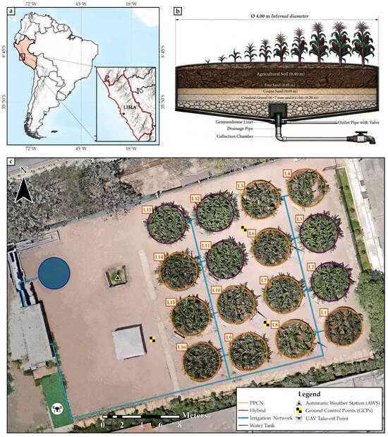
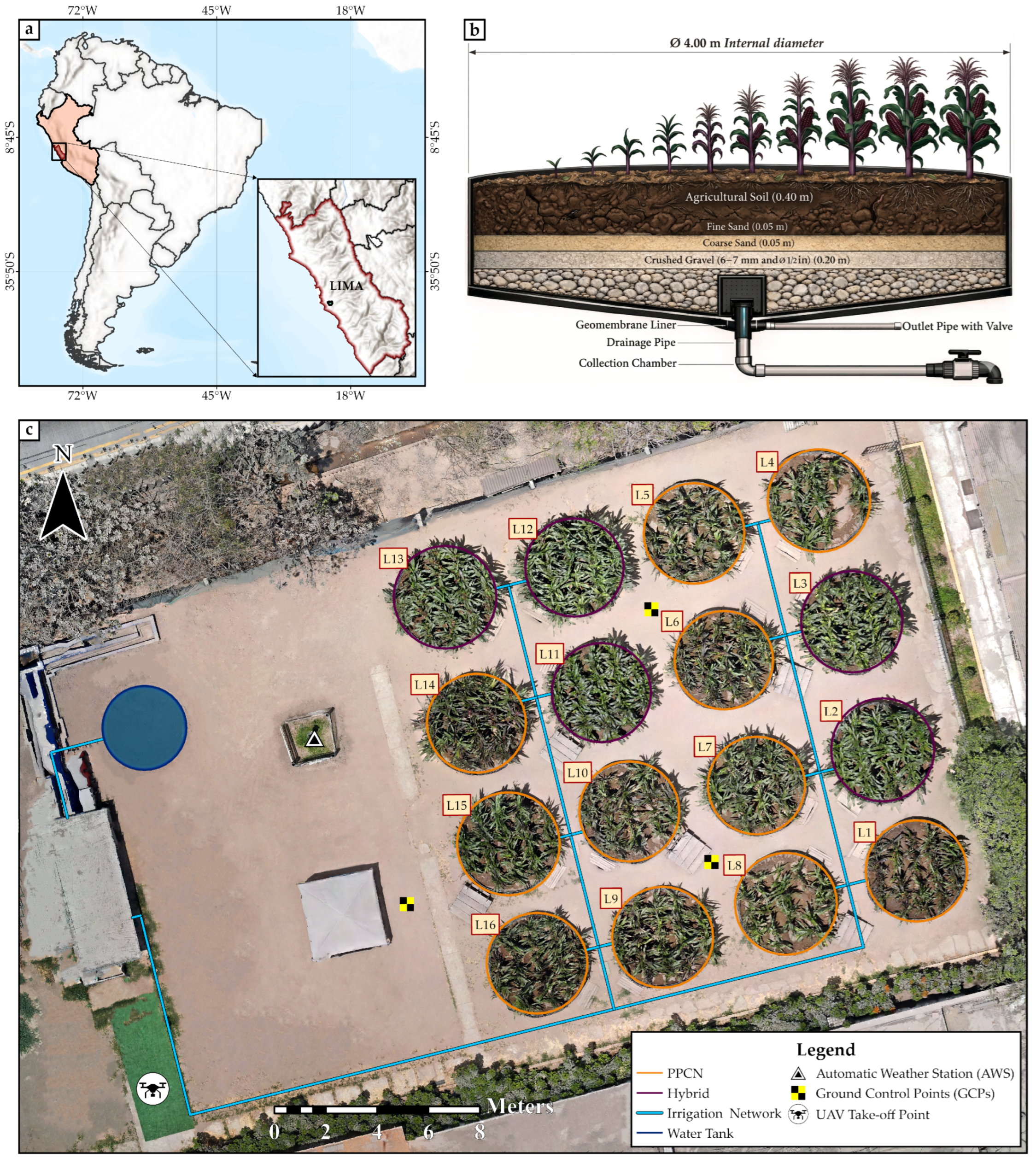
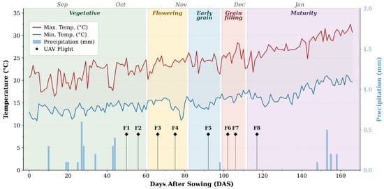
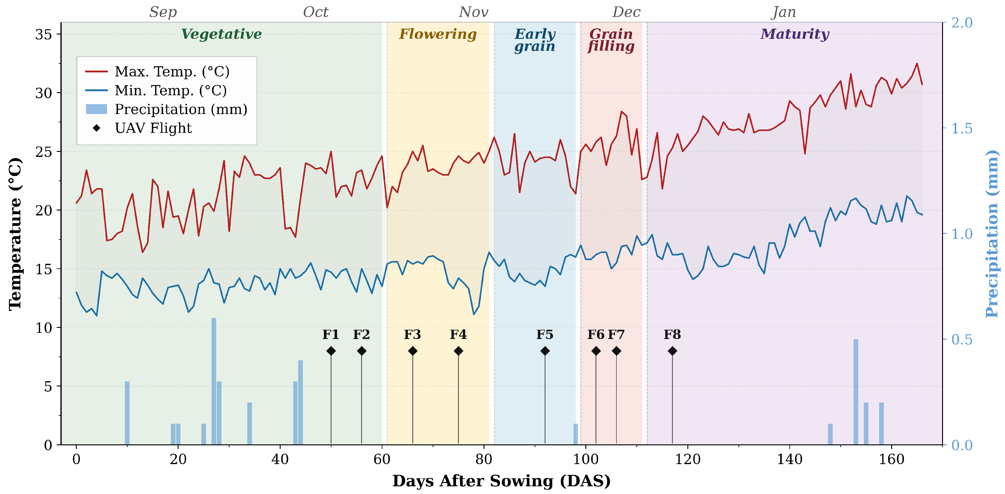
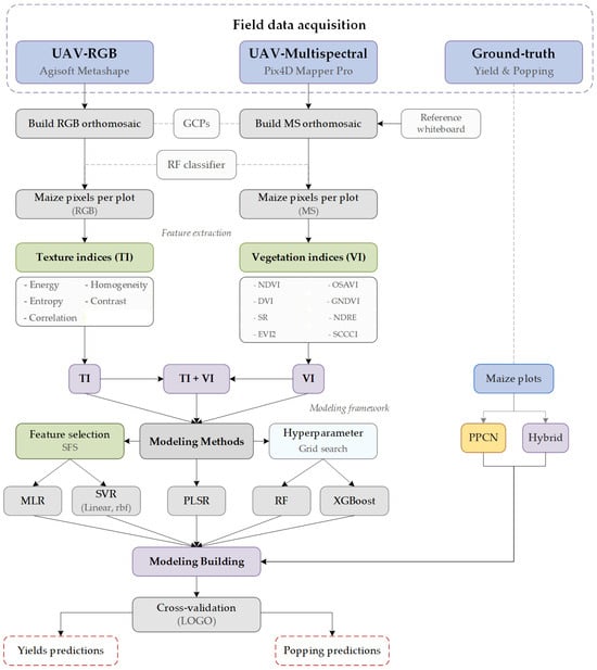
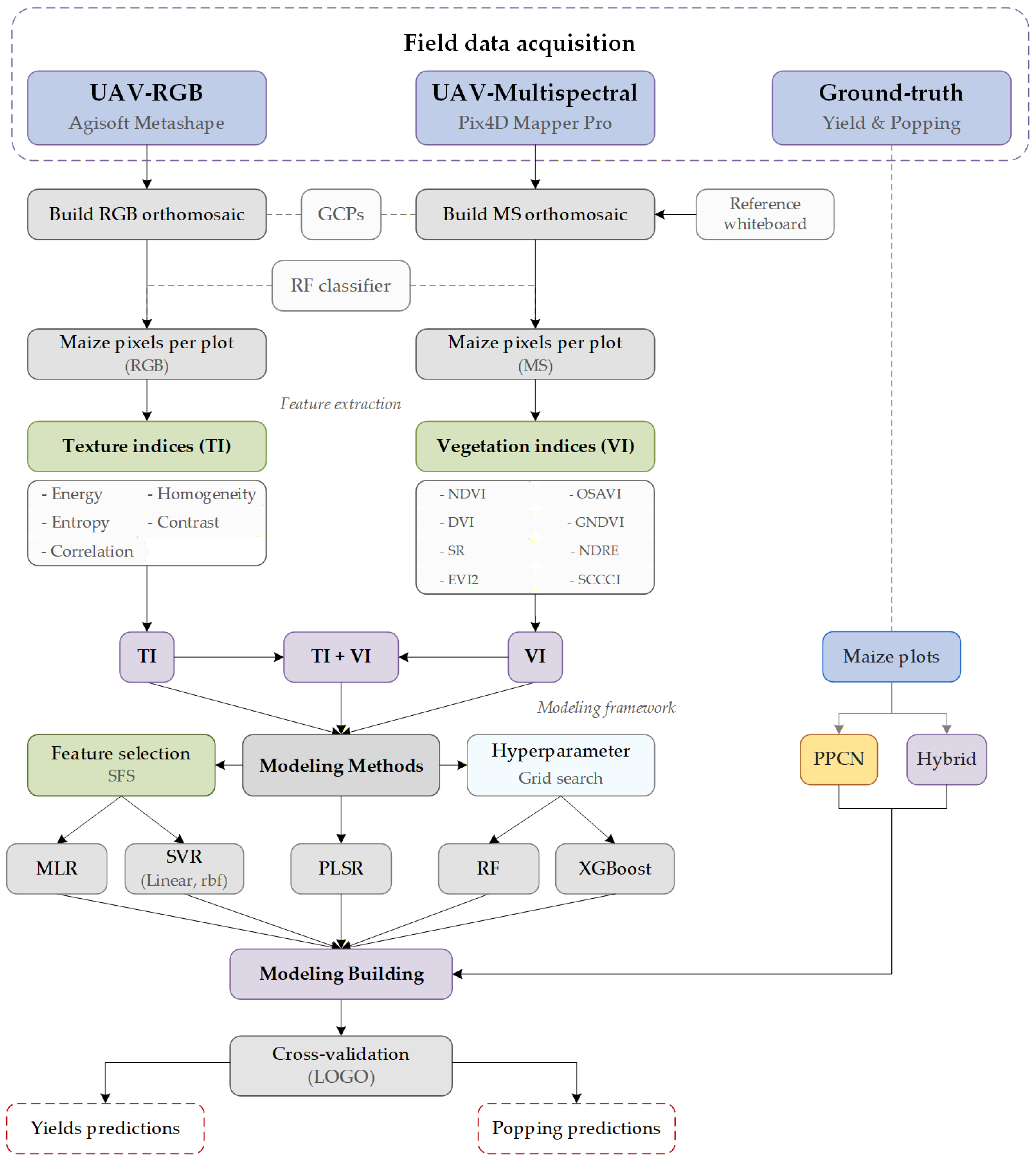
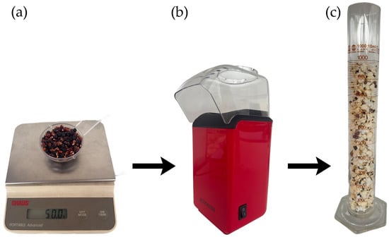
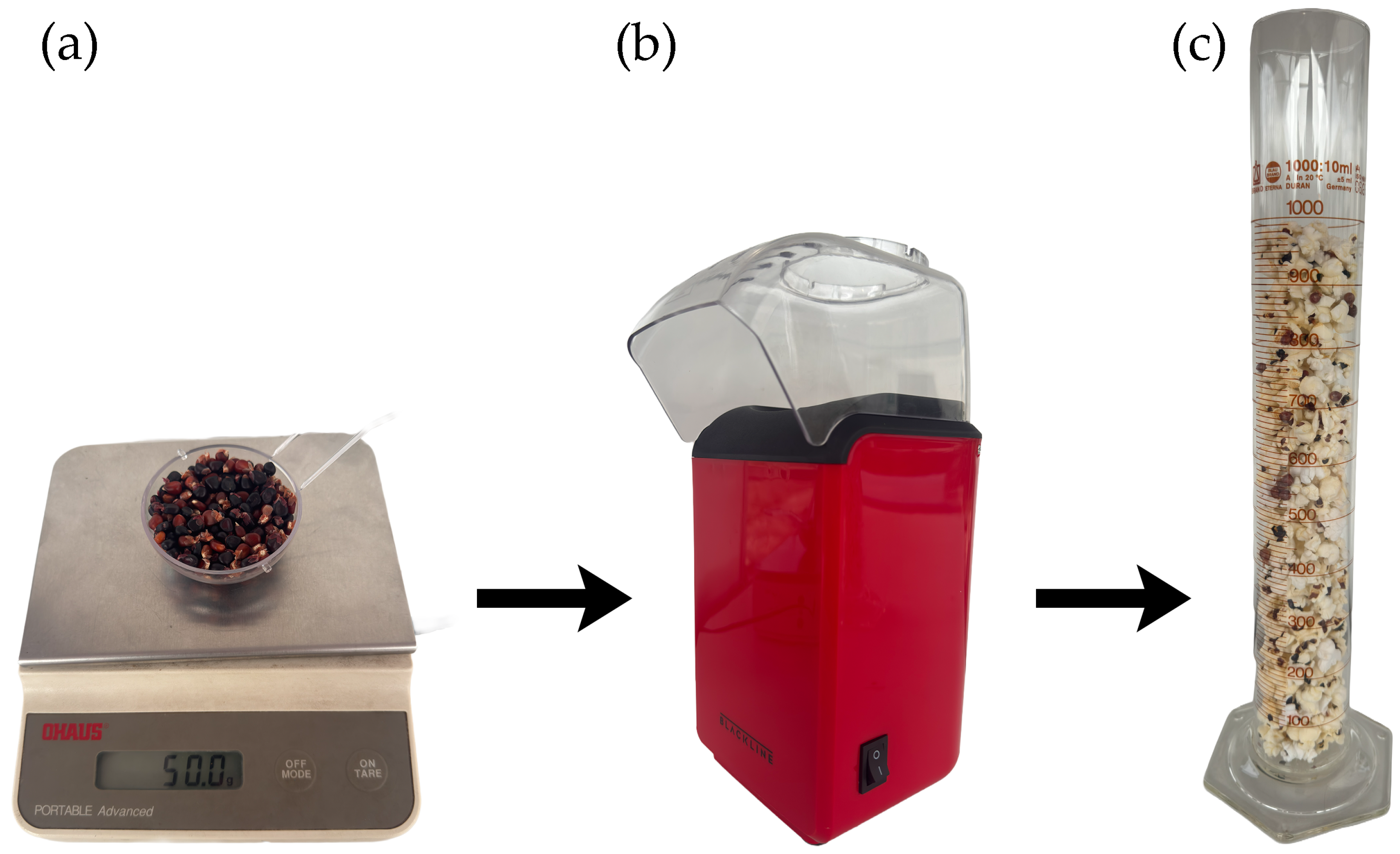
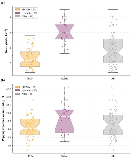
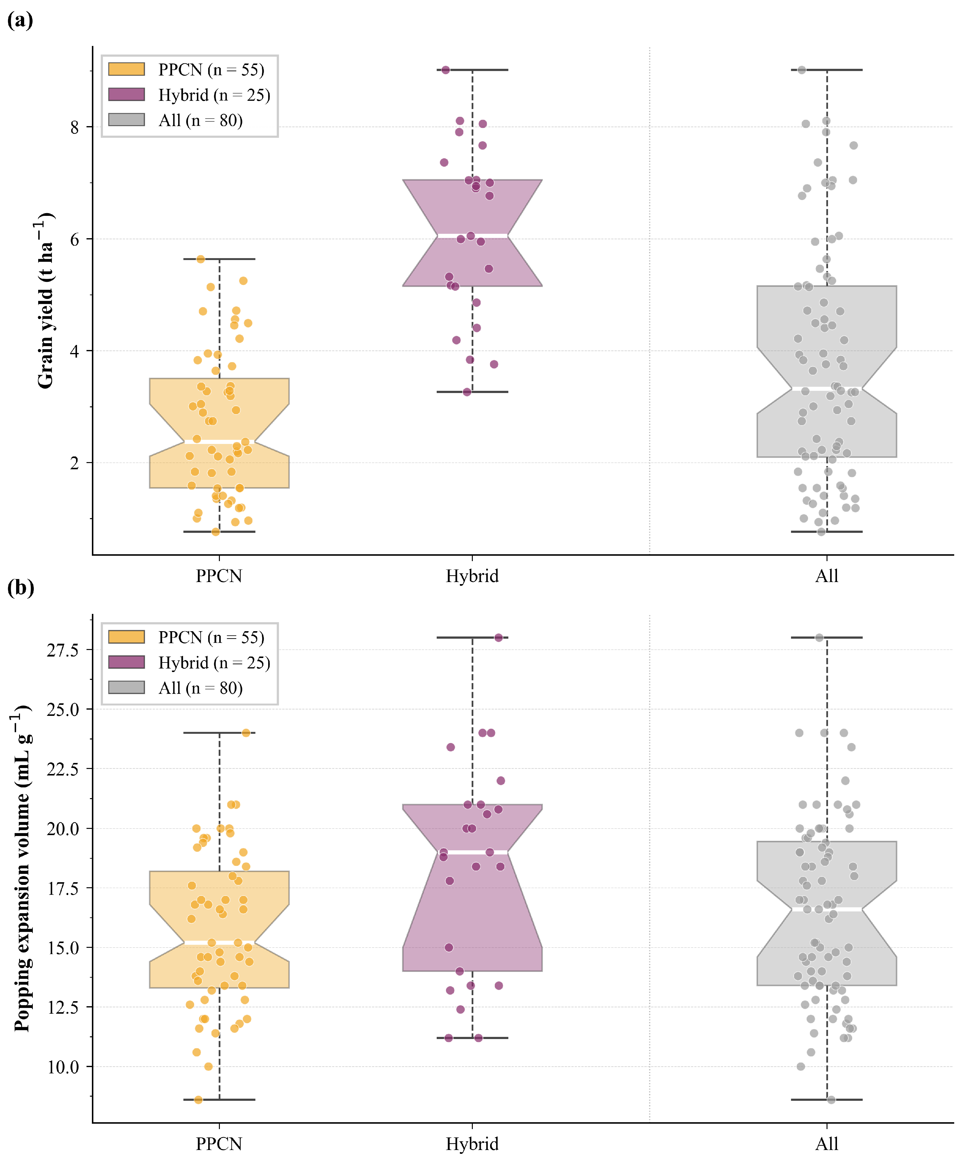
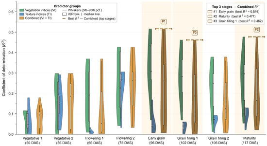
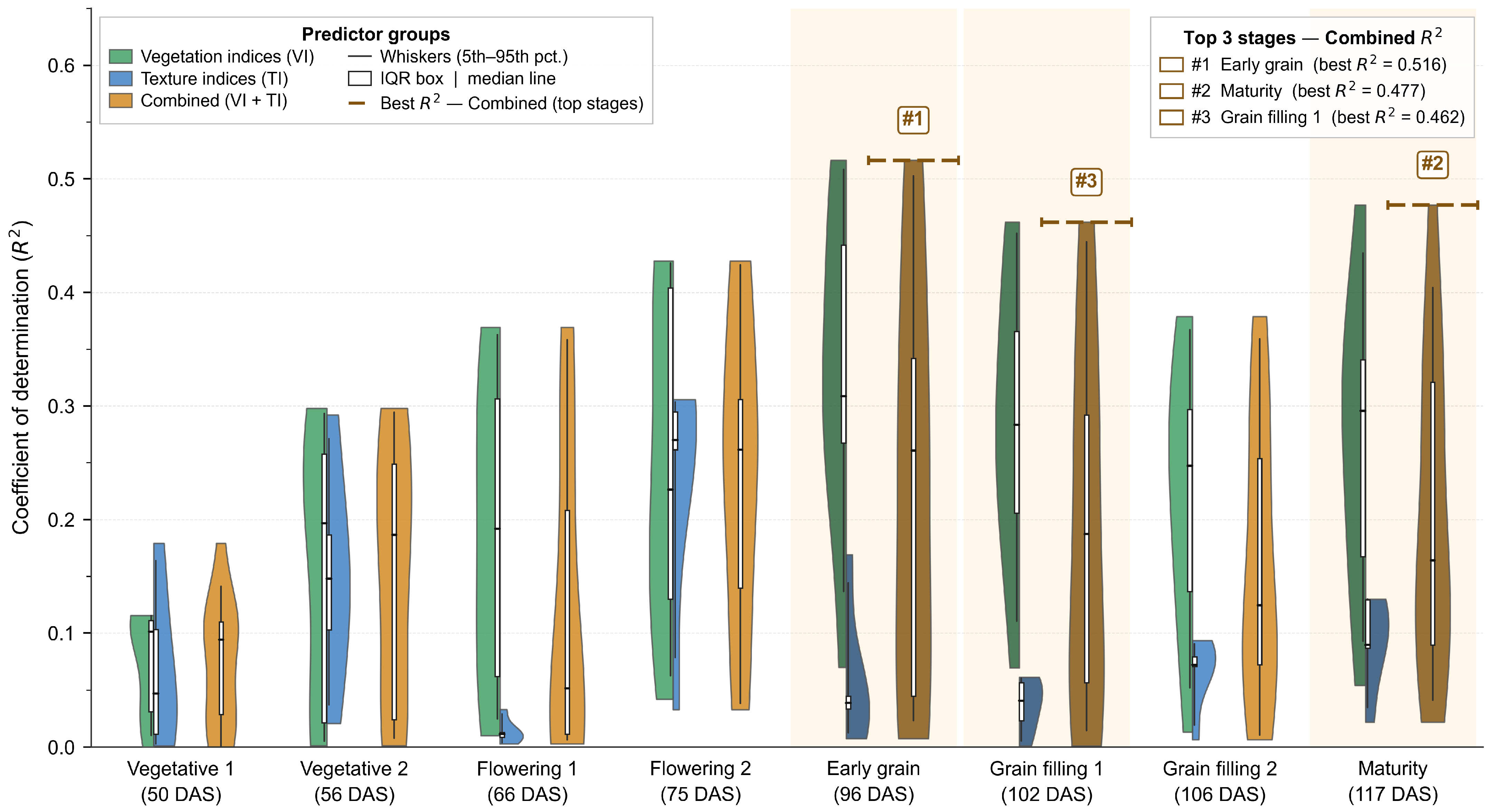
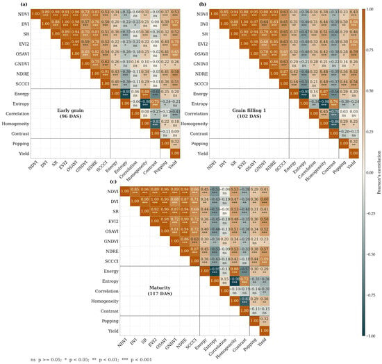
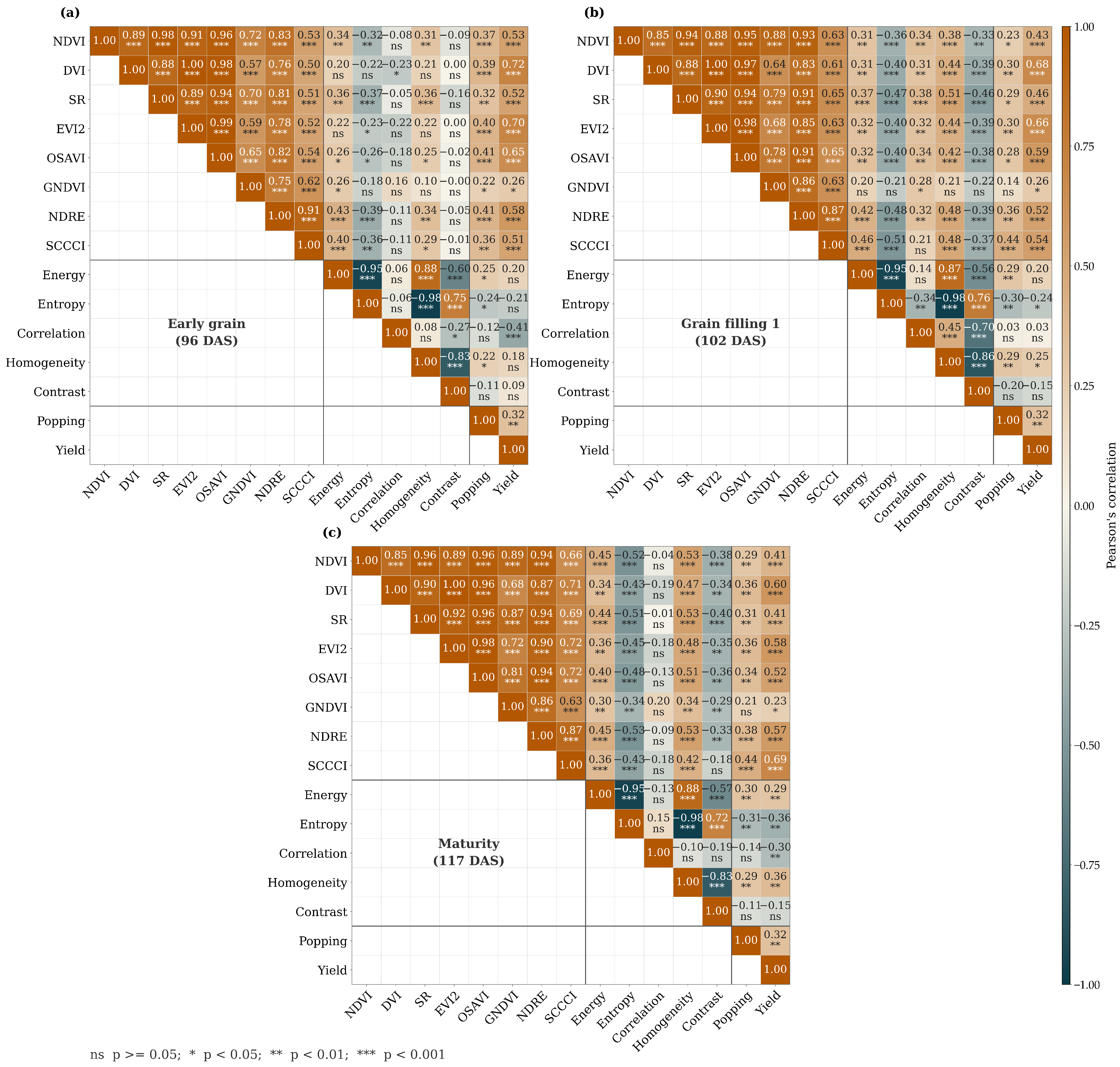
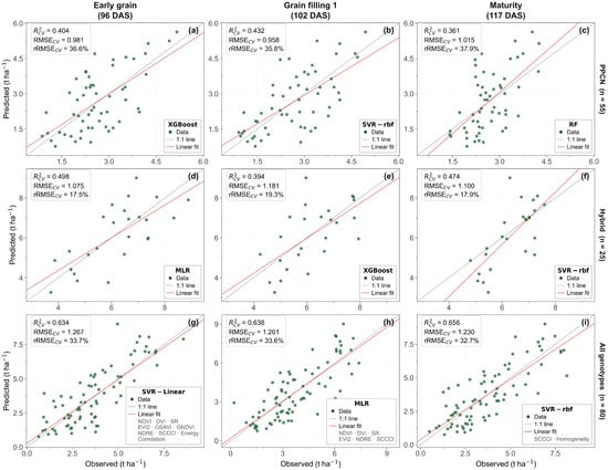
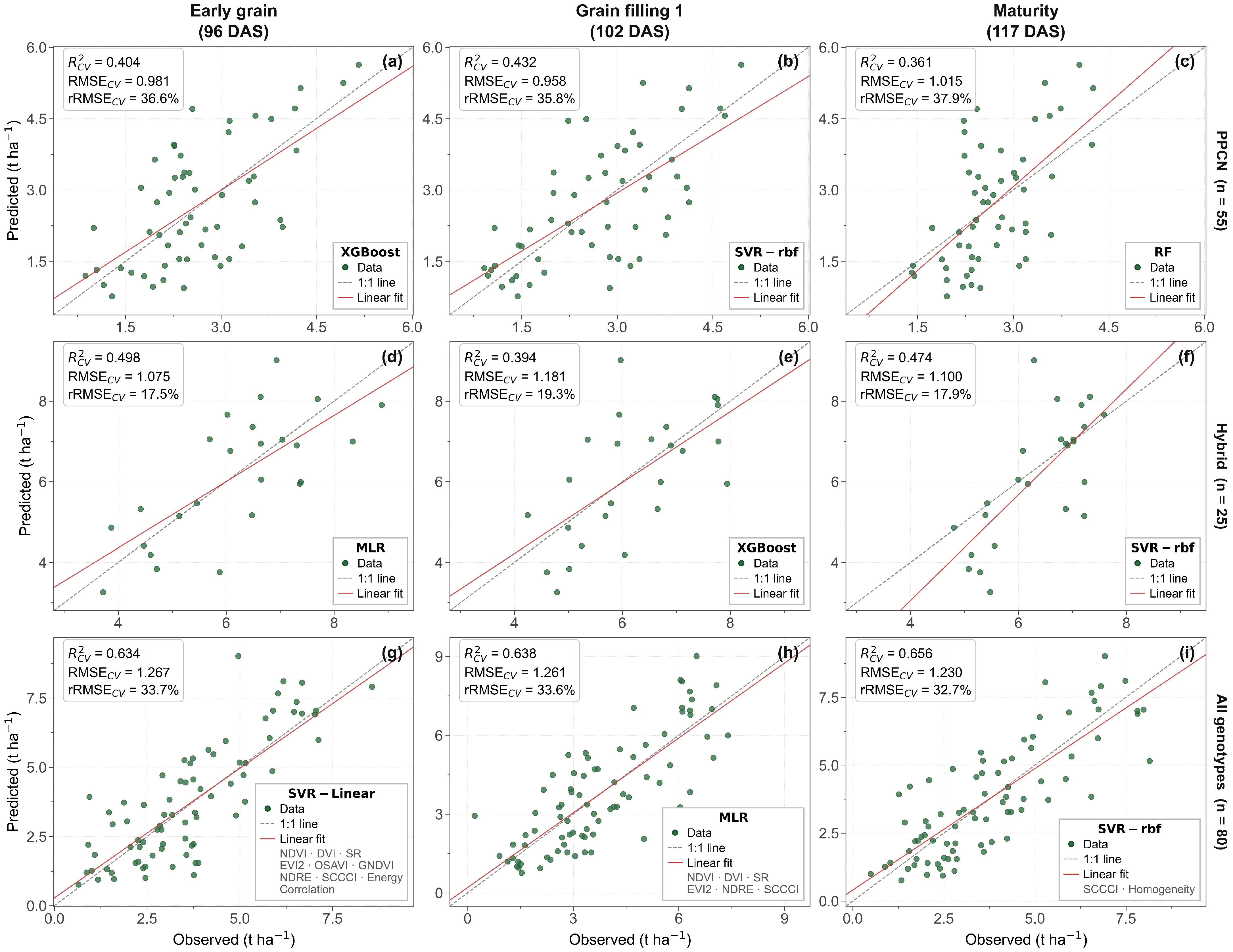
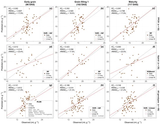
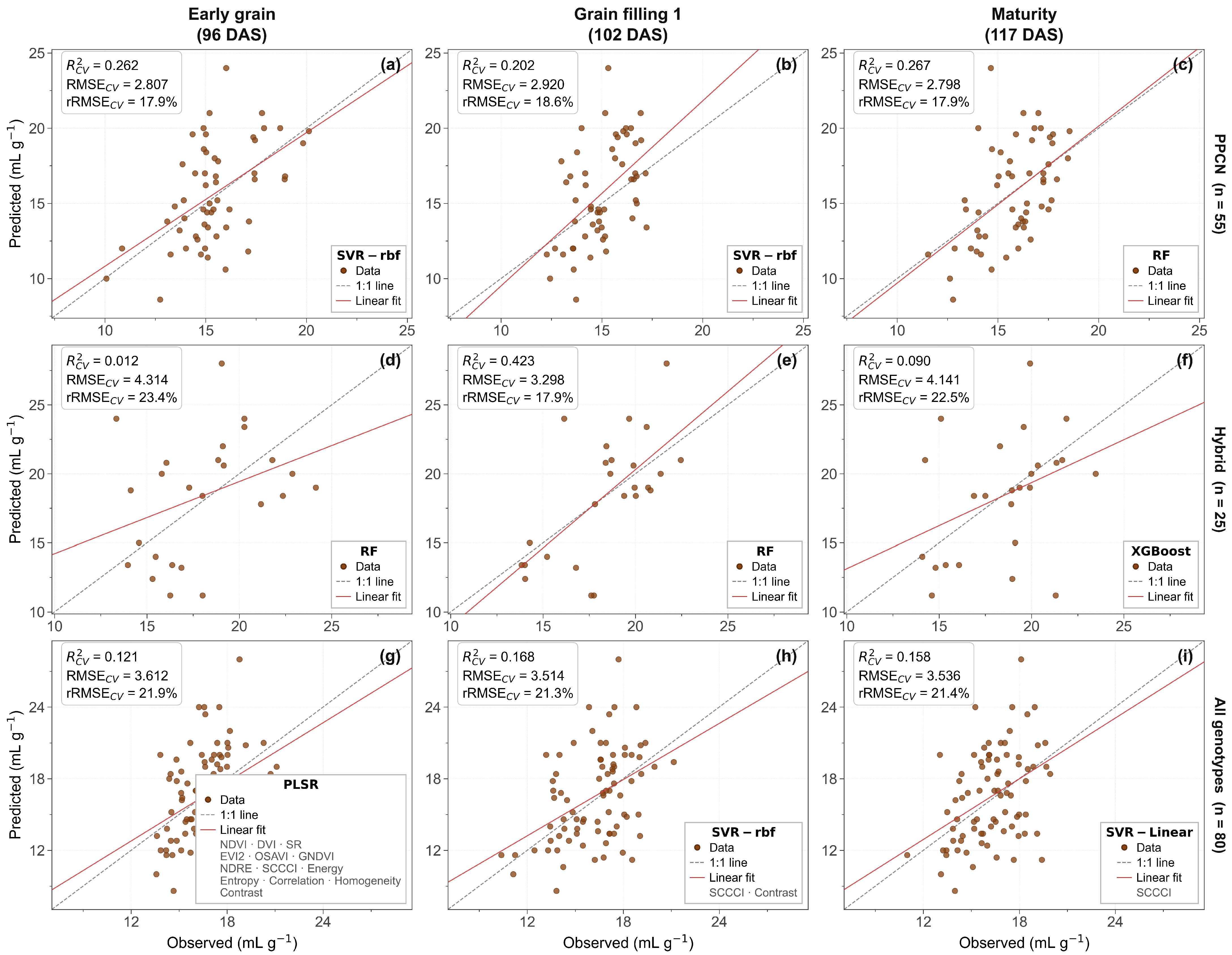
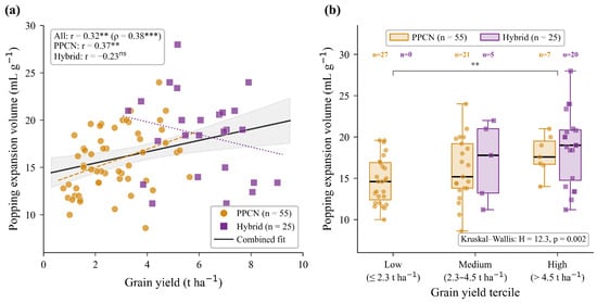
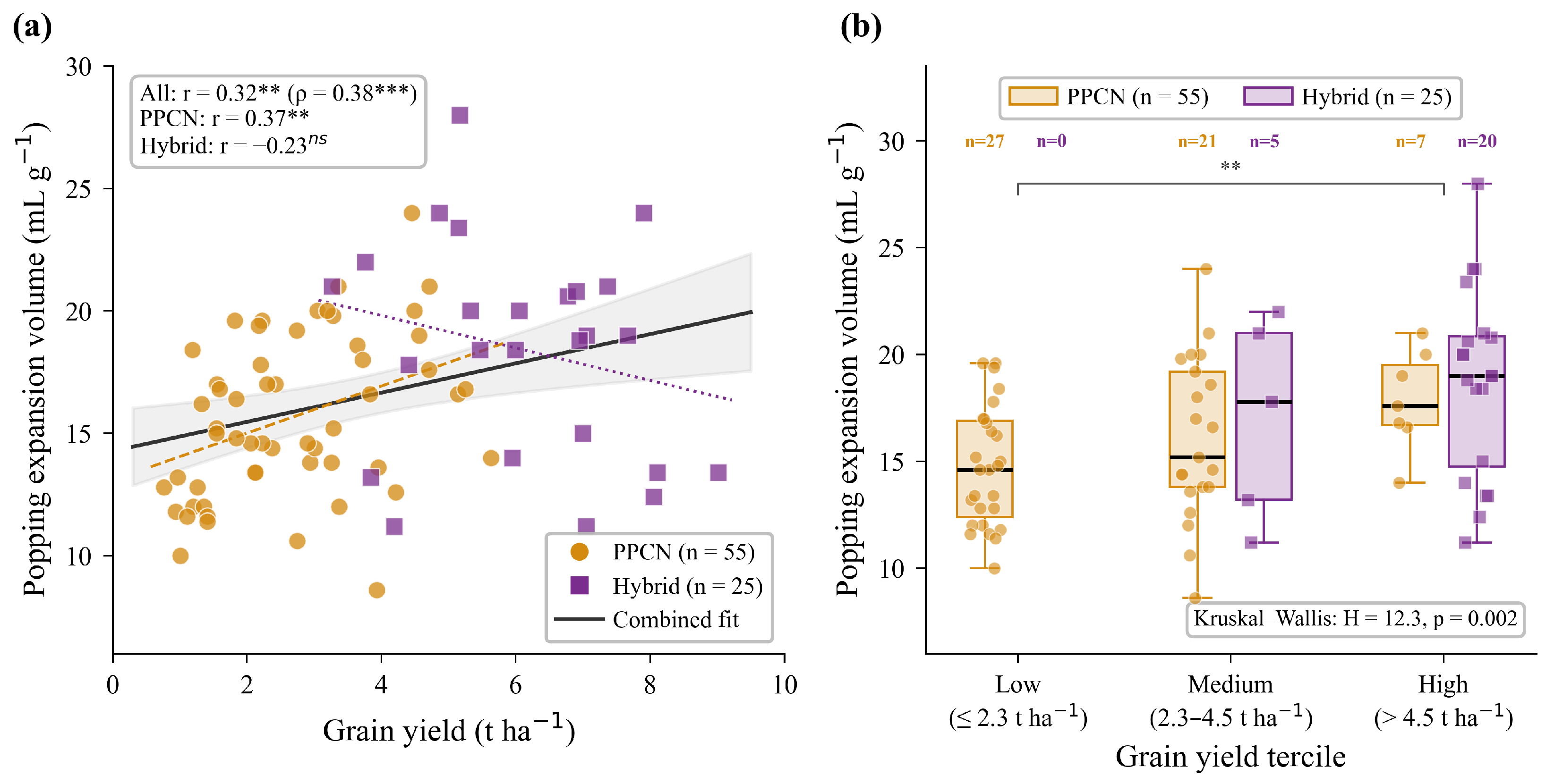

Disclaimer/Publisher’s Note: The statements, opinions and data contained in all publications are solely those of the individual author(s) and contributor(s) and not of MDPI and/or the editor(s). MDPI and/or the editor(s) disclaim responsibility for any injury to people or property resulting from any ideas, methods, instructions or products referred to in the content. |
© 2026 by the authors. Licensee MDPI, Basel, Switzerland. This article is an open access article distributed under the terms and conditions of the Creative Commons Attribution (CC BY) license.