Comparative Analysis of Explainable Spectroscopic-Fusion Models for Avocado Leaf Nitrogen Prediction

Abstract

Precise nutrient management in avocado orchards requires accurate and interpretable predictions of leaf nitrogen content. In this study, explainable machine-learning models integrating spectral reflectance (350–2500 nm) and multispectral spatial features were comparatively evaluated for non-destructive estimation of avocado leaf nitrogen content. Partial Least Squares Regression (PLSR) and one-dimensional Convolutional Neural Network (1D-CNN) models were first developed using only spectral reflectance data as a baseline. To incorporate spatial–spectral information, multispectral images were arranged into cubes and processed with a 3D-CNN to extract deep features. These features were subsequently fused with the original spectral data to form a combined dataset. Both PLSR and 1D-CNN models were retrained using the fused inputs. The CNN hyperparameters were fine-tuned using Bayesian optimization, achieving a prediction R² of 0.73 and an RMSE of 0.92 mg/g, which was comparable to the conventional PLSR model. The fusion approach showed numerically better performance than models based solely on spectra, suggesting spatial context may provide complementary information relevant to nitrogen estimation. Explainable artificial intelligence techniques, including SHapley Additive exPlanations and Integrated Gradients, identified 745 nm (red-edge), 994 nm (near-infrared), and 2459 nm (shortwave infrared), together with deep spatial features extracted from multispectral image cubes, as the most important predictors of nitrogen content in avocado leaves.

1. Introduction

Avocado (Persea americana Mill.) is an economically important fruit crop widely cultivated in tropical and subtropical regions [1]. The fruit is rich in healthy lipids, vitamins, minerals, and bioactive compounds that contribute to both human nutrition and commercial value. Among the essential nutrients required for avocado production, nitrogen plays a critical role in regulating leaf development, chlorophyll formation, photosynthetic activity, and overall plant productivity [2]. Insufficient or excessive nitrogen availability can adversely affect vegetative growth, fruit yield, and fruit quality. Therefore, accurate assessment of nitrogen status is essential for optimizing fertilizer management and improving sustainable avocado production. Conventional nitrogen determination methods, including laboratory-based chemical analyses, are often destructive, labor-intensive, time-consuming, and unsuitable for rapid field-scale monitoring [3]. Consequently, there is increasing interest in developing rapid, non-destructive, and reliable sensing techniques for nitrogen estimation in plants. In addition, machine learning-based methods for evaluating agricultural crops have been praised for their precision, non-destructiveness, and consistency of outcomes [4].

Recently, multispectral sensing technologies have emerged as powerful non-destructive tools for evaluating plant biochemical and physiological properties [5]. These techniques measure the interaction between electromagnetic radiation and plant tissues across a wide range of wavelengths, enabling the detection of subtle spectral variations associated with chlorophyll concentration, water content, nutrient composition, and internal leaf structure [5]. Because different wavelengths are absorbed or reflected based on the composition and status of the plant, spectral reflectance reveals the biochemical and physiological state of the plant [6]. In particular, multispectral reflectance data in the visible, red-edge, near-infrared (NIR), and shortwave infrared (SWIR) regions have shown strong sensitivity to plant nitrogen status because nitrogen is closely associated with chlorophyll absorption and protein-related biochemical features [7]. Recent studies have demonstrated the potential of multispectral imaging (MSI) and spectroscopic analysis for predicting nitrogen content in various agricultural crops [8]. In addition to spectral information, MSI can provide spatial information on leaf texture, venation patterns, and structural heterogeneity, which may further improve nitrogen estimation accuracy. These advantages make MSI a promising approach for rapid and non-destructive assessment of plant nitrogen content.

Despite the strong potential of multispectral sensing for nitrogen assessment, many conventional spectroscopic approaches rely primarily on spectral information alone and often overlook the spatial characteristics present within MSI cubes. Conventional chemometric models such as partial least squares regression (PLSR) have been widely applied for nutrient prediction because of their simplicity and interpretability [9]. However, such approaches may not fully capture the complex nonlinear relationships between spectral responses and plant biochemical properties. In addition, spectral-only models generally ignore important structural and spatial information associated with leaf morphology, venation, internal organization, and texture variability, all of which can influence reflectance behavior and nutrient estimation. Since MSI cubes inherently contain both spectral and spatial information, utilizing only spectral reflectance may limit the predictive capability of nitrogen estimation models. Therefore, integrating spectral and spatial information has gained increasing attention as a strategy to improve the robustness and accuracy of plant trait prediction models [10,11].

Recent advances in deep learning have opened new opportunities to extract complex spectral–spatial relationships from multispectral datasets. Convolutional neural networks (CNNs), in particular, have demonstrated strong capability in automatically learning hierarchical features from high-dimensional data without extensive manual feature engineering [12]. One-dimensional CNNs (1D-CNNs) have been successfully applied to spectroscopic data analysis because convolutional filters can effectively capture informative spectral patterns related to biochemical composition [13]. Similarly, three-dimensional CNNs (3D-CNNs) are especially suitable for multispectral image analysis because they can simultaneously learn spatial and spectral representations from image cubes [14]. Previous studies have shown that combining spectral reflectance with spatial features extracted through CNN architectures can significantly improve predictive performance in agricultural applications [10]. Furthermore, multimodal data fusion strategies, including feature concatenation, weighted fusion, and attention-based fusion, have been increasingly explored to integrate complementary information from different sensing modalities [15]. Although attention mechanisms theoretically allow adaptive weighting of informative features, their performance may depend heavily on dataset size and model complexity. Consequently, a comparative evaluation of different fusion strategies remains important for identifying robust, practical approaches to multispectral sensing for crop analysis.

While deep learning models often achieve high predictive accuracy, their decision-making processes are frequently difficult to interpret because they operate as complex “black-box” systems. In agricultural applications, model interpretability is important for improving scientific understanding, increasing user confidence, and identifying biologically meaningful spectral regions associated with plant traits [16]. Explainable Artificial Intelligence (XAI) techniques such as SHapley Additive exPlanations (SHAP) and Integrated Gradients (IG) [17] have recently gained attention for interpreting deep learning predictions by identifying influential wavelengths and spatial regions contributing to model outputs. SHAP analysis can quantify the contribution of individual spectral features to prediction outcomes, while IG-based visualization methods can highlight important spatial regions learned by CNN architectures [16]. Despite growing interest in explainable deep learning for multimodal data analysis, a few prior studies have used spectral–spatial or hyperspectral imaging approaches for nitrogen prediction [18,19,20]. However, to the best of our knowledge, no studies have integrated spectral–spatial fusion with XAI for avocado leaf nitrogen prediction. In particular, there is insufficient understanding of how fused spectral and spatial features contribute to nitrogen estimation and how different fusion strategies influence model performance and interpretability.

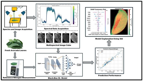
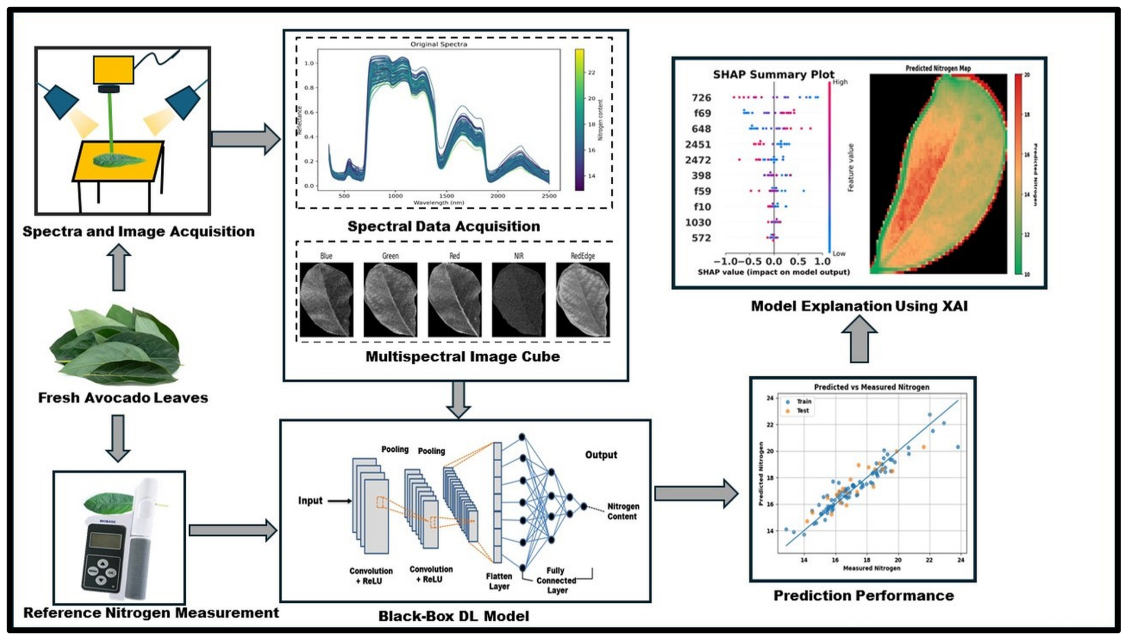
Therefore, the objective of this study was to develop and compare explainable spectral–spatial fusion models for predicting nitrogen content in avocado leaves using full-range Ultraviolet–visible–near infrared (UV–VIS–NIR: 350–2500 nm) reflectance spectroscopy and MSI data. Specifically, this study aimed to: (i) develop PLSR and 1D-CNN models using spectral reflectance and fused spectral–spatial features; (ii) compare multiple fusion strategies, including feature concatenation, weighted fusion, and attention-based fusion; and (iii) interpret the developed models using SHAP and IG to identify influential spectral wavelengths and spatial features contributing to nitrogen prediction. The overall workflow of the proposed spectral–spatial fusion framework for avocado leaf nitrogen prediction is illustrated in (Figure 1). The findings of this study are expected to support the development of more reliable and interpretable sensing frameworks for non-destructive nutrient assessment in precision agriculture.

Figure 1. Overall workflow of the proposed methodology for avocado leaf nitrogen prediction using a fusion model and an XAI.

2. Materials and Methods

The methodology consists of reflectance spectra acquisition, reference parameter analysis, multispectral image cube generation, spectral–spatial feature extraction, fusion-based model development, and XAI analysis for the interpretation of influential spectral and spatial features. Detailed descriptions of each processing stage are provided in the following subsections.

2.1. Collection of Avocado Leaves

Avocado leaf samples representing one of the most widely cultivated cultivars in the Valparaíso region of Chile were utilized in this study [21,22]. Leaf sampling was conducted during April and May 2023, and a total of 104 leaf samples were collected. Individual branches were cut directly from the trees, and leaves were selected based on visual assessment of physical integrity and overall condition. Leaves exhibiting severe physical damage, internal ruptures, extensive discoloration, or pronounced deterioration symptoms were excluded from the analysis. Minor surface defects were considered acceptable provided that the majority of the leaf area remained unaffected. Following collection, the samples were placed in sealed bags and transported to the laboratory for reflectance measurement, multispectral image acquisition, and reference nitrogen analysis.

2.2. Spectral Data Collection

Spectral reflectance measurements were conducted using an ASD TerraSpec Hi-Res Spectrometer (Malvern Panalytical, Malvern, UK), which captures data across a wavelength range of 350–2500 nm [21]. Prior to measurement, the instrument was warmed up for 15 min and adjusted with a white Spectralon panel to ensure accuracy. To collect the spectra, each leaf sample is placed on a white Spectralon background with the contact probe flat against it. For each leaf, three spectral readings were taken at the bottom, middle, and top regions (Supplementary Information, Figure S1), which were subsequently averaged to obtain a single representative reflectance value. The spectrometer was recalibrated after measuring all sets of leaves at each phase to maintain data integrity. Throughout the measurement sessions, the laboratory environment was controlled, with temperatures maintained between 20–25 °C and relative humidity between 55–70%.

2.3. Multispectral Image Acquisition and Image Correction

Multispectral images were acquired using a MicaSense RedEdge camera (MicaSense Inc., Seattle, WA, USA) was positioned 45 cm above the samples on a tripod. Four avocado leaves were arranged in limited amounts on a white paper background [21]. To ensure controlled illumination and minimize interference from natural light, windows were blocked, and artificial lighting was provided by ceiling-mounted fluorescent lamps (4100 K, 2850 lm). To ensure image quality and consistency, a series of post-processing steps was applied. Radiometric adjusting was initially carried out for each spectral band using metadata and reference imagery of a calibrated reflectance panel obtained in each trial, implemented via MicaSense Python-based software provided by Micasense (https://github.com/micasense/imageprocessing, accessed on 31 October 2026). Subsequently, segmentation and binarization were conducted to isolate individual leaves. An Otsu-based thresholding method was used to generate binary images and extract leaf contours [23]. These contours were then used to mask and crop to obtain individual leaf images. Finally, manual refinement was performed in MATLAB Image Segmenter (MATLAB R2024a) to correct errors such as overlapping leaves and misclassified regions, ensuring accurate leaf extraction [21].

2.4. Reference Nitrogen Measurement

After spectral data and image acquisition, the nitrogen content of the avocado leaves was assessed with a TYS-4N Plant Nutrition Meter (Zhejiang TOP Cloud-agri Technology Co., Ltd., Hangzhou, China). The device measures nitrogen non-destructively and outputs the content in mg/g over a measuring range of 0.0–99.9 mg/g, eliminating the need for an external conversion formula. It has a measurement accuracy of ±5% and a repeatability of ±0.5 units. Three readings were obtained from the bottom, middle, and top regions of each leaf, and the measurements were averaged to improve consistency. Furthermore, the nutrition meter was recalibrated after each batch to ensure the reliability of the collected reference data [21]. This study did not validate against a conventional chemical method (Kjeldahl or Dumas), hence the ±5% accuracy is based on the manufacturer’s specification.

2.5. Development of Multimodal Fusion Data

The Kennard–Stone (KS) algorithm [24] was used to partition the 104 avocado leaf samples into calibration (n = 83, 80%) and prediction (n = 21, 20%) sets prior to developing the fusion dataset. The KS algorithm is an iterative process that samples the spectral feature space uniformly and representatively by selecting samples with a maximum Euclidean distance in the N dimensional spectral space. Starting from the two most different samples, each new sample is chosen to be as far as possible from each of the previously selected samples. In this manner, the selection is structured so that the calibration set will contain all of the dataset’s spectral variability, which is necessary especially for small datasets like the 104 avocado leaf samples in this work. This technique guarantees that samples encompass a broad spectrum of variability, acquiring unique and varied data points for thorough analysis [25]. To ensure data integrity across all modalities, the same partition was used for both spectral reflectance data and the multispectral image cubes based on KS.

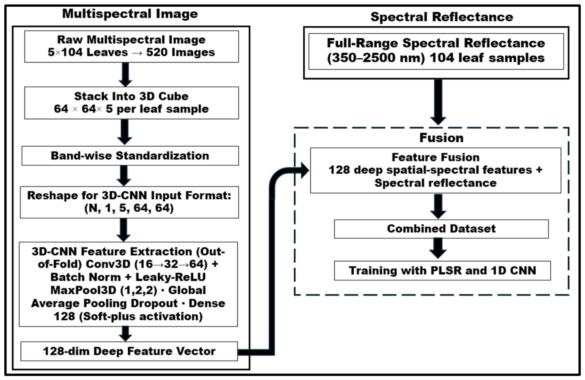
The complete fusion procedure was: (1) Dividing the 104 leaf samples into two subsets, calibration (n = 83) and prediction (n = 21) using the KS algorithm. (2) Stacking 5-band multispectral images to 3D cubes of size (64 × 64 × 5) for each subset. (3) To limit information leakage during feature extraction, the calibration subset was subjected to 3D-CNN-based spatial feature extraction with a five-fold out-of-fold (OOF). Specifically, the 83 calibration samples were separated into five folds. For each fold, the 3D-CNN was trained on the training folds, and 128-dimensional characteristics were recovered for the associated held-out fold. This procedure was repeated until OOF features were created for all calibration samples. For the independent prediction subset, 128-dimensional features were extracted using each of the five-fold trained 3D-CNN models, and the resulting feature vectors were averaged across the five models to produce the final features. Thus, each calibration sample’s feature vector was retrieved using a 3D-CNN that had not been trained on that sample, eliminating the possibility of information leakage and optimistic bias during feature extraction. (4) Concatenating the OOF calibration features and the independent prediction features with the corresponding full-range (350–2500 nm) spectral reflectance data. (5) Training the downstream prediction models, PLSR and 1D-CNN with 5-fold cross-validation.

To capture joint spatial–spectral information, a three-dimensional convolutional approach was adopted in this investigation. A 3D-CNN feature-extraction pipeline was developed for multispectral leaf-image analysis. Images in 5 spectral bandsblue, green, red, NIR, and red-edge were obtained for each leaf sample and stacked to create a 3D cube of size (64 × 64 × 5). There were 104 avocado leaf samples, and each leaf was provided with five multispectral band images. All multispectral images utilized in this study were captured at the fresh stage.

The suggested architecture uses 3D convolutional layers to process individual spatio–spectral feature-rich cubes from multispectral pictures [26], with base, base × 2, and base × 4 filter sizes, respectively, where base filter size was used as a tunable hyperparameter. The first convolutional layer has a kernel size of (5, 3, 3) and is utilized in the five-band cube over the entire spectral depth, with 3 × 3 spatial convolution, the second and third convolutional layers have a kernel size of (3, 3, 3). All convolutional layers are followed by Batch Normalization and LeakyReLU (0.1) activation to improve training stability and reduce dead activations. MaxPool3D layers of the form (1, 2, 2) were used to perform spatial downsampling as opposed to spectral depth. Then the learned spatio–spectral representations were compressed into a small feature vector with global average pooling. A dropout layer was placed in front of the fully connected embedding layer to reduce the overfitting problem. A 128-unit, Softplus-activated dense layer was used to generate a 128-dimensional non-negative feature embedding for each leaf sample. Instead of cube-level min-max normalization, band-wise standardization was applied using statistics computed only from the calibration set, ensuring that each spectral band was normalized independently while preventing data leakage from the prediction set. The dataset was then reshaped to the 3D-CNN input format (N, 1, 5, 64, 64), with the spectral bands arranged along the depth dimension and a single input channel. The values of 3D-CNN hyperparameters (base filter size, dropout rate, learning rate and weight decay) were obtained by optimizing them through Bayesian optimization using a Tree-structured Parzen Estimator sampler [13]. A search was performed over 30 trials (patience = 8) trained for up to 50 epochs. The final model was retrained with hyperparameters that were best identified for 60 epochs with the Adam optimization method and mean squared error (MSE) loss. The combined dataset comprising full-range spectroscopic reflectance data (350–2500 nm) from the ASD spectrometer and 128 deep features derived from MSI was used for training the prediction models (PLSR and 1D-CNN) so that a comparison could be made between the traditional chemometric solution and the deep learning solution. This fusion strategy is effective because 3D-CNNs are able to jointly exploit spectral and spatial information by performing convolutions in both spatial and spectral dimensions [27].

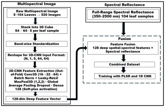
Additionally, two other types of fusion strategies (weighted feature fusion and attention-based feature fusion) were also demonstrated. Prior to concatenation, the weighted fusion [15] involved multiplying the standardized spectral and spatial feature matrices by fixed scalar weights (0.7 and 0.3, respectively). The attention-based fusion [28] used a dual-branch architecture, with a 1D-CNN branch processing spectral data and a multilayer perceptron (MLP) branch processing spatial data. The embeddings from both branches were concatenated and fed into an MLP-based Softmax attention mechanism, which dynamically computed per-sample importance weights. The proposed feature-level fusion architecture is illustrated in (Figure 2).

Figure 2. Proposed feature-level spectroscopic fusion architecture combining deep spatial features extracted by 3D-CNN with full-range spectral reflectance data.

2.6. Development of Spectral and Fusion-Based Prediction Models

Before model development, Savitzky–Golay smoothing [24], which included first derivative transformation was used on spectral data to highlight fine spectral patterns and lower the impact of noise in the data. This preprocessing was applied consistently prior to the development of both the PLSR and 1D-CNN models.

2.6.1. PLSR

PLSR, a popular chemometric technique that efficiently handles highly multicollinear data by projecting the spectrum matrix (X) and response attribute (Y) onto latent variables (LVs) to maximize covariance, was first used to calibrate the spectral dataset [29]. To avoid underfitting and overfitting, the ideal number of LVs was found by reducing the root-mean-square error [16]. To find the best model components, 3–30 components were evaluated using 5-fold cross-validation, and the number of components that minimized RMSECV without evidence of overfitting was selected [24]. This optimization was carried out separately for datasets with only reflectance values (spectral-only) and for datasets with 128 spatial features derived from the 3D-CNN (fused spectral–spatial).

2.6.2. 1D-CNN

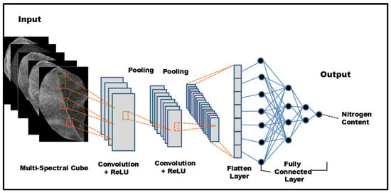
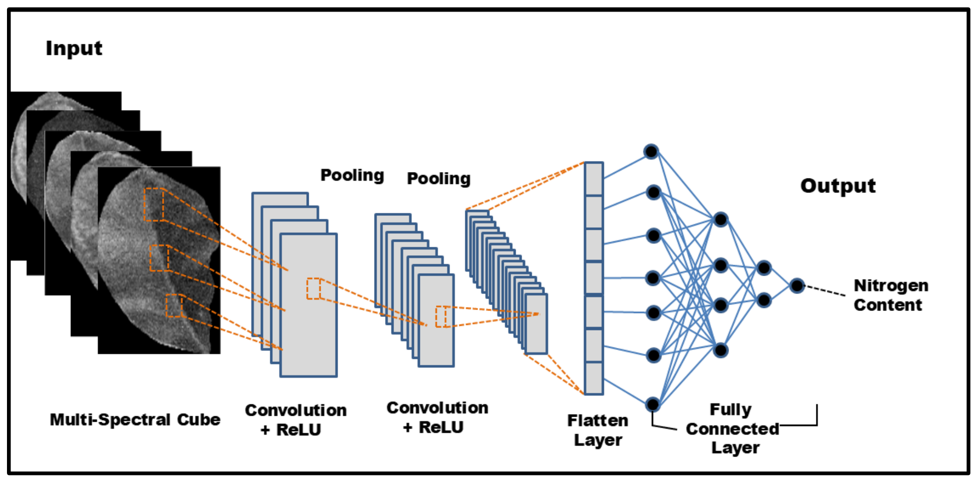
For spectroscopic analysis, a one-dimensional (1D) CNN model was created, as shown in (Figure 3). The rectified linear unit (ReLU) activation function is used in the model’s convolutional layer, two fully connected layers, and one maximum pooling layer (MaxPool). As with previous regression models, the model’s output shape of (1, 1) shows that it predicts a single continuous variable. Before arriving at an output dense layer with a single unit that uses the ReLU activation function to estimate nitrogen content, the spectral features retrieved by the convolution layer are concatenated and sent via pairs of hidden dense and dropout layers. CNN models with a single convolutional layer are frequently employed in spectroscopic analysis [13]. The convolutional layer finds prominent data patterns, and later layers create more intricate abstractions of these patterns [12]. The number of filters ensures adequate representation capability. The dataset was divided into 80% for calibration and 20% for prediction, consistent with the KS partition described in Section 2.5. To produce a robust and unbiased evaluation of model performance, the calibration set (80%) was trained using a 5-fold cross-validation method, with four folds utilized for training and the fifth fold for validation in each iteration. A Bayesian optimization approach, which effectively searches the hyperparameter space, was used to fine-tune the hyperparameters, which include filter size, kernel size, pool size, batch size, number of epochs, and learning rate. When assessing the objective function is computationally costly, Bayesian optimization is beneficial. The Bayesian optimization approach uses kernel density estimators to estimate the probability densities of “good” and “bad” hyperparameter configurations rather than directly modeling the objective function [13]. Table 1 provides specifics about the input hyperparameter space used in this investigation. Model weights and biases were optimized using the Adam algorithm and the model was trained for up to 250 epochs with Early Stopping (patience = 20) to avoid overfitting. Importantly, the Bayesian hyperparameter optimization was carried out separately for the spectral-only dataset and fused spectral–spatial dataset. The datasets were considered individually and optimized separately, resulting in data-specific optimal architectures for the different feature structures and dimensionalities of the datasets. This means that the performance results reported for each model correspond to the architecture optimized for their input data, not to a common set of parameters used for both scenarios.

Figure 3. Architecture of 1D-CNN model.

Table 1. Hyperparameter search space for the proposed 1D-CNN model.

Hyperparameter	Range/Value
Epochs (max_epochs)	250 (early stopping, patience = 20)
Batch size	16
Filter—conv1_filters	16 to 64 (step 16)
Kernel size—conv1_kernel	3 or 5
Filter—conv2_filters	32 to 128 (step 32)
Kernel size—conv2_kernel	3
Dense units—dense_units	32 to 128 (step 32)
Dropout rate (block 1)	0.3 to 0.6 (step 0.1)
Dropout rate (block 2)	0.3 to 0.6 (step 0.1)
Dropout rate (dense)	0.4 to 0.6 (step 0.1)
Weight decay	1 × 10−6 to 1 × 10−2 (log scale)
Learning rate	1 × 10−4 to 5 × 10−3 (log scale)
Pooling layer	MaxPool1d (kernel size = 2)
Calibration/prediction split	Kennard–Stone; test size = 0.20
Loss function	Mean squared error (MSELoss)

2.7. Model Evaluation

The performance of these models is typically assessed using the Coefficient of Determination (R²), the Root Mean Squared Error (RMSE), and Relative Prediction Deviation (RPD), as given in Equations (1)–(3).

The R² value indicates how closely the predicted values align with the true values. An R² value close to 1 means the model makes highly accurate predictions, while a value near 0 suggests poor predictive performance.

$${\mathrm{R}}^2=1-{\displaystyle \frac{{\sum }_{\mathrm{i}=1}^{\mathrm{n}}{\left({\mathrm{y}}_{\mathrm{i}}-{\widehat{\mathrm{y}}}_{\mathrm{i}}\right)}^2}{{\sum }_{\mathrm{i}=1}^{\mathrm{n}}{\left({\mathrm{y}}_{\mathrm{i}}-\overline{\mathrm{y}}\right)}^2}}$$

(1)

The average size of the discrepancies between expected and actual values is measured by the RMSE. Higher coefficients of determinations together with lower error values were considered indicative of better model performance [30].

$$\mathrm{RMSE}=\sqrt{{\displaystyle \frac{{\sum }_{\mathrm{i}=1}^{\mathrm{n}}{\left({ {\widehat{\mathrm{y}}}_{\mathrm{i}}-\mathrm{y}}_{\mathrm{i}}\right)}^2}{\mathrm{n}}}}$$

(2)

RPD measures the ratio of the variability in the true values to the prediction error. A higher RPD indicates that the model has better predictive performance and reliability, as the predictions capture more of the true data variation compared to the error.

$$\mathrm{RPD}={\displaystyle \frac{{\mathrm{\sigma }}_{\mathrm{y}}}{\mathrm{RMSEP}}}$$

(3)

where, y_i, ${\widehat{\mathrm{y}}}_{\mathrm{i}}$, $\overline{\mathrm{y}}$, and ${\mathrm{\sigma }}_{\mathrm{y}}$ represent the response variables measured, predicted, mean, and standard deviation values, respectively.

In addition, all 21 pairwise comparisons were subjected to three paired tests: Wilcoxon signed-rank on absolute residuals [31], Diebold-Mariano on squared errors (paired t-test), and a permutation test (10,000 permutations), with Holm-Bonferroni correction. To construct 95% confidence intervals for prediction R² and RMSE, 5000 bootstrap resamples (percentile technique) and Fisher-Z transformation were used. For prediction ΔR² and ΔRMSE CIs, paired bootstrap (shared indices) was employed.

2.8. Model Explanation

For multivariate data and computer model predictions to be transparently connected, explainability is crucial. In XAI, SHAP values are a crucial tool for evaluating the importance of specific characteristics in intricate deep-learning models [32]. SHAP values, which are based on game theory concepts, assess feature combinations and contributions to determine how each characteristic affects prediction outcomes [33]. A feature significance plot that includes SHAP values is used to evaluate input feature attributes based on their implications in order to assess the predictive performance of the model [16]. Higher relevance rankings are given to features that have a bigger impact on the model, while lower rankings are given to features that have less of an impact. SHAP feature importance plots in deep learning models make it clear which input properties (X) have a substantial impact on the expected response values (Y). Because SHAP values take into account the direction, amplitude, and interaction effects among features, they offer a more comprehensive and understandable picture of feature relevance than standard measures. Equation (4) quantifies each input feature’s contribution to the final estimate for the data instance.

$${\mathrm{SHAP}}_{\mathrm{x}}(\mathrm{f})={\sum }_{\mathrm{F}:\mathrm{f}∊\mathrm{F}}{\left(\left|\mathrm{F}\right|\times {\displaystyle \frac{\mathrm{f}}{\left|\mathrm{F}\right|}}\right)}^{-1}\left({\widehat{\mathrm{x}}}_{\mathrm{F}}-{\widehat{\mathrm{x}}}_{\mathrm{F}/\mathrm{f}}\right)$$

(4)

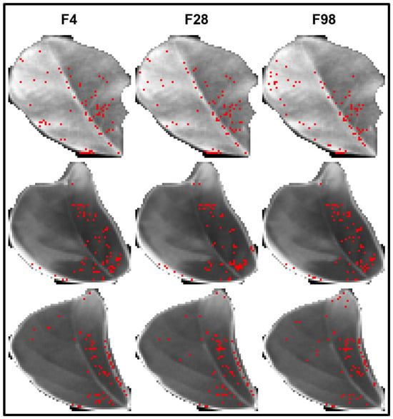
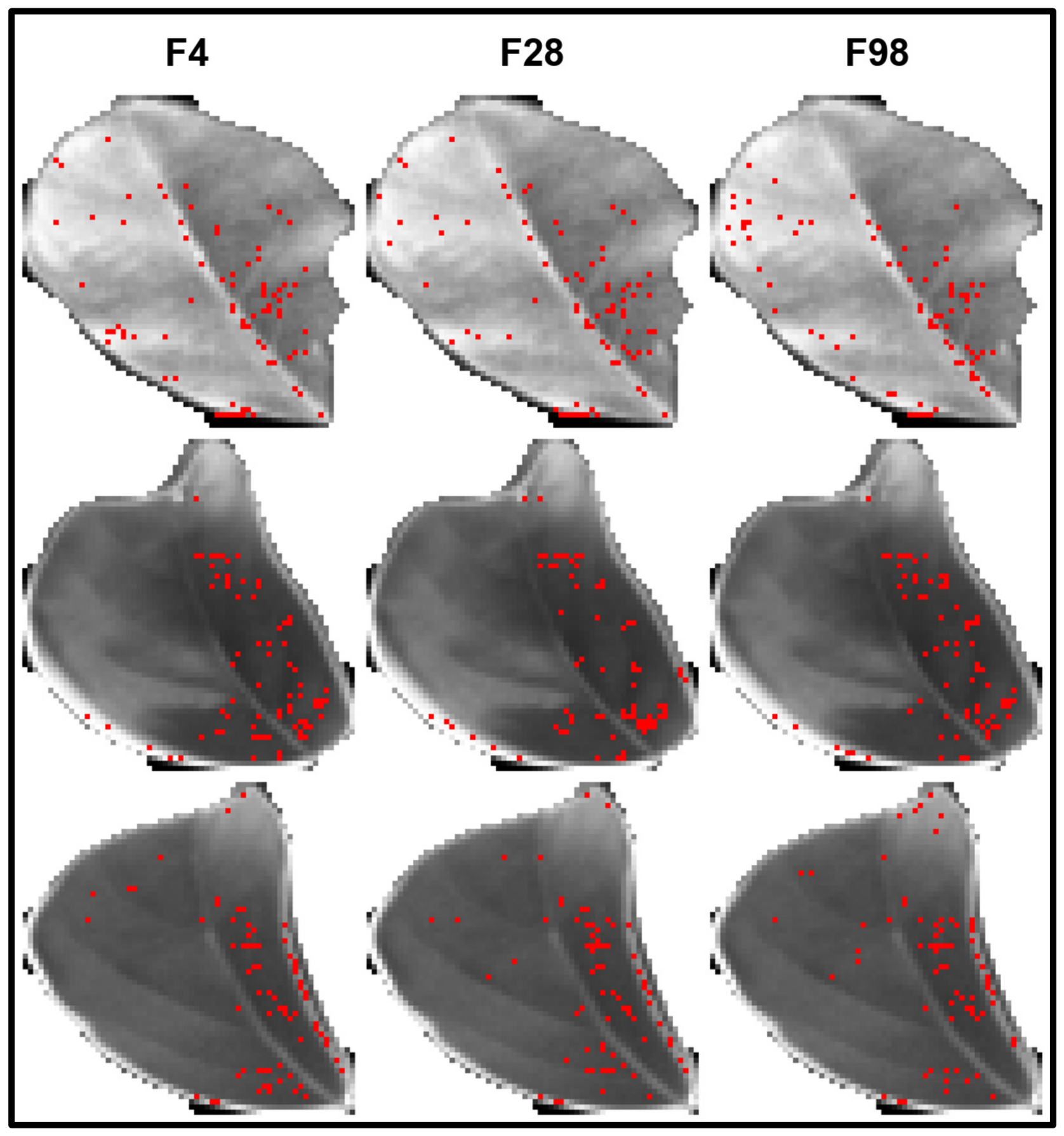
where x is a data instance, f is a feature, SHAPx(f) is the computed SHAP value of f for x, F is all possible subsets of f, |F| is the size of F, ${\widehat{\mathrm{x}}}_{\mathrm{F}}$ represents the model outcome for x with F, and ${\widehat{\mathrm{x}}}_{\mathrm{F}/\mathrm{f}}$ is the predictive outcome for x with F without f. SHAP values were determined in this work using the SHAP “DeepExplainer” function, which is an improved version of the DeepLIFT method [34], was used to calculate SHAP values. Similar to the Kernel SHAP method, DeepExplainer approximates the conditional expectations of SHAP values using a selection of background samples. SHAP values were calculated on the prediction set to quantify the contribution of each chosen feature. The significance of each feature wavelength in predicting outcomes for the CNN model was then demonstrated using the SHAP values, as seen by beeswarm and bar charts. Moreover, further interpretation of the decision-making process at a more detailed spatial level was made possible by using an IG methodology [35,36]. To visualize spatial contributions, IG was applied directly to the input cubes with respect to selected spatial features. Gradients were integrated over 50 steps using a customized leaf-specific mean-spectrum baseline instead of zero. Absolute pixel-level attributions were used to determine the influential regions, and the top 3% of those within the eroded leaf core (2-pixel disk radius) were visualized. Leaf segmentation was done by using ’Otsu’s thresholding’ algorithm and the threshold was automatically determined from red-edge band. The result of this attribution was shown as a red-dot overlaid on the images. Unlike the 1D-CNN predictor, IG was only utilized in the 3D-CNN feature extraction network. In the spatial feature extraction from the multispectral image cube, Pixel-level attributions of the trained 3D-CNN spatial features were computed with IG to identify the spatially influential regions. The embedding vector from the 3D-CNN is sent to the 1D-CNN, which has no spatial dimension, so there is no practical way to implement the IG method. IG attributions are shown as sparse point markers (top 3% of pixels) rather than continuous heatmaps, in which highly impactful (and conspicuous) pixels appear as stand out individual colored points on the image. The most important spatial positions for 3D-CNN spatial feature learning are marked by these dots. The IG identifies and highlights the important regions using gradient-based attribution, which results in a less comprehensive and interpretable spatial significance representation. This dot-based visualization is intended to complement the SHAP-based visualization and spectral analysis, and gives a clearer picture of the effect of certain regional pixel areas, which are not necessarily large, on the regression results and therefore the behavior of the model. SHAP DeepExplainer and IG, when combined, provide a dual-explainability approach to ensure methodologically consistent transparency throughout the spectral and spatial parts of the fusion pipeline.

2.9. Spatial Visualization

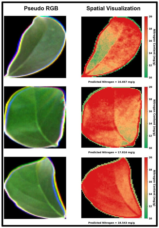
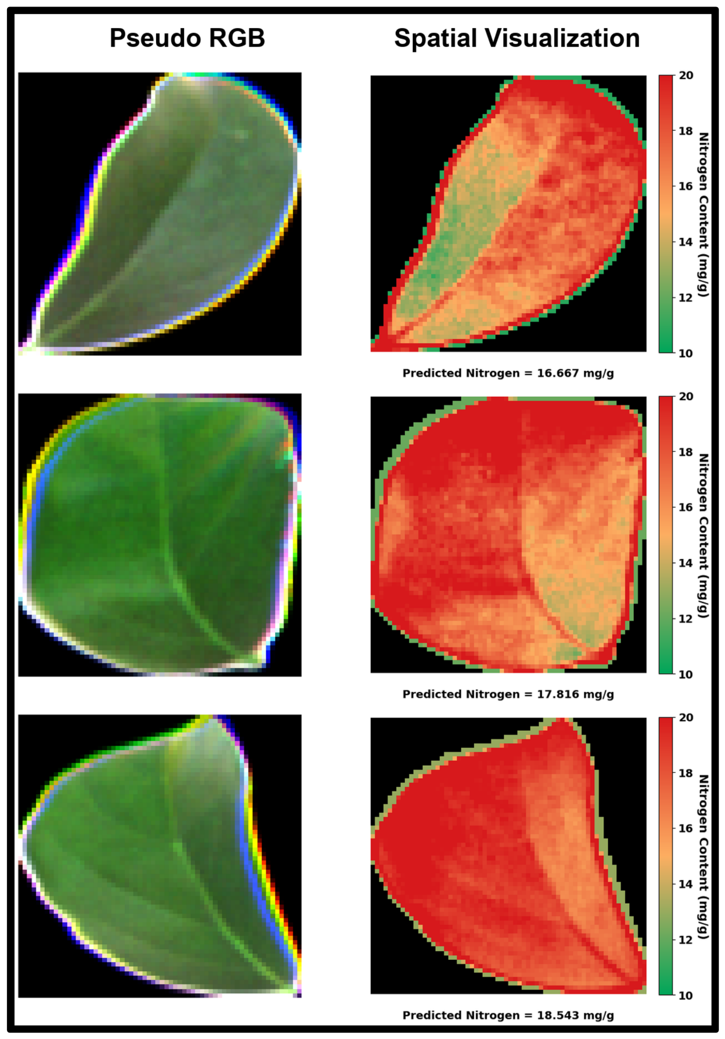
To illustrate the intra-leaf distribution of nitrogen, a pseudo-RGB image was created by combining the red, green, and blue bands of each five-band cube (2nd to 98th percentile stretch, gamma 0.9). To create a leaf mask, the mean of the pseudo-RGB channels was thresholded at 0.08, then binary holes were filled and opened with a 2 × 2 structuring element. To create the mask, each pixel’s MicaSense RedEdge reflectance was centered on the leaf median, split by half of the difference between its 95th and 5th percentiles, and clipped to a range of −1 to 1. Every pixel then has a normalized spatial variation value. This number was multiplied by 6.0 mg/g of display amplitude, which was chosen for visual contrast, and added to the leaf-level nitrogen value (predicted). The map was then shifted by a constant so that its mean matched the leaf-level value before clipping. Values were trimmed to 10–20 mg/g and shown in a green-to-red colormap for cross-leaf comparisons. Individual pixels were not subjected to 1D-CNN, and no pixel-level reference measurements were taken.

2.10. Computational Environment

The “Anaconda” distribution (conda 25.5.1, Anaconda Inc., Austin, TX, USA; https://docs.anaconda.com/) with python 3.10.19 was used to do the calculations in this study. The “shap” module (version 0.49.1) was used to calculate the SHAP values. PyTorch (2.11.0, Meta Platforms, Menlo Park, CA, USA) was used to carry out the Bayesian optimization. A personal computer equipped with a 3.00 GHz Intel(R) CoreTM i9-13900K CPU, NVIDIA GeForce RTX 4090 GPU, and 64 GB of RAM was used for all computations.

3. Results and Discussion

3.1. Spectral Characteristics and Preprocessing

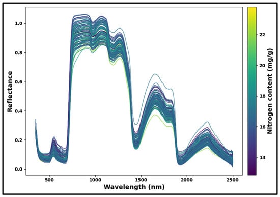
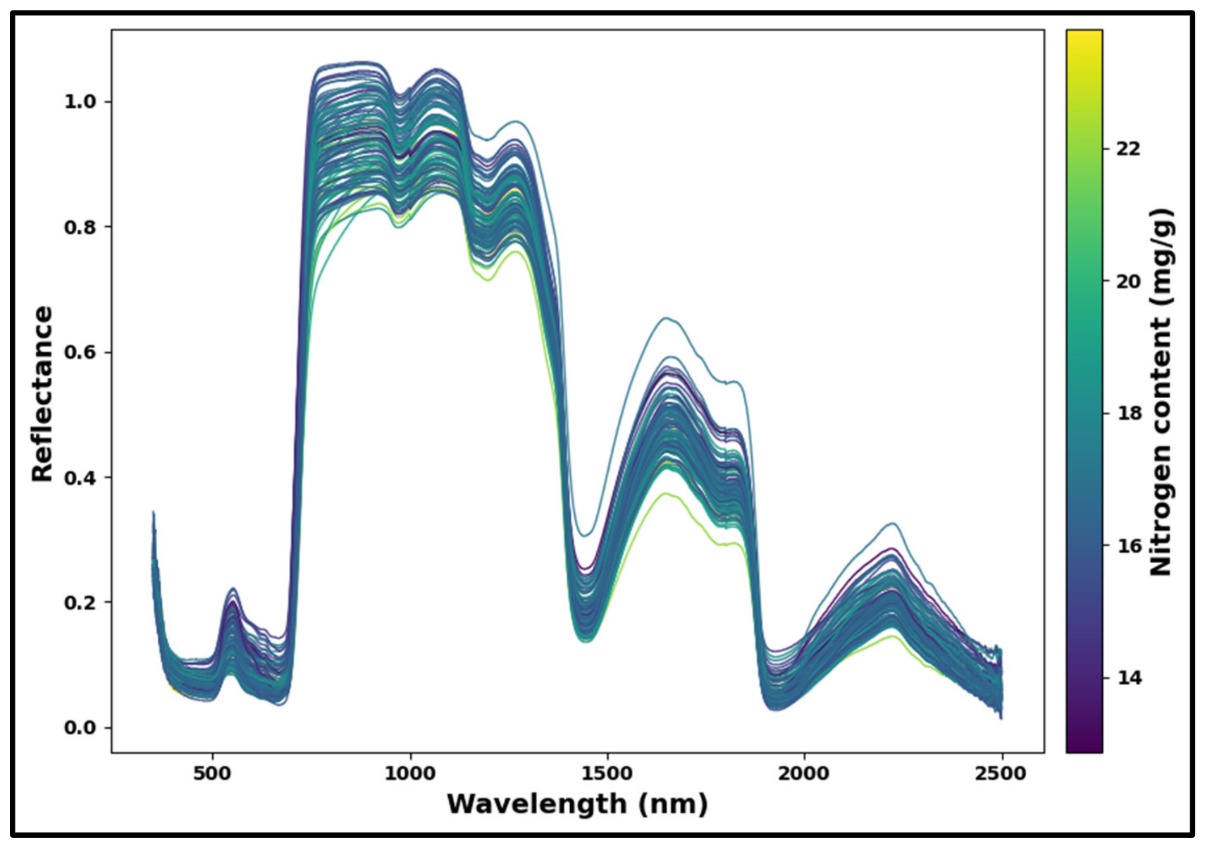
The raw reflectance spectra of Avocado leaves recorded in the 350–2500 nm wavelength range are shown in (Figure 4). The color bar represents the measured nitrogen content (mg/g).

Figure 4. Visualization of original spectra of 104 samples.

Higher-nitrogen samples often exhibit decreased reflectance in the visible area and a red-edge inflection moved toward longer wavelengths, whereas lower-nitrogen samples exhibit the reverse pattern, as illustrated by the color gradient in (Figure 4). This illustrates a clear physical connection: as nitrogen is a structural element of chlorophyll, a larger nitrogen concentration often results in more chlorophyll, more absorption in the blue and red bands, and a red-edge shift to longer wavelengths as the chlorophyll absorption feature widens [37]. Higher nitrogen samples also typically exhibit deeper absorption in the SWIR at the N–H/amide bands, which is consistent with nitrogen being mostly stored in leaf proteins [38].

For leaf reflectance in the visible range (350–750 nm), the amount of pigment absorption is the most important factor [39]. Reflectance is also very low in the blue region (around 400–450 nm) where both chlorophyll a and b, along with accessory pigments such as carotenoids and xanthophylls, have high absorption in order to be able to harvest light for photosynthesis [40]. Reflectance gradually increases until the green region (about 500–580 nm), where a moderate peak is apparent, after declining sharply in the blue region (about 400–450 nm). There is a strong reflectance minimum around 650–680 nm due to the combined absorption of chlorophyll a near 665 nm and chlorophyll b near 652 nm which are the wavelengths corresponding to the Qy electron transition bands [41]. One of the most notable features of the reflectance spectrum is a moderate reflectance peak in the green (500–580 nm) due to the fact that there is no strong absorption of either chlorophyll a or b in this spectral window, leading to a local maximum that provides the characteristic green color of healthy leaves [42].

There is a dramatic and diagnostically significant rise in reflectance between about 700 and 750 nm that is known as the red-edge. This transition is caused by a rapid decrease in the refractive index at the cell wall-intercellular air space interfaces of the leaf mesophyll, and occurs at the border between the strong chlorophyll absorption characteristic of the red wavelengths and the high internal scattering that dominates in the NIR [42,43]. The red-edge region (680–760 nm) is one of the most consistent spectral characteristics of vegetation that correlates with leaf nitrogen and chlorophyll status, as the increase in chlorophyll concentration results in a broadening of the chlorophyll absorption feature which causes the red-edge inflection point to shift towards longer wavelengths [43].

The reflectance values are fairly high and constant in the NIR region (750–1300 nm). In this area, the leaf color components are effective in transmitting radiation, and reflectance is determined by a number of light scatterings at the inner cell wall and intercellular air space surfaces of the spongy and palisade mesophyll layers [42]. NIR reflectance is thus closely related to internal leaf anatomy (intercellular air space volume and mesophyll cell surface area exposed to intercellular air space) instead of biochemical composition [44]. Small fluctuations in this NIR plateau could be due to small differences in leaf thickness, cell packing density and tissue hydration. The SWIR region (1300–2500 nm) contains several prominent absorption features which are due to vibrational modes of chemical bonds in the constituents of the leaves. The two most prominent absorption features, at around 1400 nm and 1900 nm, are predominantly related to the moisture content in the leaf [45]. The feature at 1400 nm is the first overtone of the O–H stretching vibration of water molecules, while the absorption near 1900 nm is due to a combination of the O–H stretching and the H–O–H bending vibrations [46]. These bands, which are dominated by water, increase systematically with decreasing water content of leaves and are thus suitable indicators of leaf water content and water stress [21]. The C–H, N–H and C–O vibrational overtones and combination bands of dry matter constituents such as cellulose, lignin, starch and proteins are responsible for another broad absorption band in the 2200 to 2300 nm region [47]. In particular, the 2100–2180 nm spectral range is correlated with protein content by nitrogen-hydrogen (N–H) bond stretching and combination modes, and the 2280–2300 nm spectral range is correlated with cellulose and lignin content, via C–H and C–O–C combination vibrations [46]. In addition to the indirect relationship with foliar nitrogen content, through the chlorophyll effect, the SWIR region offers a direct biochemical relationship with the foliar nitrogen content, as nitrogen is mainly stored in proteins and amino acids, each of which has amide bonds with N–H absorption features across the SWIR domain [48,49]. Considering overall spectral range, the coverage from 350–2500 nm provides full information about the structural characteristics and metabolic composition of avocado leaves, thus enabling accurate prediction of leaf nitrogen.

3.2. Response Attribute Characteristics

Table 2 shows the descriptive statistics of the nitrogen content of avocado leaves for both calibration and prediction sets. The nitrogen content of all 104 samples ranged from 12.87 to 23.80 mg/g, with an overall mean of 17.25 ± 2.01 mg/g (mean ± standard deviation, SD).

Table 2. Statistics of response attributes for entire set, calibration and prediction sample sets.

Content	Entire Set (n = 104)		Calibration Set (n = 83)		Prediction Set (n = 21)
	Mean ± SD	Range	Mean ± SD	Range	Mean ± SD	Range
Nitrogen (mg/g)	17.25 ± 2.01	12.87–23.80	17.22 ± 2.06	12.87–23.80	17.34 ± 1.83	14.20–21.60

The mean values of the calibration set (17.22 ± 2.06 mg/g) and prediction set (17.34 ± 1.83 mg/g) were comparable, and Levene’s test for equality of variances between the two sets yielded W = 0.294, p = 0.589. The ranges of 12.87–23.80 and 14.20–21.60 mg/g give a well-balanced and representative split of the dataset for KS partitioning. The KS algorithm assigns the most spectrally extreme samples to calibration in order to capture the entire range of variability, leaving more centrally distributed samples for prediction. This is intended to result in a narrower range and lower standard deviations of the prediction set. Because the most extreme nitrogen values are excluded from the prediction set, the given prediction statistics mostly represent interpolation performance rather than extrapolation to extreme values, which is a known trade-off of KS partitioning, particularly for small datasets. For both sets, the nitrogen values are distributed evenly, indicating that the calibration model will be confronted with the entire range of nitrogen variability found in the data, necessary for building strong and generalizable models [25].

3.3. Optimization and Calibration of Spectral Models

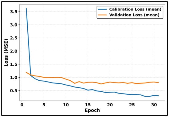
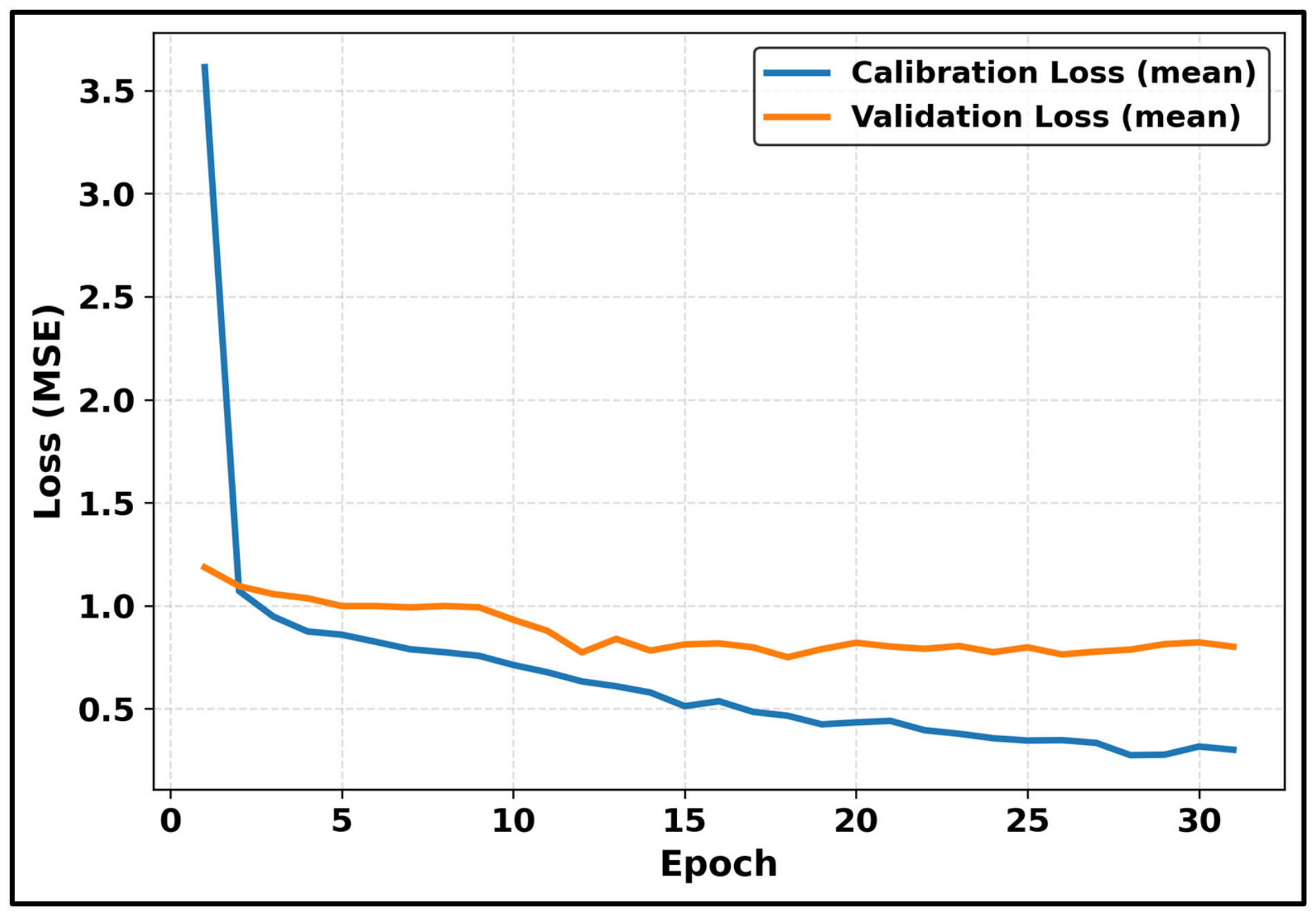
The PLSR and 1D-CNN models are trained on the spectral-only and fused datasets, and their performance is evaluated using calibration and prediction metrics. The loss value during CNN model calibration and validation based on the fusion dataset are illustrated in (Figure 5). The mean calibration and validation losses reduced substantially in the first few epochs, indicating that the model quickly learned the most relevant spectral properties. The curves continued to converge and settle into a stable performance during the 35 epochs, with minor oscillations and no major overfitting. The performance metrics of the PLSR and 1D-CNN are summarized in Table 3 (spectral-only dataset) and Table 4 (fused dataset).

Figure 5. Loss curve of 1D-CNN trained on fusion data.

Table 3. Performance comparison (Mean ± SD) of PLSR and 1D-CNN models trained on spectral data only using 5-fold cross-validation.

Model	Hyperparameters	Trainable Parameters	Calibration R2	Calibration RMSE (mg/g)	Prediction R2	Prediction RMSE (mg/g)	RPD
PLSR	LV: 4	-	0.69 ± 0.06	1.12 ± 0.17	0.55 ± 0.17	1.17 ± 0.21	1.55 ± 0.26
1D-CNN	Conv1D: (48, k = 3), (32, k = 3), Dense: 128, Dropout: (0.4, 0.6, 0.4), LR: 1 × 10−4, Weight Decay: 3.33 × 10−5	2.2M	0.65 ± 0.12	1.18 ± 0.28	0.63 ± 0.08	1.07 ± 0.13	1.68 ± 0.23

Table 4. Performance comparison (Mean ± SD) of all models trained on the fused dataset (spectral reflectance + 3D-CNN spatial features) using 5-fold cross-validation.

Model	Hyperparameters	Trainable Parameters	Calibration R2	Calibration RMSE (mg/g)	Prediction R2	Prediction RMSE (mg/g)	RPD
Data Fusion PLSR	LV: 3	-	0.74 ± 0.09	1.02 ± 0.25	0.57 ± 0.13	1.15 ± 0.20	1.59 ± 0.36
Weighted Fusion PLSR	LV: 5	-	0.59 ± 0.07	1.29 ± 0.13	0.48 ± 0.14	1.26 ± 0.18	1.43 ± 0.22
Data Fusion 1D-CNN	Conv1D: (64, k = 3), (32, k = 3), Dense: 64, Dropout: (0.3, 0.5, 0.4), LR: 1.75 × 10−3, Weight Decay: 1.80 × 10−3	1.6M	0.81 ± 0.07	0.86 ± 0.21	0.73 ± 0.04	0.92 ± 0.08	1.95 ± 0.19
Weighted Fusion 1D-CNN	Conv1D: (16, k = 5), (32, k = 3), Dense: 96, Dropout: (0.4, 0.6, 0.4), LR: 3.5 × 10−4, Weight Decay: 2.0 × 10−3	1.7M	0.68 ± 0.20	1.11 ± 0.38	0.62 ± 0.11	1.08 ± 0.16	1.68 ± 0.26
Attention Fusion 1D-CNN	Conv1D: (48, k = 3), (128, k = 3), Dense: 64, Dropout: (0.3, 0.6, 0.4), LR: 3.3 × 10−4, Weight Decay: 9.37 × 10−5	4.4M	0.73 ± 0.08	1.05 ± 0.19	0.63 ± 0.08	1.07 ± 0.12	1.68 ± 0.17

LV: Latent Variable; Conv1D: (filters, kernel size k); LR: learning rate. Dropout values are listed for the three dropout layers in order.

The advantage of deep learning over linear chemometrics in capturing nonlinear spectral-chemical relationships is reflected by the better performance of 1D-CNN compared to PLSR for the spectral-only models, with a prediction R² of 0.63 and prediction RMSE of 1.07 mg/g (RPD = 1.68), as shown in Table 3.

The model performance was seen to be consistently better with the fusion of 3D-CNN extracted spatial features for CNN based models, as presented in Table 4. The Data Fusion PLSR achieved a prediction R² of 0.57 and prediction RMSE of 1.15 mg/g (RPD = 1.59), compared to R² = 0.55 for spectral-only PLSR. More notably, the Data Fusion 1D-CNN delivered the highest numerical performance, with a calibration R² of 0.81, prediction R² of 0.73, and RPD of 1.95. An RPD of 1.5–2.0 suggests rough screening capabilities rather than exact quantitative prediction, but values ranging from 2.0 to 2.5 permit approximate quantitative evaluation [50]. As a result, the RPD of 1.95 achieved by the Data Fusion 1D-CNN indicates that the suggested framework is suitable for preliminary screening of leaf nitrogen status, albeit its quantitative prediction capability remains limited. Additionally, the corresponding model-wise calibration and prediction parameters, including bias, slope, intercept, and their associated confidence intervals are also reported in Supplementary Information, Tables S1 and S2. Furthermore, multiple random seeds were used to train all of the CNN-based models, which consistently showed promising predictive results (Supplementary Information, Table S3).

The fusion-based models validated that the spatial texture information contained in the multispectral image cubes contains complementary signals that complement the estimation of nitrogen content by spectral reflectance. Overall, the 1D-CNN model performed numerically better in terms of prediction accuracy compared to the model PLSR. This aligns with the ability of CNNs to model complex nonlinear spectral-biochemical relationships [13]. In a fusion-based study, Guo et al. [51] also found benefits from fusing on avocado leaves. Their fusion incorporated vegetation indices with wavelengths picked by Competitive Adaptive Reweighted Sampling (CARS) from the same point spectra, both at the feature and algorithm levels (stacking, voting, bagging). Nitrogen was predicted with a prediction R² of only 0.60. Instead, the present fusion incorporates spatial characteristics from multispectral cubes, directly targets nitrogen (prediction R² = 0.73), and is explained using SHAP and IG.

The weighted and attention-based fusion techniques showed predictive potential in the current experimental setup. The calibration R² value of the Weighted Fusion PLSR was 0.59, while the prediction R² value was 0.48, with an RPD value of 1.43. Similarly, the Weighted Fusion 1D-CNN had a prediction R² of 0.62 and RPD of 1.68, which was less than the Data Fusion 1D-CNN. This is probably because of the static weighting scheme (Spectral = 0.7, Spatial = 0.3), which is unable to adapt to the sample-level variability and can result in sub-optimal or noisy fused representation when the fixed weights are not optimized for each sample. Theoretically, the attention fusion 1D-CNN could learn dynamic cross-modal weighting, but it may have been difficult for it to learn meaningful attention patterns due to limited training data, leading to numerically lower predictive performance compared with the Data Fusion 1D-CNN (prediction R² = 0.63, RPD = 1.68). The results demonstrate that simple concatenation-based data fusion outperforms a weighted fusion and attention-based fusion, which shows that simpler architectures are more robust when the calibration dataset is small. This aligns with the more general problem that training complicated architectures from scratch usually necessitates huge labeled datasets, making simpler or transfer-learning-based methods more appropriate in situations when data availability is constrained [52]. However, simple concatenation produced promising results; statistical analyzes were also performed to measure differences in model performance and the robustness of the results. Weighted Fusion PLSR had the lowest numerical performance (prediction R² = 0.48, RMSE = 1.26), whereas Data Fusion 1D-CNN had the best (prediction R² = 0.73, RMSE = 0.92). Bootstrap and Fisher-Z 95% confidence ranges for prediction R² overlapped across all model pairs (Supplementary Table S1). Prediction biases were minimal (≤0.16 mg/g), with sub-unity slopes across all models (Supplementary Table S2). However, no model pairs indicated statistically significant differences in the Holm-Bonferroni adjusted pairwise comparisons (all p > 0.05). As a result, despite numerical differences, no significant difference was found across the seven models, and the numerical advantage of Data Fusion 1D-CNN is regarded suggestive rather than statistically established given the sample size.

The portable TYS-4N reference analyzer’s ±5% measurement error creates a ‘noise ceiling’, limiting the models prediction R² and RMSE. Future investigations should use established laboratory chemistry procedures (Kjeldahl or Dumas) to create a more robust baseline. Additionally, the prediction set had a smaller nitrogen range than the calibration set. As a result, the reported metrics are limited to interpolation performance. This limitation shows that the models have not been tested across a wider range of nitrogen concentrations. Therefore, future studies will concentrate on increasing the concentration range for both calibration and prediction to include extreme nitrogen values. Beyond these limitations, the dataset was collected from a single cultivar and sampling time; therefore, its robustness across different cultivars and seasons remains untested. Another drawback of this study is that there is no metadata available for trees, so grouped cross-validation is not possible. Future studies will employ group-aware cross-validation and test model generalizability with an independent test set collected from completely different trees, to evaluate performance in new trees. Finally, scaling to field photography is another problem. Specifically, the 1D-CNN was trained on 2151 spectrometer bands, but the maps employed five MicaSense bands. Therefore, unmanned aerial vehicle (UAV) mapping will require band resampling and cross-instrument calibration. Consequently, the current maps are qualitative at the leaf scale.

3.4. Explanation of the CNN Model Using DeepExplainer

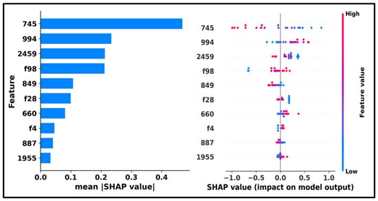
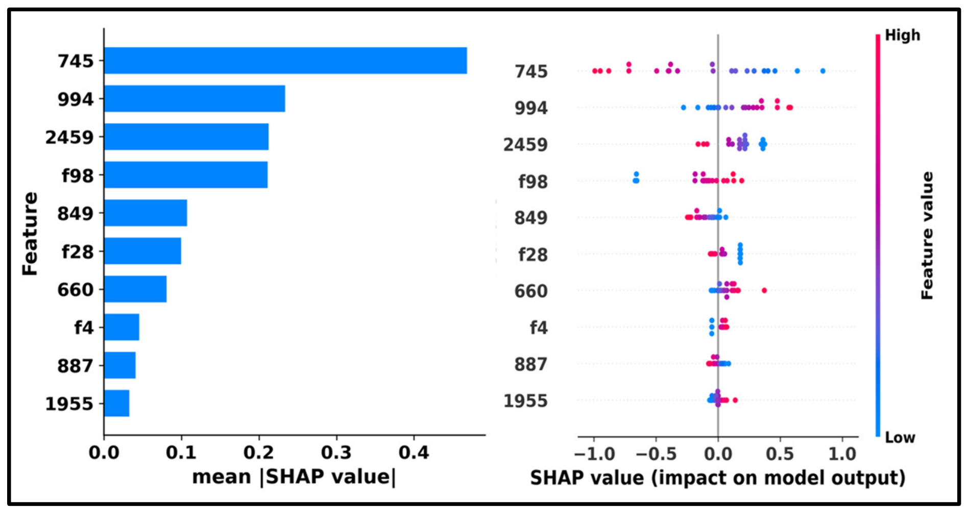
Since the best-performing model was found to be the Data Fusion 1D-CNN, its predictions were assessed using SHAP. (Figure 6) shows the summary plots and SHAP feature importance bar for the top-performing Data Fusion 1D-CNN model.

Figure 6. The summary (right) and SHAP feature importance bar (left) graphs for the CNN model used to estimate the avocado’s nitrogen content. The Y-axis displays wavelengths ranked by significance, while the X-axis displays SHAP values that indicate each feature’s influence on the model output.

The summary plot displays the distribution and direction of feature contributions across all samples, while the bar plot displays the global significance of the top 10 features based on the mean absolute SHAP values. The most dominant features are 745 nm, 994 nm, 2459 nm, 849 nm, 660 nm, 887 nm and 1955 nm, and the spatial features f98, f28, and f4 extracted from the multispectral image cubes, as depicted in the bar plot. The stability of the SHAP feature rankings was further assessed using bootstrap resampling. Results showed a mean Spearman correlation coefficient of 0.87 ± 0.08 and a top-3 Jaccard similarity of 0.79 ± 0.25, demonstrating consistent feature relevance across resampling. Notably, the 745 nm feature consistently ranked first across all resamples, indicating its dominant contribution to nitrogen prediction. The dominance of the 745 nm feature, located in the red-edge region, is particularly relevant because this region is sensitive to plant physiological conditions, including chlorophyll content.

Previous studies have also reported that specific spectral regions such as the red-edge, NIR, and SWIR are strongly associated with crop nitrogen status. The red-edge region around 700 nm has been widely identified as highly sensitive to leaf nitrogen and chlorophyll concentration in vegetation [53]. According to a different study, the most effective and consistent location for determining crop nitrogen status is the red-edge position (680–760 nm) [54]. The red-edge region, which is the unique transition area between the high NIR reflectance (near 760 nm) by leaf internal structural characteristics and the strong red-light absorption (near 680 nm) by leaf pigments, contains a wealth of vegetation absorption and reflection information and is crucial for estimating the canopy’s chlorophyll and nitrogen status [55]. The visible bands, which are centered at 660 nm and 640 nm, respectively, are associated with absorption by chlorophyll a and b [56]. This connection relates to the significant impact of nitrogen on the synthesis and operation of chlorophyll [57]. Spectral bands in the red-to-red-edge region show strong sensitivity to nitrogen content in plants. In particular, wavelengths around 649 nm, 659 nm, and 685 nm exhibit the highest correlation with leaf nitrogen content [58]. In addition, spectral bands in the NIR region (700–1000 nm) are closely related to canopy structure and biomass, which indirectly influence nitrogen estimation [59]. It has been discovered that there is a strong correlation between N concentration and reflectance spectra in the SWIR spectrum region (1100–2500 nm). Protein absorption characteristics, the initial overtone, and the N–H stretch are all directly correlated with reflectance in this area [60]. The SWIR region (1200–2500 nm) is important for nitrogen estimation because absorption features, particularly around 1510 nm, are directly associated with nitrogen and protein content in plants. Proteins and amino acids, which include amide bonds with absorption bands in the SWIR range (1550–1750 nm), are the main sources of nitrogen in fresh leaves [49]. The main absorption features associated with nitrogen and proteins, which are mostly found in the SWIR area between 1000 and 2400 nm, are not included in this range, despite the fact that it captures chlorophyll-related features and canopy structural impacts. In particular, direct biological absorption associated with proteins and nitrogen molecules is reflected by N–H stretching and combination bands about 1020, 1510, 1730, 1980, 2060, 2130, 2180, 2240, and 2300 nm [61].

The SHAP summary plot shows wider, more asymmetric SHAP value distributions, indicating the model’s ability to capture complex nonlinear relationships in the data. Spatial features f98, f28 and f4, extracted from the 3D-CNN feature extraction of multispectral image cubes, also rank in the top contributors, highlighting the complementary signals in addition to the spectral reflectance that can be obtained from leaves. Although the spectral wavelengths and deep spatial features (f98, f28, f4) are derived from the same fused input vector and thus share a common SHAP scale, their direct ranking should be interpreted with caution because spatial features are compressed nonlinear embeddings that aggregate information across an entire image cube, while individual wavelengths are physically interpretable but derived from a highly autocorrelated 2151-band continuum. A higher SHAP value for a spatial feature indicates greater net predictive weight within the fused representation rather than intrinsically greater physiological importance than the spectral region it is compared against because this granularity difference can dilute per-wavelength SHAP contributions relative to spatial embeddings.

The integration of spatial and spectral features numerically improves nitrogen estimation accuracy compared to using spectral information alone. Leaf venation structure provides important spatial information that contributes to nitrogen prediction [11]. Reflectance is influenced not only by biochemical properties but also by leaf structure and internal organization. And although nitrogen estimation relies on spectral reflectance, the measured signal is strongly influenced by canopy structure, indicating that spatial characteristics also play a critical role [62]. The majority of conventional deep learning techniques for MSI extract spatial or spectral data separately. It is challenging to completely utilize all of the information from an MSI cube at once because these two are extracted independently. Overall, the identified wavelengths in red, red-edge, and SWIR bands are in good accordance with the well-known spectral features of nitrogen-sensitive vegetation found in the study [58,61], which confirms the biological relevance of the model learned representations.

IG attributions for the 3D-CNN feature extractor were computed to identify the leaf regions influencing the spatial features. The IG visualization for the 3D-CNN spatial features f4, f28, and f98 is presented in Figure 7.

Figure 7. Integrated Gradients visualization highlighting important pixels from CNN-extracted features (f4, f28, f98) used in spectroscopic fusion. Red dots mark the top 3% of pixels with the highest absolute attribution within the leaf core.

Figure 7 shows the IG visualization for the 3D-CNN spatial features f98, f28, and f4. The activated pixel regions demonstrate that the 3D-CNN captures spatially meaningful patterns related to leaf edges, venation structure, and areas of textural variation. By confirming that the spectral–spatial fusion framework captures both biochemically relevant wavelengths and structurally informative leaf regions, these dot-based attribution patterns support the SHAP findings and strengthen the developed model’s biological validity and interpretability.

3.5. Multispectral Visualization and Nitrogen Prediction Mapping

Figure 8 compares the pseudo-RGB image to the nitrogen distribution map for each leaf. The relative spatial pattern is derived from the MicaSense image’s RedEdge band, while the absolute level is determined by the leaf-level value. Because the map is centered on the leaf-level value, its mean equals that value before clipping, which ensures that the maps match the leaf-level result. This consistency exists by construction but does not validate the spatial pattern.

Figure 8. Visualization of nitrogen content in leaves.

The within-leaf spread is set by the display amplitude (±6.0 mg/g) and was not estimated from the data. The 1D-CNN was trained on 2151 ASD wavelengths (350–2500 nm) and cannot be applied directly to the five MicaSense bands, hence the maps do not represent independent pixel-level predictions. They provide a qualitative sense of spatial variability that is not apparent in RGB images. Pixel-level prediction will necessitate band resampling, cross-instrument calibration, and pixel-level reference information.

4. Conclusions

This study demonstrates that nitrogen content prediction can be numerically improved by integrating MSI with a feature-level fusion strategy. While PLSR and 1D-CNN models provided rough screening estimates from only spectral reflectance, incorporating spatial–spectral features extracted with a 3D-CNN yielded marginally improved predictive performance. The findings suggest that structural information within multispectral cubes contributes complementary signals beyond those captured by spectra alone. The integration of XAI further enhanced model transparency by identifying influential wavelengths and fused features driving nitrogen estimation. This added interpretability supports more informed wavelength selection and strengthens the practical applicability of machine learning in multispectral nitrogen assessment. Simple concatenation-based data fusion had the highest numerical accuracy across all assessed fusion procedures. However, the differences were not statistically significant when compared to the other models. Weighted fusion PLSR did worse than spectral-only PLSR. The weighted fusion 1D-CNN and attention-based fusion 1D-CNN produced prediction R² values of 0.62 and 0.63, respectively, which were comparable to the spectral-only 1D-CNN (0.63). Only simple concatenation demonstrated a numerical advantage over spectral-only models. The results show that, in limited-data scenarios, simplicity in architectural design may be preferable to a more complex adaptive design. However, the limited amount of data (only 104 samples, 1 cultivar, 1 region) restricts the generalizability of the model and may have restricted the performance of attention-based fusion. Future research should include additional cultivars, seasons, and locations, as well as independent test sets from various trees. When labeled data is limited, self-supervised learning and transformer-based architectures can help with fusion. The nitrogen maps in this study are qualitative, therefore quantitative pixel-level mapping will necessitate spectral resampling and cross-instrument calibration. Validating the XAI outcomes against plant physiological information might strengthen their interpretation.

References

- Pérez, V.; Larranaga, N.; Alcaraz, M.L.; Hormaza, J.I. Genotyping and diversity analysis of local avocado landraces in La Palma, Canary Islands. Front. Plant Sci. 2025, 16, 1572870. [Google Scholar] [CrossRef] [Scilit] [PubMed]
- Guan, C.; Zhang, D.; Chu, C. Interplay of light and nitrogen for plant growth and development. Crop J. 2025, 13, 641–655. [Google Scholar] [CrossRef] [Scilit]
- Li, D.; Zhang, P.; Chen, T.; Qin, W. Recent Development and Challenges in Spectroscopy and Machine Vision Technologies for Crop Nitrogen Diagnosis: A Review. Remote Sens. 2020, 12, 2578. [Google Scholar] [CrossRef] [Scilit]
- Rehman, T.U.; Mahmud, M.; Chang, Y.K.; Jin, J.; Shin, J. Current and future applications of statistical machine learning algorithms for agricultural machine vision systems. Comput. Electron. Agric. 2019, 156, 585–605. [Google Scholar] [CrossRef] [Scilit]
- Zhang, Q.; Luan, R.; Wang, M.; Zhang, J.; Yu, F.; Ping, Y.; Qiu, L. Research Progress of Spectral Imaging Techniques in Plant Phenotype Studies. Plants 2024, 13, 3088. [Google Scholar] [CrossRef] [Scilit] [PubMed]
- Rahman, M.; Busby, S.; Ru, S.; Hanif, S.; Sanz-Saez, A.; Zheng, J.; Rehman, T.U. Transformer-Based hyperspectral image analysis for phenotyping drought tolerance in blueberries. Comput. Electron. Agric. 2025, 228, 109684. [Google Scholar] [CrossRef] [Scilit]
- Berger, K.; Verrelst, J.; Féret, J.B.; Wang, Z.; Wocher, M.; Strathmann, M.; Danner, M.; Mauser, W.; Hank, T. Crop nitrogen monitoring: Recent progress and principal developments in the context of imaging spectroscopy missions. Remote Sens. Environ. 2020, 242, 111758. [Google Scholar] [CrossRef] [Scilit] [PubMed]
- Hossen, M.A.; Diwakar, P.K.; Ragi, S. Total nitrogen estimation in agricultural soils via aerial multispectral imaging and LIBS. Sci. Rep. 2021, 11, 12693. [Google Scholar] [CrossRef] [Scilit] [PubMed]
- Burnett, A.C.; Anderson, J.; Davidson, K.J.; Ely, K.S.; Lamour, J.; Li, Q.; Morrison, B.D.; Yang, D.; Rogers, A.; Serbin, S.P. A best-practice guide to predicting plant traits from leaf-level hyperspectral data using partial least squares regression. J. Exp. Bot. 2021, 72, 6175–6189. [Google Scholar] [CrossRef] [Scilit] [PubMed]
- Okyere, F.G.; Cudjoe, D.; Sadeghi-Tehran, P.; Virlet, N.; Riche, A.B.; Castle, M.; Greche, L.; Simms, D.; Mhada, M.; Mohareb, F.; et al. Modeling the spatial-spectral characteristics of plants for nutrient status identification using hyperspectral data and deep learning methods. Front. Plant Sci. 2023, 14, 1209500. [Google Scholar] [CrossRef] [Scilit] [PubMed]
- Song, Z.; Wei, X.; Zhang, J.; Chen, Z.; Jin, J. Spatial-spectral feature mining in hyperspectral corn leaf venation structure and its application in nitrogen content estimation. Comput. Electron. Agric. 2024, 227, 109495. [Google Scholar] [CrossRef] [Scilit]
- Zhang, X.; Xu, J.; Yang, J.; Chen, L.; Zhou, H.; Liu, X.; Li, H.; Lin, T.; Ying, Y. Understanding the learning mechanism of convolutional neural networks in spectral analysis. Anal. Chim. Acta 2020, 1119, 41–51. [Google Scholar] [CrossRef] [Scilit] [PubMed]
- Passos, D.; Mishra, P. Deep Tutti Frutti: Exploring CNN architectures for dry matter prediction in fruit from multi-fruit near-infrared spectra. Chemom. Intell. Lab. Syst. 2023, 243, 105023. [Google Scholar] [CrossRef] [Scilit]
- Ahmad, M.; Khan, A.M.; Mazzara, M.; Distefano, S.; Ali, M.; Sarfraz, M.S. A Fast 3D CNN for Hyperspectral Image Classification. IEEE Geosci. Remote Sens. Lett. 2020, 19, 5502205. [Google Scholar] [CrossRef] [Scilit]
- Li, Y.; Zhang, L.; Chen, L.; Ma, Y. Superpixel guided spectral-spatial feature extraction and weighted feature fusion for hyperspectral image classification with limited training samples. Sci. Rep. 2025, 15, 3473. [Google Scholar] [CrossRef] [Scilit] [PubMed]
- Ahmed, T.; Wijewardane, N.K.; Lu, Y.; Jones, D.S.; Kudenov, M.; Williams, C.; Villordon, A.; Kamruzzaman, M. Advancing sweetpotato quality assessment with hyperspectral imaging and explainable artificial intelligence. Comput. Electron. Agric. 2024, 220, 108855. [Google Scholar] [CrossRef] [Scilit]
- Sundararajan, M.; Taly, A.; Yan, Q. Axiomatic Attribution for Deep Networks. arXiv 2017, arXiv:1703.01365. [Google Scholar] [CrossRef] [Scilit]
- Zhang, X.; Hu, Y.; Li, X.; Wang, P.; Guo, S.; Wang, L.; Zhang, C.; Ge, X. Estimation of Rice Leaf Nitrogen Content Using UAV-Based Spectral–Texture Fusion Indices (STFIs) and Two-Stage Feature Selection. Remote Sens. 2025, 17, 2499. [Google Scholar] [CrossRef] [Scilit]
- Castaldi, F.; Castrignanò, A.; Casa, R. A data fusion and spatial data analysis approach for the estimation of wheat grain nitrogen uptake from satellite data. Int. J. Remote Sens. 2016, 37, 4317–4336. [Google Scholar] [CrossRef] [Scilit]
- Zhang, J.; Wei, X.; Song, Z.; Chen, Z.; Jin, J. A high-precision spatial and spectral imaging solution for accurate corn nitrogen content level prediction at early vegetative growth stages. Comput. Electron. Agric. 2025, 230, 109940. [Google Scholar] [CrossRef] [Scilit]
- Estrada, J.S.; Demarco, R.; Johnson, C.M.; Zañartu, M.; Fuentes, A.; Auat Cheein, F. A multi-spectral and hyperspectral image dataset for evaluating chemical traits and the water status of avocado, olive and grape through leaf dehydration under laboratory conditions. Sci. Rep. 2025, 15, 2973. [Google Scholar] [CrossRef] [Scilit] [PubMed]
- Estrada, J.S. A Multi-Spectral and Hyperspectral Image Dataset for Evaluating the Health Status of Avocado, Olive and Vineyard [Dataset]. figshare 2024. Available online: https://figshare.com/articles/dataset/_b_A_multi-spectral_and_hyperspectral_image_dataset_for_evaluating_the_health_status_of_avocado_olive_and_vineyard_b_/26950660?file=49034797 (accessed on 31 October 2026).
- Liantoni, F.; Bataona, D.S. Region growing segmentation based on otsu threshold for detection of guava leaf diseases. AIP Conf. Proc. 2026, 3337, 030020. [Google Scholar] [CrossRef] [Scilit]
- Ahmed, M.; Ahmed, M.W.; Kamruzzaman, M. SpectroChat: A windows executable graphical user interface for chemometrics analysis of spectroscopic data. Softw. Impacts 2024, 21, 100698. [Google Scholar] [CrossRef] [Scilit]
- Petrovskaia, A.; Gasanov, M.; Nikitin, A.; Tregubova, P.; Oseledets, I. Maximizing dataset variability in agricultural surveys with spatial sampling based on MaxVol matrix approximation. Precis. Agric. 2025, 26, 9. [Google Scholar] [CrossRef] [Scilit]
- Dwivedi, S.; Mandal, M.; Yadav, S.; Vipparthi, S.K. 3D CNN with Localized Residual Connections for Hyperspectral Image Classification. In Computer Vision and Image Processing; Springer: Singapore, 2020; pp. 354–363. [Google Scholar] [CrossRef] [Scilit]
- Ben Hamida, A.; Benoit, A.; Lambert, P.; Ben Amar, C. 3-D Deep Learning Approach for Remote Sensing Image Classification. IEEE Trans. Geosci. Remote Sens. 2018, 56, 4420–4434. [Google Scholar] [CrossRef] [Scilit]
- Li, Y.; El Habib Daho, M.; Conze, P.H.; Zeghlache, R.; Le Boité, H.; Tadayoni, R.; Cochener, B.; Lamard, M.; Quellec, G. A review of deep learning-based information fusion techniques for multimodal medical image classification. Comput. Biol. Med. 2024, 177, 108635. [Google Scholar] [CrossRef] [Scilit] [PubMed]
- Islam, M.; Khatun, M.; Chyon, M.S.A.; Anzoom, R.; Imtiaz, M.; Iqbal, S.M.H.S.; Azam, S.; Rahim, A.; Ahmed, W.; Ahmed, T. Comparative analysis of explainable machine learning integrated with hyperspectral imaging for early prediction of wheat yield. Talanta 2026, 308, 129955. [Google Scholar] [CrossRef] [Scilit] [PubMed]
- Ahmed, M.; Villordon, A.; Kamruzzaman, M. Hyperspectral imaging and explainable deep-learning for non-destructive quality prediction of sweetpotato. Postharvest Biol. Technol. 2025, 222, 113379. [Google Scholar] [CrossRef] [Scilit]
- Rey, D.; Neuhäuser, M. Wilcoxon-Signed-Rank Test. In International Encyclopedia of Statistical Science; Springer: Berlin/Heidelberg, Germany, 2011; pp. 1658–1659. [Google Scholar] [CrossRef] [Scilit]
- Khatun, M.; Islam, M.; Imtiaz, M.; Ahmed, M.W.; Ahmed, M. Explainable AI-Guided Hyperspectral Feature Selection in Fruit Quality Assessment and Spatial Visualization. J. Food Sci. 2026, 91, e70976. [Google Scholar] [CrossRef] [Scilit] [PubMed]
- Shapley, L.S. 17. A Value for n-Person Games. In Contributions to the Theory of Games (AM-28), Volume II; Princeton University Press: Princeton, NJ, USA, 1953; pp. 307–318. [Google Scholar] [CrossRef] [Scilit]
- Shrikumar, A.; Greenside, P.; Kundaje, A. Learning Important Features Through Propagating Activation Differences [Internet]. 2017. Available online: http://goo.gl/RM8jvH (accessed on 31 October 2026).
- Jia, L.; Zhang, X.; Kong, B.; Hu, J.; Wu, Y.; Liu, S. SREM-Net: A Novel Leaf Disease Classification Model for Field Crops Based on Stylistic and Multiscale Feature Extraction. Agronomy 2025, 16, 58. [Google Scholar] [CrossRef] [Scilit]
- Ahmed, M.T.; Ahmed, M.W.; Kamruzzaman, M. A systematic review of explainable artificial intelligence for spectroscopic agricultural quality assessment. In Computers and Electronics in Agriculture; Elsevier B.V.: Amsterdam, The Netherlands, 2025. [Google Scholar] [CrossRef] [Scilit]
- Wang, S.; Guan, K.; Wang, Z.; Ainsworth, E.A.; Zheng, T.; Townsend, P.A.; Li, K.; Moller, C.; Wu, G.; Jiang, C. Unique contributions of chlorophyll and nitrogen to predict crop photosynthetic capacity from leaf spectroscopy. J. Exp. Bot. 2021, 72, 341–354. [Google Scholar] [CrossRef] [Scilit] [PubMed]
- Raper, T.B.; Varco, J.J. Canopy-scale wavelength and vegetative index sensitivities to cotton growth parameters and nitrogen status. Precis. Agric. 2015, 16, 62–76. [Google Scholar] [CrossRef] [Scilit]
- Ustin, S.L.; Jacquemoud, S. How the Optical Properties of Leaves Modify the Absorption and Scattering of Energy and Enhance Leaf Functionality. In Remote Sensing of Plant Biodiversity; Springer International Publishing: Cham, Switzerland, 2020; pp. 349–384. [Google Scholar] [CrossRef] [Scilit]
- Falcioni, R.; Antunes, W.C.; Demattê, J.A.M.; Nanni, M.R. A Novel Method for Estimating Chlorophyll and Carotenoid Concentrations in Leaves: A Two Hyperspectral Sensor Approach. Sensors 2023, 23, 3843. [Google Scholar] [CrossRef] [Scilit] [PubMed]
- Zahn, C.; Stensitzki, T.; Heyne, K. Femtosecond anisotropy excitation spectroscopy to disentangle the Qx and Qy absorption in chlorophyll a. Chem. Sci. 2022, 13, 12426–12432. [Google Scholar] [CrossRef] [Scilit] [PubMed]
- Xu, K.; Ye, H. Light scattering in stacked mesophyll cells results in similarity characteristic of solar spectral reflectance and transmittance of natural leaves. Sci. Rep. 2023, 13, 4694. [Google Scholar] [CrossRef] [Scilit] [PubMed]
- Neuwirthová, E.; Lhotáková, Z.; Albrechtová, J. The Effect of Leaf Stacking on Leaf Reflectance and Vegetation Indices Measured by Contact Probe during the Season. Sensors 2017, 17, 1202. [Google Scholar] [CrossRef] [Scilit] [PubMed]
- Li, C.; Czyż, E.A.; Halitschke, R.; Baldwin, I.T.; Schaepman, M.E.; Schuman, M.C. Evaluating potential of leaf reflectance spectra to monitor plant genetic variation. Plant Methods 2023, 19, 108. [Google Scholar] [CrossRef] [Scilit] [PubMed]
- Wilson, R.H.; Nadeau, K.P.; Jaworski, F.B.; Tromberg, B.J.; Durkin, A.J. Review of short-wave infrared spectroscopy and imaging methods for biological tissue characterization. J. Biomed. Opt. 2015, 20, 030901. [Google Scholar] [CrossRef] [Scilit] [PubMed]
- Purwadi, I.; Erskine, P.D.; van der Ent, A. Reflectance spectroscopy as a promising tool for ‘sensing’ metals in hyperaccumulator plants. Planta 2023, 258, 41. [Google Scholar] [CrossRef] [Scilit] [PubMed]
- Lippolis, A.; Polo, P.V.; de Sousa, G.; Dechesne, A.; Pouvreau, L.; Trindade, L.M. High-throughput seed quality analysis in faba bean: Leveraging Near-InfraRed spectroscopy (NIRS) data and statistical methods. Food Chem. X 2024, 23, 101583. [Google Scholar] [CrossRef] [Scilit] [PubMed]
- Féret, J.B.; Berger, K.; de Boissieu, F.; Malenovský, Z. PROSPECT-PRO for estimating content of nitrogen-containing leaf proteins and other carbon-based constituents. Remote Sens. Environ. 2021, 252, 112173. [Google Scholar] [CrossRef] [Scilit]
- Wijewardane, N.K.; Zhang, H.; Yang, J.; Schnable, J.C.; Schachtman, D.P.; Ge, Y. A leaf-level spectral library to support high-throughput plant phenotyping: Predictive accuracy and model transfer. J. Exp. Bot. 2023, 74, 4050–4062. [Google Scholar] [CrossRef] [Scilit] [PubMed]
- Saeys, W.; Mouazen, A.M.; Ramon, H. Potential for Onsite and Online Analysis of Pig Manure using Visible and Near Infrared Reflectance Spectroscopy. Biosyst. Eng. 2005, 91, 393–402. [Google Scholar] [CrossRef] [Scilit]
- Guo, Z.; Estrada, J.S.; Guo, X.; Shamshiri, R.R.; Pereyra, M.; Auat Cheein, F. Integrative Nutritional Assessment of Avocado Leaves Using Entropy-Weighted Spectral Indices and Fusion Learning. Computation 2026, 14, 33. [Google Scholar] [CrossRef] [Scilit]
- Mahmud, M.S.; He, L.; Zahid, A.; Heinemann, P.; Choi, D.; Krawczyk, G.; Zhu, H. Detection and infected area segmentation of apple fire blight using image processing and deep transfer learning for site-specific management. Comput. Electron. Agric. 2023, 209, 107862. [Google Scholar] [CrossRef] [Scilit]
- Gitelson, A.A.; Merzlyak, M.N.; Lichtenthaler, H.K. Detection of Red Edge Position and Chlorophyll Content by Reflectance Measurements Near 700 nm. J. Plant Physiol. 1996, 148, 501–508. [Google Scholar] [CrossRef] [Scilit]
- Shiratsuchi, L.; Ferguson, R.; Shanahan, J.; Adamchuk, V.; Rundquist, D.; Marx, D.; Slater, G. Water and Nitrogen Effects on Active Canopy Sensor Vegetation Indices. Agron. J. 2011, 103, 1815–1826. [Google Scholar] [CrossRef] [Scilit]
- Guo, B.B.; Qi, S.L.; Heng, Y.R.; Duan, J.Z.; Zhang, H.Y.; Wu, Y.P.; Feng, W.; Xie, Y.X.; Zhu, Y.J. Remotely assessing leaf N uptake in winter wheat based on canopy hyperspectral red-edge absorption. Eur. J. Agron. 2017, 82, 113–124. [Google Scholar] [CrossRef] [Scilit]
- Curran, P.J.; Dungan, J.L.; Peterson, D.L. Estimating the foliar biochemical concentration of leaves with reflectance spectrometry. Remote Sens. Environ. 2001, 76, 349–359. [Google Scholar] [CrossRef] [Scilit]
- Ferwerda, J.G.; Skidmore, A.K.; Mutanga, O. Nitrogen detection with hyperspectral normalized ratio indices across multiple plant species. Int. J. Remote Sens. 2005, 26, 4083–4095. [Google Scholar] [CrossRef] [Scilit]
- Ma, C.; Zhai, L.; Li, C.; Wang, Y. Hyperspectral Estimation of Nitrogen Content in Different Leaf Positions of Wheat Using Machine Learning Models. Appl. Sci. 2022, 12, 7427. [Google Scholar] [CrossRef] [Scilit]
- Chu, X.; Guo, Y.; He, J.; Yao, X.; Zhu, Y.; Cao, W.; Cheng, T.; Tian, Y. Comparison of Different Hyperspectral Vegetation Indices for Estimating Canopy Leaf Nitrogen Accumulation in Rice. Agron. J. 2014, 106, 1911–1920. [Google Scholar] [CrossRef] [Scilit]
- Fiorio, P.R.; Silva, C.A.A.C.; Rizzo, R.; Demattê, J.A.M.; dos Santos Luciano, A.C.; da Silva, M.A. Prediction of leaf nitrogen in sugarcane (Saccharum spp.) by Vis-NIR-SWIR spectroradiometry. Heliyon 2024, 10, e26819. [Google Scholar] [CrossRef] [Scilit] [PubMed]
- Yu, K.; Belwalkar, A.; Wang, W.; Hu, Y.; Hunegnaw, A.; Nurunnabi, A.; Ruf, T.; Li, F.; Jia, L.; Kooistra, L.; et al. UAV hyperspectral remote sensing for crop nitrogen monitoring: Progress, challenges, and perspectives. Smart Agric. Technol. 2025, 12, 101507. [Google Scholar] [CrossRef] [Scilit]
- Knyazikhin, Y.; Schull, M.A.; Stenberg, P.; Mõttus, M.; Rautiainen, M.; Yang, Y.; Marshak, A.; Carmona, P.L.; Kaufmann, R.K.; Lewis, P.; et al. Hyperspectral remote sensing of foliar nitrogen content. Proc. Natl. Acad. Sci. USA 2013, 110, E185–E192. [Google Scholar] [CrossRef] [Scilit] [PubMed]
Disclaimer/Publisher’s Note: The statements, opinions and data contained in all publications are solely those of the individual author(s) and contributor(s) and not of MDPI and/or the editor(s). MDPI and/or the editor(s) disclaim responsibility for any injury to people or property resulting from any ideas, methods, instructions or products referred to in the content. |
© 2026 by the authors. Licensee MDPI, Basel, Switzerland. This article is an open access article distributed under the terms and conditions of the Creative Commons Attribution (CC BY) license.