A Two-Stage Hybrid Modeling Approach Integrating Physical Mechanisms and Machine Learning for EC Prediction in Multi-Ion Mixed Fertilizer Solutions

Abstract

Soilless cultivation and integrated water–fertilizer systems rely on precise control of electrical conductivity (EC) in nutrient solutions. Although EC can be measured online, predicting EC from known ionic composition is valuable for offline formulation screening and feedforward control. Classical extended Debye–Hückel mechanistic models suffer from systematic bias at moderate concentrations because their dilute-solution assumptions cannot capture complex non-ideal ionic interactions and hydration effects. Pure data-driven models, by contrast, lack built-in electrochemical constraints and physical interpretability within the training domain. This study proposes a two-stage hybrid framework: simulated annealing first optimizes the ionic-size parameters of the mechanistic model to mitigate systematic bias, and gradient-boosted regression trees subsequently compensate for nonlinear residuals originating from higher-order ionic interactions, ion pairing, and hydration distortion. The model was developed using 537 samples spanning four mixed nutrient formulations and seven single-salt electrolyte solutions, with EC ranging from 6.6 to 2855 μS/cm across five temperature levels from 15 to 35 °C. On the independent test set, the hybrid model achieved an R² = 0.9999 and an RMSE = 5.17 μS/cm, reducing prediction error by 89.7–93.9% relative to three benchmark models. The framework simultaneously offers physical interpretability and high in-domain interpolation accuracy.

1. Introduction

In integrated water–fertilizer systems, nutrient solutions are prepared by dissolving several fertilizer salts to a target ionic composition, and electrical conductivity (EC) is the primary quality-control indicator of the prepared solution [1,2]. EC is not a freely adjustable setpoint: it is an apparent property determined jointly by the dissolved ions and the solution temperature, governed by electrochemical principles. Predicting EC from a known formulation therefore enables operations that measurement alone cannot support, including pre-screening of candidate recipes, pre-adjustment of fertilizer dosage and optimization of the water-to-fertilizer ratio before any solution is mixed [3]. The need is compounded by the fact that EC collapses the whole ionic spectrum into a single scalar and cannot reveal which individual ion is drifting out of range [4]: commercial dosing systems still regulate pH and EC by feedback [5], root-zone management is still driven by EC/pH setpoints rather than by actual solution chemistry [6], and EC-setpoint strategies have been shown to conceal progressive nutrient depletion over the crop cycle [7]. The conversions used in practice are no substitute for a model: scaling total salt concentration by a linear coefficient is intrinsically inaccurate because different salts at equal mass concentration give different EC [3], and the measured EC of fertilizer liquors varies with concentration level, mixing ratio and temperature alike [8]. Ionic contributions in multi-ion solutions are therefore non-additive, and an accurate EC predictor has to be built on the electrochemistry of the mixture rather than on additive empirical rules. What is needed, then, is a prediction model that couples physical mechanisms with data-driven correction, one that honors physical constraints and still reaches the accuracy required for quality control.

Electrolyte theory provides that basis. In the Debye–Hückel framework extended by the Onsager electrophoretic and relaxation corrections, molar conductivity is expressed as a function of ionic strength and attenuated by a term accounting for the finite size of hydrated ions; the temperature effect is described by a Walden-type viscosity-ratio correction, a physical mechanism that has been verified for inorganic salts [9]. The predictive capability of this formalism has been established mainly for dilute natural waters: the conductivities of 34 electrolytes were determined over 10⁻⁴ to 1 mol/kg and 5 to 90 °C with a mean relative difference of 0.1% [10], and the resulting calculation procedure [11] was extended to effective ionic strengths of 0.0004 to 0.7 mol/kg, 0 to 95 °C and EC of 30 to 70,000 μS/cm, giving a mean calculated-minus-measured difference of −0.7 ± 5% over 1593 samples [12]; eleven variants have been benchmarked against one another [13], and dedicated temperature-compensation schemes were developed for freshwater and natural waters because generic compensation factors can introduce large errors [14,15]. What these models were calibrated on, however, is natural water rather than nutrient solution. Although the ionic strength of hydroponic nutrient solutions falls numerically within the range quoted above, their chemical environment is substantially different: they contain considerable amounts of Ca²⁺ and Mg²⁺ together with sulfate and phosphate, so that ion association and weak-acid dissociation equilibria markedly alter the species that carry the charge, and the models cannot simply be transferred. Complete dissociation is no longer a valid assumption when eight or more ionic species are present at ionic strengths of several tens of mmol/L: ion pairing between Ca²⁺ or Mg²⁺ and sulfate or phosphate, together with weak-acid equilibria, removes part of the charge carriers from conduction and must be handled as explicit speciation [16,17]. Hydration shells distort and the effective hydrodynamic radii change [16], whereas the extended Debye–Hückel equation compresses all non-ideality into a single mean-field size parameter per ion and cannot represent the resulting higher-order many-body effects [18]; at medium-to-high concentrations, even electrochemical engineering resorts to semi-empirical multi-parameter models instead of theoretical limiting laws [19]. The error produced by transplanting a mechanistic model to fertigation concentrations is therefore systematic rather than random: the EC-concentration coefficient varies with ionic composition [20], and accuracy depends on how speciation and parameterization are handled [12,21]. Even activity-based estimators, which on standard nutrient-solution datasets reach coefficients of determination above 0.99 and therefore capture the overall trend of EC with ionic composition, still exhibit non-random structured residuals, a systematic offset, within the concentration window of practical production [22].

Data-driven machine learning offers a route that bypasses these assumptions by learning the composition-to-property mapping directly from measurements, and such models have rapidly become standard tools across precision irrigation and controlled-environment agriculture [23,24]. For nutrient solutions and fertigation systems, the reported implementations cover most mainstream learners. Wu et al. compared several algorithms that infer individual fertilizer-component concentrations from EC, pH and temperature in mixed variable-rate fertigation, the best reaching R² values ranging from 0.989 to 0.997 [25]. Sodini et al. estimated pore-water EC in soilless tomato cultivation with XGBoost and obtained better agreement with observations than the classical Hilhorst equation, particularly at extreme EC values where mechanistic conversion fails [26]. Ma et al. combined near-infrared spectroscopy with PLS-DA, SVM and back-propagation neural networks to identify fertilizer types and quantify ions simultaneously in a four-channel detection device [27]. For direct ion quantification, Tuan et al. coupled deep kernel learning with the multivariate standard addition method to determine Ca²⁺, phosphate and Mg²⁺ in lettuce hydroponics with RMSEs of 12.5, 12.1 and 7.5 mg/L [28], and later extended the approach to eight ions acquired by a six-electrode ion-selective array, with RMSEs of 8.3 to 63.8 mg/L [29]. Wei et al. predicted the pH, EC and dissolved oxygen of lettuce nutrient solutions with CatBoost [30], and Sun et al. moved fertigation control from the EC level to the individual-ion level using SVR-GA regressions based on ion activity [31]. Together, these studies show that purely empirical models can approximate the composition-to-property mapping closely when the training data are representative.

Two properties nevertheless limit their use as EC predictors for formulation work. First, nothing in their architecture encodes the electrochemical constraints that govern the target: electroneutrality, the strictly positive and monotonic dependence of EC on ionic concentration, or the viscosity-governed temperature response of ionic mobility. Reviews of artificial intelligence in agriculture accordingly warn that purely data-driven models are susceptible to domain shift, produce unreliable outputs for operating conditions not represented within training samples, and offer limited mechanistic insight into underlying processes [32]; the physics-informed learning literature makes the same point methodologically, arguing that physical laws should enter the learning problem as additional information precisely where data are scarce or predictions are required outside the sampled range [33]. For the present problem, the motivation is different: measurements are available throughout the window of practical operation, and what limits an empirical model there is not missing data but systematic bias and the absence of electrochemical constraints. Second, reported accuracy is easy to over-read. Because the EC variance of nutrient-solution datasets is large, coefficients of determination close to unity coexist with absolute errors that matter in practice. The CatBoost model cited above reaches R² = 0.946 for EC yet has an RMSE of 248.28 μS/cm [30]. This illustrates the limitation of judging a model by its coefficient of determination alone, because when the EC range of a dataset is wide, a high R² does not mean that absolute errors are small enough to satisfy the requirements of production quality control. Post hoc interpretability tools such as sensitivity analysis and SHAP attribution, although they identify which inputs drive a prediction [25,26], cannot guarantee physical consistency for some input combinations even within the sampled manifold. For formulation work, the requirement is accordingly reliability over the whole operating window, including any recipe within the composition range of practical interest and any temperature level within the tested range, rather than the ability to predict far outside it. A predictor that degrades over part of that window, or that returns values at variance with electrolyte physics there, would mislead feedforward dosing rather than support it. Combining the two routes, with a mechanistic model carrying the physics and a learner compensating what the baseline misses, is therefore the natural synthesis.

Hybrid and physics-informed machine learning have grown into a family of codified paradigms: governing equations embedded in the training loss, physics-guided parameter estimation, and residual correction applied on top of a mechanistic baseline. The last of these paradigms leaves the internal structure of the learner untouched and simply adds a data-driven correction to a physically computed output [33]. The field is expanding rapidly. Bibliometric records show that publications on hybrid soil–water models increased roughly eleven-fold between 2015 and 2025, and hybrid strategies have been shown to improve parameterization, transferability and interpretability relative to either component alone [32]. Residual-correction architectures in particular have succeeded in adjacent domains: learning the residual of the PT-JPL energy-balance model improved evapotranspiration estimates at 137 cropland stations without ground-truth recalibration [34], coupling process-based models with machine learning is now regarded as the most promising architecture for water-quality monitoring and prediction [35], and machine learning has been coupled with thermodynamic models to predict the low-temperature properties of lithium-battery electrolyte solvents [36]. For conductivity itself, however, the most mature mechanistic models and the largest validated datasets remain those developed for natural waters [12,13], while multi-component activity-coefficient and ion-equilibrium formulations were likewise built and tested for atmospheric, industrial and soil systems [16,17], and recent machine-learning studies of electrolyte properties target battery solvents rather than agricultural solutions [36]. To our knowledge, no study has combined a recalibrated extended Debye–Hückel baseline with a residual learner to predict the EC of multi-ion hydroponic nutrient solutions, nor quantified how much each of the two stages contributes.

Aiming at the above bottlenecks, this study sets the following research objectives. It should be noted that this study only evaluates model performance within the predefined experimental operating window and does not aim to demonstrate extrapolation capability outside this range.

(1)

To calibrate ion-size parameters of the extended Debye–Hückel model using simulated-annealing global optimization and mitigate the systematic baseline bias of the mechanistic model for multi-component nutrient solutions.

(2)

To construct a two-stage hybrid modeling framework, where the calibrated mechanistic model provides a physically consistent baseline, and a gradient-boosted regression tree compensates for unmodelled residuals originating from higher-order ionic interactions.

(3)

To evaluate the prediction performance of the proposed hybrid model by comparison with the classical mechanistic model, the calibrated mechanistic model and an end-to-end pure-data-driven GBRT, and verify its prediction accuracy and temperature robustness within the experimental operating window on independent test datasets.

This work demonstrates that combining electrolyte theory with residual machine-learning correction can improve the reliability of EC prediction for mixed multi-ion nutrient solutions, providing a feasible tool for smart fertigation management.

2. Materials and Methods

2.1. Architecture of the Two-Stage Physics–Machine-Learning Hybrid Model for Conductivity Prediction

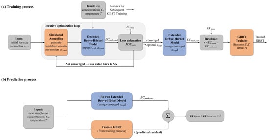
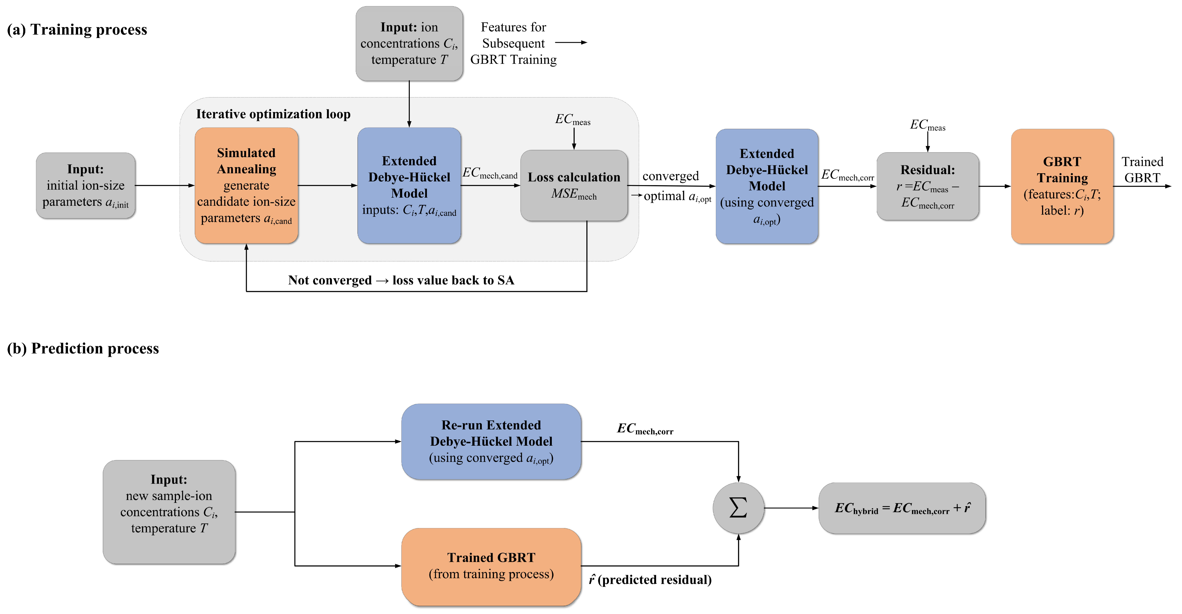
To improve the prediction accuracy of nutrient-solution electrical conductivity under complex multi-ion coupling conditions, this study proposes a novel two-stage hybrid modeling framework that integrates a classical electrolyte mechanistic model with a data-driven residual compensation strategy (Figure 1). The hybrid model consists of two sequentially executed modules: a calibrated extended Debye–Hückel (MDH) mechanistic module and a GBRT residual-correction module, termed CalMDH-ResGBRT in this work.

Figure 1. Schematic of the proposed CalMDH-ResGBRT two-stage physics–machine-learning hybrid model. The framework consists of two core workflows: (a) model training with physical parameter calibration and residual learning, and (b) EC inference for unknown nutrient-solution samples.

In the training stage (Figure 1a), the mechanistic model is first calibrated via parameter optimization to eliminate systematic baseline errors caused by empirical ionic-size parameters. After obtaining the optimized mechanistic predictions, the deviations between measured EC values and calibrated theoretical outputs are extracted as modeling residuals. Taking ion concentrations and solution temperature as input features and the residuals as training labels, the GBRT model is established to characterize the unmodeled higher-order ion interaction effects that cannot be quantified by conventional electrolyte theory.

In the inference stage (Figure 1b), the framework requires only ionic concentrations and ambient temperature as inputs. The calibrated mechanistic model provides physically consistent baseline EC values, while the pre-trained GBRT yields data-driven residual corrections. The final EC prediction is determined by superposing the baseline and residual terms. Notably, field-measured EC data participate only in model training and are completely independent of the prediction process, ensuring the generalization capability and physical interpretability of the proposed hybrid model.

2.2. Dataset Construction

To capture compositional variability under practical fertigation conditions, four base nutrient-solution formulations with distinct ionic ratios were designed to replicate typical nutrient regimes and ammonium–nitrate ratio adjustments for commercial soilless cultivation (Table 1). Each formulation contained seven major ions: K⁺, Ca²⁺, Mg²⁺, NH₄⁺, NO₃⁻, H₂PO₄⁻, and SO₄²⁻. One formulation was high in potassium and nitrate for fruit-vegetable production, another adopted an elevated ammonium-to-nitrate ratio to simulate nitrogen-supply conditions, and the remaining two adopted intermediate stoichiometries with varied Ca/Mg and P/S ratios. All solutions were prepared using analytical-grade reagents (Xilong Scientific Co., Ltd., Shantou, China): calcium nitrate tetrahydrate, potassium nitrate, ammonium dihydrogen phosphate, potassium dihydrogen phosphate, ammonium sulfate, magnesium sulfate heptahydrate, and magnesium nitrate hexahydrate.

Table 1. Formulations of the four basic nutrient solutions.

Base Mixture	Ion Concentration (mmol/L)							T (°C)	EC (μS/cm)
	K+	Ca2+	Mg2+	NH4+	NO3−	H2PO4−	SO42−
F1	8	4	2	1.3	16	1.3	2	25	2322
F2	7.5	2.25	0.75	4.5	12	3	1.5	25	1997
F3	7	2	3	3	12	4	2	25	1942
F4	3	1	0.5	1.5	5	1.5	0.5	25	847.9

Note: Values are the target ion concentrations of each base mixture, expressed in mmol/L; T, temperature (°C); EC, electrical conductivity (μS/cm). Based on the four base mixtures, a series of dilution gradients and temperature treatments was prepared to construct the dataset for EC prediction.

Serial dilution with deionized water was applied to each base formulation to generate concentration gradients covering an EC range of 6.6–2855 μS/cm, encompassing dilute seedling-stage solutions as well as full-strength growing-stage recipes. Corresponding single-salt solutions with identical dilution gradients were also prepared. Single-salt samples support ion-mobility calibration by constraining individual-ion transport behavior, while mixed-solution samples reproduce realistic multi-ion coupling effects. In total, 537 distinct solution compositions were generated.

All solutions were thermally equilibrated at one of five temperature levels (15–35 °C), covering typical seasonal greenhouse temperature fluctuations. Each dataset record consists of molar concentrations of the seven ions, solution temperature, and experimentally measured EC. Sample distribution across EC intervals, formulation types and temperature levels was inspected to ensure sufficient data coverage.

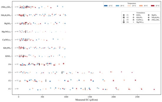
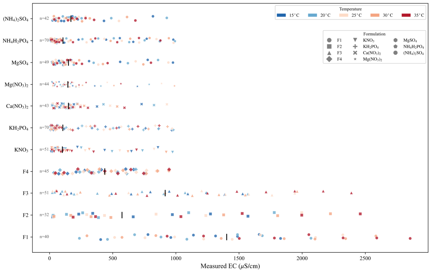
Electrical conductivity was measured with a multi-parameter water quality meter (HQ4300, Hach Company, Loveland, CO, USA) fitted with a CDC40103 four-pole graphite conductivity probe. The manufacturer-stated accuracy for conductivity is ±0.5% of reading, and the integrated temperature-sensor accuracy is ±0.3 °C. Built-in instrumental temperature compensation was disabled to record raw EC values at sample temperature instead of normalized values at 25 °C. Samples were stabilized in a thermostatic water bath, and thermal equilibrium was verified with a calibrated thermometer. Each solution was prepared once, and electrical conductivity was recorded as a single stable reading after signal stabilization. Neither replicate readings on the same solution nor independently prepared parallel samples were collected, so a type-A uncertainty evaluated from repeated observations cannot be obtained. Between measurements, the electrode was thoroughly rinsed using deionized water and dried to eliminate cross-contamination. The compiled nutrient-solution dataset is visualized in Figure 2, which illustrates the distribution of observations across different formulation types and temperature conditions.

Figure 2. Overview of the compiled nutrient-solution dataset. Each row represents one formulation type (F1–F4: mixed fertilizer formulations; the remaining rows: single-salt electrolyte solutions); data points are color-coded by temperature and shaped by formulation.

Stratified random sampling was used to partition the complete dataset into training and independent test sets at an 8:2 ratio. Stratification was performed over EC range, formulation type and temperature level to guarantee representative class proportions in both subsets.

Descriptive statistics including minimum, maximum, mean, median and standard deviation for the eight model-input features calculated from training-set samples are summarized in Table 2. Ion-concentration data exhibit strong right-skewed distributions, and several ion features show a median value of zero. This statistical characteristic originates from our experimental design, which includes single-salt solutions and heavily diluted samples alongside a small number of high-concentration stock-solution samples, rather than measurement errors or data defects.

Table 2. Descriptive statistics of input features in the training set.

Feature	Unit	Min	Max	Median	Mean	Std
K+	mmol/L	0	18.0	0.14	1.70	2.88
Ca2+	mmol/L	0	4.0	0	0.43	0.84
Mg2+	mmol/L	0	8.0	0	0.48	0.94
NH4+	mmol/L	0	18.0	0.06	1.07	2.43
NO3−	mmol/L	0	16.0	0.40	2.20	3.56
H2PO4−	mmol/L	0	18.0	0.20	1.51	3.17
SO42−	mmol/L	0	8.0	0	0.44	0.87
Temperature	°C	15.0	35.0	25.0	24.7	7.1

Although the ion-concentration distribution is heavily skewed, stratified random sampling was adopted for dataset partitioning. This strategy ensures that the training set fully covers the full range of ion concentrations and temperature relevant to practical fertigation, supporting reliable model training. Histogram-kernel density plots visualizing feature distributions are provided in Figure S1 (Supplementary Materials).

2.3. Mechanistic EC Model Based on the Extended Debye–Hückel Framework

The mechanistic model computes the electrical conductivity from the complete ionic composition by summing the contributions of all conducting species. For ion species with molar concentration c_i (mol/L) and charge number z_i, the solution ionic strength I is computed as:

$$I={\displaystyle \frac{1}{2}}{\sum }_{i=1}^n{c}_i{z}_i^2$$

(1)

where n denotes the total number of distinct ionic species in solution.

Over the ionic-strength range examined in this study, the finite size of hydrated ions substantially reduces ionic mobility. The single-ion activity coefficient ${\gamma }_i$ is computed from the extended Debye–Hückel equation:

$$\mathrm{l}\mathrm{o}\mathrm{g}{\gamma }_i=-{\displaystyle \frac{A{z}_i^2\sqrt{I}}{1+B{a}_i\sqrt{I}}}$$

(2)

where A and B are temperature-dependent solvent constants, and a_i denotes the ion-size parameter for ionic species $i$. At 25 °C, standard values are A = 0.509 (mol/L)^−1/2 and B = 3.281 (mol/L)^−1/2 nm⁻¹ [22]. For other temperatures, A and B are recalculated using water’s temperature-dependent dielectric constant ε(T) (a function of absolute temperature T, in Kelvin) from standard physical-chemistry references, $A=1.82 \times {10}^6{(\epsilon \left(T\right)\cdot T)}^{-3/2}$, $\mathrm{B}=50.3 \times (\epsilon \left(T\right)\cdot T{)}^{-1/2}$. The initial a_i, in units of ${10}^{-10} \mathrm{m}$, are 3.0 for ${\mathrm{K}}^{+}$, 6.0 for ${\mathrm{Ca}}^{2+}$, 8.0 for ${\mathrm{Mg}}^{2+}$, 2.5 for ${\mathrm{NH}}_4^{+}$, 3.0 for ${\mathrm{NO}}_3^{-}$, 4.5 for ${\mathrm{H}}_2{\mathrm{PO}}_4^{-}$, and 4.0 for ${\mathrm{SO}}_4^{2-}$ [18].

The limiting molar conductivities of the target ions at infinite dilution and 25 °C, denoted as ${\lambda }_{i,25}^{°}$, were taken from the literature: ${\mathrm{K}}^{+}$, ${\mathrm{Ca}}^{2+}$, ${\mathrm{Mg}}^{2+}$, ${\mathrm{NH}}_4^{+}$, ${\mathrm{NO}}_3^{-}$, ${\mathrm{H}}_2{\mathrm{PO}}_4^{-}$, and ${\mathrm{SO}}_4^{2-}$ are 73.5, 119.1, 106.1, 73.5, 71.4, 33.0, and 160.0 S cm²/mol, respectively [9,10]. These values were extrapolated to the measurement temperature through viscosity correction:

$${\lambda }_i^{°}\left(T\right)={\lambda }_{i,25}^{°}\cdot {\displaystyle \frac{{\eta }_{25}}{\eta \left(T\right)}}$$

(3)

where ${\lambda }_i^{°}\left(T\right)$ denotes the limiting molar ionic conductivity of the target ions at temperature T, η(T) denotes the dynamic viscosity of water at temperature T, and ${\eta }_{25}$ is the dynamic viscosity of water at 25 °C. This correction captures the dominant temperature dependence of ionic mobility over the 15–35 °C range [9,10,15]; the simplification ignores minor temperature drifts in ion-pair equilibria and hydration-shell structure.

The final mechanistically predicted EC (μS/cm) is obtained by summing the contributions of all ionic species:

$${EC}_{\mathrm{mech}} = {\sum }_{i=1}^n{c}_i{\gamma }_i{\lambda }_i^{°}(T)$$

(4)

2.4. Stage I: Simulated-Annealing Optimization of Ion-Size Parameters

The mechanistic model includes seven tunable ionic-size parameters. Literature nominal values derived from crystal or hydrated-radius measurements are not tailored for multi-component agricultural nutrient solutions. Since these parameters directly govern activity coefficients, they exert a pronounced effect on EC predictions, especially under high ionic-strength conditions. In Stage I, the mean squared error between mechanistic EC outputs and measured EC over the training dataset is minimized as the objective function:

$${\mathit{MSE}}_{\mathrm{mech}} = {\displaystyle \frac{1}{N}}{\displaystyle \sum _{j=1}^N}{({EC}_{\mathrm{m}\mathrm{e}\mathrm{c}\mathrm{h},j}-{EC}_{\mathrm{m}\mathrm{e}\mathrm{a}\mathrm{s},j})}^2$$

(5)

where N denotes the total number of training samples and j is the sample index.

The ionic-size parameters enter the model in a nonlinear fashion, and the objective function landscape exhibits multiple local minima, requiring a global optimization strategy. Simulated annealing (SA) was adopted owing to its gradient-free stochastic property and its ability to avoid local-optimum trapping. Compared with genetic algorithms and particle swarm optimization, SA involves fewer hyper-parameters and is well-suited for this seven-dimensional calibration task. For each parameter, the search space was defined as [0, 2 × a_i,nominal], corresponding to a ±100% interval relative to its literature nominal value.

Key SA hyper-parameters were configured as follows: maximum iterations of 20,000; a Markov-chain length of 400 at each temperature; and up to eight restarts. The initial temperature T₀ was determined empirically: 30 random parameter vectors were uniformly sampled, the standard deviation σ of the resulting training-set MSE was calculated, and T₀ = −σ/ln(0.2) was used to achieve an initial uphill-move acceptance probability of approximately 20%. Geometric cooling was applied with a cooling factor α = 0.001^(1/N) every 400 iterations, and the optimization terminates when the temperature decreases to 0.001 × T₀. An internal temperature-adjustment mechanism temporarily doubles the temperature if the chain acceptance rate drops below 5%, maintaining sufficient exploration capability.

At each Markov step, candidate parameter vectors are generated via Gaussian perturbation. One, two or three parameters are randomly selected with probabilities of 0.6, 0.3 and 0.1, respectively. Perturbations follow a normal distribution whose standard deviation equals 15% of the corresponding parameter’s search-range width and is further scaled by T/T₀ to gradually shrink step size during cooling. Perturbed parameters are clipped to stay within predefined bounds. Candidate solutions are accepted or rejected following the Metropolis criterion, where uphill transitions are accepted with probability $exp(-\Delta f/T)$. Multiple restarts were implemented to balance exploration and exploitation. The first restart was initialized using literature nominal values; subsequent restarts adopted two initialization strategies: 60% probability from the current global optimum superimposed with Gaussian noise and 40% probability by uniform random sampling over the full search domain.

After convergence, the optimized parameters are fed back into the mechanistic model to generate recalibrated baseline EC predictions over the training set. Several ionic-size parameters converged at the boundaries of the predefined search domain. These boundary-limited values are treated as apparent effective ionic-size parameters fitted for the present multi-ion nutrient-solution system, instead of intrinsic physical hydrated radii. The recalibrated mechanistic prediction is hereafter denoted ${\mathit{EC}}_{\mathrm{mech},\mathrm{corr}}$.

2.5. Stage II: Gradient-Boosting Regression Tree for Residual Compensation

Despite parameter calibration in Stage I, the calibrated extended Debye–Hückel (CalMDH) mechanistic model still produces systematic deviations from measured EC values. These residuals arise from higher-order multi-ion interactions, ion-pairing equilibria, and hydration-shell distortion, which cannot be fully captured by mean-field electrolyte theory. To account for these unmodelled nonlinear effects, this study employs a gradient-boosted regression tree (GBRT) to learn and correct the residuals between experimental observations and mechanistic baseline predictions.

2.5.1. Fundamental Properties of the GBRT Machine-Learning Component

The machine-learning module used for residual correction is built upon gradient-boosted regression tree principles. It constructs an additive ensemble of weak decision-tree learners. During training, the algorithm sequentially minimizes squared-error loss: each newly generated decision tree is fitted to the residuals of the preceding ensemble, and prediction results are aggregated across all base trees.

Notably, no mechanistic equations or physical constraints are embedded within the GBRT component itself. The GBRT does not directly predict absolute EC values for nutrient solutions. Instead, it is confined to predicting only residual deviations. All physical prior information and electrochemical constraints originate from the preceding standalone CalMDH mechanistic module, which supplies a physically consistent EC baseline, rather than being encoded inside the tree-model structure. The GBRT only compensates for those complex ionic phenomena that the electrolyte mechanistic theory cannot adequately describe.

2.5.2. Input–Output Configuration and Model Hyper-Parameters

For each training sample, the modeling residual is defined as:

$$r_j = {EC}_{\mathrm{m}\mathrm{e}\mathrm{a}\mathrm{s},j} -{ EC}_{\mathrm{m}\mathrm{e}\mathrm{c}h,\mathrm{c}\mathrm{o}\mathrm{r}\mathrm{r},j}$$

(6)

The input feature vector of the GBRT consists of eight variables: molar concentrations of the seven dominant ions and solution temperature. All input variables are standardized to zero mean and unit variance before model training to eliminate magnitude differences among features and accelerate convergence. The model takes residual $r_j$ as its training label and optimizes to minimize residual mean-squared error.

$${\mathit{MSE}}_{\mathrm{res}}={\displaystyle \frac{1}{N}}{\displaystyle \sum _{j=1}^N}{({\widehat{r}}_j-r_j)}^2$$

(7)

where ${\widehat{r}}_j$ is the GBRT-predicted residual for sample j.

Fixed hyper-parameters were adopted for the GBRT: 120 decision-tree base learners, maximum tree depth of 5, and a learning rate of 0.08. Stochastic subsampling with a fraction of 0.8 is applied in tree training: each tree is fitted on 80% of randomly selected samples without replacement, while all eight input features are available for node splitting.

2.5.3. Hybrid Inference Workflow

For unseen samples in the inference phase, the final EC output of the CalMDH-ResGBRT hybrid model is obtained by summing the calibrated mechanistic baseline and the residual correction predicted by the pre-trained GBRT:

$${\mathit{EC}}_{\mathrm{hybrid},j} = {EC}_{\mathrm{m}\mathrm{e}\mathrm{c}\mathrm{h},\mathrm{c}\mathrm{o}\mathrm{r}\mathrm{r},j}+{\widehat{r}}_j$$

(8)

Within this two-stage framework, the CalMDH module yields physically reasonable, monotonic EC responses against changes in ionic concentration and temperature within the data coverage range. The GBRT only compensates small-magnitude deviations originating from unmodelled multi-ion effects. Consequently, the hybrid framework retains the electrochemical interpretability afforded by the physical mechanistic description, while achieving substantial improvements in prediction accuracy via data-driven residual correction.

2.6. Benchmark Models and Evaluation Metrics

To quantitatively clarify the individual contributions of mechanistic parameter recalibration and data-driven residual compensation, three benchmark models were established for comparative analysis: (1) NomMDH, the conventional extended Debye–Hückel model utilizing literature-derived nominal ionic-size parameters; (2) CalMDH, the simulated-annealing calibrated mechanistic model with optimized ionic-size parameters but without residual correction; and (3) DirGBRT, a standalone GBRT model with identical input features and hyper-parameters as the residual-correction GBRT, which directly predicts full-scale EC values without mechanistic baseline inputs.

All models were trained and validated on identical training and test datasets following the same 8:2 stratified partitioning strategy. Five statistical metrics were adopted to comprehensively evaluate model performance on the independent test set, including the coefficient of determination R² for overall fitting capability, the root mean square error (RMSE) and mean absolute error (MAE) for absolute prediction accuracy, the mean absolute percentage error (MAPE) for relative error quantification, and the maximum absolute error (MaxAE) for characterizing extreme prediction deviation. To assess whether the observed performance differences depend on this specific single data partition, supplementary robustness tests were further carried out: five independent stratified 80/20 splits, together with stratified 5-fold and 10-fold cross-validation. All benchmark and hybrid models retained identical hyper-parameters in these supplementary evaluations, with only the data-splitting scheme varied.

3. Results

3.1. Correction of the Mechanistic Model Bias

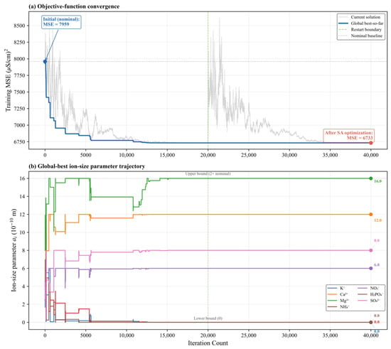
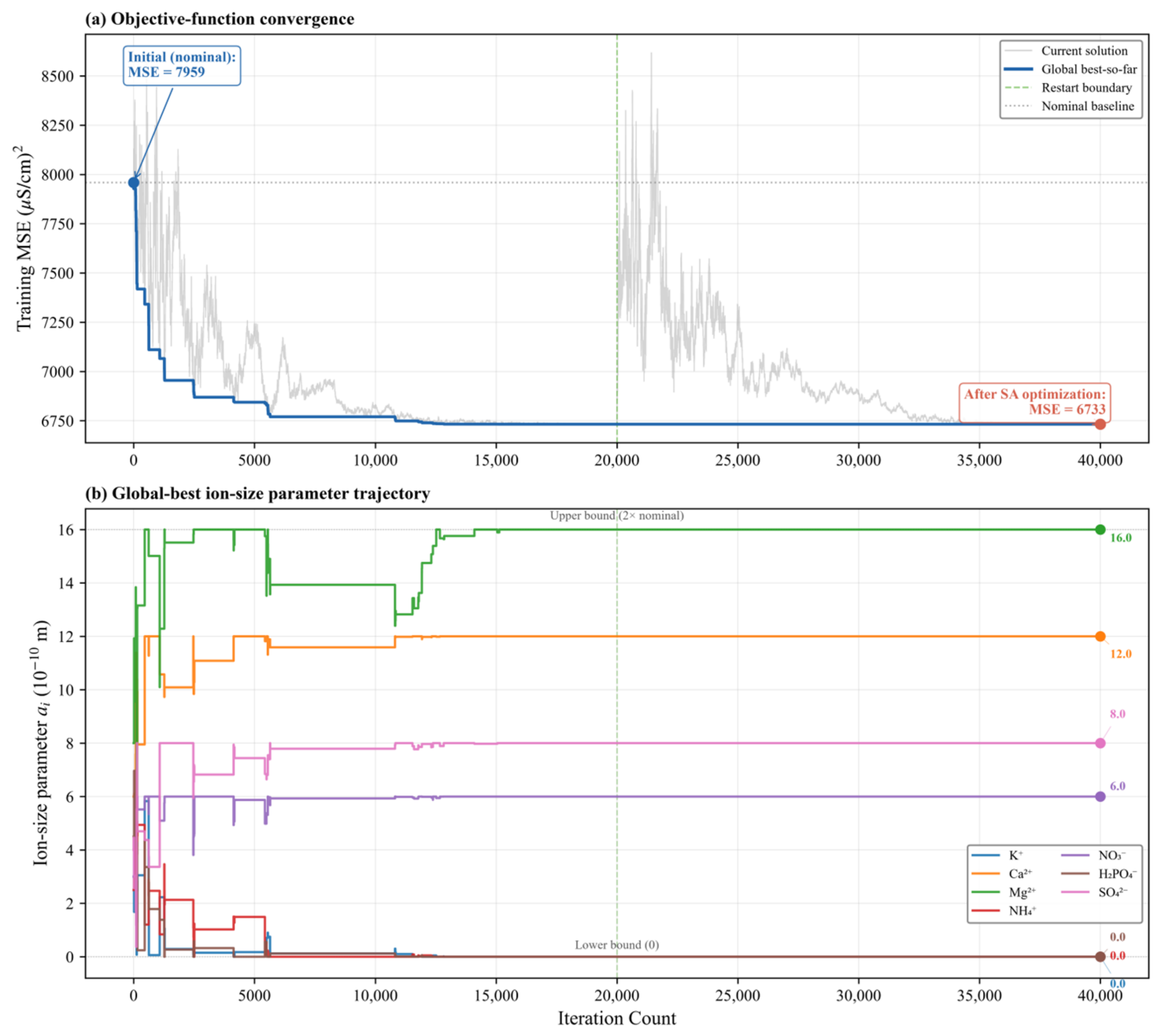
Stage-I simulated-annealing optimization yields moderate yet noteworthy improvements to the mechanistic model. Using literature nominal ionic-size parameters, the extended Debye–Hückel model achieves a training-set MSE of approximately 7959 (μS/cm)² (Figure 3).

Figure 3. Simulated-annealing convergence for ion-size parameter calibration of the extended Debye–Hückel model. Only two restart cycles are shown, as full convergence occurs within the first restart. (a) Convergence of the objective function; (b) evolution trajectories of the global-best ion-size parameters.

Following convergence achieved within the first of multiple configured restart cycles, the optimized parameters reduce the training-set MSE by 15.4%, decreasing from approximately 7959 to 6733 (μS/cm)², with RMSE dropping from 89.2 to 82.1 μS/cm (Figure 3a). Despite this limited overall improvement, a distinct boundary-convergence behavior is observed among optimized parameters: three monovalent ions (${\mathrm{K}}^{+}$, ${\mathrm{NH}}_4^{+}$, ${\mathrm{H}}_2{\mathrm{PO}}_4^{-}$) converge to the lower bound $a_i = 0$, which sets the Debye–Hückel denominator to unity and makes their activity coefficients nearly independent of ionic strength within the experimental range (Figure 3b). The remaining four ions (${\mathrm{Ca}}^{2+}$, ${\mathrm{Mg}}^{2+}$, ${\mathrm{NO}}_3^{-}$, ${\mathrm{SO}}_4^{2-}$) reach the upper limit of the predefined search domain. These boundary-limited values correspond to apparent effective parameters fitted for the present nutrient-solution system. Substantial structured residuals remain after parameter calibration, which are taken as the fitting target for the Stage-II model.

3.2. Performance of the Hybrid Model

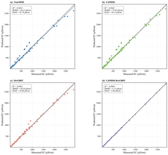
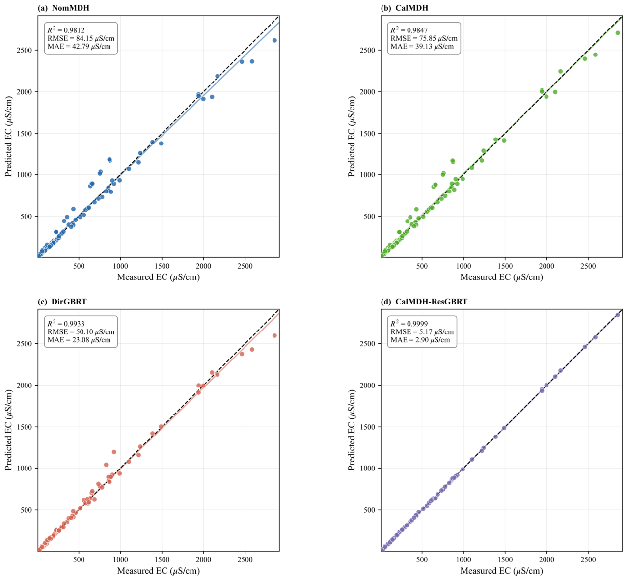
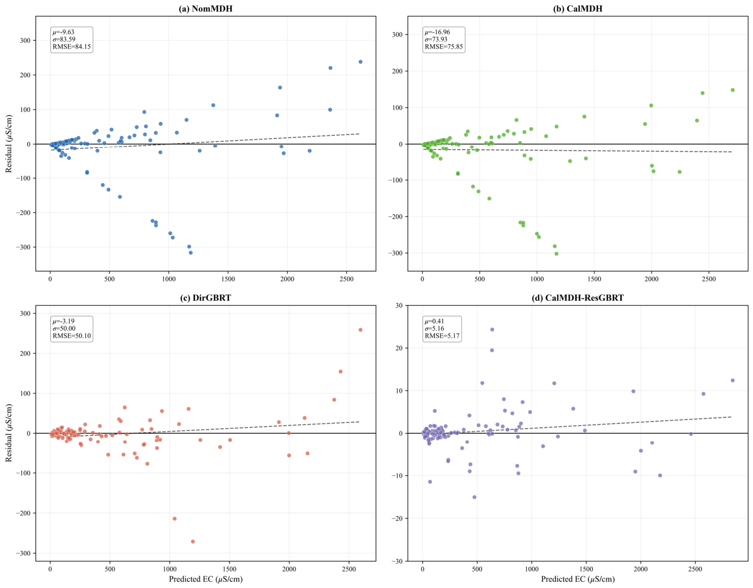
Based on the Stage-I calibrated mechanistic output, the Stage-II GBRT is trained on residuals between measured EC and CalMDH predictions. Evaluated on the independent test set containing 108 samples, the two-stage hybrid CalMDH-ResGBRT obtains an ${\mathrm{R}}^2 = 0.9999$ and an RMSE = 5.17 μS/cm (Figure 4d). The near-unity ${\mathrm{R}}^2$ indicates that the hybrid model accounts for nearly all variance in measured EC. The predicted values closely match experimental measurements over the full EC range, without obvious systematic bias at low or high concentration extremes.

Figure 4. Predicted versus measured EC on the held-out test set for (a) NomMDH, (b) CalMDH, (c) DirGBRT, and (d) CalMDH-ResGBRT. The dashed line denotes the 1:1 reference line, and the solid line is the regression line fitted to the scatter points. R², RMSE, and MAE are shown in each subplot.

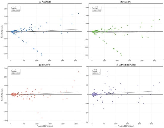
Residual analysis further demonstrates model performance. Figure 5 plots residuals derived from the difference between measured and predicted EC against predicted EC for all four models. Residuals of the hybrid model are evenly distributed around zero across the whole prediction range, with a standard deviation of 5.17 μS/cm and no obvious monotonic trend. Such random uniform scatter indicates the removal of structured systematic error components by the residual-learning module.

Figure 5. Residuals versus predicted EC for the four models on the held-out test set: (a) NomMDH, (b) CalMDH, (c) DirGBRT, and (d) CalMDH-ResGBRT. The solid horizontal line denotes the zero-residual line, and the dashed line represents the trend line fitted to the residuals. The mean residual (μ), residual standard deviation (σ), and RMSE are annotated in each subplot.

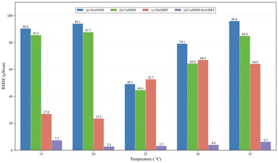
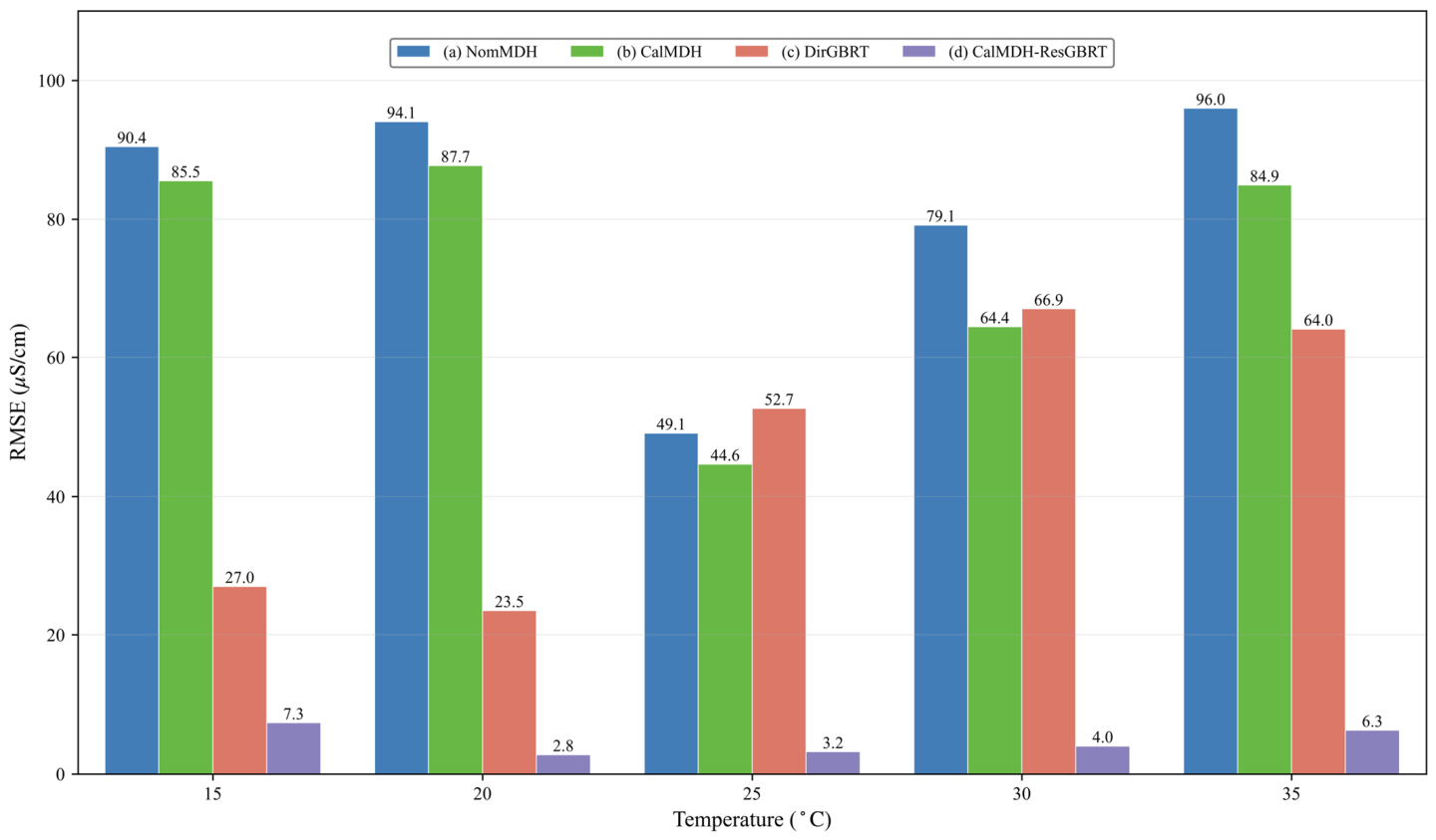
Figure 6 presents RMSE decomposed across five temperature levels (15, 20, 25, 30, and 35 °C). Across the full experimental temperature range covering both low-temperature and high-temperature endpoints as well as the intermediate central condition, CalMDH-ResGBRT achieves stable and remarkably low prediction errors. Its RMSE remains confined within a narrow band from 2.8 μS/cm to 7.3 μS/cm, with only minor error fluctuations observed over varying thermal conditions. Even at the extreme boundary temperatures of 15 °C and 35 °C, which constitute the limits of the investigated interpolation domain, the model does not suffer from error amplification.

Figure 6. Prediction RMSE of each model decomposed by temperature level (15, 20, 25, 30, and 35 °C).

3.3. Comparison with Benchmark Models

Quantitative predictive metrics for all four models are listed in Table 3, demonstrating progressive performance gains across model configurations. NomMDH yields an $R^2=0.9812$ and an RMSE = 84.15 μS/cm. CalMDH achieves an $R^2=0.9847$ and an RMSE = 75.85 μS/cm, representing an approximately 10% reduction in RMSE relative to NomMDH. The purely data-driven DirGBRT obtains an $R^2=0.9933$ and an RMSE = 50.10 μS/cm. The proposed hybrid CalMDH-ResGBRT returns an $R^2=0.9999$ and an RMSE = 5.17 μS/cm. Visual patterns of predicted-versus-measured EC are illustrated in Figure 4. Systematic over-prediction at mid-to-high EC values is observed for NomMDH in Figure 4. CalMDH retains visible systematic bias after parameter calibration. DirGBRT shows considerable scatter at high EC, whereas CalMDH-ResGBRT exhibits near-perfect agreement between predictions and measurements across the full EC range.

Table 3. Predictive performance of four models on the test set (n = 108).

Model	R2	RMSE (μS/cm)	MAE (μS/cm)	MAPE (%)	MaxAE (μS/cm)
NomMDH	0.9812	84.15	42.79	11.94	316.46
CalMDH	0.9847	75.85	39.13	11.41	302.06
DirGBRT	0.9933	50.10	23.08	7.03	270.84
CalMDH-ResGBRT	0.9999	5.17	2.90	1.32	24.32

Note: R², coefficient of determination; RMSE, root mean square error; MAE, mean absolute error; MAPE, mean absolute percentage error; MaxAE, maximum absolute error.

Distinct residual behaviors among models can be observed from Figure 5. NomMDH residuals exhibit obvious heteroscedasticity and increase with EC magnitude. CalMDH follows a similar residual pattern with reduced amplitude. DirGBRT produces more random residuals but still contains local bias. Only the hybrid model yields residuals uniformly scattered around zero throughout the modeling domain, free of structured deviations.

As revealed by Figure 6 across five temperature levels, the three benchmark models universally suffer performance degradation at low- and high-temperature boundaries of the interpolation domain. NomMDH and CalMDH maintain large RMSE values over the whole temperature range, while the purely data-driven DirGBRT presents sharply elevated errors near temperature boundaries, reflecting its unsatisfactory robustness at the boundaries of the interpolation domain. By contrast, the hybrid model avoids such temperature-induced performance decay.

Compared with the three benchmark approaches, the hybrid model achieves 89.7–93.9% reduction in test-set RMSE. Corresponding MAE reductions reach 93.2%, 92.6% and 87.4% relative to NomMDH, CalMDH and DirGBRT, respectively. Noticeable improvement is also observed for maximum absolute error: the worst-case error of the hybrid model is 24.32 μS/cm, which is roughly 1/12–1/13 of MaxAE values from benchmark models. These quantitative results demonstrate that the combination of mechanistic recalibration and data-driven residual correction outperforms either component alone, and it mitigates the boundary-related performance loss that widely exists in baseline models under varying-temperature operating conditions.

3.4. Robustness Under Multiple Random Data Partitions

To examine whether the large performance gap among models arises from a fortunate single 8:2 partition, supplementary robustness evaluations were conducted for all four models with fixed hyper-parameters, including five independent stratified 80/20 splits and stratified 5-fold and 10-fold cross-validation.

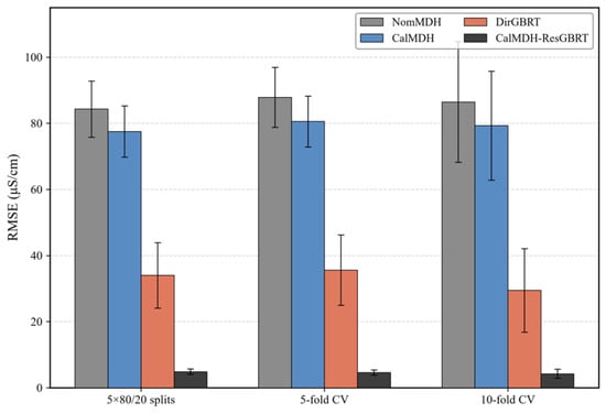
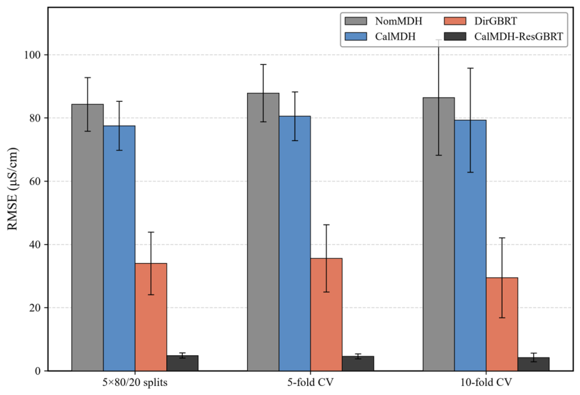
Figure 7 summarizes RMSE values across different splitting strategies. CalMDH-ResGBRT consistently maintains low RMSE values ranging from 4.25 to 4.87 μS/cm under all three partitioning schemes, far below the values of the three baseline models. All models show some RMSE fluctuations (error bars), yet the model performance ranking remains unchanged. Despite high near-unity R² values for all models, this metric conceals large absolute prediction errors for baseline models, so RMSE is more informative for practical EC prediction.

Figure 7. RMSE of four models under different data-splitting robustness tests. Error bars denote standard deviation calculated across repeated runs. All model hyper-parameters remained fixed during evaluation.

These observations demonstrate that the prominent accuracy advantage of CalMDH-ResGBRT is not a statistical artifact originating from one favorable train–test partition. Full numerical results including R², RMSE, MAE, MAPE and MaxAE for every model under each splitting scheme are provided as a downloadable Supplementary Data File.

4. Discussion

4.1. Interpretation of Simulated-Annealing-Driven Recalibration of Ionic-Size Parameters

The simulated-annealing optimization of ion-size parameters delivered only a moderate global reduction in training-set error, even though the optimization yielded boundary-limited fitted parameters with meaningful physical implications for multi-component soilless-cultivation nutrient solutions. After SA calibration, the training-set RMSE only decreased from 89.2 to 82.1 μS/cm, which indicates that adjusting single-ion-size parameters within the extended Debye–Hückel framework cannot fully eliminate systematic deviations for agricultural fertigation solutions. It should be emphasized that these boundary-hit parameters should be interpreted as system-specific apparent effective parameters rather than intrinsic hydrated ionic radii obtained from simple single-salt electrolyte measurements. Such boundary convergence emerges from the aggregated effects of ion-pair association, competitive hydration, and many-body electrostatic interactions under multi-ion fertigation conditions.

As a mean-field electrolyte approximation, the extended Debye–Hückel theory describes inter-ionic interactions via averaged electrostatic potentials and treats ion hydration only through a single size parameter for each ionic species. Consequently, it cannot directly capture cation-anion pairing or concentration-dependent distortion of hydration shells, both of which reduce the concentration of charge-carrying free ions and generate structured residuals [17,18]. Parameter optimization can only partially align the mechanistic baseline to average experimental observations. Therefore, the SA-calibrated mechanistic module serves as a physically grounded baseline, while the remaining structured nonlinear deviations are delegated to GBRT residual compensation in Stage II.

This challenge is not unique to nutrient solutions. Multi-component activity-coefficient formulations [16] and semi-empirically calibrated conductivity models [19,21] have been developed to address the degradation of accuracy in mean-field limiting laws with rising solute concentration. Systematic comparisons of calculation schemes further reveal that the achievable prediction accuracy is governed by the treatment of ionic speciation and parameterization [13]. Within the concentration range relevant to practical production, activity-based estimators for nutrient solutions can reproduce measured EC with coefficients of determination exceeding 0.99 [22]. Nevertheless, the resulting residuals are structured instead of random. Stage II is constructed to learn this structured residual component, rather than the global trend already captured by the mechanistic backbone.

4.2. Super-Additive Synergy of the Two-Stage CalMDH-ResGBRT Hybrid Architecture

The remarkable prediction accuracy of the proposed hybrid model arises from task-specialized decomposition into a physical mechanistic component and a machine-learning correction component, yielding clear super-additive performance beyond either component alone. When operated independently, CalMDH produces large systematic bias at moderate-to-high ionic strength, while the end-to-end purely data-driven DirGBRT achieves decent interpolation accuracy but suffers unstable performance across temperature gradients even within the interpolation domain. By contrast, the CalMDH-ResGBRT framework entrusts the calibrated Debye–Hückel backbone with capturing dominant and smooth physical variations in electrical conductivity that vary with ionic strength and temperature. This framework constrains the GBRT module to exclusively fit low-magnitude residuals derived from higher-order ionic phenomena that cannot be explicitly described by conventional physical models.

This separation of responsibilities brings two critical advantages. First, the GBRT module does not expend model capacity to rediscover well-established electrolyte physics; instead, its full representational power is focused on hard-to-model nonlinear effects including ion pairing and hydration-shell perturbation. Second, temperature-dependent ionic mobility governed by solvent viscosity is intrinsically encoded within the mechanistic component. As evidenced in Figure 6, DirGBRT showed obvious RMSE elevation near temperature boundaries of the measured range because purely data-driven learning lacks embedded electrochemical constraints and generalizes poorly for temperature conditions sparsely sampled within training data. Benefiting from the physics-based temperature correction, CalMDH-ResGBRT maintained consistently low prediction error across 15–35 °C, demonstrating enhanced robustness under variable greenhouse thermal environments.

For context, data-driven predictors reported for comparable soilless systems perform considerably worse in absolute terms. A CatBoost model for lettuce nutrient solutions obtained an R² = 0.946 with an EC RMSE of 248.28 µS/cm [30], and soft-sensor models inferring individual fertilizer-component concentrations in mixed variable-rate fertigation reported R² values of 0.989–0.997 [25]. Because nutrient-solution datasets generally span a wide EC range (6.6–2855 µS/cm in this study), coefficients of determination close to unity can coexist with absolute errors that still compromise fertigation dosing decisions. This artifact originates from high total variance within the measured EC dataset, where the standard deviation reaches 539 μS/cm. Even models with non-negligible absolute prediction errors can still yield near-unity R² values. For instance, the standalone DirGBRT achieved an R² > 0.993 but retained an RMSE of approximately 30–50 μS/cm across repeated data partitions. A high R² merely quantifies the proportion of total dataset variance explained by the model and cannot reflect the magnitude of absolute prediction error, which constitutes the key practical metric for fertigation control. Therefore, RMSE and MAE should be prioritized for performance assessment of nutrient-solution EC prediction.

Error decomposition further reveals the source of performance improvement for the hybrid framework. Simulated-annealing-driven calibration of ion-size parameters only delivers moderate error reduction, decreasing RMSE roughly by 8% from NomMDH to CalMDH. The dominant accuracy gain originates from the residual-learning GBRT component, which compensates structured deviations caused by higher-order ionic interactions, ion pairing and hydration-shell distortion that cannot be captured by the mean-field extended Debye–Hückel theory. By shifting the burden of learning major smooth physical variations to the calibrated mechanistic module, the GBRT only fits low-magnitude residuals, substantially lowering the learning difficulty for the tree-based learner and yielding much smaller prediction errors.

The architecture belongs to the residual-correction family of physics-informed machine learning, in which a mechanistic model supplies a physically constrained baseline and a learner fits only the deviations, rather than the governing equations being embedded in the loss function of the learner [33]. Reviews of hybrid and physics-informed models in soil–water and agricultural systems report gains in parameterization, transferability and interpretability relative to either component alone [32]; comparable residual-correction designs have improved evapotranspiration estimates over croplands without ground-based recalibration [34], and the coupling of process-based with data-driven models is regarded as a promising architecture for water-quality monitoring and prediction [35].

4.3. Practical Implications for Precision Soilless-Cultivation Fertigation

Electrical conductivity acts as the primary process indicator for water–fertilizer integration systems [5,6]. Purely data-driven models risk generating physically implausible outputs for novel nutrient formulations inadequately represented in training data, which may mislead fertilizer dosage adjustment [32,33]. The hybrid framework mitigates this risk: final EC prediction is dominated by the physically consistent CalMDH baseline, while residual corrections contributed by GBRT remain comparatively small. Even for inputs deviating from the training distribution, predicted EC retains physically reasonable monotonic correlations with ion concentration and temperature, supporting graceful performance degradation rather than catastrophic failure.

In practical application scenarios, the high-accuracy hybrid model enables offline pre-screening of candidate nutrient recipes before laboratory mixing and measurement, substantially reducing experimental workload for formulation development [3]. Moreover, it facilitates feedforward fertigation control: given target ion concentrations, EC can be pre-computed to pre-adjust fertilizer pump outputs before sensor feedback becomes available, complementing conventional sensor-based closed-loop regulation [5,37,38]. Achieving prediction RMSE below 10 μS/cm meets the accuracy requirement for practical precision fertigation under the composition and temperature ranges covered in this study.

Realization of feedforward control requires prior knowledge of the ionic composition supplied to the prediction model. Ion-specific sensing technologies are undergoing rapid development: a portable multiplexed ion-selective electrode array with MOF-based solid contacts has been validated for long-term monitoring, capacitively coupled contactless conductivity detection supports rapid multi-ion quantification, and online automatic water-fertilizer blending systems are under development for raw water formulation [39,40]. Integrating the proposed prediction model with such sensing hardware can realize a closed workflow spanning ionic composition measurement to fertilizer dosing actuation.

4.4. Limitations and Outlook

This work has several identifiable constraints. The dataset is built around seven major ions common in hydroponic fertigation; specialty ions such as chloride, chelated-iron species and borate are not included, so further experimental calibration will be required to extend model applicability to these ionic components.

Potential leakage caused by serially diluted samples is an intrinsic dataset property and equally impacts all models under identical partitioning. Even within one dilution series with fixed ion ratios, ion-activity and ion-pair effects produce nonlinear conductivity–concentration relationships, so diluted samples are not trivial duplicates of one another, which mitigates performance inflation driven by sample similarity. Repeated experiments under multi-seed 80/20 splits together with 5-fold and 10-fold cross-validation show that baseline models consistently yield worse accuracy under identical partitions, implying that the advantage of CalMDH-ResGBRT originates mainly from its physics-guided hybrid structure rather than splitting leakage. Nevertheless, sample-wise random division cannot fully exclude this bias. Rigorous Leave-One-Formulation-Out cross-validation and unseen-temperature holdout tests were not performed due to the limited number of base stock solutions and should be addressed in future studies with richer datasets.

From the mechanistic perspective of the model, the mechanistic backbone does not explicitly incorporate mass-action equations for ion-pair equilibria; explicitly introducing ion-pair formation constants may further reduce residual magnitude, albeit introducing additional parameters requiring fitting. It should be noted that the viscosity-ratio temperature correction in Equation (3) is derived from the empirical Walden’s rule. This simplified approximation captures the dominant temperature effect induced by solvent viscosity, while temperature-dependent changes in water dielectric constant and ionic-association equilibrium are not explicitly considered. From the model residuals shown in Figure 6, we infer that the temperature-dependent error learned by the GBRT component partially compensates for these omitted physical effects, which represents an inherent characteristic and limitation of this hybrid modeling framework. Although the hybrid model shows improved physical plausibility at the boundaries of the training interpolation domain, dedicated out-of-distribution extrapolation validation is still absent.

Future work may focus on: (i) expanding experimental datasets covering additional ionic species and performing systematic extrapolation tests; (ii) embedding explicit ion-pairing equilibrium into the mechanistic module to reduce reliance on machine-learning residual correction; and (iii) developing novel nutrient-solution dispensing systems based on the proposed model.

5. Conclusions

This study proposed a two-stage hybrid modeling framework that integrates the extended Debye–Hückel electrolyte mechanistic model with gradient-boosted regression tree residual compensation for electrical conductivity prediction of multi-ion mixed fertilizer nutrient solutions for soilless cultivation. By applying simulated annealing to optimize the ion-size parameters of the mechanistic model, the systematic baseline bias originating from dilute-solution assumptions was partially alleviated, and the subsequent GBRT module further fitted and corrected the structured residuals caused by unmodeled higher-order ionic interactions, ion pairing and hydration-shell distortion. Validated on a dataset containing 537 samples covering four mixed nutrient formulations, seven single-salt electrolytes, EC ranging from 6.6 to 2855 μS/cm and temperatures from 15 °C to 35 °C, the hybrid model achieved an R² = 0.9999 and an RMSE = 5.17 μS/cm on the independent test set, yielding 89.7–93.9% error reduction compared with the nominal mechanistic model, calibrated mechanistic model and purely data-driven GBRT baseline. Benefiting from the physical constraints embedded in the mechanistic backbone, the proposed approach maintained stable high-precision prediction across the whole experimental temperature range and avoided the performance deterioration at temperature boundaries observed in benchmark models. Compared with pure mechanistic models and end-to-end machine-learning models, this hybrid method realizes the combination of electrochemical interpretability, high interpolation accuracy and improved physical plausibility of outputs. It can support offline pre-screening of nutrient solution recipes and feedforward control of integrated water–fertilizer systems, providing an effective prediction tool for precision fertigation in soilless cultivation.

References

- Sambo, P.; Nicoletto, C.; Giro, A.; Pii, Y.; Valentinuzzi, F.; Mimmo, T.; Lugli, P.; Orzes, G.; Mazzetto, F.; Astolfi, S.; et al. Hydroponic solutions for soilless production systems: Issues and opportunities in a smart agriculture perspective. Front. Plant Sci. 2019, 10, 923. [Google Scholar] [CrossRef] [Scilit]
- Wu, J.Y.; Li, T.Y.; Li, J.J.; Chen, D.; Zhang, Q.W. Horticultural strategies for enhancing yield and quality in hydroponic microgreens: A comprehensive review. Horticulturae 2026, 12, 595. [Google Scholar] [CrossRef] [Scilit]
- Moreira Barradas, J.M.; Dida, B.; Matula, S.; Dolezal, F. A model to formulate nutritive solutions for fertigation with customized electrical conductivity and nutrient ratios. Irrig. Sci. 2018, 36, 133–142. [Google Scholar] [CrossRef] [Scilit]
- Hong, Y.; Lee, J.; Park, S.; Kim, J.; Jang, K.-J. Next-generation nitrate, ammonium, phosphate, and potassium ion monitoring system in closed hydroponics: Review on state-of-the-art sensors and their applications. AgriEngineering 2024, 6, 4786–4811. [Google Scholar] [CrossRef] [Scilit]
- Sulaiman, H.; Yusof, A.A.; Mohamed Nor, M.K. Automated hydroponic nutrient dosing system: A scoping review of pH and electrical conductivity dosing frameworks. AgriEngineering 2025, 7, 43. [Google Scholar] [CrossRef] [Scilit]
- Naseem, M.T.; Zaman, W. Root-zone engineering in closed soilless horticulture: From plant physiology to sensor-guided control. Horticulturae 2026, 12, 1088. [Google Scholar] [CrossRef] [Scilit]
- Bannon, S.P.; Thomas, J.; Webster, R.J.; Whitby, H. Temporal variation of nutrient ratios within hydroponic nutrient solutions. Food Energy Secur. 2026, 15, e70220. [Google Scholar] [CrossRef] [Scilit]
- Wu, M.L.; Niu, W.Q.; Wen, S.L.; He, Z.L.; Li, X.K. Electrical conductivity method for measuring concentrations of diammonium hydrogen phosphate and potassium chloride in their mixed solution. J. Irrig. Drain. 2021, 40, 71–78. (In Chinese) [Google Scholar]
- Shcherbakov, V.V.; Artemkina, Y.M. Limiting equivalent electrical conductivity of inorganic salt solutions and dielectric properties of a polar solvent. Russ. J. Inorg. Chem. 2013, 58, 968–971. [Google Scholar] [CrossRef] [Scilit]
- McCleskey, R.B. Electrical conductivity of electrolytes found in natural waters from (5 to 90) °C. J. Chem. Eng. Data 2011, 56, 317–327. [Google Scholar] [CrossRef] [Scilit]
- McCleskey, R.B.; Nordstrom, D.K.; Ryan, J.N. Electrical conductivity method for natural waters. Appl. Geochem. 2011, 26, S227–S229. [Google Scholar] [CrossRef] [Scilit]
- McCleskey, R.B.; Nordstrom, D.K.; Ryan, J.N.; Ball, J.W. A new method of calculating electrical conductivity with applications to natural waters. Geochim. Cosmochim. Acta 2012, 77, 369–382. [Google Scholar] [CrossRef] [Scilit]
- McCleskey, R.B.; Nordstrom, D.K.; Ryan, J.N. Comparison of electrical conductivity calculation methods for natural waters. Limnol. Oceanogr. Methods 2012, 10, 952–967. [Google Scholar] [CrossRef] [Scilit]
- Endoh, S.; Tsujii, I.; Kawashima, M.; Okumura, Y. A new method for temperature compensation of electrical conductivity using temperature-fold dependency of fresh water. Limnology 2008, 9, 159–161. [Google Scholar] [CrossRef] [Scilit]
- McCleskey, R.B. New method for electrical conductivity temperature compensation. Environ. Sci. Technol. 2013, 47, 9874–9881. [Google Scholar] [CrossRef] [Scilit]
- Zaveri, R.A.; Easter, R.C.; Wexler, A.S. A new method for multicomponent activity coefficients of electrolytes in aqueous atmospheric aerosols. J. Geophys. Res. Atmos. 2005, 110, D02201. [Google Scholar] [CrossRef] [Scilit]
- Senik, Y.; Pismenskaya, N.; Nikonenko, V.; Pourcelly, G. A model for calculating ion equilibria and electrical conductivity of natural water solutions. Desalination 2006, 191, 232–235. [Google Scholar] [CrossRef] [Scilit]
- Li, M.Y.; Fang, T. Modeling for mean ion activity coefficient of strong electrolyte system with new boundary conditions and ion-size parameters. Chin. J. Chem. Eng. 2015, 23, 1169–1177. [Google Scholar] [CrossRef] [Scilit]
- Zhang, W.T.; Chen, X.; Wang, Y.; Wu, L.Y.; Hu, Y.D. Experimental and modeling of conductivity for electrolyte solution systems. ACS Omega 2020, 5, 22465–22474. [Google Scholar] [CrossRef] [Scilit]
- Visconti Reluy, F.; de Paz Bécares, J.M.; Zapata Hernández, R.D.; Sánchez Díaz, J. Development of an equation to relate electrical conductivity to soil and water salinity in a Mediterranean agricultural environment. Aust. J. Soil Res. 2004, 42, 381–388. [Google Scholar] [CrossRef] [Scilit]
- Visconti, F.; De Paz, J.M.; Rubio, J.L. An empirical equation to calculate soil solution electrical conductivity at 25 °C from major ion concentrations. Eur. J. Soil Sci. 2010, 61, 980–993. [Google Scholar] [CrossRef] [Scilit]
- Song, J.X.; Xu, L.; He, D.X.; Tuskagoshi, S.; Kozai, T.; Shinohara, Y. Estimating EC and ionic EC contribution percentage of nutrient solution based on ionic activity. Int. J. Agric. Biol. Eng. 2019, 12, 42–48. [Google Scholar] [CrossRef] [Scilit]
- Abioye, E.A.; Hensel, O.; Esau, T.J.; Elijah, O.; Abidin, M.S.Z.; Ayobami, A.S.; Yerima, O.; Nasirahmadi, A. Precision irrigation management using machine learning and digital farming solutions. AgriEngineering 2022, 4, 70–103. [Google Scholar] [CrossRef] [Scilit]
- Kim, M.Y.; Park, G.; Seo, C.H. Application of artificial intelligence and machine learning in vertical farming: A comprehensive review. Sustainability 2026, 18, 8261. [Google Scholar] [CrossRef] [Scilit]
- Wu, M.L.; Xiong, J.J.; Li, R.Y.; Dong, A.H.; Lv, C.; Sun, D.; Abdelghany, A.E.; Zhang, Q.; Wang, Y.Q.; Siddique, K.H.M.; et al. Precision forecasting of fertilizer components’ concentrations in mixed variable-rate fertigation through machine learning. Agric. Water Manag. 2024, 298, 108859. [Google Scholar] [CrossRef] [Scilit]
- Sodini, M.; Cacini, S.; Navarro, A.; Traversari, S.; Massa, D. Estimation of pore-water electrical conductivity in soilless tomatoes cultivation using an interpretable machine learning model. Comput. Electron. Agric. 2024, 218, 108746. [Google Scholar] [CrossRef] [Scilit]
- Ma, Y.; Wu, Z.; Cheng, Y.; Chen, S.; Li, J. Rapid detection of fertilizer information based on near-infrared spectroscopy and machine learning and the design of a detection device. Agriculture 2024, 14, 1184. [Google Scholar] [CrossRef] [Scilit]
- Tuan, V.N.; Dinh, T.D.; Zhang, W.; Khattak, A.M.; Le, A.T.; Saeed, I.A.; Gao, W.; Wang, M. A smart diagnostic tool based on deep kernel learning for on-site determination of phosphate, calcium, and magnesium concentration in a hydroponic system. RSC Adv. 2021, 11, 11177–11191. [Google Scholar] [CrossRef] [Scilit]
- Tuan, V.N.; Khattak, A.M.; Zhu, H.; Gao, W.L.; Wang, M.J. Combination of multivariate standard addition technique and deep kernel learning model for determining multi-ion in hydroponic nutrient solution. Sensors 2020, 20, 5314. [Google Scholar] [CrossRef] [Scilit]
- Wei, C.; Li, Z.; Zhu, D.; Xu, T.; Liang, Z.; Liu, Y.; Zhao, N. Regulation of the physicochemical properties of nutrient solution in hydroponic system based on the CatBoost model. Comput. Electron. Agric. 2025, 229, 109729. [Google Scholar] [CrossRef] [Scilit]
- Sun, Z.T.; Yan, H.R.; Yang, Y.X.; Sun, D.H.; Hu, X.D.; Hu, J. Control system of nutrient solution for hydroponic lettuce based on ion activity. Trans. Chin. Soc. Agric. Mach. 2025, 56, 288–299. [Google Scholar]
- Filipowicz, P.; Saletnik, B. Hybrid and physics-informed AI models for soil water dynamics in sustainable agriculture—A review. Sustainability 2026, 18, 7452. [Google Scholar] [CrossRef] [Scilit]
- Karniadakis, G.E.; Kevrekidis, I.G.; Lu, L.; Perdikaris, P.; Wang, S.; Yang, L. Physics-informed machine learning. Nat. Rev. Phys. 2021, 3, 422–440. [Google Scholar] [CrossRef] [Scilit]
- Dobrokhotov, A.; Lopez, O.; Kozyreva, L.; Mukhina, D. A machine learning residual correction framework for enhancing physical-based evapotranspiration estimates over croplands. Eur. J. Remote Sens. 2026, 59, 2695909. [Google Scholar] [CrossRef] [Scilit]
- Wang, P.; Zou, S.; Li, J.; Ju, H.; Zhang, J. Advancing water quality management: Harnessing the synergy of remote sensing, process-based models, and machine learning to enhance monitoring and prediction. Remote Sens. 2025, 17, 3157. [Google Scholar] [CrossRef] [Scilit]
- Guo, J.; Chai, Y.; Hong, C.; Liu, H.; Xie, L.; Wang, T.; Chen, J.; Song, G.; Yi, Z.; Su, F. Prediction of the low-temperature properties of electrolyte solvents for lithium-ion batteries via machine learning. Nanoscale 2026, 18, 2613. [Google Scholar] [CrossRef] [Scilit]
- Li, J.N.; Wu, J.; Zhang, J.; Su, Z.Y.; Chen, X.H.; Fang, J.L. Development of an online automatic water–fertilizer mixing device considering direct mixing of raw water. Agriculture 2026, 16, 3. [Google Scholar] [CrossRef] [Scilit]
- Jin, Z.; Zhang, J.; Guo, H.; Hu, Y.; Chen, X.; Huang, H.; Wang, H. Development and testing of intelligent sensing and precision proportioning system of water and fertilizer concentration. Smart Agric. 2020, 2, 2. (In Chinese) [Google Scholar]
- Abdollahzadeh, M.; Zhu, Y.J.; Bayatsarmadi, B.; Vepsäläinen, M.; Razmjou, A.; Murugappan, K.; Rodopoulos, T.; Asadnia, M. Portable multiplexed ion-selective sensor for long-term and continuous irrigation water quality monitoring. Comput. Electron. Agric. 2024, 227, 109455. [Google Scholar] [CrossRef] [Scilit]
- Zhang, J.Q.; Chen, X.Y.; Wang, R.J.; Liu, Y.; Li, W.; Li, M.Y. Development and experiment of the rapid detection device of the nutrient ion concentrations for fertigation system. Trans. Chin. Soc. Agric. Eng. 2022, 38, 102–110. (In Chinese) [Google Scholar]
Disclaimer/Publisher’s Note: The statements, opinions and data contained in all publications are solely those of the individual author(s) and contributor(s) and not of MDPI and/or the editor(s). MDPI and/or the editor(s) disclaim responsibility for any injury to people or property resulting from any ideas, methods, instructions or products referred to in the content. |
© 2026 by the authors. Licensee MDPI, Basel, Switzerland. This article is an open access article distributed under the terms and conditions of the Creative Commons Attribution (CC BY) license.