A Thermal Time-Constant Framework for Temperature Forecasting and Control in Commercial Broiler Houses

Abstract

Accurate indoor-temperature forecasting underpins feed-forward control in broiler production, yet the horizons at which data-driven models add value are unclear. Two questions are addressed: at which horizons learned models measurably beat persistence, and what preview a feed-forward controller needs. Thirty-five days of data at 15 min resolution from a commercial stacked-cage broiler house (78,000 birds; outdoor temperature $-19$ to 16 °C) are used to benchmark 18 single-step and 10 multi-horizon models, probabilistic forecasts, and control simulation. A single time constant, $\tau =25.7$ h, organises the results: at 15 min, all learned models collapse to the persistence baseline (RMSE ≈ 0.105 K), because only 1% of the response relaxes per step; significant gains appear only at ≈$1\tau$ (LSTM $-25$% at 24 h, $-30$% at 48 h; FDR q ≤ 0.031). In control simulation, 4–8 h of MPC preview held $\sigma$ = 0.17 K with zero violations (0.74 K for 1 h control), while longer horizons added no benefit and were less robust. Quantile intervals calibrated in-sample (PICP ≈ 0.90) under-covered under distribution shift (0.61–0.72); $\tau$-anchored bands stayed calibrated (0.92–0.97). Design rules: evaluate forecasting models at horizons of at least ≈$1\tau$ and set control preview to ≈0.7–1.5${\tau }_f$, re-estimated per house and season.

1. Introduction

In winter, commercial broiler houses operate under tight set-point control: ventilation dampers and heaters balance the metabolic heat of tens of thousands of birds against outdoor conditions that fall below $-19$ °C [1,2]. Indoor temperature is the primary environmental variable in broiler production, directly affecting growth rate and feed conversion [3,4]; deviations in either direction are costly, and the heat-stress side of this problem has received the larger share of research attention [5,6]. The winter control problem is difficult not because the physics is unknown, but because the system is slow: the building fabric, birds, and floor store heat on time scales that far exceed the 15 min control interval of typical climate controllers.

A large body of research applies statistical and machine learning models to predict livestock-house temperature, including physics-based heat-balance models [7,8,9], dynamic thermal-load simulations [10], and models that explicitly account for building thermal mass [11], as well as steady-state balance approaches [8,9], linear time-series models [12,13], and tree ensembles [14,15]. Among deep networks, recurrent architectures [16], attention mechanisms [17], temporal convolutions [18], and basis-expansion models [19] have all been applied to time-series forecasting. Reported accuracies are high (RMSE ≈ 0.1–0.5 K at 10–30 min horizons) [12]. However, nearly all studies compare models at a single horizon without explaining why the achievable accuracy is what it is or indicating when a more complex model actually pays off. Two practical questions therefore remain open. First, at what prediction horizon do data-driven models provide statistically significant gains over trivial baselines [20,21]? Second, what prediction horizon should a feed-forward temperature controller use [22]? Neither question can be answered by a model comparison alone; both require a physical measure of how fast the controlled system actually responds.

A complementary body of work characterises the indoor thermal environment from the airflow side, describing where temperature varies within a house rather than how fast it changes. Computational fluid dynamics (CFD) studies have mapped airflow and temperature distributions in broiler and layer houses [23,24,25], including recent microclimate simulations of fully stocked houses [26], with modelling and validation guidelines consolidated in [27,28]; related work extends these analyses to natural ventilation [29], lateral ventilation layouts [30], and isothermal flow fields [31]. Field monitoring studies have documented vertical temperature stratification [32,33], horizontal uniformity [34,35], and the joint variability of temperature, ${\mathrm{CO}}_2$, and ammonia [36,37,38]. Ventilation studies further constrain the air-exchange rates that couple indoor temperature to the outdoors, whether through balance-method estimates of ventilation rate [39], natural-ventilation physics [40], or discharge characteristics of wall openings [41,42]. These studies establish the spatial structure of the controlled environment and its coupling to ventilation. The temporal counterpart (how quickly the house average responds) is not addressed by them, yet it is the question that sets the horizons at which forecasting and control become meaningful.

The natural measure is the lumped thermal time constant $\tau$ (henceforth referred to as the time constant), which quantifies thermal inertia as the time after which a step response relaxes 63% ($1-e^{-1}$) toward its new equilibrium. After a step disturbance, the indoor temperature relaxes a fraction ($1-\exp (-\Delta t/\tau )$) toward its new equilibrium within $\Delta t$ [7,9]. This quantity is standard in building physics [43,44]. If $\tau$ is large relative to the control interval, short-horizon temperature evolution is dominated by the persistence of the current state, and no model, however expressive, can do better than “stay where you are” [20]. If $\tau$ is known, it sets the horizon at which prediction and control become meaningful, and it predicts how forecast uncertainty must grow with horizon [45,46]. Yet, $\tau$ is rarely estimated directly in livestock-house studies, and its dynamic dependence on ventilation has not been quantified in the literature.

The present study develops such a framework and evaluates it on measurements from a commercial broiler house. The measurements come from a commercial stacked-cage broiler house (78,000 birds; side-wall inlet ventilation with supplementary heating, both commanded by the house climate controller), the same house in which Deng et al. [1] characterised the spatial temperature distribution over the fattening period; the present study addresses the complementary temporal question of how quickly that environment responds and at what horizons it can be predicted or controlled. Using 35 days of data at 15 min resolution, the analysis: (i) benchmarks 18 single-step models and 10 direct multi-horizon variants against a persistence baseline with proper statistical testing; (ii) estimates $\tau$ from persistence error growth and decomposes the autocorrelation into fast and slow scales; (iii) shows, via the calibrated physical model, that the ventilation damper actively modulates $\tau$; (iv) quantifies prediction intervals with both learned quantile regression and a $\tau$-anchored theoretical band, evaluated under the distribution shift that separates the February training period from the March test period; (v) identifies, from a feature-importance analysis of the short-horizon residual, which measured drivers dominate predictability at that horizon; and (vi) runs a counterfactual control simulation that sweeps the model predictive control (MPC) preview horizon (1–48 h) and tests robustness to parameter and structural environment error. The aim is to establish whether a single measurable parameter can link model evaluation, statistical significance, and controller design, and at which horizons each of them becomes meaningful.

The remainder of this paper is organised as follows. Section 2 describes the house and the measurements, the forecasting and probabilistic tasks, the estimation of the time constant, and the control simulation; Section 3 reports the results; Section 4 discusses their interpretation and the limitations; and Section 5 concludes.

2. Materials and Methods

2.1. Experimental Site and Data

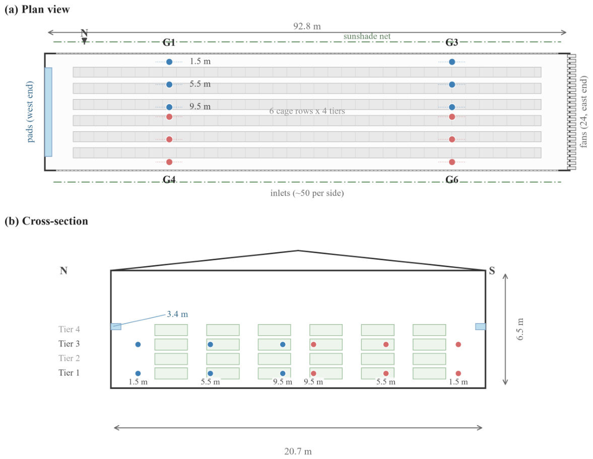
The experiment was conducted in a commercial stacked-cage broiler house in Jilin Province, China (${44}^{°}{50}^{\prime }$23.${60}^{″}$ N, ${126}^{°}{31}^{\prime }$58.${80}^{″}$ E) from 17 February to 24 March 2023. The house measured 92.8 m × 20.7 m × 6.5 m and housed 78,000 broilers in six rows of four tiers. Ventilation was supplied through side-wall inlets on both long walls (about 50 per sidewall) and exhausted by end-wall fans; evaporative cooling pads at the west end were closed in winter, and sunshade nets covered both long walls. Heating was supplied by a heat-exchanger system, and both the inlets and the heaters were commanded by the house climate controller.

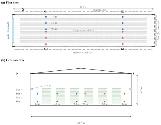
Indoor temperature was recorded by 24 in-cage temperature loggers (HOBO Pro v2, Onset Computer Corp., Bourne, MA, USA; accuracy ±0.2 K) arranged in four of the farm’s inlet groups (Groups 1 and 3 on the north sidewall; Groups 4 and 6 at the analogous longitudinal positions on the south sidewall), each group with three measurement positions at 1.5, 5.5, and 9.5 m from the sidewall and two cage tiers (Tier 1 at 0.5 m and Tier 3 at 2.1 m above the floor). The mean of the loggers defines the indoor temperature series analysed throughout this paper, and their deployment is shown in Figure 1. The in-cage loggers recorded at 1 min resolution and were aggregated to a 5 min record; the outdoor weather station (air temperature, relative humidity, wind speed) logged at 15 min resolution, and the controller channels (damper position, negative pressure, ${\mathrm{CO}}_2$ concentration, and heater contactor state) at about 10 min resolution. Table 1 summarises the measured variables. Instrumentation followed standard guidance for livestock-house environmental monitoring, as compiled in reference handbooks [47,48] and applied in field studies of indoor air quality [36] and IoT-based monitoring [49].

Figure 1. Monitored house and sensor deployment. (a) Plan view: six cage rows, side-wall inlets on both long walls, evaporative cooling pads at the west end and exhaust fans on the east end wall, with sunshade nets over both walls; circles mark the twelve measurement positions of the four inlet groups. (b) Cross-section (north on the left): each position is instrumented at two cage tiers, giving 4 groups × 3 positions × 2 tiers = 24 loggers. The drawing is schematic.

Table 1. Measured variables on the common 15 min grid (3408 records).

Variable	Source	Recorded Resolution	Range	Mean
Indoor temperature (°C)	24 in-cage loggers (HOBO Pro v2)	1 min	21.4 to 33.4	28.3
Outdoor temperature (°C)	weather station	15 min	$-19.2$ to 16.4	$-1.3$
Relative humidity (%)	weather station	15 min	22.8 to 99.8	68.2
Wind speed (m/s)	weather station	15 min	0 to 13.6	3.6
Damper position (%)	climate controller	≈10 min	0.1 to 17.2	4.5 a
Negative pressure (Pa)	climate controller	≈10 min	0 to 83	28.0
${\mathrm{CO}}_2$ concentration (ppm)	climate controller (building-level)	≈10 min	2062 to 4973	3493
Heater contactor state	climate controller	≈10 min	0 (off) to 1 (on)	0.19 b

^a The damper distribution is skewed; its median (4.0%) enters the ventilation cross-checks of Section 2.5. ^b Mean fraction of 15 min records with either contactor closed.

Feeding and lighting followed the farm’s own schedules and were not manipulated for this study. Feed was delivered three times daily, with ad libitum access between deliveries [1]. Lighting followed the age-indexed dark-period programme of the house controller and therefore changed with bird age across the window: at ages 6–28 (most of the study), the lights were off from 11:00 to 14:00 and from 19:00 to 21:00 at a minimum intensity of 5 lx; the midday dark period shortened over ages 29–31 and was removed from age 32, while the evening dark period remained 2 h until it shortened to 1 h from age 35. Because neither schedule was manipulated, the feature set carries no time-of-day or feeding covariate; any circadian component enters the models through the measured drivers and their recent history.

Table 1 lists the measured variables with their ranges and means; indoor temperature ranged from 21.4 to 33.4 °C and outdoor temperature from $-19.2$ to 16.4 °C. All loggers were factory-calibrated units used as delivered, and their readings were analysed as logged, without post hoc correction; the controller channels are the climate controller’s own sensors, and the ${\mathrm{CO}}_2$ channel in particular was not independently calibrated in this campaign, so it is used only as building-level context. No outlier removal was required: all in-cage values fell within 18.9–34.9 °C, inside the physical range expected for a broiler house, and the only quality-control step that modified the record was gap filling.

Missing values were concentrated in a few loggers: of the 24 channels, one returned no data over the whole window and six had 22–64% missing values, whereas the remaining seventeen had less than 0.3% missing. On the 15 min grid, 21 loggers were valid in the median bin (never all 24), and three bins had no valid data at all. All series were aligned to a common 15 min grid by block averaging, and gaps were closed per logger (forward fill followed by linear interpolation) before the house mean was formed, so that the mean always combines the same set of positions. This construction does not drive the results: excluding the six long-gap channels, or omitting gap filling altogether, moves the 15 min persistence floor from 0.105 K to 0.120–0.123 K and the fitted fluctuation amplitude from 0.68 to 0.78 K, while the fitted time constant stays within 25.1–26.2 h (Section 3.2). The alignment yielded 3408 records, of which the last 680 form the test segment (Section 2.2). Absolute temperatures and setpoints are reported in °C; temperature differences and error metrics (root-mean-square error, RMSE; mean absolute error, MAE; $\sigma$; and interval widths) are reported in K, the two being numerically identical for differences.

2.2. Forecasting Task and Features

The target was the 15 min indoor temperature change, $\Delta T\left(t\right)=T\left(t\right)-T(t-1)$, where $T\left(t\right)$ is the house-mean indoor temperature. Predicting the change rather than the absolute level measures model skill on the unpredictable component, not on the autocorrelation that a trivial baseline already captures. All models used exogenous features only: outdoor temperature, humidity, wind speed, ventilation damper position, negative pressure, ${\mathrm{CO}}_2$, and heater state, each taken over a 12-step (3 h) context window ending at the forecast origin. Data were split chronologically into 80% training (17 February–17 March) and 20% test (17–24 March); the feature scaler was fitted on the training segment only. All models were trained on the same split, so differences are attributable to the model family alone. Accuracy is reported as the RMSE of the predicted temperature level over the 680 test windows; for a one-step-ahead forecast this is identical to the RMSE of the 15 min temperature change, which is why the persistence baseline has a non-zero RMSE (0.1046 K) at this horizon.

2.3. Prediction Models

Eighteen single-step models were evaluated. The reference was a persistence baseline ($\Delta \widehat{T}=0$, i.e., for the temperature level, the forecast is simply the last observed value) [20]. Eleven statistical and machine learning models (linear regression, ridge, lasso, elastic net, random forest [15], XGBoost [14], LightGBM, SVR, k-NN, autoregressive integrated moving average, ARIMA [13], and its seasonal variant, SARIMA) were trained on flattened 84-dimensional windows, and six deep learning models (long short-term memory, LSTM [16]; gated recurrent unit, GRU; Transformer [17]; LSTM with attention; temporal convolutional network, TCN [18]; and N-BEATS [19]) on 3-D windows (12 × 7). Deep models used two recurrent layers with a hidden size of 128 (LSTM, GRU, LSTM with attention), a Transformer with $d_{\mathrm{model}}=64$ and four attention heads, a temporal convolutional network with 64 channels over three layers, and N-BEATS with three blocks. Dropout was 0.1–0.2; the optimiser was Adam with learning rate ${10}^{-3}$, batch size 64, and mean-squared-error loss; and early stopping was applied on a validation split (patience 10). Each model was trained five times from different random initialisations, and the run-to-run RMSE variability is reported. In addition, three physics-based variants of a lumped-capacitance thermal balance model were evaluated (Section 2.5).

2.4. Multi-Horizon Forecasting

For horizons of 1, 4, 8, 24, and 48 h (4–192 steps), dedicated direct-forecasting models were trained on the residual $r_h\left(t\right)=T(t+h)-T\left(t\right)$, using the same 12-step context window; predictions were reconstructed as $\widehat{T}(t+h)=T\left(t\right)+{\widehat{r}}_h$. LSTM and linear regression were compared with the persistence forecast $\widehat{T}(t+h)=T\left(t\right)$ on the identical chronological split.

2.5. Thermal Time Constant and Multi-Scale Analysis

For a first-order lumped system, the persistence error at horizon $\Delta t$ satisfies

$${\mathrm{RMSE}}^2(\Delta t)=2{\sigma }^2\left[1-\exp (-\Delta t/\tau )\right]$$

(1)

where $\sigma$ is the amplitude of temperature fluctuation about the local equilibrium. $\tau$ and $\sigma$ were estimated by nonlinear least squares over the six measured horizons (15 min–48 h); the uncertainty of $\tau$ was quantified by residual bootstrap of the six-point fit (300 resamples). Multi-scale structure was assessed with the autocorrelation function (ACF). A single-exponential model, $\mathrm{ACF}\left(l\right)=\exp (-l\Delta t/\tau )$, was compared with a double-exponential model, $a\exp (-l\Delta t/{\tau }_f)+(1-a)\exp (-l\Delta t/{\tau }_s)$, by AIC; the effective $\tau$ inferred from the ACF at selected lags was computed to show scale dependence. Fit uncertainty of the ACF parameters was quantified by lag-domain residual block bootstrap (block 24 lags, 300 resamples); because these intervals are conditional on the fitted curve, the identifiability of the slow scale within the 35-day record was additionally checked with a sequence block bootstrap (block 96 steps = 24 h, 150 resamples).

The ventilation dependence of $\tau$ was derived from the calibrated physical model [7,8,9], following the dynamic thermal-load approach of [10]. The analytical (exact) relaxation step of the lumped model is

$$T(t+\Delta t)=T_{\mathrm{eq}}+\left[T\left(t\right)-T_{\mathrm{eq}}\right]\exp (-\Delta t/\tau \left(t\right))$$

(2)

where the local equilibrium temperature and the time constant are

$$T_{\mathrm{eq}}=T_{\mathrm{out}}+{\displaystyle \frac{Q_{\mathrm{birds}}+Q_{\mathrm{heater}}}{G\left(t\right)}},\tau \left(t\right)={\displaystyle \frac{C_{\mathrm{eff}}}{G\left(t\right)}}$$

(3)

and the total conductance (envelope plus ventilation) and the effective heat capacity are

$$G\left(t\right)=G_{\mathrm{env}}+\rho C_p\left[v_{\mathrm{base}}+k_{\mathrm{vent}}q\left(t\right)\right],C_{\mathrm{eff}}=\rho V{C}_p{c}_{\mathrm{eff}}$$

(4)

with $T_{\mathrm{out}}$ being the outdoor temperature, $q\left(t\right)$ the damper position, $G_{\mathrm{env}}$ the envelope conductance, and $c_{\mathrm{eff}}$ a dimensionless multiplier of the air-volume heat capacity.

The four uncertain parameters (heat per bird, effective capacity, ventilation-flow scaling, and heater power) were calibrated by grid search on the training segment. The grid covered heat per bird over 8, 16, 24, and 32 W, which is 0.6–2.5 MW in total for the 78,000 birds housed; $c_{\mathrm{eff}}$ over four geometric values from 50 to 400; ventilation scaling over 500, 1750, and $3000 {\mathrm{m}}^3$/s per unit damper fraction; and heater power over 0.30, 0.65, and 1.00 MW, giving 144 configurations. The selected configuration supplied 1.25 MW of bird heat (16 W per bird, an effective input that also absorbs unmodelled in-house gains such as lighting and litter fermentation), with $c_{\mathrm{eff}}$ = 400, ventilation scaling 500 ${\mathrm{m}}^3$/s per unit damper fraction, and 0.30 MW of heater power; it reproduced the training-segment temperatures with RMSE 5.2 K. The RMSE surface over the grid is smooth, and the selected configuration is separated from the next-ranked configuration by 0.7 K (the five best configurations span 5.2–7.9 K), so the effective parameter values are resolved to within the granularity of the grid. The uncalibrated variant used literature defaults [47,48], and a controller variant emulated thermostat logic (ventilation boost when $T>T_{\mathrm{set}}$, reduction when $T<T_{\mathrm{set}}-2$ K).

The two parameters that govern the dynamics have direct physical interpretations, and both can be cross-checked independently of the calibration objective. The value $c_{\mathrm{eff}}=400$ corresponds to a lumped heat capacity of about 6.0 GJ/K, that is, 400 times the heat capacity of the house air (15.1 MJ/K for 12,500 ${\mathrm{m}}^3$). This is equivalent to a concrete slab roughly 1.5 m thick over the floor area: the effective mass stands for the floor, the litter, the building fabric, and the birds, and it also absorbs the unmodelled in-house gains. At the median damper position (4%), Equations (3) and (4) then give $\tau \approx$ 34 h. That value is of the same order as the time constant estimated from persistence growth ($\tau =25.7$ h; 95% CI [10.5, 153.9] h; Section 3.2), which is obtained directly from the record and never enters the calibration.

The ventilation scaling is consistent with the farm’s own design specification. The installed fans are rated at 1,000,000 ${\mathrm{m}}^3$/h (278 ${\mathrm{m}}^3$/s) in total. The calibrated mapping gives 20 + 500 × 0.172 ≈ 106 ${\mathrm{m}}^3$/s at the highest damper position observed (17.2%), of which 86 ${\mathrm{m}}^3$/s comes from the damper term and 20 ${\mathrm{m}}^3$/s from the minimum-fan flow. That is about 38% of the installed capacity, close to the design maximum-ventilation setting of 30% at the end of the cycle; at the median damper, the mapped flow is 40 ${\mathrm{m}}^3$/s, or 1.8 ${\mathrm{m}}^3$/h per bird. The mapping is used only over the observed damper range, is not extrapolated to full opening, and follows the orifice behaviour documented for sidewall inlets [27,28,50]. A ${\mathrm{CO}}_2$ mass balance provides a further check: the mean mapped flow (42 ${\mathrm{m}}^3$/s) and the mean ${\mathrm{CO}}_2$ concentration (3493 ppm against an outdoor background of about 420 ppm) together imply a whole-house ${\mathrm{CO}}_2$ production of about 6 L/h per bird. That is the same order as the broiler ${\mathrm{CO}}_2$ output reported for ventilation-flow balances (3.7 L/h per kg of metabolic weight, plus about one fifth from the litter [51]). Equation (2) supplies both the environment stepped forward in the control simulation (Section 2.7) and the ventilation dependence of $\tau$ reported in Section 3.2.

2.6. Probabilistic Forecasting

For horizons of 15 min and 1, 4, and 24 h, XGBoost quantile regressors ($\alpha =0.05$ and $0.95$, pinball loss) [52] predicted the residual quantiles from the last context step. Reconstructing the level gives the empirical 90% band $[T\left(t\right)+q_{0.05},T\left(t\right)+q_{0.95}]$. Coverage was measured by the prediction interval coverage probability (PICP) [46] on the training (in-sample) and test (out-of-sample) segments. As a theoretical alternative, a Gaussian band centred on the persistence forecast was evaluated on the same points, with the standard deviation of the h-step persistence error given by

$$\sigma \left(h\right)=\sqrt{2{\sigma }^2\left[1-\exp (-h\Delta t/\tau )\right]}$$

(5)

so that the band is $T\left(t\right)\pm 1.96\sigma \left(h\right)$. To balance coverage against sharpness, both bands were also scored with the interval score [45]

$$\mathrm{IS}=⟨(u-l)+{\displaystyle \frac{2}{\alpha }}(l-y)\mathbf{1}(y<l)+{\displaystyle \frac{2}{\alpha }}(y-u)\mathbf{1}(y>u)⟩$$

(6)

where, in Equation (6), $[l,u]$ is the predicted interval, and $\alpha =0.1$ for the 90% band. The interval score rewards narrow intervals and penalises misses, so a wider but better-calibrated band can still score better.

2.7. Counterfactual Control Simulation

A counterfactual simulation compared four ventilation strategies in the calibrated analytical environment of Equation (2), driven by the measured outdoor-temperature record [53], with ventilation rates mapped through balance methods [39] and opening discharge coefficients [41,42]. The strategies were: (i) replay of the measured damper and heater actions, as an environment sanity check; (ii) proportional feedback control, with the damper proportional to the temperature error and clipped to 0.1–20%; (iii) rolling-horizon MPC re-optimised every hour from a piecewise-constant control sequence (a near-term 1 h piece plus a constant remainder), evaluated at horizons of 1, 4, 8, 24, and 48 h; and (iv) a robustness assessment of the environment model itself, in which each calibrated parameter was perturbed by ±20% and structural mismatch was probed by adding process noise ($\sigma$ = 0.25–1.0 K) or bias (±1 K) to the executed environment while the controller kept the noise-free model (Section 3.6). Both assessments cover the 1, 4, 8, and 24 h horizons, so that the recommended preview window is tested alongside the short and long alternatives. The ±20% range brackets the uncertainty of each calibrated parameter: the effective capacity and the ventilation scaling are effective quantities resolved only to the granularity of the calibration grid (Section 2.5), and the bird heat input carries the uncertainty of the metabolic-rate estimate. All MPC variants minimised the same cost $\sum {\left(T-T_{\mathrm{set}}\right)}^2+\lambda u^2$ ($\lambda =0.02$, setpoint 27.5 °C) under identical action-cost constraints; the heater followed a hysteresis rule (on below 27 °C, off above 29 °C). Metrics comprised temperature standard deviation ${\sigma }_T$, mean absolute deviation from setpoint, ventilation/heating energy (ventilation heat removed plus heater energy), and the number of events outside 24–33 °C.

2.8. Statistical Analysis

Differences against the persistence baseline were tested with the Diebold–Mariano test [21] on squared errors with Newey–West (HAC) variance correction, at each model–horizon combination. Multiple testing across the 27 combinations was controlled with the Benjamini–Hochberg false-discovery-rate (FDR) procedure (q < 0.05). The multi-horizon LSTM was trained three times, and the range of the Diebold–Mariano p-value across runs is reported to bound the stability of significance. Deep learning stability at the 15 min horizon was quantified by five repeated trainings. Feature importance was assessed by Shapley additive explanations (SHAP) values [54] for an XGBoost model trained on the identical 15 min residual task, using the last context step. Extreme-event classification (indoor temperature above the 90th percentile or $\mathrm{mean}+1\sigma$ of each training fold) was attempted with time-series cross-validation; thresholds were computed on training folds only. All analyses were performed in Python 3.13.12 with NumPy 2.4.6, pandas 3.0.5, scikit-learn 1.9.0, SciPy 1.18.0, statsmodels 0.14.6, XGBoost 3.3.0, LightGBM 4.7.0, SHAP 0.52.0, and PyTorch 2.13.0 (CUDA 13.2), and the figures were produced with Matplotlib 3.11.1. The NumPy and scikit-learn seeds are fixed (42), the PyTorch seed is fixed per repeat (42 plus the repeat index), and the bootstrap and control-simulation seeds are 0–2; deep-learning metrics are averages over the repeated trainings, with the run-to-run variability reported alongside.

3. Results

3.1. Single-Step Performance: Convergence to the Persistence Baseline

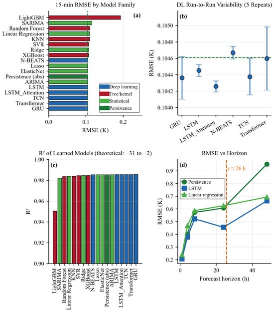
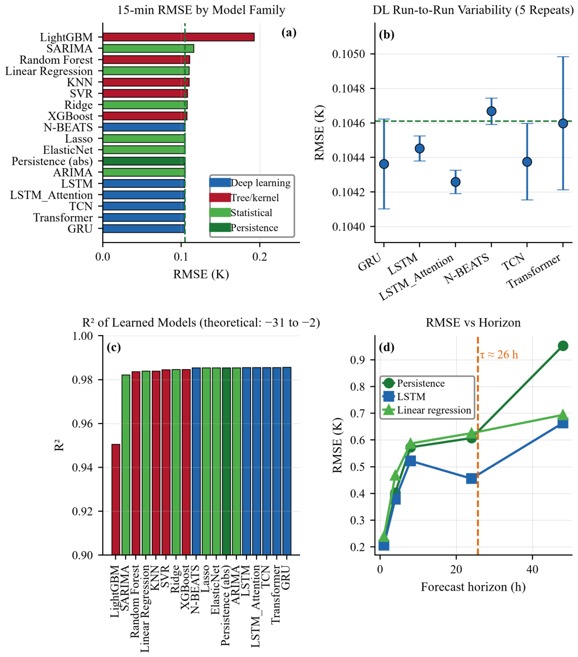
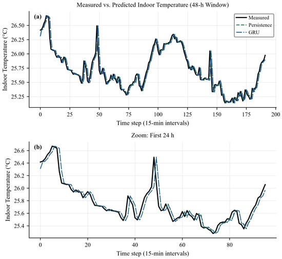
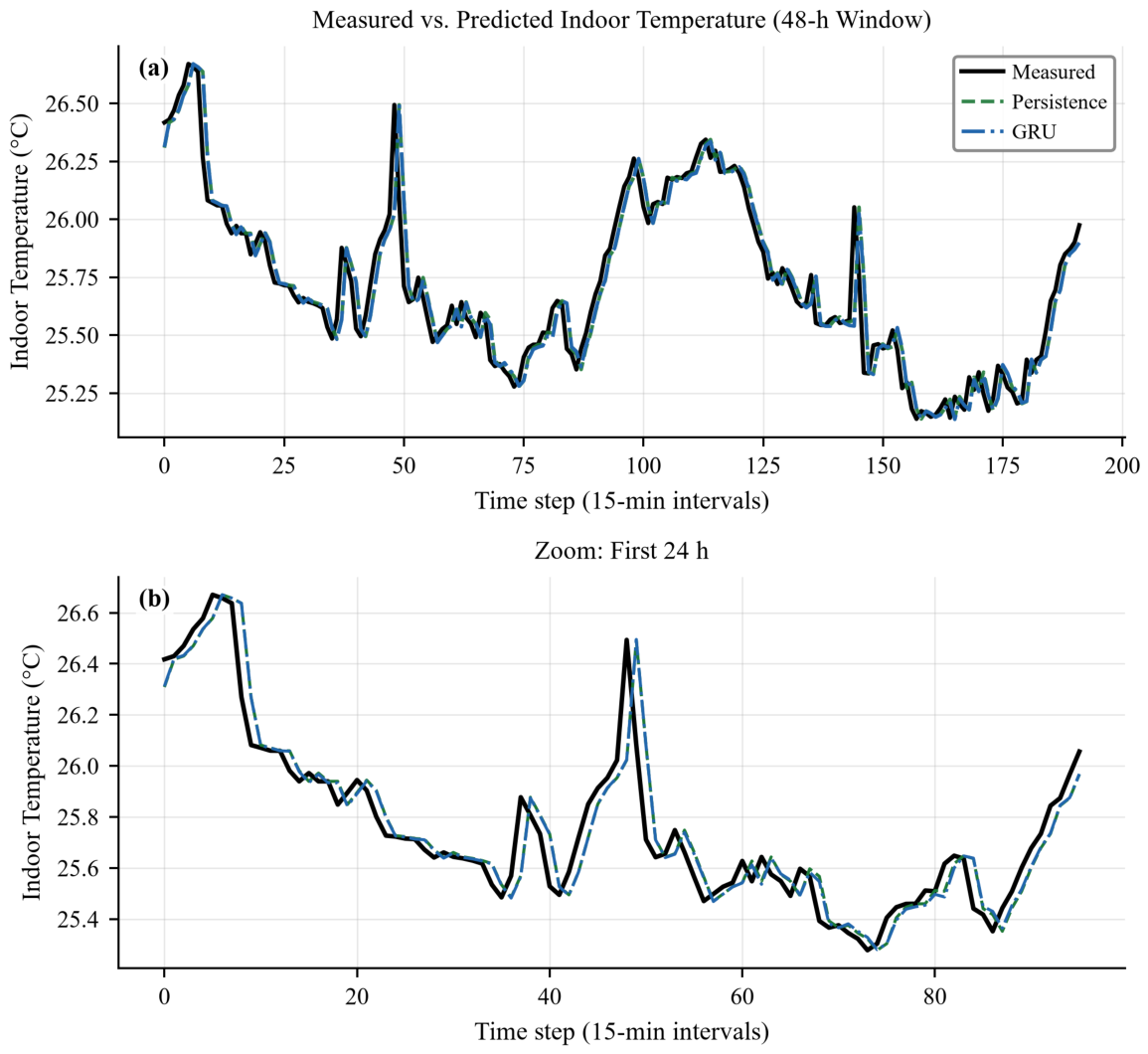
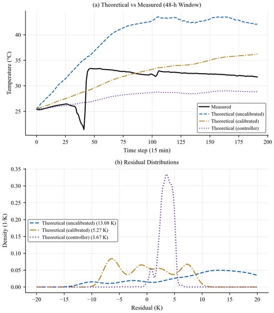
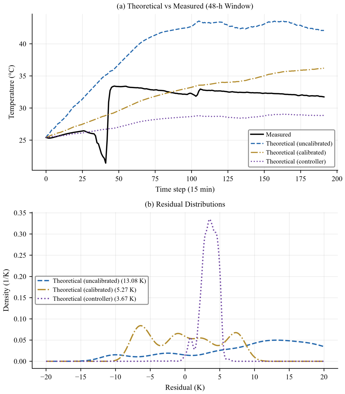
At 15 min resolution, most learned single-step models converged to the persistence baseline (RMSE = 0.1046 K, ${\mathrm{R}}^2$ = 0.9855; Table 2, Figure 2a): 9 of the 17 learned models matched it to within 0.001 K, whereas tree ensembles and SARIMA were worse (0.107–0.193 K), and significantly so for five combinations (Section 3.3). The best models were deep networks (GRU 0.1040 K; Transformer, TCN, and LSTM with attention 0.1042 K; LSTM 0.1043 K), followed by ARIMA and regularised linear models (0.1046 K). Run-to-run variability across five repeated trainings was negligible (LSTM 0.1045 ± 0.0001 K), so the convergence to persistence is not an artefact of a single run (Figure 2b). The time series of measured and predicted temperature are visually indistinguishable at this horizon (Figure 3), and the residual distributions of the top models are near-identical and near-Gaussian. The plotted window spans 192 consecutive 15 min samples (48 h) of the test segment, over which the house mean varies by only 1.5 K, and the 24 h zoom by 1.4 K; this narrow range, the signature of a controller holding the house near its setpoint, is why every model returns the persistence forecast at this horizon. All RMSE differences among the top models and the persistence baseline are below 0.001 K, far smaller than the ±0.2–0.5 K accuracy of typical air-temperature sensors. At this horizon, the top models are therefore operationally equivalent to persistence. The theoretical thermal-balance models did not reproduce the measured temperatures (RMSE 3.7–13.1 K; ${\mathrm{R}}^2$ < 0), because the house temperature is set by the ventilation controller rather than by passive thermal balance alone (Figure 4).

Table 2. Single-step model performance on the test set (15 min resolution), ranked by RMSE.

Model	RMSE (K)	MAE (K)	${\mathrm{R}}^2$	MAPE (%)	Max Error (K)
GRU a	0.1040	0.0692	0.9856	0.27	0.6190
Transformer a	0.1042	0.0697	0.9856	0.28	0.6102
TCN a	0.1042	0.0693	0.9856	0.28	0.6168
LSTM_Attention a	0.1042	0.0697	0.9856	0.28	0.6103
LSTM a	0.1043	0.0693	0.9855	0.28	0.6183
ARIMA	0.1046	0.0697	0.9855	0.28	0.6127
Persistence	0.1046	0.0694	0.9855	0.28	0.6172
ElasticNet	0.1046	0.0694	0.9855	0.28	0.6175
Lasso	0.1046	0.0694	0.9855	0.28	0.6175
N-BEATS a	0.1046	0.0696	0.9854	0.28	0.6161
XGBoost	0.1073	0.0746	0.9847	0.30	0.6062
Ridge	0.1074	0.0766	0.9847	0.30	0.5600
SVR	0.1080	0.0764	0.9845	0.30	0.6365
KNN	0.1100	0.0768	0.9839	0.30	0.5726
Linear Regression	0.1100	0.0823	0.9839	0.33	0.5476
Random Forest	0.1108	0.0747	0.9837	0.30	0.6403
SARIMA	0.1158	0.0849	0.9822	0.34	0.5398
LightGBM	0.1929	0.1253	0.9505	0.50	0.8484

^a DL models trained 5×; run-to-run RMSE SD ≤ 0.001 K (e.g., LSTM 0.1045 ± 0.0001). Test set: 680 windows of 15 min data; one-step-ahead RMSE is evaluated on the temperature level, which at this horizon is identical to the RMSE of the 15 min temperature change (Section 2.2).

Figure 2. Model benchmark and horizon trend. (a) Test-set RMSE of the 17 learned single-step models and the persistence baseline at 15 min resolution, coloured by model family (vertical dashed line: persistence); (b) run-to-run RMSE of the six deep learning models over five repeated trainings (error bars: ±1 SD; dashed line: persistence baseline, RMSE = 0.1046 K); (c) ${\mathrm{R}}^2$ of the same learned models; (d) RMSE growth with forecast horizon for persistence, LSTM, and linear regression (1–48 h), with the estimated $\tau$ = 25.7 h marked.

Figure 3. Measured vs. predicted indoor temperature: (a) 192 consecutive 15 min samples (48 h) from the test segment, showing the measured series with the persistence and GRU predictions; (b) 96-sample zoom (24 h) of the same series.

Figure 4. Theoretical thermal-balance model variants vs. measured temperature: (a) 48 h trajectories of the uncalibrated, calibrated, and controller-enhanced analytical models; (b) residual distributions with RMSE values annotated.

3.2. Thermal Time Constant and Multi-Scale Dynamics

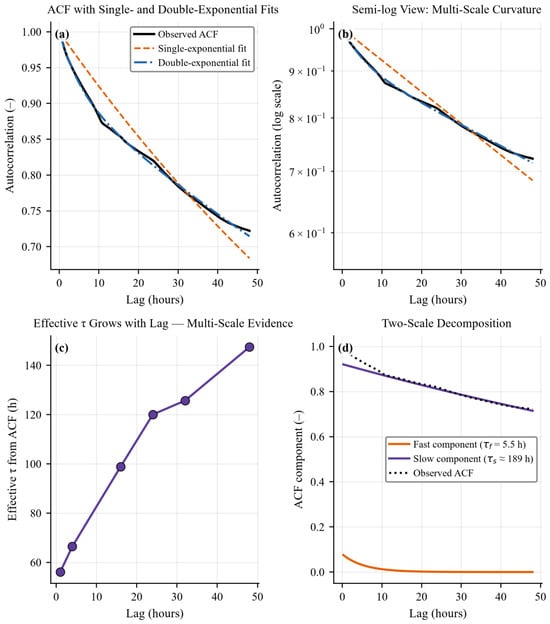
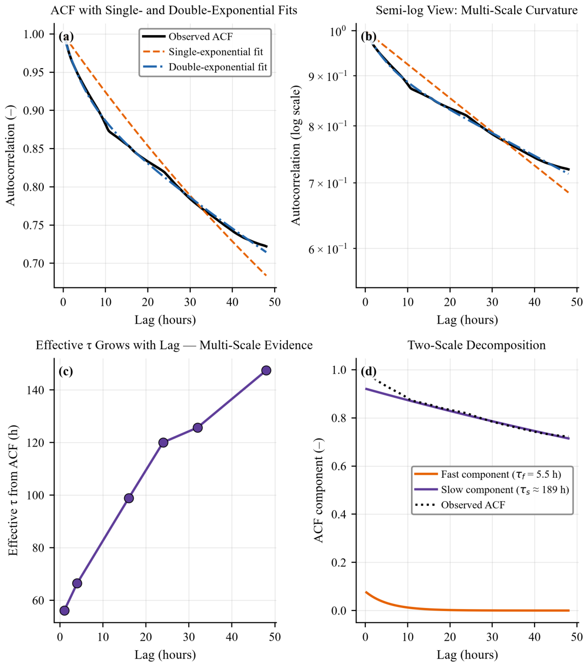
Fitting Equation (1) to the six persistence errors (15 min: 0.1046 K; 1 h: 0.2082 K; 4 h: 0.4030 K; 8 h: 0.5727 K; 24 h: 0.6071 K; 48 h: 0.9529 K) yielded $\tau =25.7\pm 15.7$ h and $\sigma =0.68$ K (Table 3). The fit residual is non-zero because the system is not single-exponential. The ACF is overwhelmingly better described by a double exponential ($\Delta \mathrm{AIC}=-763$) with a fast scale (${\tau }_f=5.5$ h) carrying 8% of the variance and a slow scale (${\tau }_s\approx 189$ h) carrying 92% (Figure 5a,b,d). Accordingly, the effective $\tau$ inferred from the ACF grows with lag (56 h at 1 h, 66 h at 4 h, 99 h at 16 h, 120 h at 24 h, and 147 h at 48 h; Figure 5c), so longer horizons are governed by progressively slower dynamics.

Table 3. Thermal time constant estimation and multi-scale decomposition.

Quantity	Value
RMSE(15 min)/1 h/4 h/8 h/24 h/48 h (persistence, K)	0.1046/0.2082/0.4030/0.5727/0.6071/0.9529
$\tau$ (Equation (1) fit, h)	25.7 ± 15.7
$\tau$ 95% CI (residual bootstrap, h)	[10.5, 153.9]
$\sigma$ (Equation (1) fit, K)	0.68
ACF single-exponential $\tau$ (h)	126.3
ACF double-exponential: ${\tau }_f$ (h), variance share	5.5 h, 8%
ACF double-exponential: ${\tau }_s$ (h), variance share	189 h, 92%
ACF parameters 95% CI (residual block bootstrap)	${\tau }_f$ [5.1, 5.9] h; a [0.07, 0.08]; ${\tau }_s$ [184.7, 193.9] h
${\tau }_s$ 95% range (sequence block bootstrap, h)	10–1543
$\Delta$AIC (double−single)	−763
Effective $\tau$ from ACF: 1/4/16/24 h lag (h)	56/66/99/120
Physical $\tau \left(q\right)$: 0.7% to 8.6% damper (h)	56.6 to 21.7

Figure 5. Multi-scale thermal dynamics, computed on the full 35-day record (3408 records at 15 min resolution). (a) Autocorrelation function with single- and double-exponential fits; (b) semi-log view of the same curves; (c) effective $\tau$ inferred from the ACF at increasing lags; (d) decomposition into a fast (${\tau }_f$) and a slow (${\tau }_s$) component.

Bootstrap resampling quantifies the uncertainty of these estimates (Table 3). Residual bootstrap of the six-point fit gives a wide 95% CI of [10.5, 153.9] h for $\tau$: six horizons carry limited information, and the right tail is poorly constrained by the 48 h point. The ACF parameters are tightly identified conditional on the two-exponential model (95% CI: ${\tau }_f$ [5.1, 5.9] h, a [0.07, 0.08], ${\tau }_s$ [184.7, 193.9] h), but the slow scale is only partially identifiable within a 35-day record. The ACF decays by less than 30% over the maximum explored lag (48 h), and a sequence block bootstrap yields a 10–1543 h range for ${\tau }_s$. The slow scale should therefore be read as an order-of-magnitude estimate whose confirmation requires a longer record.

A practical estimator based on a short record was also probed, by fitting the ACF initial decay (lags up to 4 h) on every window of a given length across the record (Table 4). The estimate converges from below as the window grows: the median ${\tau }_f$ is 1.3 h for 12 h windows (interquartile range 0.9–2.0 h), 2.8 h for 24 h windows, 4.3 h for 48 h windows, and 5.3 h for 72 h windows, against 5.5 h for the full record. The practical implication is that the fast scale can be estimated from a record of about three days: the resulting control preview (0.7–1.5 ${\tau }_f$) is 2–4 h from a one-day record and 4–8 h from a three-day record, converging on the recommendation of Section 4.3; shorter windows capture only the fastest part of the response. The slow scale needs multi-day records. The scale of interest must therefore be selected deliberately: ${\tau }_f$ for control preview (Section 3.6), the lumped $\tau$ for forecast-skill horizons (Section 3.3), and ${\tau }_s$ for multi-day planning.

Table 4. Short-record estimation of the fast scale: ACF initial decay (lags up to 4 h) fitted on windows of increasing length ^a.

Estimation Window	Windows	Median ${\mathit{\tau }}_{\mathit{f}}$ (h)	Interquartile Range (h)	Implied Preview 0.7–1.5 ${\mathit{\tau }}_{\mathit{f}}$ (h)	Ratio to Full-Record ${\mathit{\tau }}_{\mathit{f}}$
12 h	71	1.3	0.9–2.0	0.9–1.9	0.23
24 h	70	2.8	1.4–3.6	2.0–4.2	0.52
48 h	68	4.3	2.8–6.2	3.0–6.4	0.78
72 h	66	5.3	3.5–9.0	3.7–7.9	0.96
Full record (35 days)	1	5.5	—	3.9–8.2	1.00

^a Windows start on a 12 h grid. The full-record value is the fast scale of the bi-exponential ACF (Table 3).

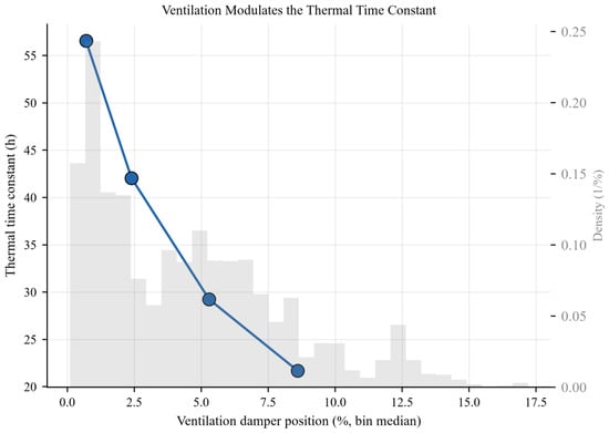
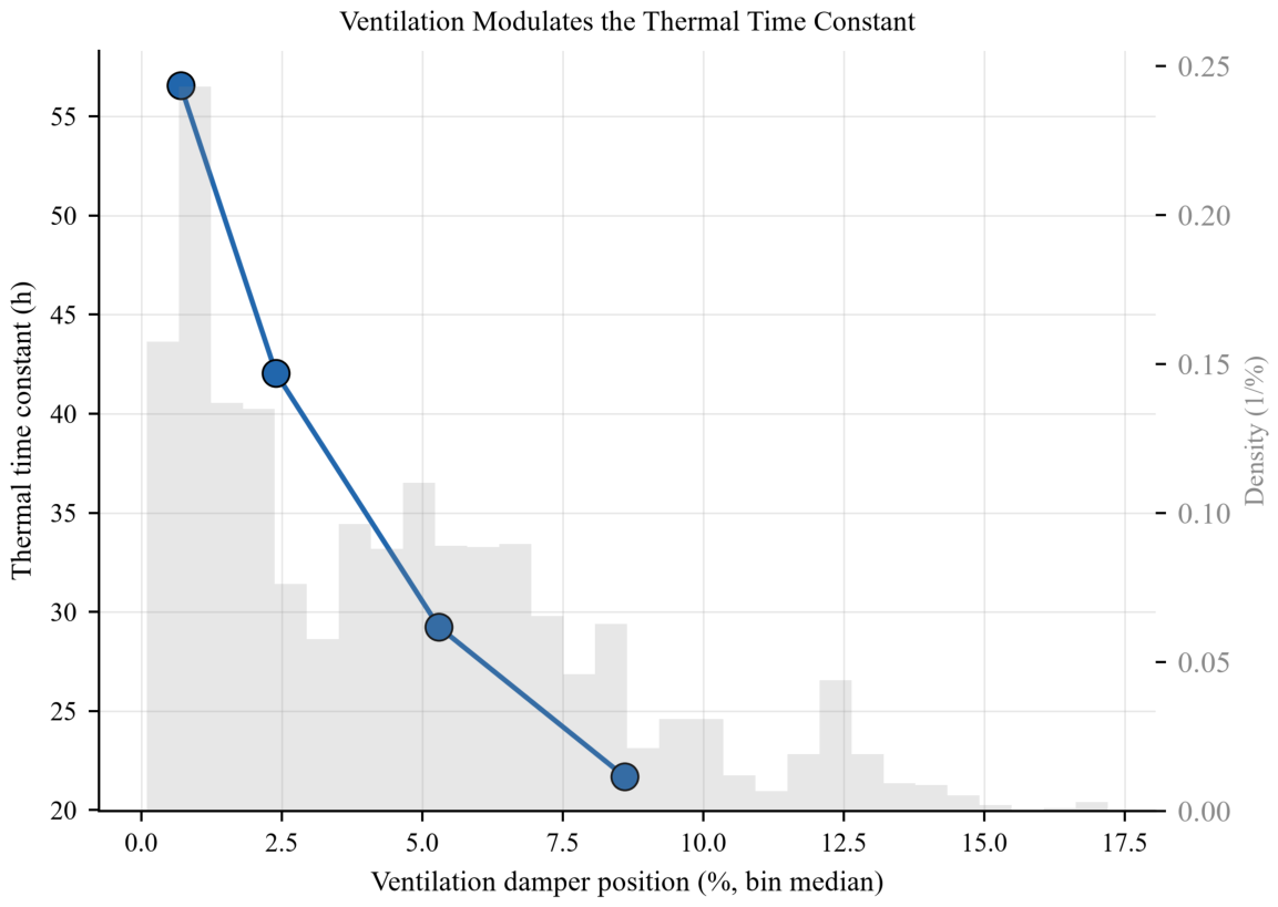
The physical model predicts that the damper actively tunes $\tau$: raising the damper position from 0.7% to 8.6% increases conductance and reduces the time constant from 56.6 to 21.7 h (Figure 6). In the calibrated model, the ventilation controller therefore not only regulates temperature; it also modulates the very time constant that determines predictability.

Figure 6. Ventilation modulates the thermal time constant. Calibrated-model prediction of $\tau \left(q\right)$ = $C_{\mathrm{eff}}/G\left(q\right)$ across the observed damper range, with the measured damper-position distribution in the background.

3.3. Multi-Horizon Forecasting and Statistical Robustness

Dedicated direct-forecasting models were compared with persistence at five horizons (Table 5, Figure 2d). At 1 h, neither LSTM (0.207 K) nor linear regression (0.239 K) reliably beat persistence (0.208 K). The LSTM advantage grew steadily with horizon (−1% at 1 h, −6% at 4 h, −9% at 8 h, −25% at 24 h, and −30% at 48 h; RMSE 0.379, 0.522, 0.455, and 0.664 K versus persistence 0.403, 0.573, 0.607, and 0.953 K). The LSTM forecast is the mean of three trained networks; the corresponding mean single-run RMSEs are 0.207, 0.382, 0.524, 0.593, and 0.670 K, so the averaging is what produces the 24 h gain (Table 5). Linear regression remained at or above persistence until 48 h (−27%). The RMSE gain is stable across repeated trainings at 4–48 h except at 24 h, where run-to-run variability is large (SD 0.13 K); what varies between training runs is mainly the statistical significance at short-to-intermediate horizons (see below). The persistence floor is therefore real but bounded: models escape it when the horizon becomes commensurate with the thermal time constant.

Table 5. Direct multi-horizon forecasting (test set): persistence, LSTM (mean of three trainings), and linear regression.

Horizon	Steps (15 min)	Persistence RMSE (K)	LSTM RMSE (K)	LSTM Run-to-Run RMSE (Mean ± SD, K)	LSTM DM p-Range (3 Runs) a	Linear Regression RMSE (K)
1 h	4	0.2082	0.2067	0.2068 ± 0.0004	0.030–0.212	0.2392
4 h	16	0.4030	0.3786	0.3817 ± 0.0080	0.010–0.119	0.4680
8 h	32	0.5727	0.5220	0.5237 ± 0.0092	0.005–0.146	0.5868
24 h	96	0.6071	0.4554	0.5929 ± 0.1306	<0.001–0.050	0.6256
48 h	192	0.9529	0.6636	0.6697 ± 0.0160	<0.001–0.001	0.6938

^a LSTM vs. persistence (mean prediction, i.e., the average of the three trained networks): 1 h −1% (ns); 4 h −6%; 8 h −9%; 24 h −25%; 48 h −30%. Run-to-run RMSE SD is ≤0.016 K at 4–48 h except at 24 h (0.13 K). DM p-range = Diebold–Mariano p-value across the three repeated trainings of the final campaign; across four independent campaigns, the 48 h gain was significant in every run (p ≤ 0.0025), as was the 24 h gain in every run of three campaigns (worst p = 0.174), while 4–8 h significance flipped between campaigns (Section 3.3).

Diebold–Mariano tests across 27 model–horizon combinations found 12 combinations significant at p < 0.05, of which 9 survive Benjamini–Hochberg FDR correction for multiple testing (q < 0.05; Table 6). Four are significantly better than persistence: LSTM at 24 h (q = 0.031) and 48 h (q = 0.002), linear regression at 48 h (q = 0.050), and the 15 min TCN (q = 0.039, gain below 0.001 K); the remaining five are significantly worse (tree/kernel baselines at 15 min, linear regression at 1 h).

Table 6. Diebold–Mariano tests vs. persistence (significant at p < 0.05; FDR-corrected q-values).

Model	Horizon	DM Statistic a	p-Value	q-Value (BH-FDR)	RMSE Gain vs. Persistence
SARIMA	15 min	+5.00	<0.001	<0.001	worse
LightGBM	15 min	+4.27	<0.001	<0.001	worse
LSTM	48 h	−3.76	<0.001	0.002	−30%
KNN	15 min	+3.23	0.001	0.008	worse
Linear Regression	1 h	+3.10	0.002	0.010	worse
LSTM	24 h	−2.65	0.008	0.031	−25%
TCN	15 min	−2.53	0.012	0.039	<0.1%
Random Forest	15 min	+2.85	0.004	0.020	worse
Linear Regression	48 h	−2.40	0.017	0.050	−27%

^a Negative DM statistic = model better than persistence; “worse” = significantly worse than persistence. Of 27 combinations, 9 survive Benjamini–Hochberg FDR correction (q < 0.05): 4 better (LSTM at 24/48 h, LR at 48 h, TCN at 15 min) and 5 worse. Multi-horizon LSTM p-value ranges across three repeated trainings are reported in Table 5; across four independent training campaigns, the 48 h gain was significant in every run (p ≤ 0.0025) and the 24 h gain in every run of three campaigns, while 4–8 h significance flipped between campaigns.

Because the multi-horizon LSTM was trained three times per campaign and the full campaign was repeated four times, the stability of significance is itself bounded (Table 5). The 48 h gain was significant in every training run of all four campaigns (p ≤ 0.0025), and the 24 h gain in every run of three campaigns and most runs of the fourth (worst p = 0.174). At 1–8 h, significance flipped between campaigns (for the mean prediction, 1 h was never significant, although individual runs reached p = 0.030; 4–8 h p-ranges of 0.0006–0.016, 0.05–0.91, 0.05–0.20, and 0.005–0.15 across campaigns), even though the RMSE gains of −6% to −9% were stable. Statistical significance at these intermediate horizons is therefore not reproducible, and no model superiority is claimed below 24 h. The statistically robust statements are: gains are real from ≈$\tau /3$ onwards, and significance is reliable from ≈$1\tau$ (24 h) and unconditional at ≈$2\tau$ (48 h). A separate attempt to classify imminent extreme events (temperature above the training-fold 90th percentile or $\mathrm{mean}+1\sigma$; Section 2.8) is not reported further because it could not be evaluated: no test window contained a positive event, with thresholds of about 31–33 °C standing against test maxima of 30.6 °C.

3.4. Probabilistic Forecasting Under Distribution Shift

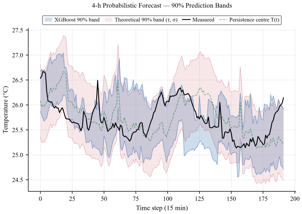
The quantile regressor was well calibrated in-sample (PICP = 0.899–0.903 at all horizons) but under-covered out-of-sample (PICP = 0.607–0.722) (Table 7, Figure 7). This pattern is consistent with a distribution shift: the training period (which includes the February cold spell) is roughly 50% more volatile than the test period (residual $\sigma$ 0.159 K vs. 0.105 K), and the learned conditional quantiles did not adapt. By contrast, the $\tau$-anchored theoretical band (Equation (5)), driven by only two physical parameters, remained well calibrated under the same shift (PICP = 0.923–0.971), and its width grew with horizon in agreement with the measured quantile widths (Figure 7). The interval score, which balances coverage against sharpness, confirms this picture at short horizons: at 15 min–4 h, the theoretical band scores better (IS 0.52–1.71 vs. 0.71–2.79 K) despite being roughly twice as wide, because the quantile band’s under-coverage penalty dominates. At 24 h, the narrower quantile band achieves the lower interval score (2.51 vs. 3.06 K), but only at 0.72 coverage, far below the nominal 0.90, while the theoretical band remains at 0.97. Physical priors transferred where learned intervals failed, at the cost of wider intervals.

Table 7. Probabilistic forecasting: 90% band coverage (PICP), width, and interval score.

Horizon	PICP Train (XGBoost)	PICP Test (XGBoost)	PICP Test (Theoretical) a	Width XGBoost (K)	Width Theoretical (K)	IS XGBoost (K)	IS Theoretical (K)
15 min	0.900	0.607	0.940	0.18	0.37	0.71	0.52
1 h	0.899	0.716	0.923	0.42	0.74	1.20	0.97
4 h	0.899	0.706	0.926	0.93	1.44	2.79	1.71
24 h	0.903	0.722	0.971	1.12	2.95	2.51	3.06

^a Theoretical band: persistence-centred, width $2\times 1.96\sigma \left(h\right)$ from Equation (5), with $\tau =25.7$ h and $\sigma =0.68$ K. Evaluated on the same test segment as the quantile bands: n = 680, 679, 677, and 661 windows at 15 min and 1, 4 and 24 h respectively (n = 2716, 2714, 2704, and 2640 in training). Interval score (IS, $\alpha =0.1$): lower is better; rewards sharpness and penalises misses. IS is better for the theoretical band at 15 min–4 h, and for the quantile band at 24 h where its coverage falls to 0.72.

Figure 7. Probabilistic forecasting at the 4 h horizon: 90% prediction bands from XGBoost quantile regression (blue) and from the $\tau$-anchored theoretical band (red), with the measured temperature and the persistence centre (192 test windows shown).

3.5. Feature Importance

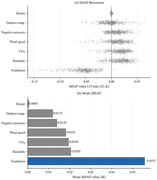
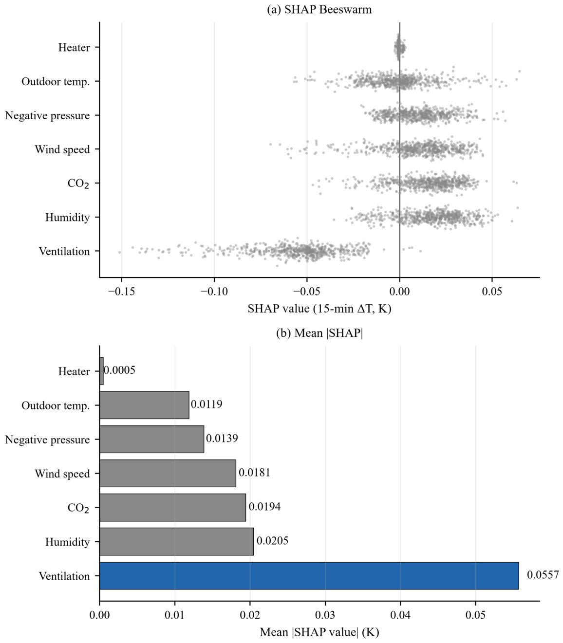
SHAP analysis of the 15 min residual task ranked ventilation damper position first (mean |SHAP| = 0.056 K), followed by humidity (0.020), ${\mathrm{CO}}_2$ (0.019), wind speed (0.018), negative pressure (0.014), and outdoor temperature (0.012); heater state contributed negligibly (0.001) (Figure 8). Ventilation dominates by a factor of ≈5 over outdoor temperature, indicating that the controller’s recent damper actions, rather than the weather, dominate the 15 min residual. This dominance reflects the immediate influence of the controller’s recent damper decisions on the next 15 min temperature change; outdoor temperature acts through those decisions and, in this feedback loop, carries less direct predictive weight.

Figure 8. SHAP feature importance for the 15 min residual task. (a) Beeswarm of SHAP values; (b) mean |SHAP| per feature.

To test whether these contributions survive retraining without a feature group, both a gradient-boosted tree model and the LSTM were re-trained with each group removed in turn, on the 15 min residual task and on the 24 h direct-forecast task (Table 8). At 15 min, removing the ventilation-control group was the only change that degraded the tree model (RMSE 0.107 to 0.134 K); the LSTM was insensitive at this horizon (changes below 0.001 K), consistent with the convergence of all learned models to the persistence floor (Section 3.1). At 24 h, the ventilation-control group remained the dominant input for both models (tree RMSE 0.74 to 1.50 K; LSTM 0.49 to 0.53 K), whereas the remaining groups changed the LSTM’s 24 h RMSE by less than 0.05 K in either direction, within the run-to-run variability of this horizon (SD 0.13 K; Table 5). The tree model does not beat persistence at 24 h (0.74 vs. 0.61 K), so its 24 h values describe the relative informativeness of the feature groups rather than usable skill. The feature ranking therefore does not shift qualitatively with horizon: the damper history remains the strongest exogenous input at both 15 min and 24 h, and no other single group approaches it at the longer horizon.

Table 8. Feature-group ablation: test-set RMSE after removing each group of exogenous inputs ^a.

Feature Set	15 min: XGBoost (K)	15 min: LSTM (K)	24 h: XGBoost (K)	24 h: LSTM (K)
Full	0.1073	0.1043	0.7448	0.4930
Minus outdoor weather	0.1083	0.1044	0.8193	0.4474
Minus ventilation control	0.1343	0.1045	1.5042	0.5251
Minus ${\mathrm{CO}}_2$	0.1061	0.1045	0.7817	0.5003
Minus heater state	0.1077	0.1040	0.7447	0.5068

^a Groups: outdoor weather (outdoor temperature, relative humidity, wind speed), ventilation control (damper position, negative pressure), ${\mathrm{CO}}_2$, and heater state. Persistence references: 0.1046 K at 15 min and 0.6071 K at 24 h. LSTM values are means of three repeated trainings (run-to-run SD up to 0.0002 K at 15 min and 0.008–0.025 K at 24 h). The 24 h LSTM column is a separate training campaign; it differs from the corresponding value in Table 5 within the documented 24 h run-to-run variability (SD 0.13 K).

3.6. Control Performance Across Preview Horizons

Replaying the measured damper/heater actions through the calibrated environment reproduced the observed temperature with RMSE ≈ 2.5 K and inherited its large excursions ($\sigma =4.26$ K; 1091 events outside 24–33 °C) (Figure 9). A proportional feedback controller reduced the deviation by about 78% ($\sigma =0.93$ K). A greedy 1 h MPC, which can act on both ventilation and the heater within its 1 h look-ahead, reached $\sigma =0.74$ K with zero events: with heater authority, a 1 h horizon no longer drives the house into overheating, but its regulation is about six to eight times looser by mean absolute deviation than the best horizons (MAE 1.03 K vs. 0.12–0.16 K, i.e., about four times looser by $\sigma$). Extending the horizon to 4 h (≈$0.7{\tau }_f$) and 8 h (≈$1.5{\tau }_f$) improved regulation markedly ($\sigma =0.17$ K, zero events): the controller schedules ventilation before the disturbance arrives (Figure 9b). Beyond ≈8 h, performance did not improve and slowly degraded ($\sigma =0.39$ K at 24 h, 0.77 K at 48 h): under the piecewise-constant control approximation, longer rollouts accumulate error from the fixed-future assumption, and additional preview is useless for a system whose fast response time is only hours. Refining the 24 h control sequence to 4 or 6 stages did not recover the short-horizon performance ($\sigma$ = 0.42–0.50 K), confirming that the optimum is a property of the horizon, not of the approximation. The horizon that matters for control is therefore the fast scale ${\tau }_f\approx 5.5$ h, not the lumped $\tau$: control needs ≈$0.7$–1.5${\tau }_f$ of preview, whereas forecasting skill needs ≈$1\tau$ (Section 3.3).

Perturbing each of the four calibrated environment parameters by ±20% preserved zero events for all four MPC variants (1, 4, 8, and 24 h) in all nine configurations, and the best horizon was 4 h in seven configurations and 8 h in the remaining two (Table 9). Structural mismatch penalises long horizons: with process noise ($\sigma$ = 0.25–1.0 K) or bias (±1 K) added to the executed environment while the controller kept the noise-free model, $\sigma$ was lowest at 4–8 h in every configuration, and the 24 h horizon produced the most violations (225 events at $\sigma$_noise = 0.5 K vs. 59, 96, and 116 for the 1, 4, and 8 h horizons; Table 10). The 1 h horizon produced the fewest violations under noise, but it regulates the loosest in the noise-free baseline (MAE 1.03 K vs. 0.12–0.16 K), so the two criteria trade off; under a ±1 K bias, all horizons failed equally (about 3400 events), a disturbance that the controller’s model cannot see. Long rollouts amplify model mismatch, so the medium horizons retain their advantage under environment error as well. All control metrics are simulation-based: given the 2.5 K replay error of the analytical environment, absolute $\sigma$ and event counts are indicative rather than guaranteed, and the defensible outputs are the horizon ranking and the robustness ordering.

The horizon ranking is stable over a tenfold range of the action-cost weight (Table 11). The optimum is at 4 h for $\lambda$ = 0.005 and $\lambda$ = 0.02 and at 8 h for $\lambda$ = 0.05, so the 4–8 h window survives the choice of $\lambda$ across the range in which the controller is free to act. Only at $\lambda$ = 0.20, an order of magnitude above the chosen value and heavy enough that the action penalty outweighs tracking, does the optimum move to 24 h, and at that weight, regulation degrades for every horizon, and the 1 h controller fails outright (1355 violations). The per-strategy metrics of the adopted configuration are collected in Table 12.

Table 9. Parameter sensitivity: MPC horizons under ±20% perturbations of the calibrated environment parameters ^a.

Configuration	MPC-1h ${\mathit{\sigma }}_{\mathit{T}}$ (K)	MPC-4h ${\mathit{\sigma }}_{\mathit{T}}$ (K)	MPC-8h ${\mathit{\sigma }}_{\mathit{T}}$ (K)	MPC-24h ${\mathit{\sigma }}_{\mathit{T}}$ (K)	Best Horizon
Baseline	0.77	0.23	0.40	0.49	4 h
Heat/bird +20%	0.89	0.28	0.42	0.63	4 h
Heat/bird −20%	0.62	0.26	0.30	0.49	4 h
Heater power +20%	0.62	0.31	0.31	0.40	8 h
Heater power −20%	0.63	0.24	0.29	0.46	4 h
Heat capacity +20%	0.67	0.28	0.24	0.41	8 h
Heat capacity −20%	0.55	0.24	0.32	0.53	4 h
Vent flow +20%	0.45	0.22	0.32	0.48	4 h
Vent flow −20%	0.72	0.29	0.32	0.50	4 h

^a All nine configurations held zero band violations (outside 24–33 °C) for all four horizons. The best horizon is the smallest ${\sigma }_T$ in a row; the 24 h horizon is never the best. The values differ from Table 12 because each experiment re-runs the controller under its own settings on a coarser action grid (Section 3.6).

Table 9. Parameter sensitivity: MPC horizons under ±20% perturbations of the calibrated environment parameters ^a.

Configuration	MPC-1h ${\mathit{\sigma }}_{\mathit{T}}$ (K)	MPC-4h ${\mathit{\sigma }}_{\mathit{T}}$ (K)	MPC-8h ${\mathit{\sigma }}_{\mathit{T}}$ (K)	MPC-24h ${\mathit{\sigma }}_{\mathit{T}}$ (K)	Best Horizon
Baseline	0.77	0.23	0.40	0.49	4 h
Heat/bird +20%	0.89	0.28	0.42	0.63	4 h
Heat/bird −20%	0.62	0.26	0.30	0.49	4 h
Heater power +20%	0.62	0.31	0.31	0.40	8 h
Heater power −20%	0.63	0.24	0.29	0.46	4 h
Heat capacity +20%	0.67	0.28	0.24	0.41	8 h
Heat capacity −20%	0.55	0.24	0.32	0.53	4 h
Vent flow +20%	0.45	0.22	0.32	0.48	4 h
Vent flow −20%	0.72	0.29	0.32	0.50	4 h

^a All nine configurations held zero band violations (outside 24–33 °C) for all four horizons. The best horizon is the smallest ${\sigma }_T$ in a row; the 24 h horizon is never the best. The values differ from Table 12 because each experiment re-runs the controller under its own settings on a coarser action grid (Section 3.6).

Table 10. Structural environment uncertainty: process noise ($\sigma =0.25$–1.0 K) or bias (±1 K) added to the executed environment while the controller keeps the noise-free model ^a.

Configuration	MPC-1h ${\mathit{\sigma }}_{\mathit{T}}$ (K)	MPC-4h ${\mathit{\sigma }}_{\mathit{T}}$ (K)	MPC-8h ${\mathit{\sigma }}_{\mathit{T}}$ (K)	MPC-24h ${\mathit{\sigma }}_{\mathit{T}}$ (K)	Events, 1/4/8/24 h
Baseline	0.77	0.16	0.25	0.56	0/0/0/0
Noise 0.25 K	1.01	0.59	0.65	0.95	0/0/0/8
Noise 0.50 K	1.74	1.40	1.38	1.63	59/96/116/225
Noise 1.00 K	4.18	3.85	3.84	3.95	995/1114/1232/1265
Bias −1 K	8.05	8.04	8.04	8.05	3404/3404/3404/3404
Bias +1 K	6.25	6.28	6.28	6.28	3401/3399/3399/3399

^a Best of three noise seeds (Section 2.7); events are counts outside 24–33 °C over the 35-day record. Under process noise, the long-horizon MPC accumulates model mismatch: the 24 h horizon produces the most violations in every configuration and the 1 h horizon the fewest, while the 4 and 8 h horizons hold the lowest ${\sigma }_T$. Under a ±1 K bias, both strategies fail equally. Baseline values here differ from Table 12 for the same reason as in Table 9.

Table 10. Structural environment uncertainty: process noise ($\sigma =0.25$–1.0 K) or bias (±1 K) added to the executed environment while the controller keeps the noise-free model ^a.

Configuration	MPC-1h ${\mathit{\sigma }}_{\mathit{T}}$ (K)	MPC-4h ${\mathit{\sigma }}_{\mathit{T}}$ (K)	MPC-8h ${\mathit{\sigma }}_{\mathit{T}}$ (K)	MPC-24h ${\mathit{\sigma }}_{\mathit{T}}$ (K)	Events, 1/4/8/24 h
Baseline	0.77	0.16	0.25	0.56	0/0/0/0
Noise 0.25 K	1.01	0.59	0.65	0.95	0/0/0/8
Noise 0.50 K	1.74	1.40	1.38	1.63	59/96/116/225
Noise 1.00 K	4.18	3.85	3.84	3.95	995/1114/1232/1265
Bias −1 K	8.05	8.04	8.04	8.05	3404/3404/3404/3404
Bias +1 K	6.25	6.28	6.28	6.28	3401/3399/3399/3399

^a Best of three noise seeds (Section 2.7); events are counts outside 24–33 °C over the 35-day record. Under process noise, the long-horizon MPC accumulates model mismatch: the 24 h horizon produces the most violations in every configuration and the 1 h horizon the fewest, while the 4 and 8 h horizons hold the lowest ${\sigma }_T$. Under a ±1 K bias, both strategies fail equally. Baseline values here differ from Table 12 for the same reason as in Table 9.

Table 11. Sensitivity of the horizon ranking to the action-cost weight $\lambda$ (${\sigma }_T$ in K) ^a.

$\mathit{\lambda }$	1 h	4 h	8 h	24 h	48 h	Best Horizon
0.005	0.30	0.08	0.18	0.44	0.79	4 h
0.02	0.74	0.17	0.17	0.39	0.77	4 h
0.05	1.24	0.39	0.22	0.34	0.70	8 h
0.20	2.27	1.01	0.61	0.45	0.57	24 h

^a The optimum horizon is the smallest ${\sigma }_T$ in a row; the adopted design value is $\lambda$ = 0.02. All variants held zero band violations except at $\lambda$ = 0.05 (18 events at 1 h) and $\lambda$ = 0.20 (1355 events at 1 h).

Table 11. Sensitivity of the horizon ranking to the action-cost weight $\lambda$ (${\sigma }_T$ in K) ^a.

$\mathit{\lambda }$	1 h	4 h	8 h	24 h	48 h	Best Horizon
0.005	0.30	0.08	0.18	0.44	0.79	4 h
0.02	0.74	0.17	0.17	0.39	0.77	4 h
0.05	1.24	0.39	0.22	0.34	0.70	8 h
0.20	2.27	1.01	0.61	0.45	0.57	24 h

^a The optimum horizon is the smallest ${\sigma }_T$ in a row; the adopted design value is $\lambda$ = 0.02. All variants held zero band violations except at $\lambda$ = 0.05 (18 events at 1 h) and $\lambda$ = 0.20 (1355 events at 1 h).

Figure 9. Counterfactual control simulation. (a) Indoor temperature under measured actions (replay), proportional feedback, and MPC with 1, 4, and 24 h preview, with the 27.5 °C setpoint; (b) the corresponding damper actions. The 48 h window (record steps 768–960) contains the strongest outdoor disturbance in the record; average metrics over the full record are in Table 12.

Figure 9. Counterfactual control simulation. (a) Indoor temperature under measured actions (replay), proportional feedback, and MPC with 1, 4, and 24 h preview, with the 27.5 °C setpoint; (b) the corresponding damper actions. The 48 h window (record steps 768–960) contains the strongest outdoor disturbance in the record; average metrics over the full record are in Table 12.

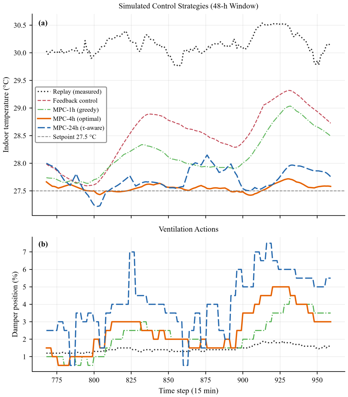
Table 12. Counterfactual control simulation (35-day record, setpoint 27.5 °C, $\lambda =0.02$) ^a.

Strategy	${\mathit{\sigma }}_{\mathit{T}}$ (K)	MAE from Setpoint (K)	Mean Damper (%)	Heater Fraction (0–1)	Energy (GJ)	Energy (kWh per bird per day)
Replay (measured actions)	4.26	3.82	4.48	0.40	4500	0.45
Proportional feedback	0.93	1.07	3.23	0.20	4080	0.41
MPC-1h	0.74	1.03	2.97	0.00	3702	0.37
MPC-4h ($\approx 0.7{\tau }_f$)	0.17	0.12	3.40	0.00	3711	0.37
MPC-8h ($\approx 1.5{\tau }_f$)	0.17	0.16	3.49	0.00	3711	0.37
MPC-24h	0.39	0.31	5.24	0.93	5431	0.55
MPC-48h	0.77	0.57	5.14	0.92	5428	0.54

^a Environment = calibrated lumped model (replay RMSE vs. measured = 2.53 K) driven by the measured outdoor-temperature record. MPC re-optimised hourly with a piecewise-constant sequence (1 h near piece + constant remainder; single piece at 1 h). Energy = ventilation heat removed + heater energy, the last column expressing it per bird per day for the 78,000 birds over the 35.5-day record. Only replay produced events outside 24–33 °C (326 above 33 °C and 765 below 24 °C); the proportional controller and all MPC variants held zero events. The optimum horizon is 4–8 h (≈$0.7$–1.5${\tau }_f$); longer horizons regulate looser and consume more energy (MPC-24h +47% vs. MPC-1h).

Table 12. Counterfactual control simulation (35-day record, setpoint 27.5 °C, $\lambda =0.02$) ^a.

Strategy	${\mathit{\sigma }}_{\mathit{T}}$ (K)	MAE from Setpoint (K)	Mean Damper (%)	Heater Fraction (0–1)	Energy (GJ)	Energy (kWh per bird per day)
Replay (measured actions)	4.26	3.82	4.48	0.40	4500	0.45
Proportional feedback	0.93	1.07	3.23	0.20	4080	0.41
MPC-1h	0.74	1.03	2.97	0.00	3702	0.37
MPC-4h ($\approx 0.7{\tau }_f$)	0.17	0.12	3.40	0.00	3711	0.37
MPC-8h ($\approx 1.5{\tau }_f$)	0.17	0.16	3.49	0.00	3711	0.37
MPC-24h	0.39	0.31	5.24	0.93	5431	0.55
MPC-48h	0.77	0.57	5.14	0.92	5428	0.54

^a Environment = calibrated lumped model (replay RMSE vs. measured = 2.53 K) driven by the measured outdoor-temperature record. MPC re-optimised hourly with a piecewise-constant sequence (1 h near piece + constant remainder; single piece at 1 h). Energy = ventilation heat removed + heater energy, the last column expressing it per bird per day for the 78,000 birds over the 35.5-day record. Only replay produced events outside 24–33 °C (326 above 33 °C and 765 below 24 °C); the proportional controller and all MPC variants held zero events. The optimum horizon is 4–8 h (≈$0.7$–1.5${\tau }_f$); longer horizons regulate looser and consume more energy (MPC-24h +47% vs. MPC-1h).

4. Discussion

The discussion follows the results in order: Section 4.1 unifies the single-step, multi-horizon and robustness results (Section 3.1 and Section 3.3) under the time constant, Section 4.2 attributes the two scales and the feature ranking (Section 3.2 and Section 3.5), Section 4.3 draws the control-design implications (Section 3.6), Section 4.4 the uncertainty lessons (Section 3.4), and Section 4.5 the limitations.

4.1. The $\tau$ Framework as a Unifying Explanation

Three seemingly independent results, the universal persistence floor at 15 min, the emergence of deep learning gains at horizons commensurate with $\tau$, and the horizon dependence of controller performance, are the same statement in three units. With $\tau =25.7$ h, a 15 min step resolves only 1.0% of the thermal response, so no model can extract information the current state does not already contain [20]. At 24 h (≈$1\tau$), the resolved fraction reaches 61%, enough for a nonlinear model to exploit the ventilation–temperature coupling [12,16,17] with stable, highly significant gains. The two scales split the control problem: the fast scale (${\tau }_f=5.5$ h) sets the preview needed for regulation (Section 3.6), while the slow scale governs the error growth that forecasting models must overcome; both scales are standard descriptors of the thermal response of buildings [43,44]. Within the limits of this single-house, single-winter case study, and of the uncertainty in $\tau$ itself (95% CI [10.5, 153.9] h; Section 3.2), the single parameter $\tau$ thus converts between model selection (Section 3.3), statistical significance (Section 3.3), and control design (Section 3.6) [22]. How accurately $\tau$ predicts model skill and control requirements in other house designs and climates remains to be tested.

4.2. Physical Origin of the Two Scales

The bi-exponential autocorrelation (${\tau }_f=5.5$ h, 8% of variance; ${\tau }_s\approx 189$ h, 92%) maps onto two physical heat stores: the chicken-plus-air mass ventilated through the house (fast), and the building fabric and floor (slow) [9,12,53]. This attribution is a physically motivated interpretation of the decomposition, not an independently validated result. Confirming the assignment of the two scales would require a step-response test or a validated building energy model. As quantified in Section 3.2, the slow scale is only partially identifiable within a 35-day record (the ACF decays just 22.4% over 48 h), so ${\tau }_s\approx 189$ h is an order-of-magnitude estimate, and its interpretation as a fabric-dominated store is provisional. The ventilation dependence of $\tau$ (56.6 to 21.7 h across the observed damper range) is the same mechanism: raising conductance shortens the fast store’s response. This dependence is predicted by the calibrated physical model; direct empirical estimation of $\tau \left(q\right)$ from the observational record was precluded by the lack of natural experiments in which damper position varies while other conditions remain fixed. Because the damper is itself the control actuator, and is the feature that dominates the 15 min residual in the SHAP analysis (Figure 8), the controller modulates predictability. This feedback loop between regulation and forecastability argues for joint design of sensing, prediction, and control, rather than optimizing the predictor in isolation.

These findings connect to, and partly reconcile, earlier livestock-house modelling results. In a year-round model of laying-hen houses, Liang et al. [12] reported that envelope thermal inertia induces only a small temperature delay (about 1 h in winter) and attenuation (1.02 K) when predicting the mean trajectory. The present decomposition shows why such small mean-level delays coexist with a dominant slow scale. The slow store (${\tau }_s\approx 189$ h) carries 92% of the variance of the fluctuation about the controlled mean, but it barely affects the mean trajectory itself, which the controller pins to the setpoint. Conversely, the failure of steady-state heat-balance models to track measured temperatures [7,8,9], also observed here (RMSE 3.7–13.1 K, Section 3.1), reflects the same physics: without the controller’s closed-loop action in the model, the slow store drives the simulated temperature away from the setpoint on a multi-day scale. Tunnel-ventilated winter studies [53] similarly show that the controller, not the envelope, sets the indoor thermal state. Quantitatively, the short-horizon floor found here (0.105 K at 15 min) and the multi-horizon errors (LSTM 0.455 K at 24 h; Table 5) fall within the 0.1–0.5 K range reported for livestock-house temperature models at 10–30 min horizons [12], which underlines that short-horizon accuracy, however high, does not by itself indicate model skill.

The two-scale picture also frames the role of spatial detail. CFD studies of broiler and layer houses report pronounced spatial temperature gradients, driven by inlet jets and tier geometry [23,24,25], as reproduced in microclimate simulations of commercial stocking [26]. More recent simulations extend this to coupled humidity and gas distributions [55], dynamic temperature variations [56], and three-dimensional temperature fields [57], as well as to lateral ventilation layouts [30] and cooling-season processes [58,59]. Vertical stratification at the bird level has been measured directly in the field [32,33,60]. These gradients matter for bird welfare and for sensor placement [35,38], and several studies have proposed their mitigation through inlet design [50,61], stratification control [62], and envelope measures [63]. The present analysis complements such spatial studies in the temporal domain: while CFD resolves where temperature differs, the time-constant framework explains when temperature can be expected to change, and it does so with a single scalar that is directly estimable from any sensor time series. The two perspectives can also be used together. The CFD results (or, more simply, the measured spatial spread of Section 2.1) identify the sensor locations that best represent the house mean, which matters because both the $\tau$ estimate and the forecast target are only as representative as the series they are computed from; the time constant estimated from those sensors then sets the horizons, with $\tau$_f fixing the preview of the controller (Section 4.3) and the lumped $\tau$ fixing the evaluation horizon of the forecaster (Section 4.1).

4.3. Practical Implications for Controller Design

Most commercial climate controllers recompute ventilation every 5–15 min from instantaneous temperature, implicitly assuming a short response. The simulation shows that once the controller can act on the heater as well as the dampers, a 1 h MPC horizon is already stable (zero band violations) but loose ($\sigma =0.74$ K), and that extending the horizon to 4–8 h (≈$0.7$–1.5${\tau }_f$) tightens regulation about fourfold ($\sigma =0.17$ K) at negligible extra energy. Horizons beyond ≈8 h are counterproductive: they regulate looser, consume more energy (MPC-24h +47% vs. MPC-1h), and are more sensitive to environment model error, because long rollouts accumulate the mismatch between the model and the executed environment. The 4–8 h optimum is not arbitrary: it is 1–1.5 times the fast scale ${\tau }_f$, the time scale on which the controller’s own actions actually move the indoor temperature. A corollary of the two-scale decomposition is that the preview horizon that matters for regulation is set by the fast scale, whereas the horizon at which learned forecasters pay off is set by the slow scale (Section 3.3); the two design questions should therefore not be conflated.

Two caveats bound these rules. First, read as a forecast-skill horizon, the reported lumped $\tau$ places the horizon at which learned models begin to pay off somewhere between about 10 h and 6 days for this house and season (95% CI [10.5, 153.9] h), so the value should be re-estimated rather than adopted. Second, the width of that interval is governed by the lag range rather than by the number of samples. The same six-horizon estimator applied to the full 35-day record gives a ±22% interval (5.8 h, 95% CI [4.8, 7.4] h) and has migrated towards the fast scale, while extending the horizons towards multi-day lags moves the estimate towards the slow scale (84 h at 8-day lags). Because the process is bi-exponential (Section 3.2), no single winter record pins a converged lumped $\tau$; a firm value would require multi-season records, whereas the control-relevant fast scale is tightly identified ([5.1, 5.9] h) and recoverable from a three-day record (Table 4).

These results support a suggested design rule: winter broiler-house controllers should use model-based preview of ≈$0.7$–1.5${\tau }_f$ (here 4–8 h), estimated from the ACF initial decay of a record of about three days (Section 3.2), with ${\tau }_f$ re-estimated for each house and season; regulators need not look as far ahead as one lumped $\tau$. They are also consistent with broader efforts to reduce poultry-house heating energy through passive measures and improved control [11,64,65].

4.4. Physical Priors vs. Data-Driven Uncertainty

The distribution-shift experiment (Section 3.4) carries a general lesson. Learned quantile regressors [52] are calibrated in-sample but fail out-of-sample when volatility changes, whereas the two-parameter theoretical band, a direct consequence of Equation (1), remains calibrated. This pattern echoes the general difficulty of constructing prediction intervals from learned models [46]. The interval score [45] makes the coverage–sharpness trade-off explicit: at horizons ≤ 4 h, the theoretical band scores better despite being wider, because the quantile band’s under-coverage penalty exceeds its sharpness gain. At 24 h, the quantile band wins on interval score but at 0.72 coverage, below the nominal 0.90. The appropriate choice therefore depends on the application: for operational risk metrics and controller constraints that require nominal coverage under shifting regimes, $\tau$-anchored intervals are preferable; if expected width is the sole criterion, learned bands can be sharper, but their coverage is not guaranteed when the regime shifts. Quantile methods should be recalibrated on recent data whenever the operating regime changes.

4.5. Limitations

Several caveats apply. The control simulation uses the calibrated analytical model as the environment; the environment itself carries the model’s 2.5 K replay error, so absolute trajectories are indicative rather than exact, and the relative ordering of strategies is the defensible output. The MPC used a piecewise-constant control sequence rather than a full control sequence, and the action-cost weight $\lambda$ is a free design parameter; the horizon ranking was, however, insensitive to refining the sequence and to a tenfold variation of $\lambda$ (Table 11), with only a tenfold larger action penalty, which degrades regulation at every horizon, shifting the optimum (Section 3.6). The heater was modelled with a binary hysteresis rule (on below 27 °C, off above 29 °C), which neglects heater thermal inertia and modulation; since all MPC strategies faced the same heater model, the ranking is unaffected, though absolute heating energy should be read with this simplification in mind.

Process-noise experiments showed that long-horizon MPC is more sensitive to model mismatch than short-horizon MPC: the recommended 4–8 h preview keeps a lower ${\sigma }_T$ than both the 1 h and the 24 h horizon under process noise, while the 1 h horizon preserves fewer violations at the strongest noise level (Table 10). The noise magnitudes tested (0.25–1.0 K) bracket a fraction of the environment’s 2.5 K replay error. The dataset covers one house, one winter, and one controller, whereas earlier field studies documented substantial variability across houses, ventilation modes, and seasons [32,34]. Note that $\tau$, its two scales, and the ventilation modulation should be re-estimated for other climates, house types, and stocking densities; the framework, not the specific numbers, is the transferable result. Attempts to classify imminent extreme events remained uninformative because no test window contained a positive event (Section 3.3); a multi-winter record would be required to assess short-horizon extreme-event prediction in this regime.

5. Conclusions

Seen as a control problem, a commercial broiler house in winter is a slow system with a fast actuator. Its thermal state carries the memory of roughly a day ($\tau$ = 25.7 h here), so at the 15 min resolution of the climate controller, the house has not yet responded to anything a model could exploit: every learned predictor matched persistence, and skill appeared only once a forecast spanned a meaningful fraction of that memory. The same two-scale structure decides the control side. The damper acts on the fast scale, so a preview of a few hours is enough; longer horizons accumulate model error without improving control in a house that changes on a slower clock.

The consequence is a division of labour between two design questions that are usually conflated. Forecasting models should be evaluated, and re-trained, on the scale of the house time constant, where their contribution becomes measurable; the control preview should be set on the scale of the ventilation response, a few hours, and re-estimated whenever ventilation practice or season shifts the balance, because the damper tunes the very time constant that governs predictability. Both scales are house- and season-specific, and so are the numbers; the framework—one lumped time constant, two scales, each matched to the question it answers—is expected to transfer to other mechanically ventilated livestock buildings.

References

- Deng, S.; Li, Z.; Wei, Y.; Wang, Y.; Li, B.; Zheng, W. Assessing temperature distribution inside commercial stacked cage broiler houses in winter. Animals 2024, 14, 2638. [Google Scholar] [CrossRef] [Scilit] [PubMed]
- Aviagen. Arbor Acres Broiler Management Handbook; Aviagen: Huntsville, AL, USA, 2022. [Google Scholar]
- Feddes, J.; Emmanuel, E.; Zuidhoft, M. Broiler performance, body weight variance, feed and water intake, and carcass quality at different stocking densities. Poult. Sci. 2002, 81, 774–779. [Google Scholar] [CrossRef] [Scilit] [PubMed]
- Xin, H.; Berry, I.L.; Tabler, G.T.; Barton, T.L. Temperature and humidity profiles of broiler houses with experimental conventional and tunnel ventilation systems. Appl. Eng. Agric. 1994, 10, 535–542. [Google Scholar] [CrossRef] [Scilit]
- Saeed, M.; Abbas, G.; Alagawany, M.; Kamboh, A.A.; Abd El-Hack, M.E.; Khafaga, A.F.; Chao, S. Heat stress management in poultry farms: A comprehensive overview. J. Therm. Biol. 2019, 84, 414–425. [Google Scholar] [CrossRef] [Scilit] [PubMed]
- Chen, S.; Yong, Y.; Ju, X. Effect of heat stress on growth and production performance of livestock and poultry: Mechanism to prevention. J. Therm. Biol. 2021, 99, 103019. [Google Scholar] [CrossRef] [Scilit] [PubMed]
- Cooper, K.; Parsons, D.; Demmers, T. A thermal balance model for livestock buildings for use in climate change studies. J. Agric. Eng. Res. 1998, 69, 43–52. [Google Scholar] [CrossRef] [Scilit]
- Schauberger, G.; Piringer, M.; Petz, E. Steady-state balance model to calculate the indoor climate of livestock buildings, demonstrated for finishing pigs. Int. J. Biometeorol. 2000, 43, 154–162. [Google Scholar] [CrossRef] [Scilit] [PubMed]
- Olgun, M.; Çelik, M.Y.; Polat, H.E. Determining of heat balance design criteria for laying hen houses under continental climate conditions. Build. Environ. 2007, 42, 355–365. [Google Scholar] [CrossRef] [Scilit]
- Wang, Y.; Li, B.; Liang, C.; Zheng, W. Dynamic simulation of thermal load and energy efficiency in poultry buildings in the cold zone of China. Comput. Electron. Agric. 2020, 168, 105127. [Google Scholar] [CrossRef] [Scilit]
- Kuczyński, T.; Staszczuk, A.; Gortych, M.; Stryjski, R. Effect of thermal mass, night ventilation and window shading on summer thermal comfort of buildings in a temperate climate. Build. Environ. 2021, 204, 108126. [Google Scholar] [CrossRef] [Scilit]
- Liang, C.; Yin, H.; Li, B.; Wang, C. Hourly model for predicting year-round temperature and relative humidity of the environment in laying hen houses. Trans. Chin. Soc. Agric. Eng. 2021, 37, 229–235. [Google Scholar] [CrossRef]
- Box, G.; Jenkins, G. Time Series Analysis: Forecasting and Control; Holden-Day: San Francisco, CA, USA, 1976. [Google Scholar]
- Chen, T.; Guestrin, C. XGBoost. In Proceedings of the 22nd ACM SIGKDD International Conference on Knowledge Discovery and Data Mining; ACM: New York, NY, USA, 2016; pp. 785–794. [Google Scholar] [CrossRef] [Scilit]
- Breiman, L. Random forests. Mach. Learn. 2001, 45, 5–32. [Google Scholar] [CrossRef] [Scilit]
- Hochreiter, S.; Schmidhuber, J. Long short-term memory. Neural Comput. 1997, 9, 1735–1780. [Google Scholar] [CrossRef] [Scilit] [PubMed]
- Vaswani, A.; Shazeer, N.; Parmar, N.; Uszkoreit, J.; Jones, L.; Gomez, A.; Kaiser, L.; Polosukhin, I. Attention is all you need. Proc. Adv. Neural Inf. Process. Syst. 2017, 30, 5998–6008. [Google Scholar]
- Lea, C.; Flynn, M.; Vidal, R.; Reiter, A.; Hager, G. Temporal convolutional networks for action segmentation and detection. In Proceedings of the 2017 IEEE Conference on Computer Vision and Pattern Recognition (CVPR); IEEE: Piscataway, NJ, USA, 2017; pp. 1003–1012. [Google Scholar] [CrossRef] [Scilit]
- Oreshkin, B.; Carpov, D.; Chapados, N.; Bengio, Y. N-BEATS: Neural basis expansion analysis for interpretable time series forecasting. In Proceedings of the International Conference on Learning Representations, New Orleans, LA, USA, 6–9 May 2019. [Google Scholar]
- Hyndman, R.; Athanasopoulos, G. Forecasting: Principles and Practice, 2nd ed.; OTexts: Melbourne, Australia, 2018; Available online: https://otexts.com/fpp2/ (accessed on 12 October 2026).
- Diebold, F.X.; Mariano, R.S. Comparing predictive accuracy. J. Bus. Econ. Stat. 1995, 13, 253–263. [Google Scholar] [CrossRef] [Scilit]
- Camacho, E.F.; Bordons, C. Model Predictive Control, 2nd ed.; Springer: London, UK, 2007. [Google Scholar] [CrossRef] [Scilit]
- Blanes-Vidal, V.; Guijarro, E.; Balasch, S.; Torres, A. Application of computational fluid dynamics to the prediction of airflow in a mechanically ventilated commercial poultry building. Biosyst. Eng. 2008, 100, 105–116. [Google Scholar] [CrossRef] [Scilit]
- Kwon, K.S.; Lee, I.B.; Zhang, G.Q.; Ha, T. Computational fluid dynamics analysis of the thermal distribution of animal occupied zones using the jet-drop-distance concept in a mechanically ventilated broiler house. Biosyst. Eng. 2015, 136, 51–68. [Google Scholar] [CrossRef] [Scilit]
- Cheng, Q.; Feng, H.; Meng, H.; Zhou, H. CFD study of the effect of inlet position and flap on the airflow and temperature in a laying hen house in summer. Biosyst. Eng. 2021, 203, 109–123. [Google Scholar] [CrossRef] [Scilit]
- Küçüktopcu, E.; Cemek, B.; Simsek, H.; Ni, J.Q. Computational fluid dynamics modeling of a broiler house microclimate in summer and winter. Animals 2022, 12, 867. [Google Scholar] [CrossRef] [Scilit] [PubMed]
- Küçüktopcu, E.; Cemek, B. Evaluating the influence of turbulence models used in computational fluid dynamics for the prediction of airflows inside poultry houses. Biosyst. Eng. 2019, 183, 1–12. [Google Scholar] [CrossRef] [Scilit]
- Rong, L.; Nielsen, P.V.; Bjerg, B.; Zhang, G. Summary of best guidelines and validation of CFD modeling in livestock buildings to ensure prediction quality. Comput. Electron. Agric. 2016, 121, 180–190. [Google Scholar] [CrossRef] [Scilit]
- Norton, T.; Grant, J.; Fallon, R.; Sun, D.W. Assessing the ventilation effectiveness of naturally ventilated livestock buildings under wind dominated conditions using computational fluid dynamics. Biosyst. Eng. 2009, 103, 78–99. [Google Scholar] [CrossRef] [Scilit]
- Trokhaniak, V. Investigation of the lateral ventilation system in a poultry house using CFD. Nauk. Žurnal Teh. Energ. 2022, 13, 81–91. [Google Scholar] [CrossRef] [Scilit]
- Ameen, A.; Yamasawa, H.; Kobayashi, T. Numerical evaluation of the flow field of an isothermal dual-corner impinging jet for building ventilation. Buildings 2022, 12, 1767. [Google Scholar] [CrossRef] [Scilit]
- Wheeler, E.; Zajaczkowski, J.; Weiss, R.; Hulet, R. Temperature stratification and fuel use during winter in three Pennsylvania broiler houses. J. Appl. Poult. Res. 2000, 9, 551–563. [Google Scholar] [CrossRef] [Scilit][Green Version]
- Boshouwers, F.M.G.; Davelaar, F.G.; Landman, W.J.M.; Nicaise, E.; Van den Bos, J. Vertical temperature profiles at bird level in broiler houses. Br. Poult. Sci. 1996, 37, 55–62. [Google Scholar] [CrossRef] [Scilit] [PubMed]
- Wheeler, E.F.; Zajaczkowski, J.L.; Sabeh, N.C. Field evaluation of temperature and velocity uniformity in tunnel and conventional ventilation broiler houses. Appl. Eng. Agric. 2003, 19, 321–330. [Google Scholar] [CrossRef] [Scilit]
- Jia, Y.; Li, L.; Gao, L. Research on virtual collection method of layer house temperature for the construction requirements of digital twin system. Poult. Sci. 2025, 104, 104771. [Google Scholar] [CrossRef] [Scilit] [PubMed]
- Zheng, W.; Xiong, Y.; Gates, R.; Wang, Y.; Koelkebeck, K. Air temperature, carbon dioxide, and ammonia assessment inside a commercial cage layer barn with manure-drying tunnels. Poult. Sci. 2020, 99, 3885–3896. [Google Scholar] [CrossRef] [Scilit] [PubMed]
- Wen, P.; Li, L.; Xue, H.; Jia, Y.; Gao, L.; Li, R.; Huo, L. Comprehensive evaluation method of the poultry house indoor environment based on gray relation analysis and analytic hierarchy process. Poult. Sci. 2022, 101, 101587. [Google Scholar] [CrossRef] [Scilit] [PubMed]
- Çaylı, A. Assessment on spatial variability of temperature and relative humidity in a tunnel ventilated broiler house. J. Anim. Plant Sci. 2025, 35, 739–746. [Google Scholar] [CrossRef] [Scilit]
- Pedersen, S.; Takai, H.; Johnsen, J.; Metz, J.; Groot Koerkamp, P.; Uenk, G.; Phillips, V.; Holden, M.; Sneath, R.; Short, J.; et al. A comparison of three balance methods for calculating ventilation rates in livestock buildings. J. Agric. Eng. Res. 1998, 70, 25–37. [Google Scholar] [CrossRef] [Scilit]
- Larsen, T.S.; Heiselberg, P. Single-sided natural ventilation driven by wind pressure and temperature difference. Energy Build. 2008, 40, 1031–1040. [Google Scholar] [CrossRef] [Scilit]
- Yi, Q.; Wang, X.; Zhang, G.; Li, H.; Janke, D.; Amon, T. Assessing effects of wind speed and wind direction on discharge coefficient of sidewall opening in a dairy building model—A numerical study. Comput. Electron. Agric. 2019, 162, 235–245. [Google Scholar] [CrossRef] [Scilit]
- Elghardouf, N.; Lahlouh, I.; Elakkary, A.; Sefiani, N. Towards modelling, and analysis of differential pressure and air velocity in a mechanical ventilation poultry house: Application for hot climates. Heliyon 2023, 9, e12936. [Google Scholar] [CrossRef] [Scilit] [PubMed]
- Hagentoft, C.E. Introduction to Building Physics; Studentlitteratur: Lund, Sweden, 2001. [Google Scholar]
- CIBSE. Guide A: Environmental Design, 7th ed.; The Chartered Institution of Building Services Engineers: London, UK, 2006. [Google Scholar]
- Gneiting, T.; Raftery, A.E. Strictly proper scoring rules, prediction, and estimation. J. Am. Stat. Assoc. 2007, 102, 359–378. [Google Scholar] [CrossRef] [Scilit]
- Khosravi, A.; Nahavandi, S.; Creighton, D.; Atiya, A.F. Comprehensive review of neural network-based prediction intervals and new advances. IEEE Trans. Neural Netw. 2011, 22, 1341–1356. [Google Scholar] [CrossRef] [Scilit] [PubMed]
- ASHRAE. Handbook of Fundamentals; Technical report; American Society of Heating, Refrigerating and Air-Conditioning Engineers: Atlanta, GA, USA, 2017. [Google Scholar]
- Albright, L. Environment Control for Animals and Plants; American Society of Agricultural Engineers: St. Joseph, MI, USA, 1990. [Google Scholar]
- Manshor, N.; Abdul Rahiman, A.R.; Yazed, M.K. IoT based poultry house monitoring. In Proceedings of the 2019 2nd International Conference on Communication Engineering and Technology (ICCET); IEEE: Piscataway, NJ, USA, 2019; pp. 72–75. [Google Scholar] [CrossRef] [Scilit]
- Hoff, S.J.; Wu, C.G. Establishing criteria for sidewall air inlet performance and evaluation of four commercial inlets on this criteria. Trans. ASAE 2000, 43, 735–743. [Google Scholar] [CrossRef] [Scilit][Green Version]
- Calvet, S.; Estellés, F.; Cambra-López, M.; Torres, A.G.; Van den Weghe, H.F.A. The influence of broiler activity, growth rate, and litter on carbon dioxide balances for the determination of ventilation flow rates in broiler production. Poult. Sci. 2011, 90, 2449–2458. [Google Scholar] [CrossRef] [Scilit] [PubMed]
- Koenker, R.; Bassett, G. Regression quantiles. Econometrica 1978, 46, 33–50. [Google Scholar] [CrossRef] [Scilit]
- Ma, H.; Tu, Y.; Yang, X.; Yang, Z.; Liang, C. Influence of tunnel ventilation on the indoor thermal environment of a poultry building in winter. Build. Environ. 2022, 223, 109448. [Google Scholar] [CrossRef] [Scilit]
- Lundberg, S.; Lee, S.I. A unified approach to interpreting model predictions. Proc. Adv. Neural Inf. Process. Syst. 2017, 30, 4765–4774. [Google Scholar]
- Ahmadi Babadi, K.; Khorasanizadeh, H.; Aghaei, A. CFD modeling of air flow, humidity, CO2 and NH3 distributions in a caged laying hen house with tunnel ventilation system. Comput. Electron. Agric. 2022, 193, 106677. [Google Scholar] [CrossRef] [Scilit]
- Choi, L.Y.; Daniel, K.F.; Lee, S.Y.; Lee, C.R.; Park, J.Y.; Park, J.; Hong, S.W. CFD simulation of dynamic temperature variations induced by tunnel ventilation in a broiler house. Animals 2024, 14, 3019. [Google Scholar] [CrossRef] [Scilit] [PubMed]
- Ferraz, P.F.P.; Andrade, E.T.D.; Vilas Boas, R.B.; Rezende, R.P.; Yanagi Junior, T.; Barbari, M. Three-dimensional simulation of the temperature distribution in a commercial broiler house. Animals 2022, 12, 1278. [Google Scholar] [CrossRef] [Scilit] [PubMed]
- Hu, C.; Li, L.; Jia, Y.; Xie, Z.; Yu, Y.; Huo, L. Numerical study and optimization of thermal environment regulation in poultry house ventilation systems. Poult. Sci. 2025, 104, 105786. [Google Scholar] [CrossRef] [Scilit] [PubMed]
- Trokhaniak, V.; Synyavskiy, O.; Tkachuk, V.; Lillerand, T.; Skliar, O.; Ihnatiev, Y.; Olt, J. Numerical simulation of air cooling processes in a poultry house with a tunnel-side ventilation system. INMATEH Agric. Eng. 2025, 75, 640–647. [Google Scholar] [CrossRef] [Scilit]
- Miles, D. Vertical stratification of ammonia in a broiler house. J. Appl. Poult. Res. 2008, 17, 348–353. [Google Scholar] [CrossRef] [Scilit]
- Peng, H.; Li, B.; Chen, C.; Deng, S.; Zheng, W.; Wang, Y. Effects of sidewall inlet parameters on the airflow and temperature field in poultry houses with an alternative ventilation system. J. ASABE 2025, 68, 37–50. [Google Scholar] [CrossRef] [Scilit]
- Shah, S.B.; Earnest, K.; Oviedo-Rondón, E.O.; Kolar, P.; Singletary, I. Simultaneous reduction of thermal stratification and ammonia concentrations in poultry house during brooding and in cool weather. Appl. Eng. Agric. 2022, 38, 375–386. [Google Scholar] [CrossRef] [Scilit]
- Wang, Y.; Zheng, W.; Shi, H.; Li, B. Optimising the design of confined laying hen house insulation requirements in cold climates without using supplementary heat. Biosyst. Eng. 2018, 174, 282–294. [Google Scholar] [CrossRef] [Scilit]
- Elsaid, M.A.; Kishk, S.; ElMasry, G.; ElGamal, R. Performance evaluation of a solar heating system for poultry house. J. Anim. Poult. Fish. Prod. 2025, 14, 32–47. [Google Scholar] [CrossRef] [Scilit]
- Jalali, M.; Banakar, A.; Farzaneh, B.; Montazeri, M. Reducing energy consumption in a poultry farm by designing and optimizing the solar heating/photovoltaic system. Sustainability 2023, 15, 6059. [Google Scholar] [CrossRef] [Scilit]
Disclaimer/Publisher’s Note: The statements, opinions and data contained in all publications are solely those of the individual author(s) and contributor(s) and not of MDPI and/or the editor(s). MDPI and/or the editor(s) disclaim responsibility for any injury to people or property resulting from any ideas, methods, instructions or products referred to in the content. |
© 2026 by the authors. Licensee MDPI, Basel, Switzerland. This article is an open access article distributed under the terms and conditions of the Creative Commons Attribution (CC BY) license.