


Abstract
As cities densify, urban green infrastructure and artistic landscaping, the deliberate arrangement of plants into visual compositions, carry ecological and public-health weight, yet manual execution does not scale. This article presents ARTgriculture 2.0, a redesigned Internet-of-Things-enabled unmanned ground vehicle that automates the full seeding cycle of digging, sowing, backfilling, and spraying for artistic landscaping, extending our earlier conference prototype. The platform introduces iris-seeding, variable-gap, and depth-control mechanisms sized and fabricated for compositional planting, a layered control architecture, and a browser-based interface for autonomous and manual operation. The redesigned mechanisms were fabricated and exercised on the physical chassis in indoor bench tests, without soil engagement and with no seed lot loaded, and no field trial has been performed; the validation level reported here is therefore module-level bench actuation plus system-level simulation. Full-system seeding is evaluated with a simulation model: a robot model built in NVIDIA Isaac Sim supplies the geometry and scene, while an offline kinematic execution model plans and executes area-fill coverage over regular grids and artistic patterns such as circles, diamonds, and hearts. Under the undisturbed model at a conservative low cruise speed, the platform reaches 96 to 100 percent seed placement at 2.4 to 3.4 cm mean tracking error and completes 15 m scale fields in 13 to 21 min; these are model values, not measurements. A Monte Carlo study of 30 runs per pattern that adds odometry noise, actuation-lag variation, wheel slip, lateral drift, and initial pose error holds mean coverage within 2.0 percentage points of the undisturbed values but roughly doubles mean tracking error, to 5.2 to 6.1 cm, and tightening the placement tolerance from 0.45 m to 0.15 m lowers coverage to 86.0 to 92.3 percent on the same trajectories, 90.1 to 92.3 percent in the reduced-speed mode. The functional prototype cost roughly 600 to 700 USD to build. The results indicate that pattern-precise, low-cost robotic seeding is achievable in simulation and identify soil-engaged field testing and quantified seed metering as the decisive next steps.
1. Introduction
Urbanization is reshaping the planet’s surface at an unprecedented pace, and more than two-thirds of the global population is projected to live in cities by 2050 [1]. This concentration of people intensifies pressure on urban ecosystems and turns the deliberate cultivation of green space into a matter of public health rather than decoration. Robotics and autonomous systems are increasingly seen as instruments that will shape those ecosystems, from irrigation and monitoring to planting, yet their net effect on urban green space remains an open question that depends heavily on how the technology is designed and deployed [2].
Within urban greening, artistic landscaping, the deliberate spatial arrangement of plant species into visual compositions, delivers ecological and cultural value at once [3,4]. Its adoption is constrained less by horticultural knowledge than by execution. Intricate planting patterns demand time-intensive planning, skilled labour, and context-sensitive placement, which limits their scalability in fast-growing cities. Recent work has begun to bring automation to urban vegetation, including robot-inclusive vertical greenery [5], compact urban farming robots [6], and autonomous mowers whose movement patterns already influence garden design [7]. These efforts show the promise of automation, but none targets the pattern-precise, multi-task seeding that artistic landscaping requires.
Over the past decade, agricultural robotics has matured into a broad field, and unmanned ground vehicles (UGVs) now perform seeding, weeding, spraying, and monitoring across many crops [8,9,10]. Recent reviews document rapid progress in platforms, sensing, and autonomy for precision agriculture [11,12]. This body of work supplies the building blocks for an urban landscaping robot, but it is optimized for large, uniform fields rather than the spatial precision and creative intent of artistic planting.
Three capabilities are central to bridging that gap, and each has a substantial literature. First, seed placement depends on the metering mechanism, with studies ranging from dedicated seed-planting UGVs [13] to metering devices validated by discrete element simulation [14] and closed-loop metering under fuzzy PID control [15,16]. Second, field productivity depends on coverage path planning, the problem of visiting every target while minimizing travel and turns; the topic is well surveyed [17,18], with open-source libraries [19] and complete-coverage methods for wheeled robots [20,21]. Third, autonomy rests on navigation and mapping, where Robot Operating System (ROS) stacks with LiDAR SLAM and probabilistic localization are now standard [22,23,24]. Layered over all three, the Internet of Things (IoT) provides the remote sensing, control, and monitoring that make such systems usable at scale [25,26,27]. Increasingly, these capabilities are first evaluated in simulation, and ROS, Gazebo, and Isaac Sim simulation models of agricultural robots have become a standard step before field trials [28,29].
Despite this progress, a clear gap remains. The literature concentrates on productivity in monoculture fields, while robotic support for urban and artistic landscaping is nascent and fragmented [2,5,6,7]. The individual capabilities are each well established, and several of the systems reviewed below deliver one or two of them well; what we did not find in the published literature is their combination on a single low-cost platform, namely a full dig, sow, backfill, and spray cycle together with area-fill coverage of arbitrary artistic polygons and an install-free IoT control layer, evaluated in a reproducible way. Table 1 sets out how the closest published systems compare on placement accuracy, speed, autonomy, coverage capability, and cost, and makes the basis of that claim explicit rather than asserting it.
Table 1.
Comparison of representative seeding and planting systems. An em-dash means the quantity is not reported in the cited source; no value in this table is estimated.
This article addresses that gap with ARTgriculture 2.0, a redesigned second-generation platform that extends our earlier conference contribution [30]. Because a conference extension must be explicit about what is new, the technical delta is stated item by item. (i) Seeding mechanism: the fixed-disk seed metre of the conference prototype is replaced by an iris mechanism whose aperture is continuously adjustable to 26 mm, so a seed class is selected by software command instead of by swapping a disk. (ii) Cultivator: the fixed cultivator is replaced by a variable-gap dual-arm linkage in which one NEMA 34 stepper opens and closes both arms symmetrically, and the rear land-levelling mechanism repeats the same linkage. (iii) Low-level controller: the STM32F401 is replaced by an Arduino Mega 2560 for its larger input and output count, with the ESP8266 command protocol unchanged so the operator interface drives either controller. (iv) Navigation and perception: the conference paper described no navigation or perception stack; this article adds a Raspberry Pi 4 running a ROS navigation stack with a Kinect v1 depth sensor and an MPU-6050 inertial unit. (v) Coverage planning: the conference grid rule for rectangles is generalized to an area-fill scanline planner that clips boustrophedon rows to an arbitrary polygon. (vi) Quantified performance: the conference paper reported component specifications and design parameters but no accuracy, coverage, drive-control, or cost figures; this article is the first to report per-pattern coverage and tracking metrics for five shape families, an identified drive plant with closed-loop step-response metrics, a Monte Carlo disturbance analysis of the execution model, and an itemized build cost. The digging depth law and the three timed spray dose levels are carried over unchanged and are reported here as continuity, not as novelty. Because further physical experiments were not feasible, the integrated platform is evaluated with a simulation model rather than in the field, an approach that is standard practice before field trials [28,29].
The contributions of this work are as follows.
- A redesigned ARTgriculture 2.0 platform with iris-seeding, variable-gap, and depth-control mechanisms, presented with its design methodology, structural analysis, and motor sizing.
- Area-fill coverage path planning that generalizes boustrophedon rows from rectangles to arbitrary artistic polygons, executed in an offline kinematic simulation model and compared against a bounding-box boustrophedon baseline.
- An IoT web and application layer for autonomous and manual operation, monitoring, and progress tracking.
- A simulation study that evaluates area-fill seeding coverage over regular grids and artistic patterns, extended with a Monte Carlo disturbance analysis and a placement-tolerance sensitivity analysis, together with a cost analysis of the roughly 600 to 700 USD prototype.
The remainder of the paper is organized as follows. Section 2 reviews related work. Section 3 presents the system overview. Section 4, Section 5 and Section 6 detail the mechanical, electronic, and control design. Section 7 covers autonomous navigation, coverage path planning, and the simulation model used to execute the plans, including the disturbance model added in this revision. Section 8 describes the IoT interface. Section 9 reports results and validation. Section 10, Section 11 and Section 12 cover cost, discussion, and conclusions.
2. Related Work
2.1. Agricultural UGVs and Multi-Task Robots
Unmanned ground vehicles have become a workhorse of precision agriculture. Overviews describe platforms that seed, spray, and monitor autonomously [10], while dedicated systems target continuous crop monitoring [8] and general field operations [9]. Broad reviews map the design space of platforms, sensors, and evaluation methods [11,12]. These systems establish the mechanical and autonomy building blocks reused here, but they are tuned for large, uniform fields, which leaves the pattern precision and site variability of urban artistic landscaping unaddressed. Recent field evaluations of autonomous ground robots for real farming operations report practical constraints on speed, autonomy, and energy use that motivate careful drive-level characterization [31].
2.2. Seeding and Planting Mechanisms
Accurate seed placement is a mature subfield. Owoeye et al. [13] built a UGV dedicated to seed planting with an integrated selector and metering unit. Metering-device research emphasizes singulation accuracy, from discrete-element design of high-speed metering disks [14] to motor-driven metering with fuzzy PID control [16], and reviews summarize the mechatronics of precision sowing [15]. This work adapts the same precision goals but replaces row-crop metering with an iris-seeding mechanism and a variable-gap layout suited to compositional, rather than row, planting.
2.3. Coverage Path Planning
Coverage path planning (CPP) determines how a robot visits an entire work area efficiently. Short and comprehensive reviews frame the problem for agricultural ground robots [17,18], open-source tooling such as Fields2Cover has standardized common routines [19], and complete-coverage methods address wheeled robots and curvature constraints [20,21]. Existing methods overwhelmingly assume rectangular fields covered by boustrophedon passes. Artistic layouts, where target points fill a shape rather than a grid, are not addressed, which motivates the area-fill coverage developed in Section 7.
2.4. Autonomous Navigation and Mapping
Field autonomy is now commonly built on ROS with LiDAR SLAM and probabilistic localization. Reported systems span greenhouse robots fusing 2D and 3D LiDAR [23], field-inspection robots combining map construction with positioning [24], and autonomous exploration and navigation stacks built directly on ROS [22]. Our platform follows this established stack, using SLAM for mapping, adaptive Monte Carlo localization, and a standard planner, with the Kinect v1 depth sensor rather than a dedicated LiDAR unit supplying the scan data (Section 5); the planar motion of that layer is what the simulation model reproduces.
2.5. IoT and Simulation for Agricultural Robots
The Internet of Things underpins remote operation, sensing, and control in modern agriculture, as documented in comprehensive surveys [25,26,27]. In parallel, simulation has become the standard proving ground before field deployment, with ROS, Gazebo, and Isaac Sim simulation models used to develop and test agricultural robots and their navigation [28,29]. This work joins the two threads, pairing an IoT web and application control layer with a simulation-first evaluation strategy. Simulation is used here as a substitute for field trials that were not feasible, not as a substitute for field validation: it makes the reported results reproducible, and it bounds the model’s sensitivity to plausible disturbances, but it cannot establish agreement with hardware.
2.6. Comparative Positioning
Table 1 places ARTgriculture 2.0 against the seeding and planting systems it draws on. Field-tested metering mechanisms report qualified-placement rates from about 93 percent to above 98 percent under row-crop conditions [14,16], and a comparable UGV seed planter reports 94 percent field seed-delivery accuracy against a lower 66.67 percent metering-specific figure [13]. Reported forward speeds range from 0.71 to 0.77 m/s for a field robot under towed load [31] to 1.4 to 3.3 m/s for high-speed metering trials [14]. ARTgriculture 2.0 has not been measured against any of these physical benchmarks: its 95.6 to 100 percent figure is a simulated target-visitation rate produced by an offline kinematic execution model, not a physical seed-deposition accuracy, and no metering test of the iris mechanism has been run with seed. What the platform offers that none of the comparators do is the combination of low-cost construction, an arbitrary-polygon area-fill planner rather than row-only coverage, and a full dig, sow, backfill, and spray cycle. The honest claim is pattern-capable and simulation-evaluated, not field-validated.
3. ARTgriculture 2.0 System Overview
ARTgriculture 2.0 is a redesign of the conference prototype [30], built on the same chassis concept: a four-wheel-drive platform that digs, sows, backfills, and sprays in a single pass. The redesign replaces the fixed cultivator with a variable-gap dual-arm mechanism and the fixed-disk seed metre with an iris mechanism, and adds a rear spraying module and tool interchangeability at both ends of the chassis. The system is organized in four layers. The mechanical layer (Section 4) carries the seeding mechanisms. The electronics layer (Section 5) couples a Raspberry Pi 4 for navigation, an Arduino Mega 2560 for mechanism control, and an ESP8266 for wireless communication. The control layer (Section 6) covers seven subsystems: closed-loop control of the variable-gap position and the drive-wheel velocity, timed open-loop actuation of depth, iris metering, and spraying, and continuous polling of the environmental sensors and the GPS module. The IoT layer (Section 8) exposes autonomous and manual operation in a browser. Two scope statements belong here because they bound everything that follows. First, the platform sows one seed lot per run: the two tanks hold a single species at a time, and multi-species composition within one run is not supported. Second, ARTgriculture 2.0 was physically built. The redesigned mechanisms, the iris seeder, the variable-gap dual-arm linkage, and the depth-control unit, were fabricated and bench-tested on the platform chassis in July 2024, and the recordings provided as Supplementary Videos S1–S7 are of those fabricated 2.0 modules on that chassis, not of the earlier conference prototype. Figure 1 labels the subsystems on the CAD model, Figure 2 shows the fabricated prototype, and Table 2 summarizes the specification.
Figure 1.
The ARTgriculture 2.0 platform and its subsystems (chassis, seed tanks, sprayer, cultivator arms, land-levelling mechanism, wheel brackets).
Figure 2.
The fabricated ARTgriculture 2.0 prototype.
Table 2.
ARTgriculture 2.0 specification.
4. Mechanical Design
4.1. Design Methodology
Five constraints fixed the design space: modularity, so that tools such as sprayers, diggers, or seed units can be added or exchanged; cost-effective production; domestic manufacturability; suitability for off-road field conditions, including protection of the electronics; and novelty over the first prototype. Within these constraints, every mechanism passed through the same seven-step procedure: clarify the purpose and its limits, generate concepts by sketching, analyze the nature of loading, select the material, size the parts by force and stress analysis with failure theories, adjust shape for manufacturability and assembly (DFM and DFA), and produce working drawings with dimensions, tolerances, and finishes.
Concept selection followed two rules: keep the element count minimal and integrate form, feature, and function. Candidate concepts for each subsystem, among them hydraulic multi-tool rows, retractable V-shaped arms, multi-chamber seed tanks, and oscillating sprayers, were screened against the constraints; the selected set is the variable-gap dual-arm cultivator, the iris seed metre, the twin-tank sprayer, and interchangeable tool mounts. Loading on the structural members is static and essentially constant, so parts were sized against yield with a static factor of safety. Load-bearing links and frames are steel, cut from 1 mm sheet and 20 by 20 mm square tube, while the iris mechanism is 3D-printed plastic, which suffices because it carries only seed weight.
4.2. Structural Analysis and Motor Sizing
Six load-bearing components were analyzed in SolidWorks Simulation 2023 (Dassault Systèmes SolidWorks Corporation, Waltham, MA, USA) as linear static studies using von Mises stress and resultant-displacement plots (Figure 3): the grooved, centre, and slotted links of the variable-gap linkage, the seed-tank holder, and the nozzle holder and its base mount. Loading on these members is static and essentially constant, so each part was screened against the yield strength of its assigned material with a stress-based factor of safety. Table 3 reports the maximum von Mises stress, the maximum resultant displacement, and the resulting factor of safety for each study.
Figure 3.
Static finite-element studies of representative load-bearing components: (a) seed-tank holder, von Mises stress, fixed at the chassis-side end (left) with the tank load applied along the upper edges, maximum 408.7 MPa at the fixed end against a 460 MPa yield strength; (b) seed-tank holder, resultant displacement, maximum 15.3 mm at the free end; (c) grooved link, von Mises stress, maximum 10.32 MPa; (d) nozzle holder, von Mises stress, maximum 0.071 MPa. Colour scales are as reported by the CAD environment. Green arrows mark the fixed supports and red arrows mark the applied loads. The colour-bar values are shown in the E notation exported by the software, e.g., 4.087E+08 denotes 4.087 × 10⁸ Pa.
Table 3.
Static structural analysis results for the analyzed load-bearing components. Factors of safety are stress-based, computed as the displayed material yield strength divided by the maximum von Mises stress.
The seed-tank holder is the governing case and is reported here explicitly rather than folded into a blanket statement. It reaches a maximum von Mises stress of 408.7 MPa against the 460 MPa yield strength used in the study, so its stress-based factor of safety is FoS = σy/σmax = 460/408.7 ≈ 1.13, and its maximum resultant displacement is 15.3 mm, two to three orders of magnitude larger than any other analyzed part. These two numbers describe one mechanical situation and should be read together. The holder is a thin-walled sheet-steel part, formed from the 1 mm sheet specified in Section 4.1, that supports the seed tank from the chassis: an open rectangular frame of four sheet walls, fixed at its chassis-side end and loaded along its upper edges by the tank weight, so that it acts as a cantilever (Figure 3a,b). The peak stress occurs at the fixed end and the maximum displacement at the free end, as the plots show. For a thin plate or bracket loaded in bending, the peak bending stress scales with 1/t2 and the elastic deflection with 1/t3, where t is the sheet thickness, so a 1 mm section produces both a high local stress at the bend and a large elastic deflection under a moderate load. The 15.3 mm is the elastic displacement predicted by the linear static study, not permanent deformation: the peak stress stays below the yield value, so the model reports no yielding. The margin is nevertheless thin. An overload of 13 percent above the modelled case, or a yield strength 13 percent below the generic library value, would take the bend into yield, and a 15 mm deflection is a functional defect on its own because it would displace the tank outlet relative to the iris disk mounted beneath it. For both reasons the holder is identified as the first item for structural redesign. Doubling the sheet thickness to 2 mm with the geometry and load unchanged would, by the scaling above, reduce the peak bending stress by about a factor of four and the deflection by about a factor of eight; a gusseted or folded box section would give a comparable gain with less added mass. That margin is adequate against yield for a static screening but leaves no allowance for dynamic loading, fatigue, or manufacturing scatter.
Three limitations of these studies should be read alongside the numbers. The material assigned to each steel part is the generic library material of the CAD environment, displayed with a yield strength of 460 MPa; the specific steel grade, its Young’s modulus, and its supply condition are not recorded in the project’s design documentation, so the factors of safety in Table 3 are relative to that displayed value rather than to a certified material property. The applied-load magnitudes and the fixed and loaded faces were set in the CAD environment but were not archived numerically, so the load cases cannot be restated here in newtons; only the resulting stress and displacement fields were retained. Finally, the two intermediate links of the five-link chain were never analyzed. Table 3 is therefore reported as the design-stage screening it was, not as a verified structural qualification, and a documented structural study with stated load cases is listed as future work.
Motor sizing started from the variable-gap mechanism, the most heavily loaded actuator. With the arm weight and the drag of dry sand acting at an 85 mm lever, the required force is 76.2 N, so the torque demand is 76.2 N × 0.085 m, about 6.48 N.m. A NEMA 34 stepper with roughly 7 N.m holding torque covers this with margin, and an electromagnetic brake holds the position without keeping the coils energized. The drive train uses four 24 V, 48 W DC gear motors that deliver 9 N.m at 40 r/min through a 65.5:1 reduction. The electrical design was sized from a worst case in which every subsystem draws its rated power continuously. Summing the rated powers of Table 4 gives 499 W: 192 W for the four drive motors, 144 W for the NEMA 17 steppers, 80 W and 40 W for the NEMA 34 and NEMA 23, 20 W for the linear motors, 12 W for the pumps, and 11 W for the GPS module and the power electronics. Held for four hours this is 1996 Wh, close to 2.0 kWh, which is the figure the platform was sized against.
Table 4.
Power budget. Worst-case columns are the platform’s own rated-power sizing basis; duty-cycle columns are an illustrative scenario in which every duty-cycle value is an assumption, not a measurement.
Energy is supplied by 24 V lithium-ion packs assembled from 18,650 cells in a 6S3P arrangement behind 6S battery-management boards, with XL4015 buck converters supplying the control electronics and logic rails; the build records list 48 cells and two battery-management boards. The per-cell capacity rating was not recorded in the project’s bill of materials, so the total stored energy of the installed packs cannot be stated, and the 24 V, 100 Ah battery listed in the first-generation specification [30] was not carried over to this build. The demand side is therefore reported in full instead: the worst-case draw of Table 4 sums to 499 W, or 1996 Wh over a four-hour mission with every subsystem continuously active, and the duty-weighted column shows how strongly intermittent operation reduces the average load. The 3 to 4 h endurance figure inherited from the first-generation specification is reported in Table 2 as a design target rather than a measured or computed result: no endurance run has been performed on the 2.0 platform, and verifying the target requires recording the installed cell capacity and a discharge test, which we list as future work.
Because the mechanisms in fact operate sequentially within the seeding cycle, the average draw is far below the worst case. The right-hand columns of Table 4 show what that means arithmetically under one illustrative duty-cycle scenario. Every duty-cycle figure in those columns is an assumption, chosen to show the shape of the calculation; none is measured, and no mission-profile logging exists for the physical platform. Under those assumptions the average draw is about 122 W, which the main battery would sustain for roughly 19.7 h. That number is not claimed as an endurance figure. It is shown only to make clear that the gap between the 2.0 kWh worst-case sum and the 3 to 4 h target is a duty-cycle effect, and that resolving it properly requires mission-profile measurement on the physical platform, which is listed as future work.
4.3. Sowing and Variable-Gap Mechanism
The sowing subsystem couples two seed tanks to a dual-arm cultivator whose inter-arm gap is adjustable. A five-link chain—a centre link, two intermediate links, two slotted links, and two grooved links—is driven at its centre by the NEMA 34 stepper, so a single motor symmetrically opens or closes both cultivator arms to match the inter-row spacing of the crop or pattern (Figure 4). Each seed tank sits directly above one arm, so the seed drop follows the arm gap without a separate adjustment, and the land-levelling mechanism at the rear repeats the same linkage so that levelling stays aligned with the cultivated rows. A rotatable base under each tank sets the intra-row spacing between consecutive seeds.
Figure 4.
Sowing mechanism with the variable-gap linkage and seed tanks.
4.4. Iris Seeding Mechanism
The iris mechanism addresses a practical limitation of small seeders: conventional metering disks are machined for one seed size, so changing crop means changing disks. Borrowing the shutter principle of a camera aperture, six overlapping blades form an opening that is continuously adjustable from fully closed to 26 mm, wide enough for seeds up to roughly the thickness of an avocado seed, with a computed blade width of about 13.6 mm (Figure 5). One stepper motor rotates the blade ring to set the aperture for the selected seed class, and a second stepper drives a seed-flow fan under the tank that singulates seeds toward the opening. The fabricated seed disk is shown in Figure 6. The same hardware therefore metres small grains and large seeds with a software command instead of a mechanical swap.
Figure 5.
Iris seeding mechanism, gear and servo drive of the iris blades.
Figure 6.
The fabricated iris seed disk.
The design basis for the three seed classes follows directly from that geometry. The aperture opens continuously from fully closed to 26 mm, which spans the size range from small grains to a seed roughly the thickness of an avocado seed, and each class command sets both the aperture and the number of seeds released per hole, five for small, three for medium, and one for large (Section 6.3). The aperture is sized to pass the largest seed of its class without bridging while remaining small enough that the class below cannot pass more than its commanded count in one blade cycle. This is a design rationale, not a measurement: the mechanism has not been operated with a seed lot, so no singulation rate, missed-seed rate, or double-seed rate exists for it, and none is claimed anywhere in this article. A bench metering trial across the three size classes is the first physical test identified in Section 12.
4.5. Spraying Mechanism
The spraying module carries two detachable tanks so one can hold water and the other a fertilizer or pesticide without cross-contamination. Each tank feeds an R385 diaphragm pump, rated 6 to 12 V with a flow of up to 1.5 L/min, connected to a nozzle on a motor-driven arm that sweeps vertically to cover the plant from base to top (Figure 7). The fabricated nozzles and arms are shown in Figure 8. Spray dose is set by pump run time at three levels (Section 6.4). At the pump’s rated free flow of 1.5 L/min the three levels correspond to nominal delivered volumes of about 0.38, 0.75, and 1.13 L. These are flow-rate times run-time products, not measured discharges: the delivered volume depends on static head, hose length, and nozzle restriction, none of which was measured, and spray uniformity and dose per unit ground area were not characterized. Section 9.1 reports what the bench recording does show, which is a live discharge event, and the limitation is restated in Section 11.
Figure 7.
Spraying mechanism, nozzle, servo, tank, and liquid pump.
Figure 8.
The fabricated spraying nozzles and arms.
At the upper bound of the pump’s rated free flow, 2.0 L/min on the component sheet, the same three run times give 0.50, 1.00, and 1.50 L, so the spread that the unmeasured head and nozzle restriction introduce is already a factor of 1.3 before any measurement is made. Three quantities are deliberately not reported because the measurements that would support them do not exist. Delivered flow rate requires a catch test of the installed pump, hose, and nozzle; application dose per plant or per unit area requires that flow rate together with the nozzle’s effective swath width at the mounting height; and spray uniformity requires a patternator or catch-tray measurement of the transverse deposition profile, summarized by its coefficient of variation. None of these was run in the July 2024 bench campaign, and further physical experiments on the prototype were not feasible during the revision of this article, so the protocol that will produce them is specified in Section 11.3 rather than substituted with rated or assumed values. The one figure that can be given now is the per-activation volume bound above; a nominal dose per plant follows from it directly if the sprayer is activated once per planting position, and lies between 0.38 and 1.5 L per plant depending on the level and the true flow rate, which is why the rated figures are labelled bounds rather than doses.
4.6. Digging, Land-Levelling, and Depth Control
Digging is mounted at the front of the vehicle and land levelling with backfilling at the rear. Both are actuated by 24 V, 10 W linear motors with a 30 cm stroke and built-in Hall-effect position feedback, each switched by its own relay H-bridge (Figure 9). The digger reaches depths up to 20 cm, and the commanded depth is converted to actuation time as described in Section 6.2. That conversion is an open-loop timing law calibrated to the actuator’s free travel, with the Hall-effect counter reporting the resulting position; it does not model soil resistance, and the relationship between actuation time and achieved depth in soil has not been measured. Section 9.1 reports the bench evidence that the depth command and readout track end-to-end on the physical actuator with the chassis raised and no soil contact, and Section 11 states the limitation. Because the levelling plates share the variable-gap linkage of Section 4.3, backfilling tracks the cultivated row spacing automatically.
Figure 9.
Digging and land-levelling mechanism with linear-motor depth control.
5. Electronics and Embedded System
Computation is split across three boards. A Raspberry Pi 4 (4 GB) runs the ROS navigation stack with a Kinect depth camera (Microsoft Corporation, Redmond, WA, USA) and an MPU-6050 inertial unit. An Arduino Mega 2560 (Microsoft Corporation) handles real-time actuation: the four drive motors through a Cytron MDD10A dual 10 A driver with a 360-pulse incremental encoder per wheel, the NEMA 17, 23, and 34 steppers through A4988 and TB6600 drivers, the two linear motors through relay H-bridges, and the R385 pumps. An ESP8266 module provides the WiFi link to the IoT layer of Section 8. The sensing suite comprises a Microsoft Kinect v1 sensor, an HC-SR04 ultrasonic ranger (Microsoft Corporation) for obstacle detection, a soil-moisture probe, a DHT11 temperature and humidity sensor, and a SIM808 GPS module. The Kinect v1 serves as both the depth camera and the laser-scan source for SLAM: its depth stream is converted to a planar scan and consumed by gmapping, so the mapping described in Section 7.1 comes from this sensor. The platform carries no separate LiDAR unit. The conference prototype used an STM32F401 as the low-level controller [30]; the 2.0 build moved to the Arduino Mega 2560 for its larger I/O count while keeping the same ESP8266 command protocol, so the interface of Section 8 drives either controller unchanged. The boards and sensors are supplied from the 24 V lithium-ion electronics packs through XL4015 buck converters, with the drive motors fed from the main battery (Section 4.2). Figure 10 shows the wiring and electronic architecture.
Figure 10.
System wiring and electronic architecture.
6. Control Architecture
Control is organized around seven subsystems, coordinated by the onboard microcontroller and reported to the operator through the IoT layer. Two are closed-loop: the variable-gap position loop of Section 6.1 and the drive-wheel velocity loop of Section 6.7. Three are timed open-loop actuations driven by a commanded set point, namely depth (Section 6.2), iris metering (Section 6.3), and spraying (Section 6.4). The remaining two, monitoring (Section 6.5) and GPS reporting (Section 6.6), are sensor-polling and telemetry functions with no feedback correction, and are described here because the operator interface depends on them, not because they close a loop. Each subsystem is summarized below with its governing relation.
6.1. Variable-Gap Control
The variable-gap stepper is position-controlled through its microstepping driver. A commanded inter-row spacing maps to a motor step count through the five-link kinematics, and the electromagnetic brake holds the gap during cultivation so the coils need not stay energized.
6.2. Depth Control
A commanded dig depth DD in centimetres, bounded at 20 cm, is converted to linear-motor run time t = DD/3 s, with the Hall-effect counter providing the depth readout; requests beyond the bound are rejected with a warning. On completion the motor retracts to its home position. The same loop drives backfilling.
6.3. Iris Seeding Control
For dispensing, the operator selects a seed class, small, medium, or large, which sets the number of seeds per hole NS to 5, 3, or 1 and the iris aperture accordingly. The metering stepper rotates by NS × 60 degrees per hole, and the dispensed count is tracked against NS before the robot advances to the next target.
6.4. Spraying Control
Spray dose is time-based: the LOW, MEDIUM, and HIGH settings run the pump for 15, 30, and 45 s. The ESP8266 manages the pump timer directly and reports progress, so spraying can also run as a standalone maintenance task, for example daily watering after a completed seeding job.
6.5. Monitoring
The DHT11 and the soil-moisture probe are polled continuously and streamed to the interface, giving the operator ambient temperature, humidity, and soil-moisture context for irrigation and spraying decisions.
6.6. GPS
The SIM808 module reports the robot’s position, so the field location can be logged with each completed job and the vehicle can be located remotely.
6.7. Drive Speed Control
Each drive wheel is regulated by a discrete proportional–integral–derivative (PID) velocity loop on the motor microcontroller. The wheel-speed plant was identified from encoder step-response logs recorded on the physical platform (two independent runs, 1500 samples at 10 Hz, PWM staircase excitation). A first-order-plus-dead-time (FOPDT) model, G(s) = K e(−θs)/(τs + 1) with K = 0.185 m s−1 at full command, τ = 0.475 s, and negligible dead time, reproduces the measured response; a second-order fit improves the match by less than 0.5 percent, so the drive is effectively first-order at this sampling rate. The loop gains taken from the platform’s velocity controller drive the wheel speed to its setpoint with the closed-loop behaviour reported in Section 9.2.
8. IoT and Web-Based Control Interface
The platform is operated through a browser-based control panel served by a lightweight Python program that runs on the robot’s own onboard computer and is reachable from any phone, tablet, or laptop on the same network without installing an app. It presents the six-screen workflow of Figure 14, covering authentication, control-mode selection with live link and battery status, manual driving through an on-screen joystick, autonomous seeding configured by field geometry and agronomic spacing, and real-time progress with pause, resume, and stop. The server uses only the Python standard library, so deployment on a Raspberry Pi-class board needs no package installation, and a boot service lets the robot serve its own interface over WiFi. Figure 15 shows the application in field use.
Figure 14.
The six-screen web control interface, (a) welcome, (b) login, (c) control-mode selection with live link and battery status, (d) manual control with a digital joystick, (e) autonomous seeding setup, and (f) live seeding progress with interrupt controls.
Figure 15.
The mobile control application in field use: (a) the operator drives ARTgriculture 2.0 from the phone with the robot in the background, and (b) a close-up of the application’s control-mode screen.
8.1. Command Protocol
Operator actions are transmitted as compact ASCII strings decoded by the onboard microcontroller and its ESP8266 wireless link, so the panel is a drop-in replacement for the project’s earlier native application. Manual task buttons send short codes such as MSE to seed, MST to stop, and MDIU and MDID to raise and lower the digger, and the joystick maps heading to Mmo followed by the integer heading in degrees. An autonomous job is one string that encodes the mode, the field shape and dimensions, and the spacings, for example AaRL200W100D5DP60SPHIGH for a full-operation plan on a 200 by 100 cm rectangle with 5 cm seed spacing, 60 cm row spacing, and high spray intensity. Table 7 lists the six autonomous modes.
Table 7.
Autonomous seeding command modes.
The conference prototype decoded these commands on an STM32F401 [30]; the current build uses the Arduino Mega 2560 of Section 5 with the protocol unchanged.
8.2. Autonomous Seeding Plan Model
The panel derives a seed count and a progress estimate from the field geometry and two agronomic spacings. For a field of area A, rectangle A = L·W, triangle A = ½·b·h, and circle A = π·r2, with seed spacing d_s and line spacing d_l, the estimated seed count is N = round(A/(d_s·d_l)). With plan duration T and active elapsed time t excluding pauses, the progress fraction is p(t) = min(1, t/T) and the number of seeds planted is round(p(t)·N), which drives the live progress bar and seed counter. The interface exposes seed spacing from 1 to 100 cm, line spacing from 60 to 200 cm, three spray intensities, and rectangle, triangle, and circle field shapes.
8.3. Backend, Deployment, and Responsive Design
A command dispatcher isolates the hardware boundary to two functions, one that forwards a command to the robot and one that returns link quality and battery level. In the delivered build these run in software simulation so the full interface can be demonstrated without the robot powered; to drive the physical robot only these two functions change, over a serial, MQTT, or HTTP transport. The layout is responsive and adapts at 820 and 560 px breakpoints, stacking the panels and enlarging the joystick on a phone, so the same panel serves desktop and handheld field use.
Because the interface issues commands that move the machine, its failure behaviour deserves an explicit statement, and the two operator front ends differ. The web interface, carried over from the first-generation platform, sends each command to the ESP8266, which relays a confirmation back to the cloud server [30], and executed steps are reflected in the progress tracker and status updates of Section 8.2, so in autonomous operation a command that produces no confirmation or visible progress can be detected and re-issued by the operator; pause, resume, and stop are always available during an autonomous job. The mobile application used in the bench recordings of Section 9.1 is a manual-control front end paired over Bluetooth and provides no per-command feedback. These are architectural properties of the software, not measured performance: communication latency, packet loss, wireless range, and reconnection time have not been measured for either front end, and in the delivered 2.0 build the hardware boundary of the web interface is exercised through the two software-simulated dispatcher functions described above rather than over a live radio link. A quantified characterization of the link, on the physical robot and over the ESP8266 transport, is listed as future work in Section 12.
What can be stated without measurement is the link budget that the components define, and it is set out here so that the unmeasured quantities are named against the specified ones. The ESP8266 module implements IEEE 802.11 b/g/n in the 2.4 GHz band with a transmit power of about 20 dBm and a receiver sensitivity of about −91 dBm at the lowest 802.11b rate [33], which places the vehicle within ordinary consumer Wi-Fi range of an access point, tens of metres in open space, and on the web path the round-trip latency is dominated by the internet round trip to the cloud server rather than by the radio hop. The HC-05 module used by the bench-test application is a Bluetooth Class 2 device with a nominal 10 m range and a UART link at 9600 baud. Command payloads are short: the manual codes of Section 8.1 are 3 to 5 bytes, the longest autonomous job string, AaRL200W100D5DP60SPHIGH, is 23 bytes, and at 9600 baud with one start and one stop bit that string occupies the serial link for 24 ms, so serial transport time is negligible against any plausible radio or internet latency. Latency, packet loss, range, and reconnection time remain unmeasured for both front ends, and the measurement that will supply each of them is specified in Section 11.3: round-trip time of a command and its confirmation over at least 100 repetitions, packet-loss rate versus distance in the intended open-space deployment, and the time from a forced link drop to the first confirmed command after reconnection, all logged on the physical robot over the ESP8266 transport.
9. Results and Validation
Physical evidence for the fabricated modules comes from the bench demonstrations reported in Section 9.1 and provided as Supplementary Videos S1–S7, together with the encoder-based drive identification of Section 9.2, which is the one control result derived from measurements on the physical platform. Full-system seeding performance, for which field trials were not feasible, is evaluated with the simulation model of Section 7: NVIDIA Isaac Sim supplies the robot model, the scene, and the renders, and the offline kinematic execution model supplies the coverage and tracking metrics of Section 9.3 and Section 9.4. The distinction is maintained throughout, and no result in Section 9.3 and Section 9.4 was produced by a physics engine or by the physical robot.
9.1. Module Validation from Bench Tests
ARTgriculture 2.0 was physically built. The redesigned iris seeder, variable-gap dual-arm linkage, and depth-control unit were fabricated and mounted on the platform chassis, and were exercised there in a series of bench demonstrations recorded in July 2024 and provided as Supplementary Videos S1–S7; stills from six of the tests are collected in Figure 16. These recordings show the fabricated 2.0 modules on the 2.0 platform chassis, not the earlier conference prototype, and the platform is not a CAD or simulation-only design. All tests were run indoors with the chassis supported on risers and without soil engagement, and each mechanism was commanded from the operator app paired to the platform’s HC-05 Bluetooth module, which was the control path in use at the time of recording; the browser-based interface of Section 8 replaces that app and uses the same command protocol.
Figure 16.
Bench demonstrations of the fabricated modules, stills from Supplementary Videos S1–S6: (a) row-spacing command and tracked value in the operator app with the variable-gap linkage behind; (b) the five-link linkage in its spread configuration on the bench; (c) seed-size adjustment in the app alongside the iris metering disk; (d) the iris disk with the aperture narrowed; (e) the digging and backfilling unit with its linear actuator; (f) live discharge test of the spray nozzle.
Depth and row-spacing actuation respond to interface commands end to end. The interface shows a second value alongside each setpoint, and in the recordings this value tracks the command. In Video S1 the planting-depth setpoint is stepped to 80.0 mm and the tracked value converges to 80.0 mm; after the setpoint is lowered to 32.6 mm the pair reconverges within the 2 s sampling resolution of the recording, and the tracked value returns to 0.0 mm at the end of the demonstration, which spans roughly 40 s. In Video S2 a 70.0 cm row-spacing command drives the five-link linkage visibly from its narrow to its spread configuration within a window of at most 4 s; the tracked value diverges to 62.4 cm during the motion and reconverges to 70.0 cm once the linkage settles, approximately 20 s after the command.
Supplementary Videos S3 and S4 document the iris metering unit. In Supplementary Video S3 the iris aperture is actuated from its fully open bore to a visibly narrowed blade configuration while the seed-size setting is stepped through 4.7, 9.9, and 16.0 mm across the interface’s seed-size range; Supplementary Video S4 shows the same disk integrated at the base of the seed hopper while the seed-size setting is changed and restored. No seed lot was loaded in these recordings, so the videos evidence aperture actuation and interface control rather than metered seed counts. No metering measurement exists for the iris mechanism: it has never been operated with seed, and consequently this article reports no singulation rate, no missed-seed rate, and no double-seed rate for it. The design basis for the aperture and the seeds-per-hole commands is given in Section 4.4, and a bench metering trial across the three seed classes is the first physical test identified in Section 12.
Supplementary Video S5 shows the monitoring dashboard reporting air temperature (35.3 °C), air humidity (24.6 percent), and soil moisture (99.0 percent), held stable over the sampled frames, and the spraying panel switching tank state (left tank from 73.0 percent full to empty, right tank from empty to 59.0 percent full) as the tanks are exercised. Video S6 records a live discharge test: the nozzle produces a coherent jet that disperses into droplets over an event lasting approximately 6 to 8 s. Supplementary Video S7 documents the manual driving interface engaged on the physical platform; the sampled excerpt does not capture net chassis translation, and drive performance is instead quantified from the encoder-based identification in Section 9.2.
Taken together, the recordings establish that every fabricated mechanism actuates under wireless interface command on the physical platform. They do not constitute field validation, and the boundary is worth stating item by item. No test engaged soil, so digging depth in soil, backfilling, draft load, and traction are unevidenced. No seed lot was loaded, so metering quality is unevidenced. The interface depth and row-spacing readouts were not independently verified against a physical measurement in the footage, so those readouts evidence that the command and readout loop closes, not that the reported millimetres correspond to true blade or linkage travel. The spray recording shows a real discharge but no calibrated measurement of flow, dose, or uniformity. Communication latency, packet loss, range, and reconnection behaviour were not measured. Each seeding run also sows a single seed lot, and the five shape families demonstrated in this article, square, rectangle, diamond, circle, and heart, were chosen to exercise convex, concave, and pointed geometries; the planner accepts arbitrary polygons, but arbitrary-polygon support in the planner and five demonstrated shapes are two different claims and are kept separate. These limits motivate the simulation-based evaluation that follows and the field campaign identified as future work.
9.2. Drive and Speed Response
A separate articulated-physics check in Isaac Sim, run before and independently of the coverage study, confirmed that the robot model executes commanded motion consistently: the straight-line drive tracks the commanded distance to within 0.6 percent and the wheel-velocity readback matches the command to better than 0.001 percent. That check validates the Isaac Sim scene setup only; it is not the model that produced the coverage results, which come from the offline kinematic execution model of Section 7.2.
The drive speed loop was characterized directly from the measured hardware data. Fitting the encoder logs gives the FOPDT plant of Section 6.7 (K = 0.185 m s−1, τ = 0.475 s), whose model tracks every commanded PWM level in an independent validation run (Figure 17). Closing the loop with the platform PID gains, expressed in normalized-command units, yields the wheel-speed step response of Figure 18: the controller reaches the 0.15 m s−1 cruise setpoint with a 10–90 percent rise time of 0.66 s and 10.3 percent overshoot, and settles to within 2 percent in 2.2 s with no steady-state error. A conservative internal-model (λ = τ) retuning removes the overshoot at the cost of a slightly slower 1.0 s rise, bracketing the achievable speed-loop performance (Table 8). These results confirm that the 0.185 m s−1 cruise speed adopted for the coverage simulations is regulated with sub-second settling and negligible tracking error.
Figure 17.
Drive-plant identification from measured encoder data: the FOPDT model (K = 0.185 m s−1, τ = 0.475 s) tracks the measured wheel speed across a PWM staircase in an independent validation run.
Figure 18.
Closed-loop wheel-speed step response for the platform PID gains and an internal-model (λ) retuning, with the corresponding normalized command effort (lower panel). The open-loop (feed-forward only) response coincides with the PID–IMC/λ response and is hidden beneath it.
Table 8.
Closed-loop wheel-speed step-response metrics at a 0.15 m s−1 setpoint (FOPDT plant from measured encoder data).
9.3. Seeding Coverage over Artistic Patterns
Each pattern was executed by the offline kinematic model of Section 7.2 at an assumed low cruise speed of 0.185 m/s. Figure 19 shows the completed fields with the robot at its final pose, and Figure 20 overlays the planned and executed trajectories. Table 9 reports the metrics for both the nominal drive, which is fast and idealized with no actuation lag, and the reduced-speed case, whose speed and 0.475 s time constant come from the identification of Section 9.2. With the reduced-speed dynamics the model reaches 96 to 100 percent seed placement at 2.4 to 3.4 cm mean tracking error, completing a 15 m scale field in 13 to 21 min. Every value in Table 9 is an undisturbed-model value: it is what the model produces when no odometry noise, actuation-lag variation, wheel slip, lateral drift, or initial pose error is present. Section 9.4 reports the same patterns with those disturbances active, where the mean tracking error roughly doubles, and re-scores them at tighter placement tolerances; the figures in this subsection should be read together with those.
Figure 19.
Simulated seeding results for all patterns, robot at its final pose among the planted seedlings. Red circles mark target seedling positions that were not reached within the 0.45 m acceptance radius.
Figure 20.
Planned versus executed trajectories with the reduced-speed drive (assumed V = 0.185 m/s, tau = 0.475 s). Red circles mark target seedling positions that were not reached within the 0.45 m acceptance radius.
Table 9.
Seeding performance per pattern, nominal versus reduced-speed drive, undisturbed model. All values are outputs of the deterministic kinematic execution model with no disturbance active; Table 10 gives the corresponding disturbed results.
The reduced-speed dynamics make the robot about 3.2 times slower than the nominal assumption but more precise: pure-pursuit corner-cutting at row turns shrinks at low speed, so the mean tracking error falls from 3.5 to 4.1 cm at nominal speed to 2.4 to 3.4 cm at reduced speed, and placement rises accordingly. The nominal-speed range is given per pattern in the first block of Table 10 alongside the disturbed results, so both undisturbed ranges are visible to the reader. Concave and pointed patterns such as the heart and diamond cost more turns per unit area, and the few remaining misses concentrate at sharp pattern tips and at the ends of short row segments, where the 0.8 m pure-pursuit lookahead cuts the corner before the last target is reached.
Table 10.
Monte Carlo results with all five disturbances active, thirty runs per pattern and mode. Undisturbed baselines are the corresponding Table 9 values.
9.4. Robustness, Placement Tolerance, and Planner Comparison
Three analyses extend the deterministic results of Section 9.3. The first applies the disturbance model of Section 7.5. The second re-scores the executed trajectories at tighter placement tolerances. The third compares the area-fill planner against a naive baseline. None of the three involves new hardware data.
Disturbance robustness. Table 10 reports thirty runs per pattern and mode with all disturbances active, and Figure 21 shows the same data. The clearest result is the one that qualifies the headline figures of Section 9.3: mean cross-track error roughly doubles. In the hardware-calibrated reduced-speed mode it rises from 2.4 to 3.4 cm undisturbed to 5.2 to 6.1 cm disturbed, and in the nominal mode from 3.5 to 4.1 cm to 4.2 to 4.5 cm. Across all 300 runs the largest run-mean error was 10.3 cm and the largest instantaneous error 59.7 cm. The previously reported 2.4 to 3.4 cm figure is therefore an undisturbed-model value and is presented as such throughout this article.
Figure 21.
Monte Carlo disturbance study, thirty runs per pattern and mode. (a) Targets reached and (b) mean cross-track error with all disturbances active, for the nominal drive (V = 0.6 m/s, tau = 0 s) and the reduced-speed drive (V = 0.185 m/s, tau = 0.475 s); markers give the mean, bars one standard deviation, thin vertical lines the run-to-run range, and crosses the undisturbed baseline. (c) Coverage and (d) mean cross-track error for the one-at-a-time conditions in the reduced-speed mode for the square and heart patterns: no disturbance, odometry and heading noise, actuation-lag variation of plus or minus 30 percent, wheel slip, lateral drift, initial pose error, and all five together. Every disturbance magnitude is an assumption, not a measurement.
Coverage behaves differently, and the reason matters more than the number. Mean coverage changes little: the largest degradation of any mean relative to its undisturbed baseline is 1.99 percentage points, on the reduced-speed heart, and in the nominal mode no mean moves by more than 0.2 points. This is not evidence that the controller rejects disturbances well. At an acceptance radius of 0.45 m the coverage metric is limited by geometry rather than by tracking: the targets that go unvisited sit at the ends of short row segments where the pure-pursuit lookahead cuts the corner, which is a property of the planner and controller pairing and not of the disturbances. Disturbances can even improve the score, and did so in 126 of 150 nominal runs and 67 of 150 reduced-speed runs, because a perturbed trajectory sometimes wanders into a target that the nominal path missed. Coverage at this tolerance is largely insensitive to any of the modelled disturbances, which is a statement about the metric at least as much as about the controller.
The one-at-a-time conditions separate the contributions. Constant lateral drift dominates path-following error, raising the mean cross-track error acting alone from 2.60 to 4.85 cm on the square and from 3.30 to 5.58 cm on the heart; most of the 5.21 cm and 5.91 cm reached with all five disturbances active; a constant body-frame lateral velocity produces a steady offset that pure pursuit can only partly reject, whereas the zero-mean disturbances average out. Wheel slip dominates coverage loss on the concave shape, costing the heart 2.43 points acting alone, more than any other single disturbance and more than the 1.99 points lost with all five active, while barely changing tracking, because it shifts where along a row the vehicle is when it turns, which matters near the concave notch. Initial pose error is almost fully rejected, costing at most 0.11 points of coverage and 0.06 cm of tracking, as pure pursuit reacquires the path within the first rows. Actuation-lag variation has a small mean effect but a wide spread, 98.88 plus or minus 1.17 percent on the heart with a minimum of 96.2 percent. The effects are sub-additive: the individual heart coverage losses sum to 4.88 points, against 1.99 points when all five act together, so the disturbances partly cancel rather than compound. Mission time rises by 5.3 to 6.7 percent in both modes, dominated by the mean slip scale.
Thirty runs per cell; standard deviations are sample standard deviations. The distributions are not Gaussian, with coverage being bounded above at 100 percent and several cells degenerate at that bound, so minima and maxima are reported alongside the mean and standard deviation rather than parametric confidence intervals. No hypothesis test was performed. Because the nominal mode is defined with tau = 0, the randomized actuation-lag term is inactive there and the nominal-mode study exercises four disturbances rather than five.
Placement tolerance. The 0.45 m acceptance radius of Section 7.4 is permissive relative to the placement precision ornamental planting may require, so the same executed trajectories were re-scored at 0.30 m and 0.15 m. Because the radius is a post hoc acceptance test and does not enter the controller, re-scoring is exactly equivalent to re-running the simulation. Table 11 and Figure 22 give the result. Tightening the radius by a factor of three costs between 4.0 percentage points, on the nominal rectangle, and 9.4 points, on the reduced-speed heart, the loss being systematically larger in the reduced-speed mode simply because it starts higher. No case in either mode falls below 86.0 percent at a 0.15 m radius, a tolerance one fifth of the row spacing and one fifth of the vehicle width, and the reduced-speed square and rectangle hold 100 percent all the way down to 0.30 m. This column, rather than the 0.45 m column, is the stronger evidence for placement capability, and it is where the claim should be read.
Table 11.
Targets reached as a function of the plant-acceptance radius, undisturbed deterministic runs.
Figure 22.
Sensitivity of the coverage metric to the plant-acceptance radius R_v, evaluated at 0.45, 0.30, and 0.15 m on the undisturbed executed trajectories: (a) nominal mode, V = 0.6 m/s, tau = 0 s; (b) reduced-speed mode, V = 0.185 m/s, tau = 0.475 s. R_v is a post hoc acceptance test and does not enter the controller.
Planner comparison. The area-fill planner of Section 7.3 was compared against a naive bounding-box boustrophedon, the standard treatment for a rectangular field. Both use the same planner code and the same row and point spacings; the only difference is the polygon handed to it, the true shape in one case and its axis-aligned bounding box in the other. Four quantities are compared: planned path length, number of turns, number of seed targets, and in-polygon efficiency, defined as the fraction of planned path length lying inside the true shape and measured by resampling the path at 0.01 m and testing each sub-segment midpoint against the polygon, with a 0.1 mm boundary tolerance. Table 12 gives the result.
Table 12.
Area-fill planner against a bounding-box boustrophedon baseline, per pattern.
For the square and the rectangle the two planners are identical, because each shape is its own bounding box; this is the honest null result and also confirms that the comparison is implemented correctly. For the three non-rectangular shapes the area-fill planner shortens the planned route by 18.1 percent on the circle, 33.6 percent on the heart, and 45.1 percent on the diamond, and removes 64, 118, and 166 seed targets respectively that the naive planner would place outside the requested shape. In-polygon efficiency is the decisive metric: the naive planner spends 52.8 percent of its planned path outside the diamond, 44.0 percent outside the heart, and 25.7 percent outside the circle, where seeds would land on ground that is not part of the composition. The area-fill planner reaches 100 percent on the three convex shapes. Its 91.99 percent on the heart is genuine and not a numerical artefact: the heart is concave, so 13.5 m of the serpentine connectors joining row segments across the top notch and around the lower cusp necessarily lie outside the polygon. Seeding is target-driven, so no seed is dropped there, but the vehicle does traverse ground outside the design, and a boundary-following or visibility-graph connector would remove it. Two results run against the method and are reported as found. Turn count is not improved: it is identical on the convex shapes and higher on the heart, 18 against 14, because clipping splits scanlines into several segments across the notch, so the area-fill planner buys path length and placement correctness rather than fewer turns. Computation cost is higher on the vertex-rich shapes: both planners cost about 0.2 to 0.3 ms on the four-vertex polygons, while on the 160-vertex circle and the 240-vertex heart the area-fill planner costs 4.0 ms and 5.9 ms, sixteen and twenty-four times the baseline, because the scanline routine tests every polygon edge at every row. At single-digit milliseconds for a fifteen-to-nineteen-row field this is of no practical consequence, since plans are computed once, offline, before the mission.
10. Cost Analysis
Table 13 summarizes the build cost in Egyptian pounds at the time of purchase. The scope of that figure should be read precisely. It covers the bill of materials of the single prototype, namely raw steel, motors and actuators, electronics and accessories including the Raspberry Pi 4 and the Kinect v1 sensor, and power components, together with the workshop labour actually paid for laser cutting, milling, welding, and 3D printing. It excludes engineering and design time, software development, the cost of the tooling and machines used, shipping and import duties, and the value of facilities provided by the university. It is a one-off prototype cost at Egyptian prices and at the exchange rate of the purchase period, so it is neither a unit production cost nor a price: a production-ready system would add enclosure sealing, certification, spares, and assembly labour, while volume purchasing and design-for-manufacture would push component costs the other way. No production-cost estimate is offered here because none has been made. Electronics dominate at 18,524 EGP, of which the Raspberry Pi 4 alone accounts for 6500 EGP, followed by motors and actuators at 8700 EGP, power components at 3740 EGP, raw steel at 2400 EGP, and workshop labour for laser cutting, milling, welding, and 3D printing at 1400 EGP. The total of 34,764 EGP corresponded to roughly 600 to 700 USD. This is one to two orders of magnitude below commercial agricultural robots and in the range of the low-cost seed-planting UGV of Owoeye et al. [13], which supports the case that pattern-capable seeding does not require an expensive platform.
Table 13.
Cost breakdown by category. The Kinect v1 sensor used for mapping is included within the electronics and accessories line; the platform carries no separate LiDAR unit, so no LiDAR entry appears.
11. Discussion
Set against representative platforms from Section 2 and Table 1, the closest single-task system is the seed-planting UGV of Owoeye et al. [13], which automates sowing on row layouts but has no digging, backfilling, or spraying stages and no notion of pattern filling, and which reports field-measured accuracy that ARTgriculture 2.0 does not yet have. Urban platforms such as the CityVeg farming robot [6] manage planting beds at garden scale but are tied to their bed geometry, and autonomous mowers reshape gardens only as a side effect of random traversal [7]. Field navigation stacks built on SLAM and Monte Carlo localization [22,23,24] reach comparable autonomy maturity but serve monitoring and inspection rather than seeding. The combination this article offers, a full dig, sow, backfill, and spray cycle with area-fill coverage of arbitrary artistic polygons and an install-free IoT interface at a build cost near 650 USD, is one we did not find in the published literature; what remains to be established is its field performance. Because the evidence behind that statement is of three different kinds, the rest of this discussion separates them explicitly.
11.1. Demonstrated on the Physical Platform
The redesigned 2.0 mechanisms were fabricated and mounted on the platform chassis and were shown to actuate there under wireless interface command: the depth command and its readout track end to end, a 70.0 cm row-spacing command drives the five-link linkage from its narrow to its spread configuration and settles, the iris aperture actuates across its commanded seed-size settings, the sprayer produces a coherent jet that disperses into droplets, and the monitoring channels report ambient temperature, humidity, soil moisture, and tank state. The one control result grounded in hardware measurement is the drive speed loop: the FOPDT plant, K = 0.185 m/s and tau = 0.475 s, was identified from encoder step-response logs recorded on the physical platform, and the closed-loop response reaches its set point with a 0.66 s rise, 10.3 percent overshoot, and 2.18 s settling to within 2 percent. The static structural studies of Section 4.2 are design-stage screening on the CAD model, not measurements, and one component, the seed-tank holder, carries only a 1.13 factor of safety against yield with 15.3 mm of displacement.
11.2. Shown in Simulation
The coverage results are model outputs. Under the undisturbed kinematic model at 0.185 m/s the platform fills grid and artistic patterns with 96 to 100 percent seed placement at 2.4 to 3.4 cm mean tracking error, completing a 15 m field in 13 to 21 min, the main trade-off being speed. Those figures must be read with three qualifications established in Section 9.4. First, with odometry noise, actuation-lag variation, wheel slip, lateral drift, and initial pose error active, mean tracking error roughly doubles, to 5.2 to 6.1 cm, so the centimetre-level figure describes an undisturbed model rather than an expected field performance. Second, mean coverage barely moves under those disturbances, but that is a property of the 0.45 m acceptance tolerance rather than a demonstration of robustness; re-scored at 0.15 m the same trajectories reach 86.0 to 92.3 percent, and that is the number a reader should weigh when judging placement capability. Third, every disturbance magnitude is an assumption rather than a measurement, the model remains kinematic with no mass, tire–soil interaction, or terrain relief, and the vehicle is assumed to be localized against an absolute reference rather than by dead reckoning, which is the most optimistic modelling choice made. Against a naive bounding-box boustrophedon the area-fill planner shortens the planned route by 18 to 45 percent on non-rectangular shapes and keeps the whole path inside the requested shape on convex patterns, at the cost of more turns on concave shapes and a higher, though still negligible, planning time.
11.3. Not Yet Established, and Future Work
Nothing in this article evidences agricultural performance in soil. No test engaged soil, so digging depth in soil, backfilling quality, draft load, and traction are unevidenced, and the open-loop conversion from commanded depth to actuation time has not been checked against achieved depth in any soil. The iris mechanism has never been operated with seed, so no singulation, missed-seed, or double-seed rate exists for it, and the metering claim rests on design rationale alone. Spray dose is reported as a nominal flow-times-time product; delivered volume, spray uniformity, and dose per unit ground area at different vehicle speeds were not measured, and the test that will supply them is a catch test of the installed pump and nozzle at each of the three timed levels with at least five repetitions per level, a catch-tray measurement of the transverse deposition profile reported as a coefficient of variation, and a repeat of both at the nominal and reduced cruise speeds. The IoT link’s latency, packet loss, range, and reconnection behaviour were not measured, and the delivered interface exercises its hardware boundary through software stubs; Section 8.3 records what the components specify against what remains unmeasured, and the measurement protocol is stated there. The Kinect v1 mapping sensor is blinded by direct sunlight, so the map of Figure 11 was recorded indoors and autonomous mapping outdoors in daylight is not possible with the sensor as built. Each run sows a single seed lot, and while the planner accepts arbitrary polygons, only five shape families were demonstrated. The 3 to 4 h endurance figure is a design target, not a measured runtime. Accordingly, future work is ordered by what would close the largest evidence gap first: a bench metering trial of the iris mechanism with real seed across the three size classes, reporting singulation, missed-seed, and double-seed rates; a soil-engaged field campaign measuring achieved depth, placement position against surveyed targets, and tracking under real traction; instrumented measurement of the disturbance magnitudes assumed in Table 6, so that the Monte Carlo study can be re-run against measured rather than assumed values; a quantified characterization of the IoT link; a documented structural study with stated load cases, beginning with the seed-tank holder; machine vision for autonomous weed and pest detection; and migration of the navigation stack to ROS 2 and Nav2.
12. Conclusions and Future Work
This article advanced ARTgriculture into a redesigned, integrated ARTgriculture 2.0 platform, built and bench-tested its mechanisms on the physical chassis, and evaluated its artistic seeding capability with a simulation model. The planner generalizes boustrophedon coverage from rectangles to arbitrary polygons and, against a bounding-box baseline, shortens the planned route by 18 to 45 percent on non-rectangular shapes while keeping the path inside the requested shape. In the undisturbed model the system places 96 to 100 percent of targets within a 0.45 m tolerance at 2.4 to 3.4 cm mean tracking error; with odometry noise, actuation-lag variation, wheel slip, lateral drift, and initial pose error active the mean tracking error roughly doubles to 5.2 to 6.1 cm while coverage at that tolerance changes little, and re-scoring the same trajectories at a 0.15 m tolerance gives 86.0 to 92.3 percent. These are simulation results obtained with assumed disturbance magnitudes on a kinematic model, and the platform has not been tested in soil or with seed. The immediate next steps are therefore a bench metering trial of the iris mechanism with real seed and a soil-engaged field campaign, followed by instrumented measurement of the disturbance magnitudes assumed here, quantified characterization of the IoT link and of the sprayer, replacement of the Kinect v1 with a sunlight-tolerant mapping sensor before any daylight field run, machine vision for autonomous weed and pest detection, and migration of the navigation stack to ROS 2 and Nav2.
Supplementary Materials
The following supporting information can be downloaded at https://www.mdpi.com/article/10.3390/agriengineering8100421/s1, Video S1: Planting-depth command and response; Video S2: Row-spacing command driving the variable-gap linkage; Video S3: Iris metering aperture actuation; Video S4: Iris metering unit at the base of the seed hopper; Video S5: Monitoring dashboard and spraying panel; Video S6: Spray nozzle discharge test; Video S7: Manual driving interface on the physical platform; Dataset S1: Coverage plans and plan statistics, seeding-run metrics, wheel-encoder logs with the drive identification script, Monte Carlo disturbance study code and results, and the simulation environment record.
Author Contributions
Conceptualization, A.S.S. and R.M.; methodology, A.S.S. and R.M.; software, A.R.A.; validation, R.M.; formal analysis, A.R.A.; investigation, A.S.S. and R.M.; data curation, A.R.A.; writing—original draft preparation, A.R.A. and R.M.; writing—review and editing, A.S.S.; visualization, A.R.A.; supervision, A.S.S. and R.M.; project administration, R.M. All authors have read and agreed to the published version of the manuscript.
Funding
This research was funded by King Fahd University of Petroleum & Minerals (KFUPM).
Institutional Review Board Statement
Not applicable.
Informed Consent Statement
Not applicable. No identifiable person appears in the article or its Supplementary Material: the face of the team member visible in Figure 16f and in Supplementary Video S6 has been obscured.
Data Availability Statement
The original contributions presented in this study are included in the article and Supplementary Material. The Supplementary Material comprises the seven bench-test recordings of the physical prototype (Supplementary Videos S1–S7) and a dataset containing the coverage plans and plan statistics, the seeding-run metrics for the nominal and reduced-speed drive, the measured wheel-encoder logs together with the script that regenerates the drive-plant identification and closed-loop step response, the code, results, and figures of the Monte Carlo disturbance study reported in Section 7.5 and Section 9.4, and the simulation environment record. Further inquiries can be directed to the corresponding author.
Acknowledgments
The authors acknowledge the support of King Fahd University of Petroleum & Minerals (KFUPM), Dhahran, Saudi Arabia. The authors thank the Helwan University graduation project team who fabricated and tested the ARTgriculture prototype. All members of the team gave their informed consent to be acknowledged in this article. During the preparation of this manuscript, the authors used Claude (Opus 4.8 and Opus 5.5; Anthropic, San Francisco, CA, USA) for the purpose of developing the simulation and data-analysis scripts used in the Monte Carlo disturbance study reported in Section 7.5 and Section 9.4, and to assist with drafting and language editing of the manuscript text. The authors have reviewed and edited the output and take full responsibility for the content of this publication.
Conflicts of Interest
The authors declare no conflicts of interest.
References
- United Nations, Department of Economic and Social Affairs. World Urbanization Prospects: The 2018 Revision; United Nations: New York, NY, USA, 2019. [Google Scholar]
- Goddard, M.A.; Davies, Z.G.; Guenat, S.; Ferguson, M.J.; Fisher, J.C.; Akanni, A.; Ahjokoski, T.; Anderson, P.M.L.; Angeoletto, F.; Antoniou, C.; et al. A global horizon scan of the future impacts of robotics and autonomous systems on urban ecosystems. Nat. Ecol. Evol. 2021, 5, 219–230. [Google Scholar] [CrossRef] [Scilit] [PubMed]
- Sedzicki, D.; Cudzik, J.; Nyka, L. Computer-aided greenery design—Prototype green structure improving human health in urban ecosystem. Int. J. Environ. Res. Public Health 2023, 20, 1198. [Google Scholar] [CrossRef] [Scilit] [PubMed]
- Tian, L. Analysis of the artistic effect of garden plant landscaping in urban greening. Comput. Intell. Neurosci. 2022, 2022, 2430067. [Google Scholar] [CrossRef] [Scilit] [PubMed]
- Yeo, M.S.K.; Samarakoon, S.M.B.P.; Ng, Q.B.; Muthugala, M.A.V.J.; Elara, M.R. Design of robot-inclusive vertical green landscape. Buildings 2021, 11, 203. [Google Scholar] [CrossRef] [Scilit]
- Moraitis, M.; Vaiopoulos, K.; Balafoutis, A.T. Design and implementation of an urban farming robot. Micromachines 2022, 13, 250. [Google Scholar] [CrossRef] [Scilit] [PubMed]
- Sportelli, M.; Luglio, S.M.; Caturegli, L.; Pirchio, M.; Magni, S.; Volterrani, M.; Frasconi, C.; Raffaelli, M.; Peruzzi, A.; Gagliardi, L.; et al. Trampling analysis of autonomous mowers: Implications on garden designs. AgriEngineering 2022, 4, 592–605. [Google Scholar] [CrossRef] [Scilit]
- Agelli, M.; Corona, N.; Maggio, F.; Moi, P.V. Unmanned ground vehicles for continuous crop monitoring in agriculture: Assessing the readiness of current ICT technology. Machines 2024, 12, 750. [Google Scholar] [CrossRef] [Scilit]
- Comparetti, A.; Fagiolini, A.; Fountas, S.; Cascio, V. Field robots for precision agriculture. AIMS Agric. Food 2025, 10, 885–916. [Google Scholar] [CrossRef] [Scilit]
- Farella, A.; Paciolla, F.; Quartarella, T.; Pascuzzi, S. Agricultural unmanned ground vehicle (UGV): A brief overview. In Farm Machinery and Processes Management in Sustainable Agriculture; Springer: Berlin/Heidelberg, Germany, 2024. [Google Scholar] [CrossRef] [Scilit]
- Almtireen, N.; Ryalat, M. Robotics in precision agriculture: Task-, platform-, and evaluation-oriented review. Robotics 2026, 15, 81. [Google Scholar] [CrossRef] [Scilit]
- Oliveira, L.F.P.; Moreira, A.P.; Silva, M.F. Advances in agriculture robotics: A state-of-the-art review and challenges ahead. Robotics 2021, 10, 52. [Google Scholar] [CrossRef] [Scilit]
- Owoeye, S.O.; Durodola, F.; Bode-Okunade, A.B.; Alkali, A.B.; Okonkwo, C.T. Development of an unmanned ground vehicle for seed planting. IAES Int. J. Robot. Autom. 2024, 13, 168–179. [Google Scholar] [CrossRef] [Scilit]
- Guo, J.; Yang, Y.; Tan, C.; Memon, M.S.; Chuang, T.; Linyu, W.; Pei, T. Design and simulation for seeding performance of high-speed inclined corn metering device based on discrete element method (DEM). Sci. Rep. 2022, 12, 3378. [Google Scholar] [CrossRef] [Scilit] [PubMed]
- Gautam, P.V.; Kushwaha, H.L.; Kumar, A.; Kushwaha, D.K. Mechatronics application in precision sowing: A review. Int. J. Curr. Microbiol. Appl. Sci. 2019, 8, 1793–1807. [Google Scholar] [CrossRef] [Scilit]
- Yu, Y.; Hu, Y.; Shang, S.; Diao, L.; Ge, R.; Zhang, X. Design of a motor-driven precision seed-metering device with improved fuzzy PID controller for small peanut planters. Int. J. Agric. Biol. Eng. 2023, 16, 136–144. [Google Scholar] [CrossRef] [Scilit]
- Chakraborty, S.; Elangovan, D.; Govindarajan, P.L.; Elnaggar, M.F.; Alrashed, M.M.; Kamel, S. A comprehensive review of path planning for agricultural ground robots. Sustainability 2022, 14, 9156. [Google Scholar] [CrossRef] [Scilit]
- Santos, L.C.; Santos, F.N.; Pires, E.J.S.; Valente, A.; Costa, P.; Magalhães, S. Path planning for ground robots in agriculture: A short review. In Proceedings of the 2020 IEEE International Conference on Autonomous Robot Systems and Competitions (ICARSC); IEEE: New York, NY, USA, 2020. [Google Scholar]
- Mier, G.; Valente, J.; de Bruin, S. Fields2Cover: An open-source coverage path planning library for unmanned agricultural vehicles. IEEE Robot. Autom. Lett. 2023, 8, 2166–2172. [Google Scholar] [CrossRef] [Scilit]
- Hoffmann, M.; Patel, S.; Buskens, C. Optimal guidance track generation for precision agriculture: A review of coverage path planning techniques. J. Field Robot. 2024, 41, 823–844. [Google Scholar] [CrossRef] [Scilit]
- Pour Arab, D.; Spisser, M.; Essert, C. Complete coverage path planning for wheeled agricultural robots. J. Field Robot. 2023, 40, 1460–1503. [Google Scholar] [CrossRef] [Scilit]
- Al-Mashhadani, Z.; Mainampati, M.; Chandrasekaran, B. Autonomous exploring map and navigation for an agricultural robot. In Proceedings of the 2020 3rd International Conference on Control and Robots (ICCR); IEEE: New York, NY, USA, 2020; pp. 73–78. [Google Scholar]
- Jiang, S.; Wang, S.; Yi, Z.; Zhang, M.; Lv, X. Autonomous navigation system of greenhouse mobile robot based on 3D lidar and 2D lidar SLAM. Front. Plant Sci. 2022, 13, 815218. [Google Scholar] [CrossRef] [Scilit] [PubMed]
- Qu, J.; Qiu, Z.; Li, L.; Guo, K.; Li, D. Map construction and positioning method for LiDAR SLAM-based navigation of an agricultural field inspection robot. Agronomy 2024, 14, 2365. [Google Scholar] [CrossRef] [Scilit]
- Friha, O.; Ferrag, M.A.; Shu, L.; Maglaras, L.; Wang, X. Internet of Things for the future of smart agriculture: A comprehensive survey of emerging technologies. IEEE/CAA J. Autom. Sin. 2021, 8, 718–752. [Google Scholar] [CrossRef] [Scilit]
- Kim, W.S.; Lee, W.S.; Kim, Y.J. A review of the applications of the Internet of Things (IoT) for agricultural automation. J. Biosyst. Eng. 2020, 45, 385–400. [Google Scholar] [CrossRef] [Scilit]
- Rehman, A.; Saba, T.; Kashif, M.; Fati, S.M.; Bahaj, S.A.; Chaudhry, H. A revisit of Internet of Things technologies for monitoring and control strategies in smart agriculture. Agronomy 2022, 12, 127. [Google Scholar] [CrossRef] [Scilit]
- Singh, R.; Seneviratne, L.; Hussain, I. A deep learning-based approach to strawberry grasping using a telescopic-link differential drive mobile robot in ROS-Gazebo for greenhouse digital twin environments. IEEE Access 2024, 13, 361–381. [Google Scholar] [CrossRef] [Scilit]
- Zhao, X.; Wang, W.; Wen, L.; Chen, Z.; Wu, S.; Zhou, K.; Sun, M.; Xu, L.; Hu, B.; Wu, C. Digital twins in smart farming: An Autoware-based simulator for autonomous agricultural vehicles. Int. J. Agric. Biol. Eng. 2023, 16, 184–189. [Google Scholar] [CrossRef] [Scilit]
- Meligy, R.; Ahmad, A.R.; Elbaly, N.E.; Sobh, A.S.; Elatraby, S.A. Development of an autonomous unmanned ground vehicle for artistic landscaping. Eng. Proc. 2025, 118, 9. [Google Scholar] [CrossRef] [Scilit]
- Sara, G.; Todde, G.; Pinna, D.; Caria, M. Evaluating an autonomous electric robot for real farming applications. Smart Agric. Technol. 2024, 9, 100595. [Google Scholar] [CrossRef] [Scilit]
- Espressif Systems. ESP8266EX Datasheet, version 7.0; Espressif Systems: Shanghai, China, 2023. Available online: https://www.espressif.com/sites/default/files/documentation/0a-esp8266ex_datasheet_en.pdf (accessed on 13 September 2026).
- Khoshelham, K.; Elberink, S.O. Accuracy and resolution of Kinect depth data for indoor mapping applications. Sensors 2012, 12, 1437–1454. [Google Scholar] [CrossRef] [Scilit] [PubMed]
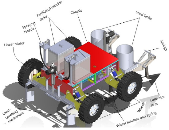
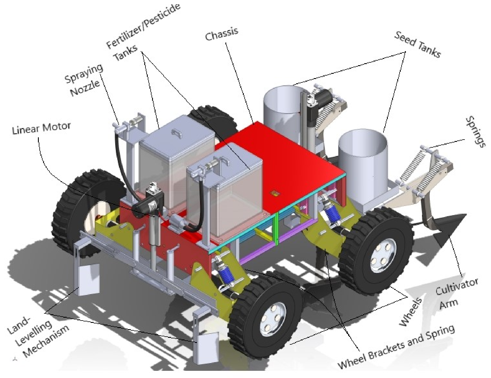
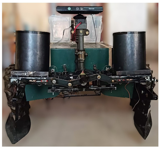
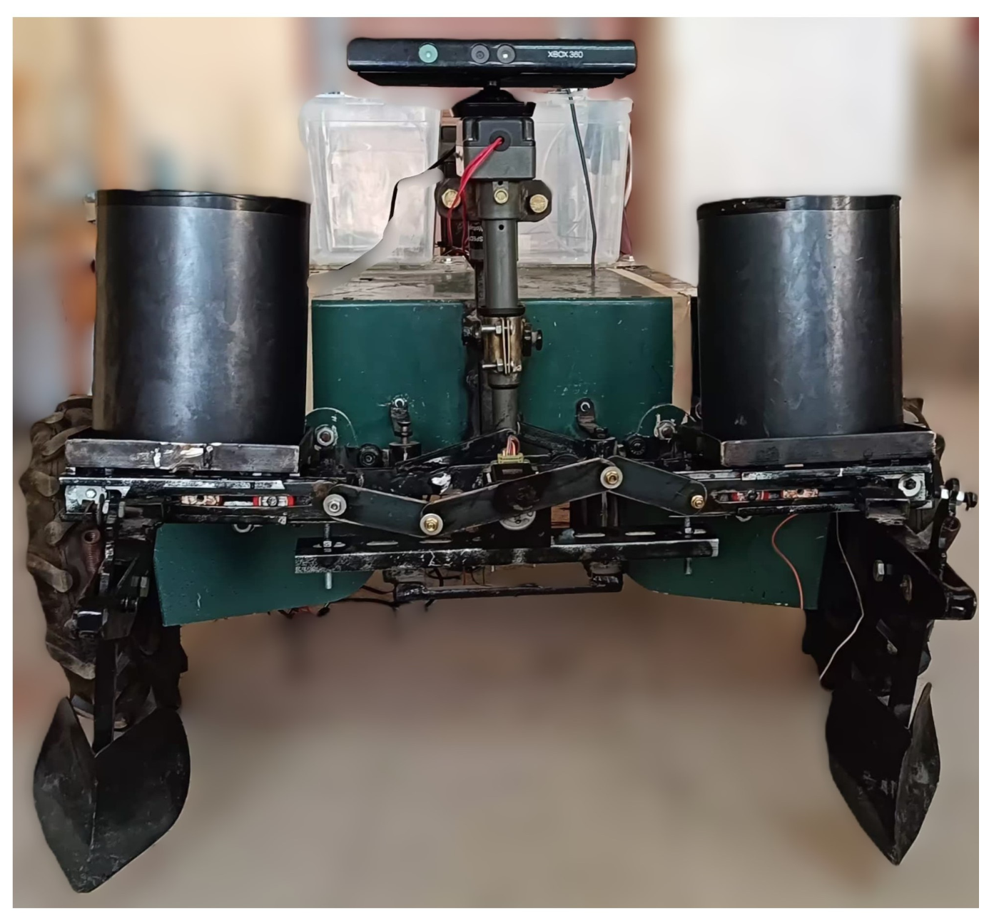
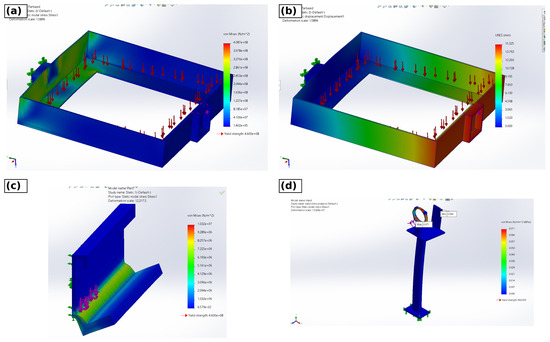
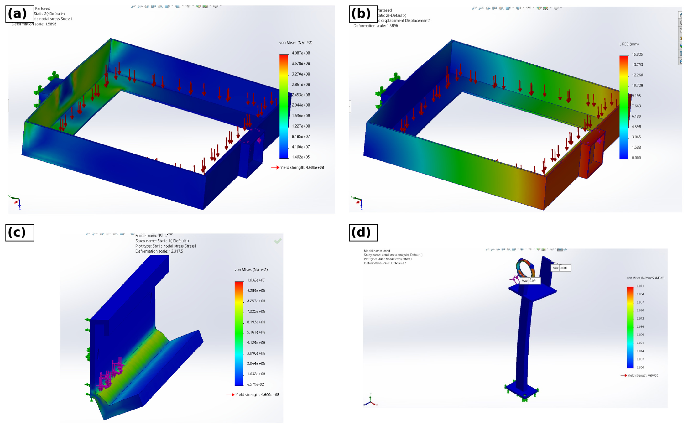
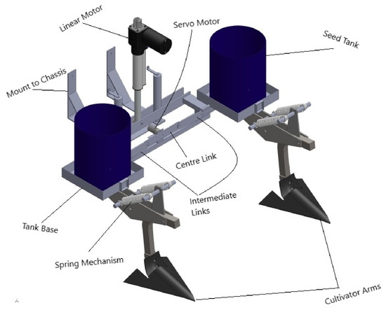
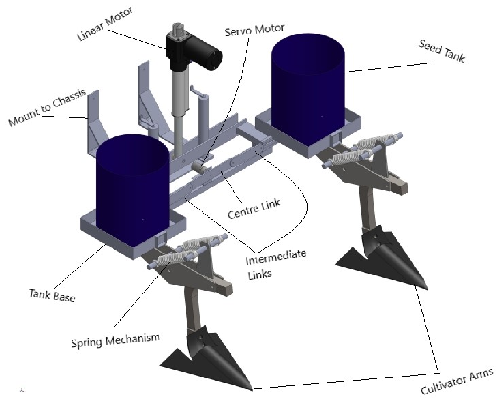
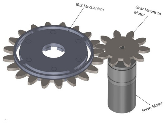
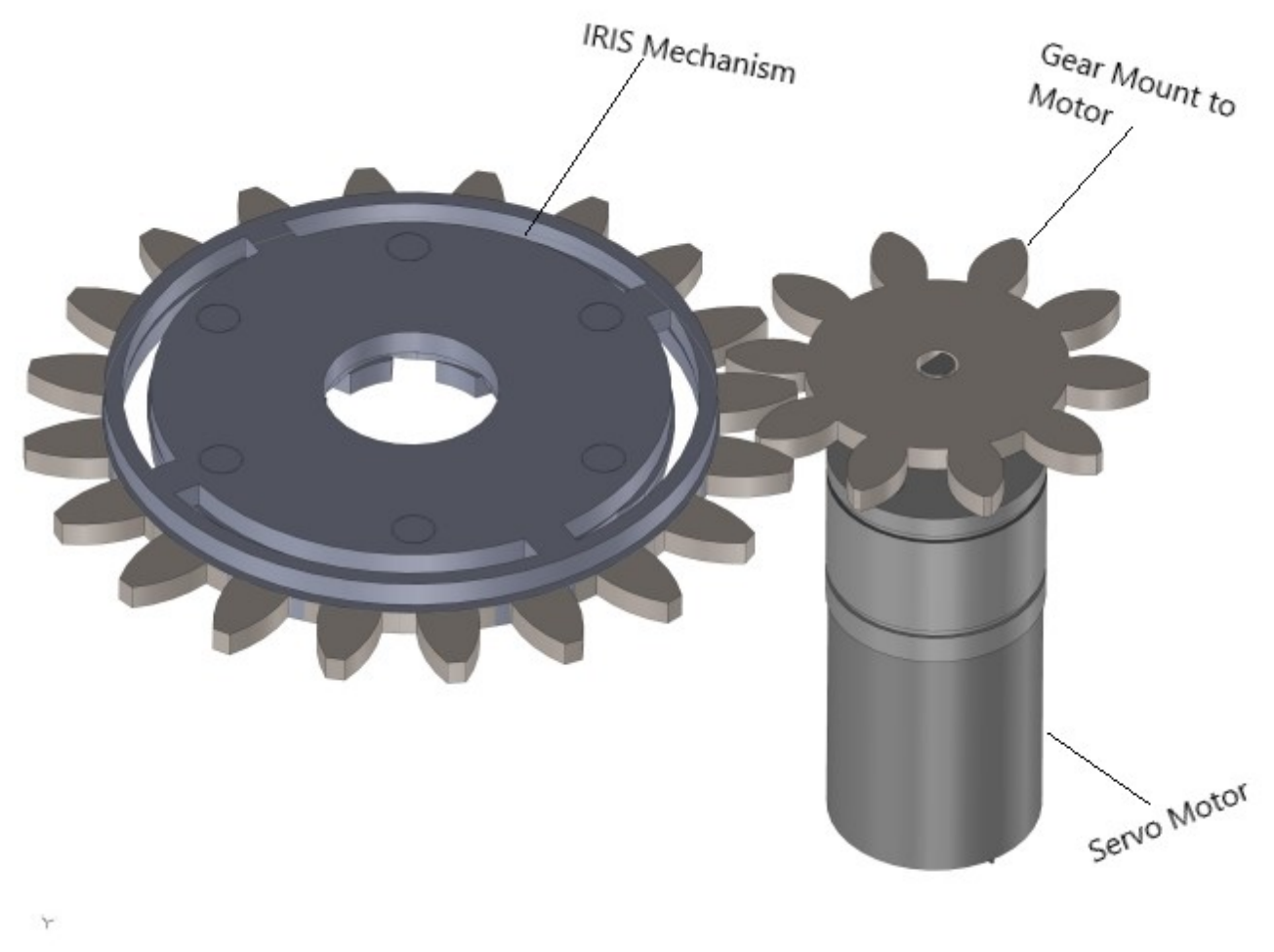
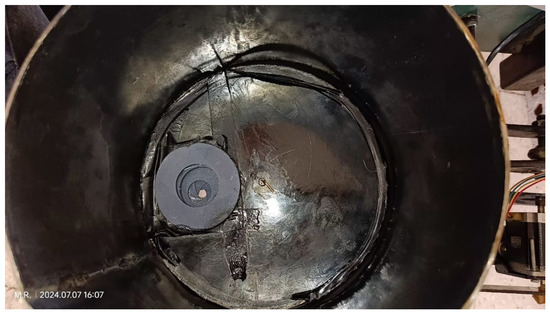
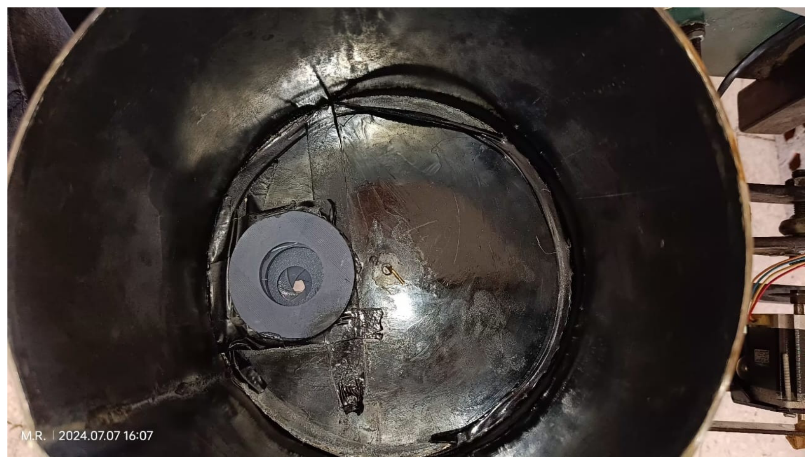
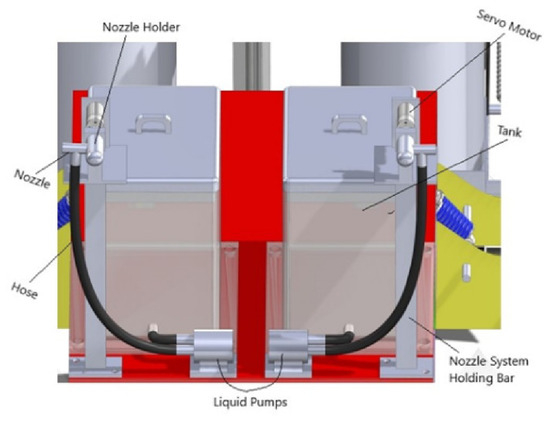
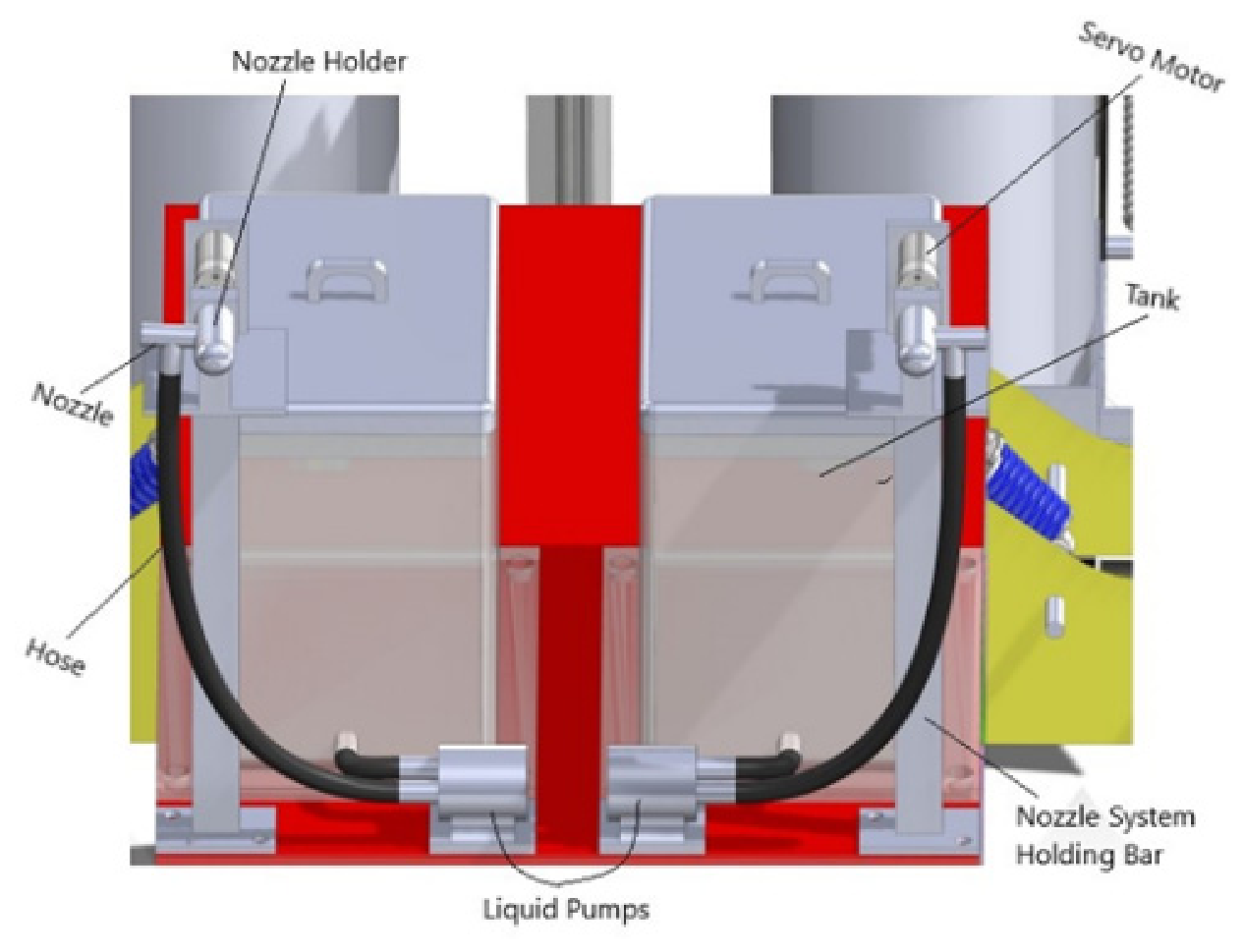
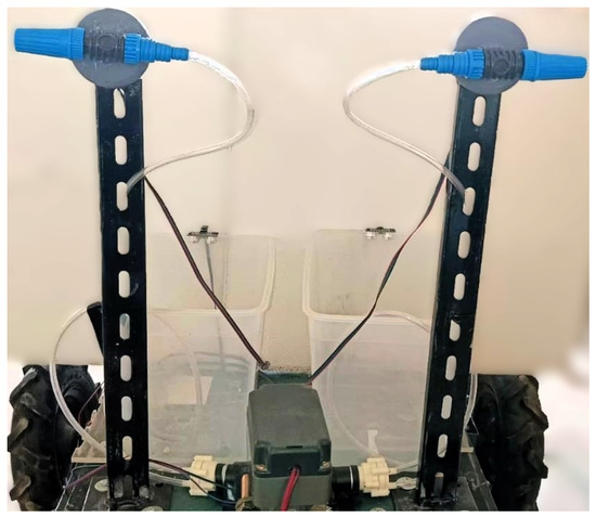
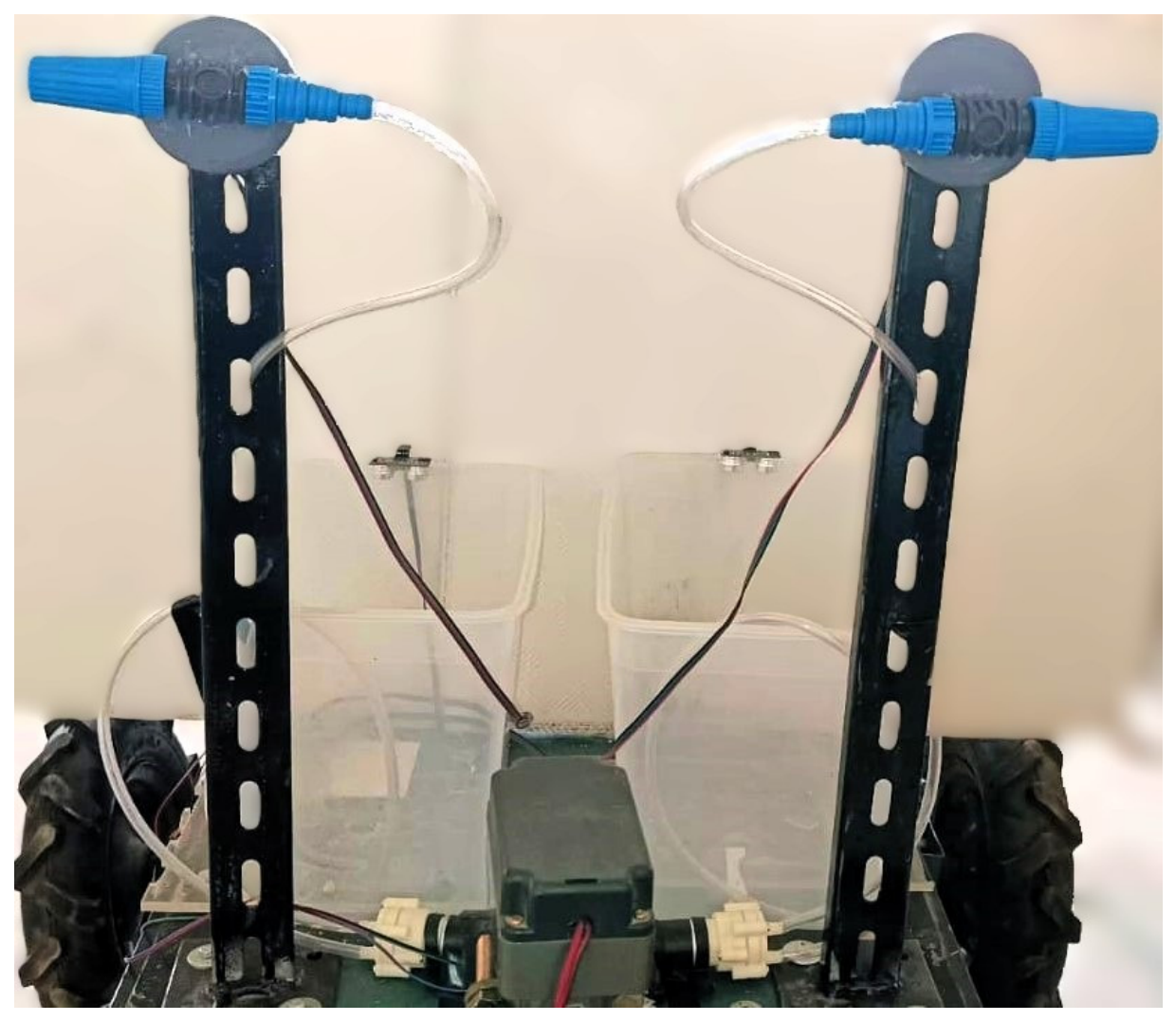
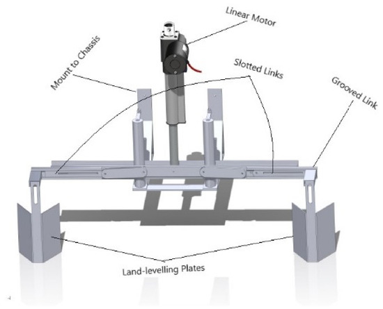
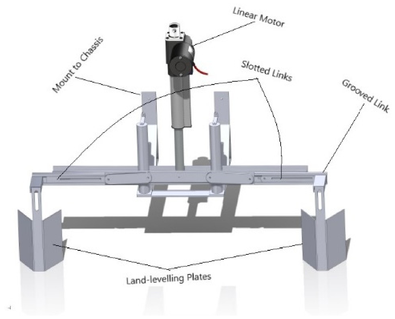
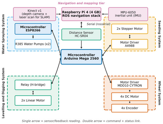
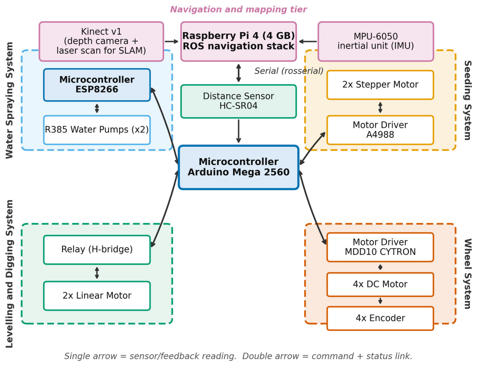
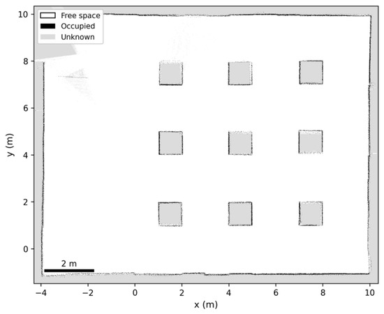
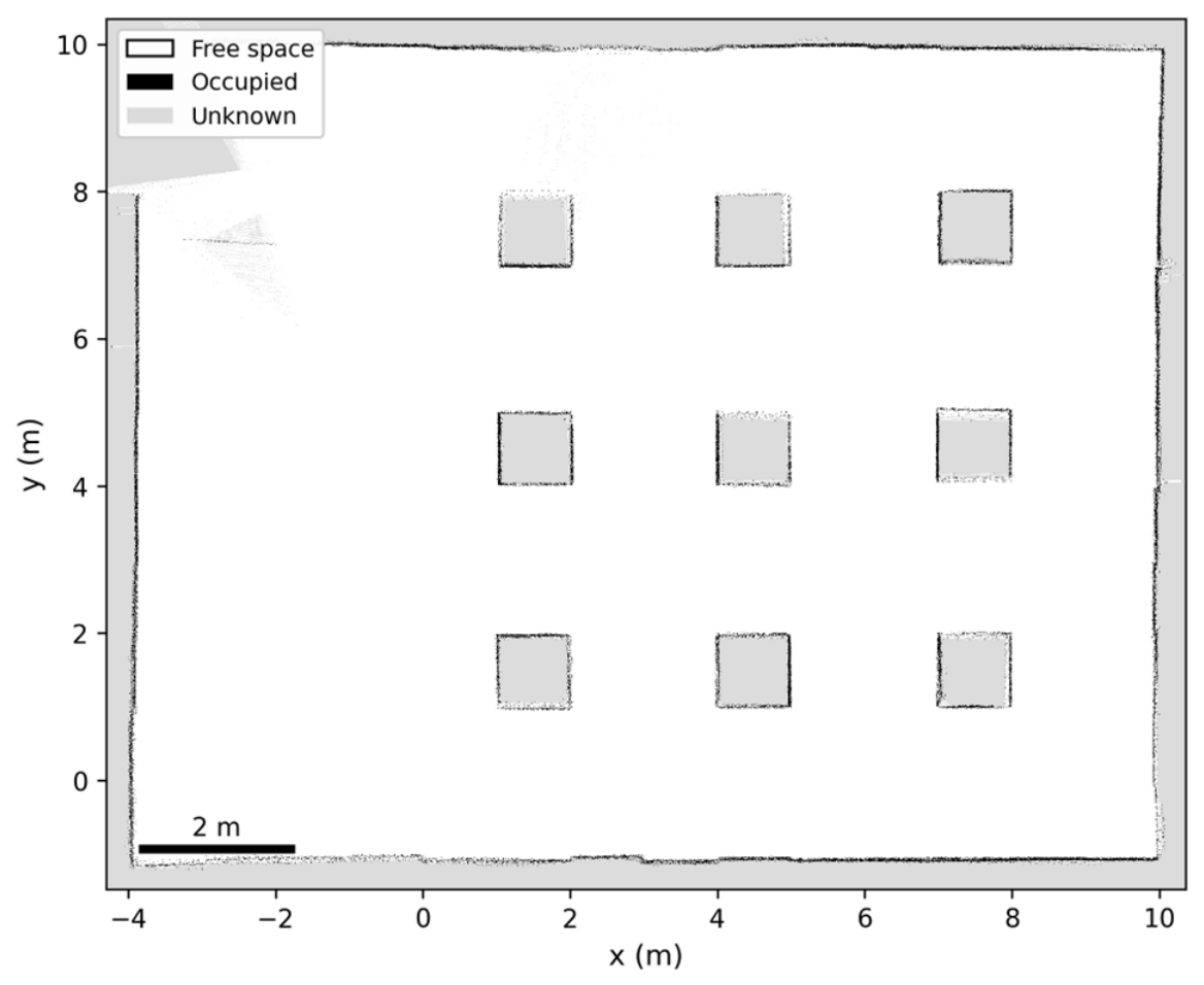
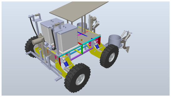
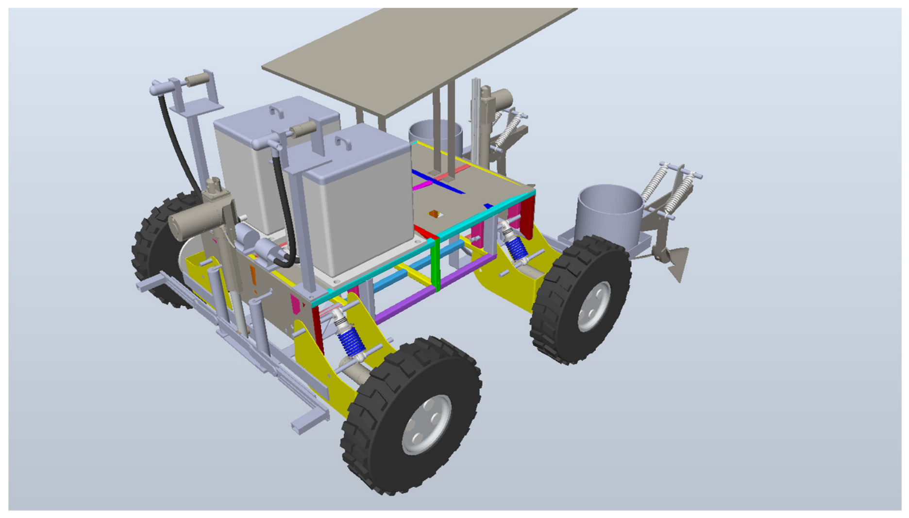
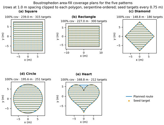
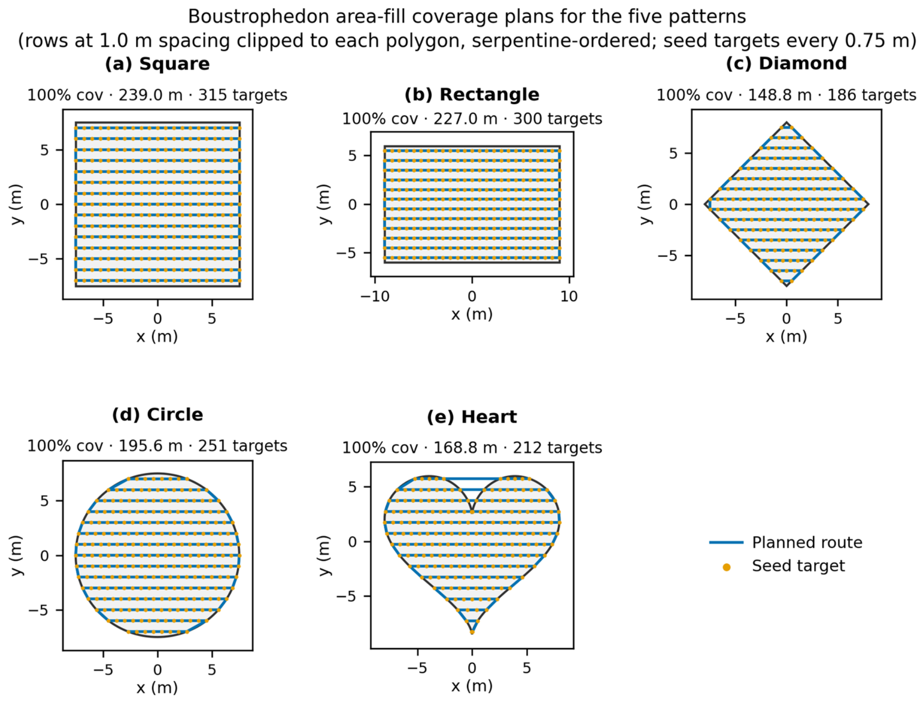
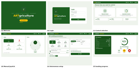
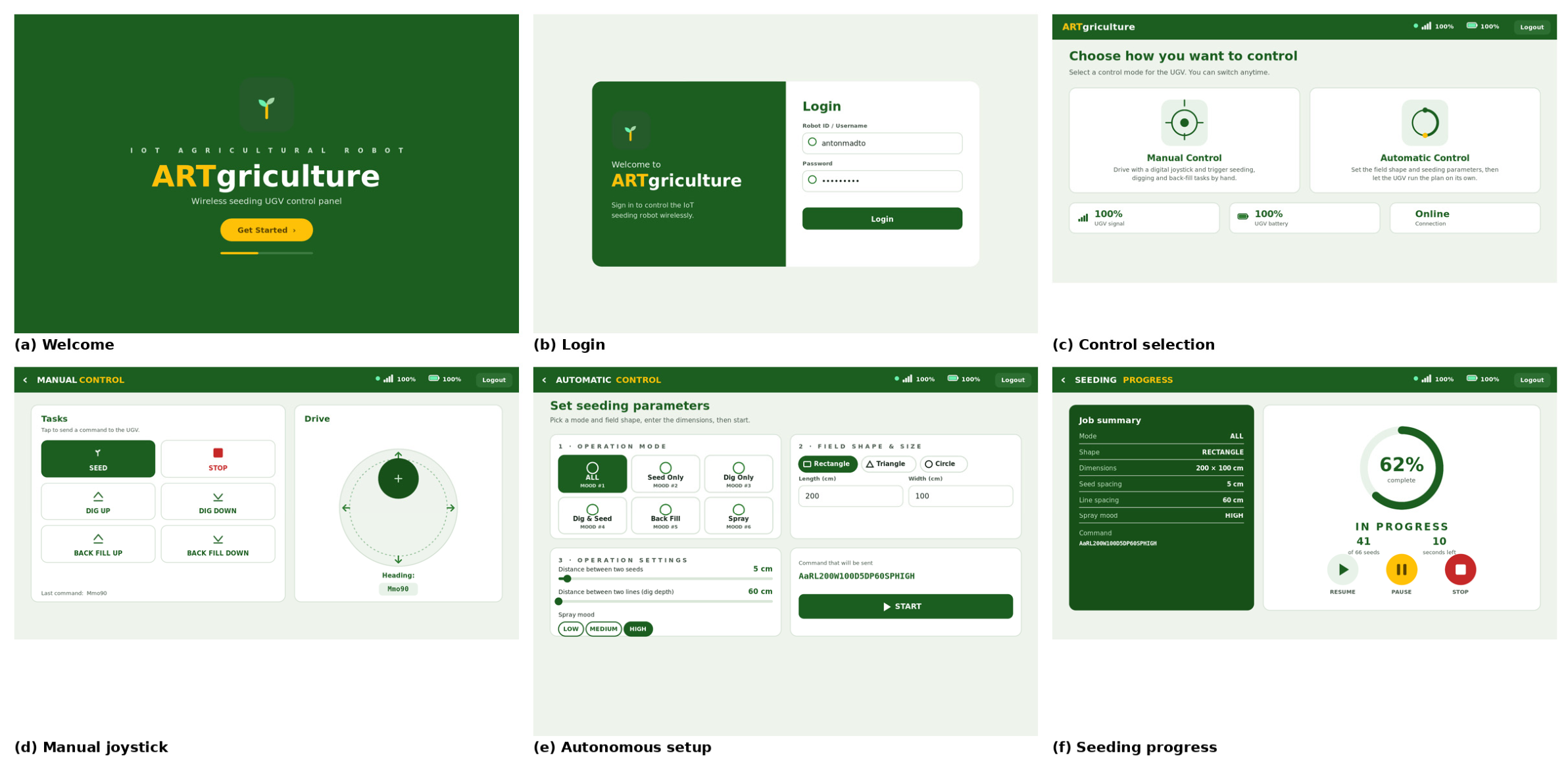
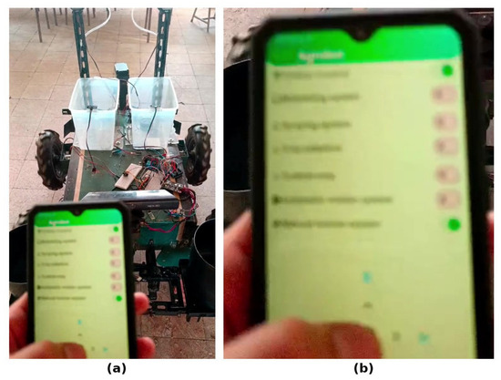
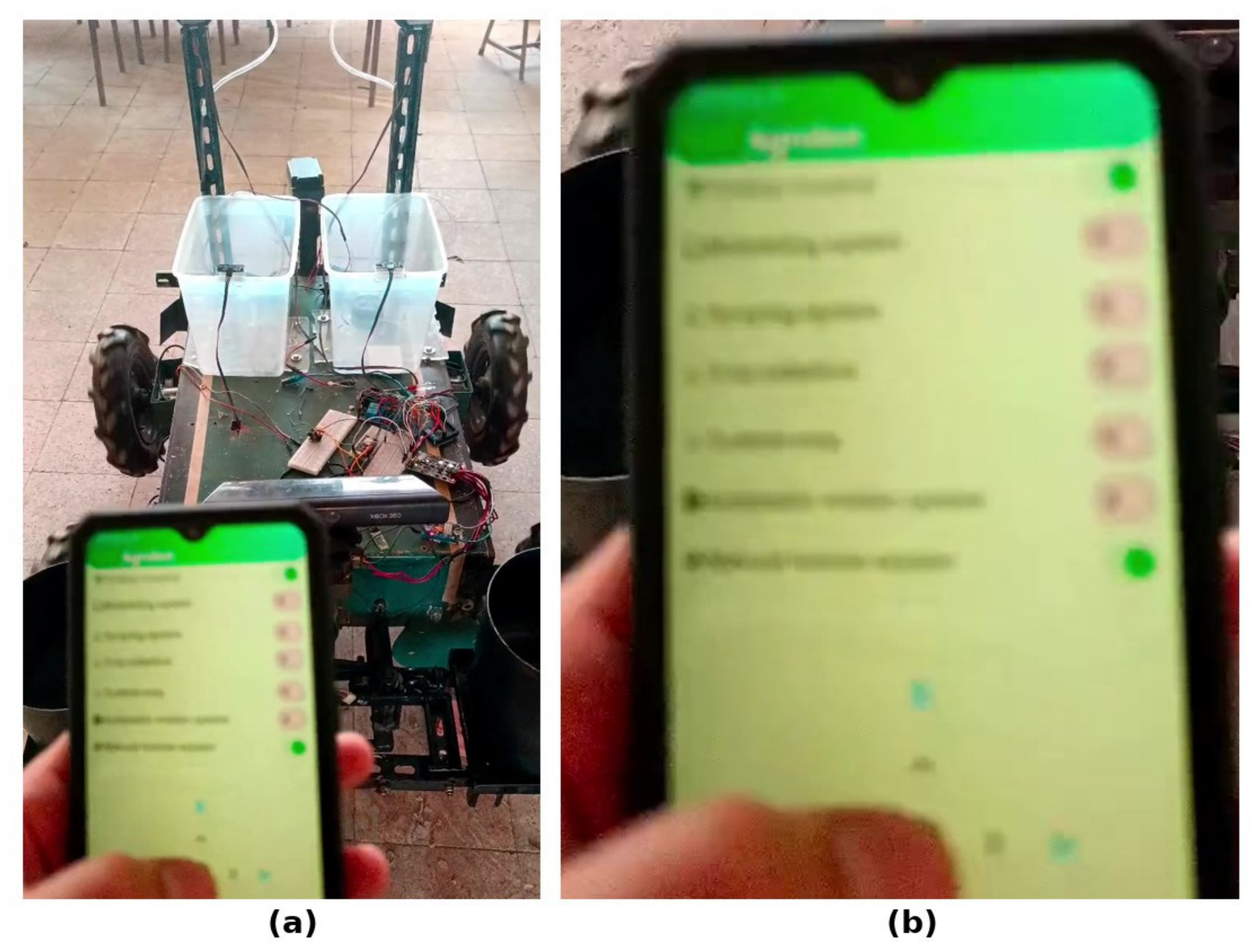
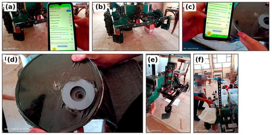
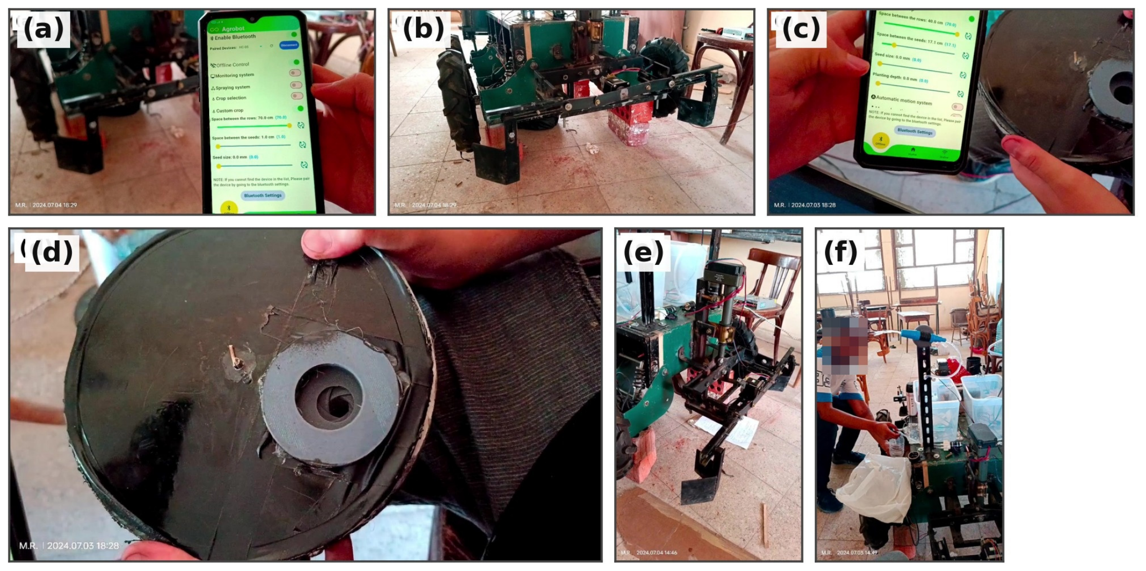
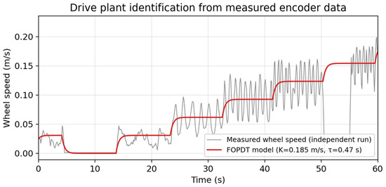
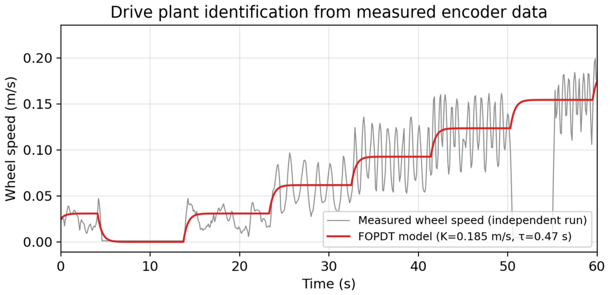
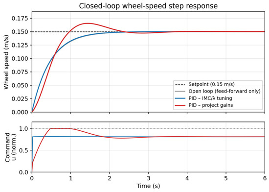
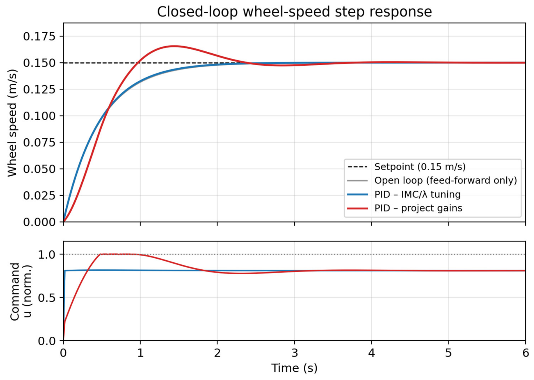
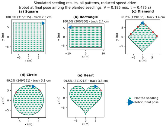
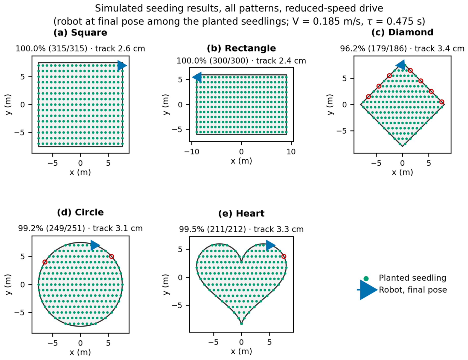
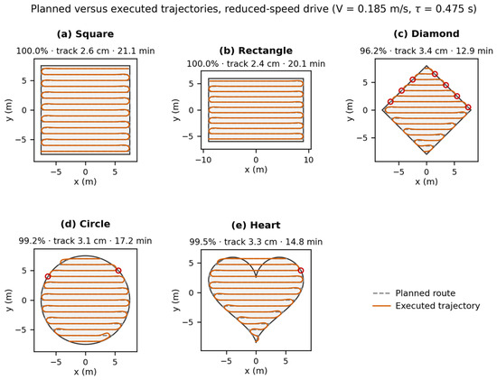
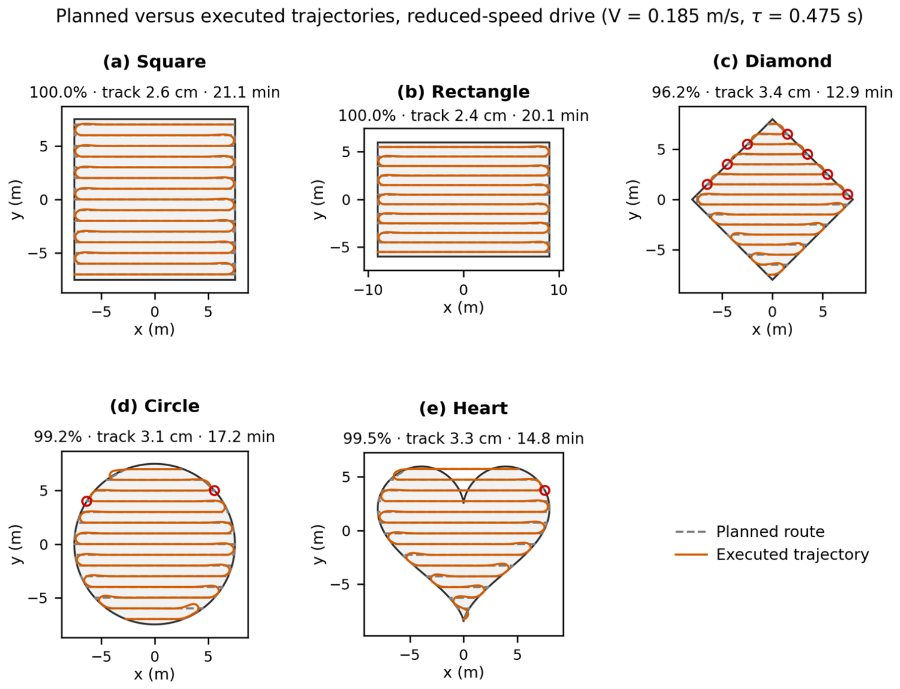
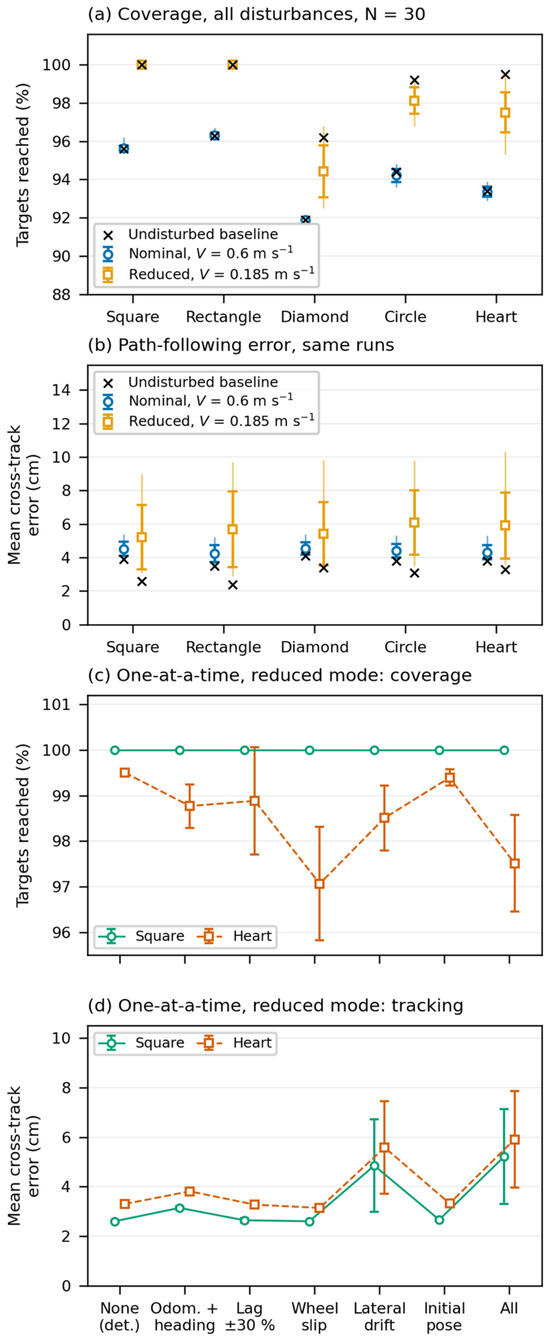
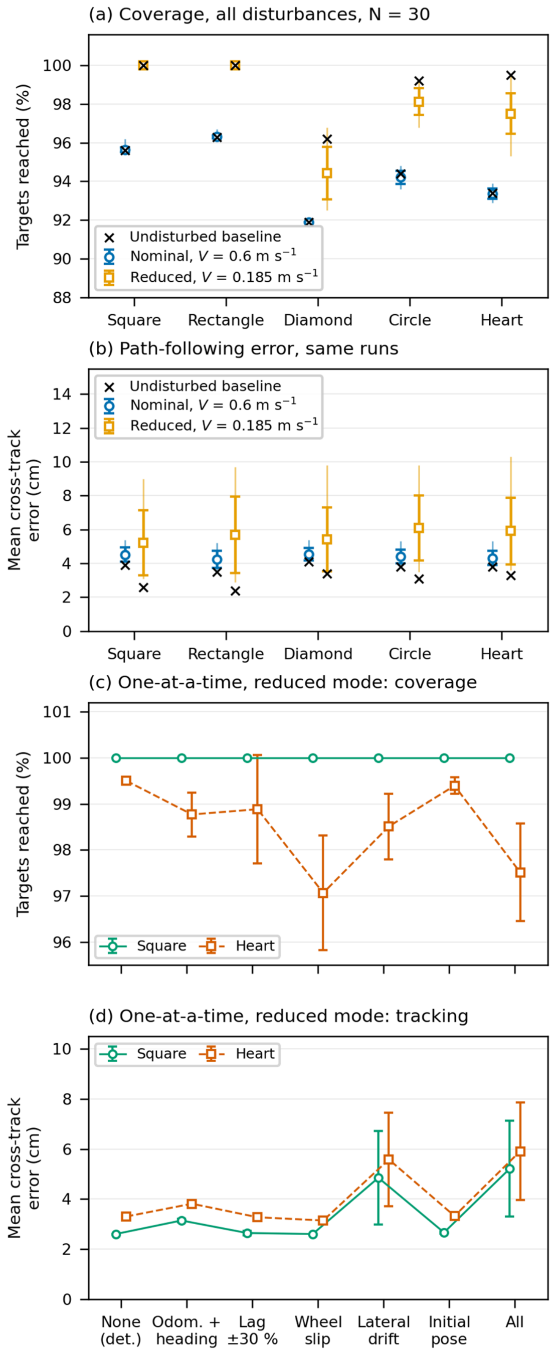
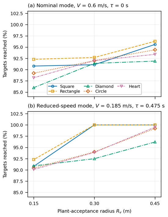
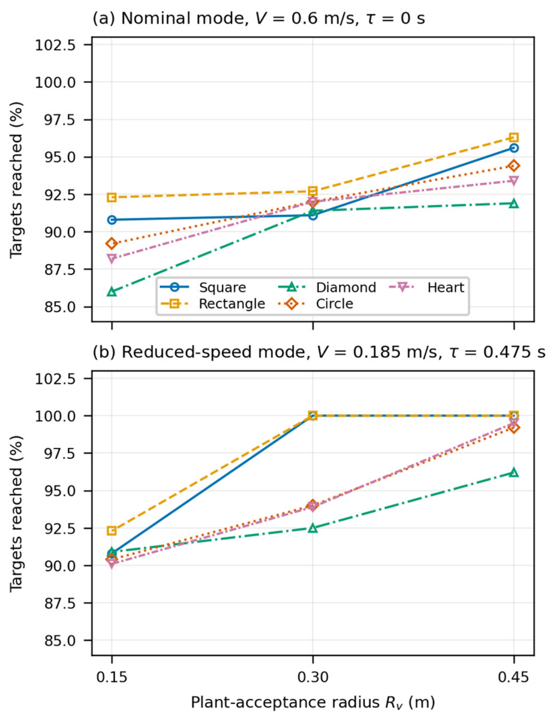

Disclaimer/Publisher’s Note: The statements, opinions and data contained in all publications are solely those of the individual author(s) and contributor(s) and not of MDPI and/or the editor(s). MDPI and/or the editor(s) disclaim responsibility for any injury to people or property resulting from any ideas, methods, instructions or products referred to in the content. |
© 2026 by the authors. Licensee MDPI, Basel, Switzerland. This article is an open access article distributed under the terms and conditions of the Creative Commons Attribution (CC BY) license.