Highlights
What are the main findings?
- Building-specific, hourly air change rates (ACRs) can be reliably estimated in dense urban contexts using lumped-parameter airflow models combined with urban aerodynamic data.
- Dynamic, context-based ACR inputs reduce prediction errors in building energy use compared to fixed infiltration rates.
What is the implication of the main finding?
- The methodology provides a scalable and computationally efficient way to improve the accuracy of Urban Building Energy Models (UBEMs).
- More realistic ventilation and energy assessments support urban planners and policymakers in optimizing energy efficiency at larger scales.
Abstract
Accurate estimation of building-specific air change rates is important for reliable urban-scale energy modeling, particularly in densely populated regions where airflow calculations must account for complex boundary conditions associated with urban geometry. This study applied lumped-parameter airflow models to simulate interzone airflow by calculating the internal pressures using simplified building representations. Air change rates were calculated by solving a system of nonlinear equations, with boundary conditions defined by localized wind inputs corrected using aerodynamic parameters extracted from three-dimensional urban geometry. By linking these wind-related boundary conditions with lumped-parameter airflow models, the methodology describes spatial variability in natural infiltration across a broad range of urban densities. Two cities were compared to test the variability in building air change rates using local boundary conditions: New York City, a dense modern city, and Turin, a typical medium-density European city. Moreover, verifying the lumped-parameter model against CONTAM (Version 3.4.0.6) showed accurate results, with a mean absolute percentage error of 1.2% across 120 simulated weather scenarios. Furthermore, comparing energy consumption predictions using building-specific air change rates to those using fixed air change rates showed improved accuracy, resulting in an average error reduction of 27% over the entire heating season for a sample building. This scalable, automated approach enables more accurate assessments of ventilation-driven energy use in compact urban areas.
1. Introduction
The accurate estimation of air change rates (ACRs) is a critical component of energy consumption models, particularly in dense urban environments where building density, surrounding topography, and local weather conditions heavily influence airflow patterns [1]. Infiltration, or the unintended airflow through building envelopes, directly impacts heating and cooling demands, which are integral to determining building energy usage [2,3]. In urban areas, infiltration rates are influenced by factors such as building geometry, surrounding environment, and local weather conditions. As urbanization increases, the variability of ACRs across buildings in a city becomes more pronounced, necessitating a more accurate, context-sensitive approach to modeling infiltration.
Several multizone airflow modeling tools, such as CONTAM, have been developed to estimate building ACRs. CONTAM, developed by the National Institute of Standards and Technology (NIST), is widely used to calculate airflow rates and assess ventilation adequacy in buildings [4]. However, the traditional use of CONTAM often assumes surface-averaged wind conditions, which may oversimplify the complex effects of the surrounding urban environment on wind patterns. This oversimplification can lead to inaccurate infiltration estimates, especially in dense urban areas.
Recent studies have emphasized the importance of accurately accounting for wind-driven infiltration, which varies widely by location and surrounding environment. Herring et al. investigated the effects of wind pressure inputs on the predicted ACR, showing that pressures on building surfaces where airflow paths are located should be specified at a resolution appropriate for the smallest volume of interest to ensure reliable results [5]. Their findings underline the importance of high-resolution input data in accurately modeling the impact of wind on building airflow. Similarly, Ng et al. noted the significance of airflow modeling for residential and commercial buildings, where real-time estimates of infiltration could improve energy management and indoor air quality control [6].
To address these limitations, tools like the Urban Multi-scale Environmental Predictor (UMEP) have been developed to provide aerodynamic parameters, i.e., roughness length (z0) and displacement height (zd), which can be used in wind speed corrections [7]. This enables a more accurate representation of wind-driven airflow around buildings for use in models like CONTAM.
Although various modeling approaches exist [8,9], the potential of lumped-parameter models (LPMs), coupled with corrected wind speed profiles for estimating building ACRs in urban contexts, has not been fully established in the literature. Prior infiltration studies often applied generalized or static assumptions for wind conditions and ACRs, overlooking the spatial and temporal variability introduced by complex urban morphologies [10]. At the urban scale, recent wind studies have highlighted the strong influence of building form and layout on local wind fields, underlining the need for more context-sensitive boundary conditions [11]. Moreover, recent reviews highlighted that this spatial variability is often insufficiently integrated into building ventilation and airflow modeling frameworks [12]. As a result, commonly used boundary conditions may not adequately represent the wind environment experienced at the building scale, particularly in dense urban settings. Thus, the present challenge is to improve ACR estimation by integrating boundary conditions that incorporate localized wind speed corrections into LPMs, enabling more accurate and context-sensitive predictions across a broad range of urban settings.
1.1. Building Airtightness Measurements
To provide context for building infiltration, this section provides a brief introduction to airtightness testing methods that can later be used to calculate leakage areas.
Whole-building airtightness measurement techniques include fan-pressurization methods (such as ASTM E779) [13]. These methods employ blower doors to establish pressure differences. After sealing intentional openings, airflow rates are monitored at different pressures to establish an airflow versus pressure curve from which a leakage coefficient (C) and exponent (n) can be determined for use in the building airflow model. This airflow–pressure relationship, governed by the resistance of the flow path, is commonly described by the power-law equation:
where Q [m3/s] is the volumetric flow rate, C [m3/s·Pan] is the flow coefficient, ∆P [Pa] is the pressure difference, and n [-] is the flow exponent.
Using the measured flow rate obtained from the test data, the leakage per unit area can be derived, as described later in the Section “Leakage Area Calculation”.
Consequently, reference infiltration values from various experimental studies [14] serve as the primary input for calculating airflow-induced building air permeability when direct data for the analyzed buildings are unavailable.
1.2. LPMs Within Urban Environments
The LPM approach, adopted in this work, is based on simplified representations of physical systems, which can make them more effective approaches for urban-scale applications than more detailed CFD models that are computationally prohibitive [15]. LPMs for airflow in multizone buildings represent a collection of zones (or volumes of air) in a building as nodes and the airflow connections between them as links. Specialized simulation tools such as CONTAM [4] and COMIS [16] implement this approach by applying physical principles to calculate airflow rates, ventilation performance, and contaminant transport within buildings.
Air within the zones is represented by homogeneous characteristics, i.e., temperature and pressure, which can vary with elevation to account for the effects of buoyancy and air speed on interzonal airflow. From a modeling standpoint, the parameters governing the dynamic behavior of the system are considered to be concentrated at discrete locations rather than continuously distributed in space. This assumption reduces model complexity while maintaining a reasonable level of accuracy, provided that the building configuration remains relatively simple [17].
Airflows attributed to natural ventilation, i.e., no mechanical ventilation, are driven by:
- wind pressures on the building façades acting on connections between interior and exterior building zones;
- buoyancy effects are attributed to differences in node density and elevation of interzone connections, i.e., stack effect.
2. Objective of the Work
This study aims to estimate ACRs of naturally ventilated buildings in realistic urban contexts, accounting for roughness elements (e.g., local terrain and surrounding buildings) and weather conditions. These improved ACR estimates are meant to support accurate and reliable analyses of building energy performance. To enable applicability at the urban scale, LPMs, which represent each building as interconnected zones, were used to calculate hourly ACRs. These hourly ACR estimates were subsequently integrated into process-driven energy models within an existing Urban Building Energy Modeling (UBEM) framework [18], which considers:
- Local weather effects, including façade-specific solar irradiation, surface temperature, and wind;
- Urban morphology, including the width of street canyons and building height;
- Building physics characteristics, including envelope thermal properties, energy system efficiency, and internal heat gains and losses.
3. Materials and Methods
To calculate building-specific hourly ACRs, the appropriate wind boundary conditions for each building were first determined based on the local urban context and weather data.
Wind speed in dense urban areas is affected by two main mechanisms. First, roughness elements surrounding openings, such as neighboring buildings and vegetation, affect wind velocities at openings in building façades. Second, airflows within street canyons display complex vortices and circulation patterns due to interactions among wind speed, canyon aspect ratio (H/W), and surface temperature differences between opposing façades. The first is addressed using aerodynamic parameters (e.g., displacement layer, zd, and roughness length, z0) with log-law or power-law wind speed profiles [19,20], while the second relies on Computational Fluid Dynamics (CFD)-derived adjustments [21]. In this work, wind speed was corrected using z0 derived from the UMEP tool within the software tool, QGIS (version 3.34.6) [22]. Wind speed correction was applied for each building based on the prevailing wind direction (for each 30°) and leakage element height.
The correct wind boundary conditions were then applied to each building represented with an LPM. These models required building leakage assumptions to account for airflow through the building envelope and interzone flows. Envelope leakage parameters were derived from airtightness tests, provided in [14], and converted appropriately for use in the LPM, as provided in the next section. Furthermore, geometric and temperature scenarios were tested to highlight their effects on whole-building ACRs, i.e., the inclusion/exclusion of roof leakage and the testing of different air temperatures within the building.
Finally, the hourly ACRs were used as inputs to an urban-scale energy consumption model and compared to energy consumption calculated using fixed ACRs. The fixed ACRs were determined based on building envelope leakage associated with the construction period [23]. Figure 1 illustrates the general methodology.
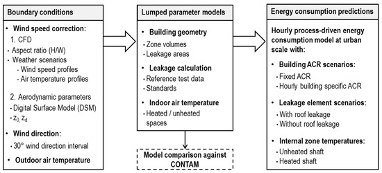
Figure 1.
General methodology.
3.1. Data Sources and Normalization
Table 1 provides sources of building envelope leakage data. Infiltration metrics reported across these sources may use different units and test conditions, so the following example shows how to calculate the effective leakage area from test data. In this work, the data from the RDH report were used.

Table 1.
Leakage area references.
Leakage Area Calculation
Effective leakage area (ELA) is used to quantify the area of openings in a building envelope as a single opening that would result in similar airflow under driving forces such as those imposed during envelope leakage testing. Calculating these parameters involves converting measured airflow rates into equivalent leakage areas, typically referencing standard air density. Having a measured test airflow rate, QT, determined at desired test conditions (see Equation (1)), ∆PT, it is possible to calculate the leakage per unit area in cm2/m2 as follows:
- ○
- Convert the flow at test pressure and power-law exponent to the flow at desired reference pressure difference:
- ○
- Calculate ELA per unit envelope surface area:
ELA = effective leakage area per envelope surface area [cm2/m2];
QT = airflow at test pressure [m3/s·m2];
Qr = airflow at reference pressure [m3/s·m2];
Cd = discharge coefficient, 1.0 [-];
= power-law exponent, 0.65 [-];
= standard air density = 1.2041 at sea level and 20 °C [kg/m3];
ΔPT = test pressure difference [Pa];
ΔPr = reference pressure difference [Pa].
As presented here, ELA was used to quantify the total leakage area (AL) associated with each flow path, based on the path’s surface area (As [m2]); AL = ELA × As.
3.2. LPM Approaches
Figure 2 illustrates the LPM layout with two modeling approaches (vertical sections) and the associated system of nonlinear equations. Each building is represented as three (3ZLPM) or four (4ZLPM) zones (a, b, and c) connected to the outdoors (at external pressure nodes 1–4) through connections in the street canyon and opposite façades (typically a courtyard in Italian buildings evaluated here).
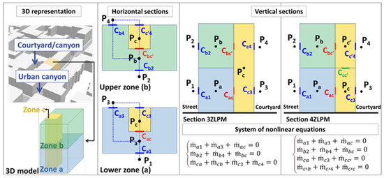
Figure 2.
Detailed schematic of the LPM: “zone a” in blue (lower apartments’ level), “zone b” in green (upper apartments’ level), and “zone c” in yellow (vertical shaft).
3ZLPM and 4ZLPM differ in their shaft modeling assumptions: 3ZLPM represents the shaft with a single pressure at mid-height, while 4ZLPM uses two pressures located at the upper and lower ends of the shaft. Zones a and b are not directly connected to each other in any configuration.
This three/four-zone simplification enables effective, city-scale modeling while maintaining sufficient accuracy for low- to mid-rise buildings (up to sixteen stories) as validated in a previous work [17], which confirmed that the simplified three-zone model provides an acceptable level of accuracy in predicting whole-building ACRs when compared with a detailed building model.
Table 2 provides the volume and temperature assumptions made for each of the three zones. If the net heated building volume is not known from the building database, which usually only provides the building’s footprint area, the gross volume is obtained by multiplying the footprint area by the building height. The net heated volume is then estimated as 70% to 75% of the gross volume; in this study, a factor of 0.75 was applied. This follows a common “rule of thumb” and is consistent with the Decree of 26 June 2009 on national guidelines for the energy certification of buildings, which, in Annex A, states that, in the absence of specific data, the net heated volume can be assumed as 70% of the gross volume [26]. Here, net refers to the heated volume of the building, excluding the space occupied by internal partitions.
Table 2.
Simplified building zoning and air temperature assumptions.
Table 2.
Simplified building zoning and air temperature assumptions.
| Zone a | Zone b | Zone c | ||
|---|---|---|---|---|
| Description | Lower Apartment | Upper Apartment | Shaft | |
| Volume (a & b) [m3] | (net heated volume − shaft volume)/2 | net footprint shaft area (known or based on construction period) × net building height | ||
| Air temperature [°C] | Winter | Tia = 20 | (Toa is provided in Table 3) | |
| Summer | Tia = 26 | |||
Table 3.
Tested weather scenarios for model verification.
Table 3.
Tested weather scenarios for model verification.
| Winter | Summer | |||||||||
|---|---|---|---|---|---|---|---|---|---|---|
| Toa [°C] | −10 | −5 | 0 | 3 | 7 | 12 | 24 | 28 | 30 | 34 |
| U [m/s] | 0.1, 0.5, 1 to 10 (with an increment of 1 for each simulation) | |||||||||
As for the shaft area and building height, it was treated similarly: the net footprint shaft area/building height means that the wall/slab thicknesses were excluded from the calculation. The indoor air temperatures (Tia) for the heated zones were assumed to be setpoint temperatures of 20 °C in winter and 26 °C in summer. The shaft (zone c) was assumed to be unheated; thus, its temperature (Tsh) was calculated, as presented in Table 2, based on the indoor and outdoor temperature (Toa) and a correction factor (btr,u) of 0.4, according to the standard UNI/TS 11300-1:2014 [27] for confined spaces.
The mass balance in each zone can be described as:
where each mass flow rate, [kg/s], follows a power-law relationship with pressure difference ∆Pij (Pi − Pj) and exponent n, thus resulting in a non-linear set of equations with respect to the unknown internal pressures (Pa, Pb, and Pc) represented in Figure 2. This system of nonlinear equations was solved using MATLAB (version R2023b) [28].
The leakage area for each analyzed airflow path, AL [m2], was calculated using an ELA of 2.642 cm2/m2 (∆Pr = 4 Pa, Cd = 1, n = 0.65), which was obtained by converting the mean value for masonry buildings, QT = 4.58 L/s·m2 @ ∆PT = 75 Pa [14], using Equations (2) and (3).
Connections between the shaft and the two zones, a and b, were modeled as closed doors (highlighted in red in Figure 2), each having a leakage area of 45 cm2 (assuming a 90 cm wide door with a 0.5 cm high undercut). To scale this leakage to the full building height, a multiplier was applied based on the assumption that each floor has two apartments, and the resulting value was used as the multiplier for the number of doors.
The LPMs were also defined to include roof leakage to assess the difference in the ACRs. Also, the shaft temperature was set using the equation for Tsh provided in Table 2 and equal to the heated zone temperatures, Tia, presented in Table 2, to highlight the effect of internal temperatures on building ACRs.
Finally, to compare the LPMs with CONTAM models, a set of outdoor air temperature (Toa) and wind speed (U) scenarios was selected as provided in Table 3. The wind speed values ranged from 0.1 m/s to 10 m/s, covering 12 discrete scenarios, and were combined with 10 representative outdoor temperature conditions. This resulted in a total of 120 distinct boundary-condition scenarios used for the comparison. The inclusion of both mild and extreme sets of ambient conditions (i.e., 10 m/s, −10 °C, or 34 °C) ensured the robustness of the model evaluation across a range of weather conditions.
3.2.1. Boundary Conditions Used for the LPMs
To define the correct boundary conditions for infiltration models, wind velocity should be corrected at the façade level. This adjustment requires correcting wind speed from the reference weather station to the building scale, where the displacement level (zd) [m]—the height above ground at which zero-plane wind speed is assumed due to the presence of obstacles such as buildings and vegetation—plays a critical role. When the building height is above zd, the flow is less affected by near-ground turbulence, and simplified approaches such as power-law profiles are generally sufficient for wind speed correction.
When the building height is below zd, two correction methods can be applied:
(1) Computational fluid dynamics (CFD)-derived adjustments that provide more accurate vortices and flow dynamics within the street canyon [21], although these are computationally demanding and therefore usually applied only to representative canyon aspect ratios (H/W) and weather scenarios;
(2) Simplified aerodynamic approaches that use parameters such as zd and z0 within log-law or power-law profiles, suitable for large-scale urban analyses.
Table 4 summarizes these two wind velocity correction approaches and their implementation details.
Table 4.
Wind velocity correction methods.
In this work, the correction of wind velocity for the four external leakage points used a logarithmic law [19,20] with the aerodynamic parameters derived from the UMEP plugin within QGIS (i.e., z0). UMEP provides aerodynamic parameters based on real urban geometry (DSM) and the specified grid size and wind direction. These parameters, in turn, enable accounting for the real urban environment around each analyzed building, which depends on local urban roughness and prevailing weather conditions. While this method simplifies wind dynamics within street canyons, it enables urban-scale analysis by incorporating the actual surrounding urban context of the analyzed building.
At each simulated timestep, the reference wind speed Uref [m/s] is used to calculate the corrected wind velocity vcorr [m/s], which accounts for the surrounding roughness elements for a given façade opening. A logarithmic law is applied when the undisturbed wind speed exceeds 4 m/s [20] while a simple correlation model is used for lower wind speeds [19]. Having νcorr, it was possible to obtain the wind speed modifier coefficient (Ch) [-]. The wind pressure profile, f(θ), a function of the relative wind direction, is calculated knowing the hourly wind azimuth angle (θw) [°] and façade azimuth angle (θs). This wind pressure profile is calculated for each 30° wind direction interval.
These corrections provide building-specific wind pressure profiles for each opening on the building façade. Consequently, four wind pressure profiles, each accounting for a different local roughness element, were provided to the infiltration model to determine the dynamic pressure Pdyn [Pa] at the four external leakage points.
3.2.2. Input Data and Case Studies
Two case studies were selected as presented below. By applying the methodology to two cities that differ in geometry and weather, this comparison seeks to illustrate the effect of location-specific building ACR. The Turin case included data from 27 residential buildings obtained from a local utility, enabling comparisons between simulated and measured consumption.
- ▪
- Mid-Sized European City (Turin, Italy)
- –
- Residential buildings, from low- to high-density neighborhoods:
- –
- Geometry: building footprints and 3D urban environment from DSM layers [30];
- –
- Weather data: local meteorological observations for 2022–2023 (e.g., air temperature, wind speed, solar irradiation) [31];
- –
- Measured energy data: hourly space-heating consumption from the local district-heating provider [32].
- ▪
- New York City (NYC), USA
- –
- Residential buildings situated within high-density street canyons (Manhattan):
- –
- Geometry: detailed building vectors from municipal technical maps [33] and a 3D urban environment from LiDAR-derived DSM [34,35];
- –
- Weather data: urban weather station time series (Typical Meteorological Year) [36];
- –
- Measured energy data: not applicable.
The average monthly outdoor air temperature (Toa) and wind speed (Uref) for both cases are presented in Table 5.
Table 5.
Monthly average outdoor air temperature and wind speed.
4. Results
This section presents the results of the analyses outlined in the previous sections. Section 4.1 reports the results of UMEP and the corrected wind velocity for the four external leakage points. Section 4.2 compares the performance of the LPM approaches, 3ZLPM and 4ZLPM, against CONTAM. Section 4.3 provides the application of wind speed correction and the resulting building ACR based on the effect of different urban contexts, Turin and NYC, enabling the assessment of how urban morphology influences building infiltration.
Section 4.4 explores a series of scenarios that vary in roof and internal temperature settings to investigate the LPM’s sensitivity to input conditions.
Finally, Section 4.5 demonstrates the integration of building-specific ACR values into an hourly process-driven energy consumption model and compares the results with those obtained using a fixed ACR, using the 27 buildings in Turin with measured hourly energy consumption.
4.1. Wind Speed Correction
An example of the aerodynamic parameters derived from UMEP as a function of the 3D urban environment and the prevailing wind direction is provided in Figure 3 for the roughness length (a) and displacement height (b). The grids had a resolution of 5 m × 5 m, and for each grid cell, a 200 m search radius was applied to identify surrounding roughness elements. The figures illustrate the variation in z0 and zd for two example prevailing wind directions, 30° (left) and 120° (right), and highlight the influence that the surface roughness elements have on the magnitude of z0 and zd for these two wind directions.
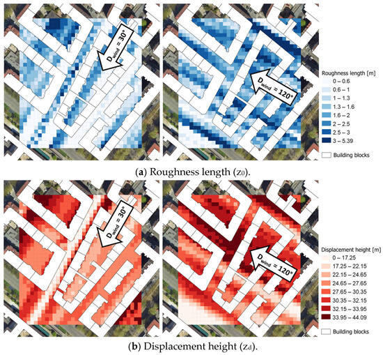
Figure 3.
UMEP results for wind-direction-specific z0 (a) and zd (b).
These wind-direction-specific z0 and zd values are two of the main parameters used to correct the reference wind speed (Uref) to façade-specific wind velocities.
Figure 4 presents the reference wind speed (Uref, dotted line) and the corrected wind velocities (v1 through v4, blue and red lines) at the four points on the façade of the LPM (see Figure 2).
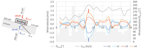
Figure 4.
Hourly wind velocities for the four openings on the façade; blue for canyon/street façade, red for courtyard/opposing façade.
Grey bars indicate the hourly prevailing wind directions recorded at the reference station [31]. Under northeast wind conditions (0–60°), points 1 and 2 showed negative corrected wind velocities (blue arrow), indicating a leeward façade at these hours, while points 3 and 4 were positive (red arrows), indicating a windward façade. Additionally, the corrected wind velocity depends on the elevation of each opening (lower: 1 and 3 vs. upper: 2 and 4), reflecting the height-dependent wind speed modifier coefficient (Ch).
The corrected wind velocities (νcorr) at the analyzed points were used to determine the building-specific Ch and the wind pressure profile (f(θ)) (using Equations (7) and (8)) for the four external façade points. These parameters served as input for the LPMs presented in the following section.
4.2. LPM Comparison
Figure 5 illustrates building ACRs for the tested weather scenarios (provided previously in Table 3). Each segment along the x-axis in Figure 5a provides the results of the wind speeds analyzed under the ten different temperature scenarios. To enable closer analyses, three wind speed cases are highlighted: 0.1 m/s in Figure 5b, 3 m/s in Figure 5c, and 10 m/s in Figure 5d. The percentage error is provided in the zoomed-in (Figure 5b–d) for each scenario in green (for 3ZLPM) and blue (for 4ZLPM).
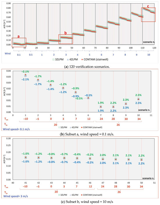
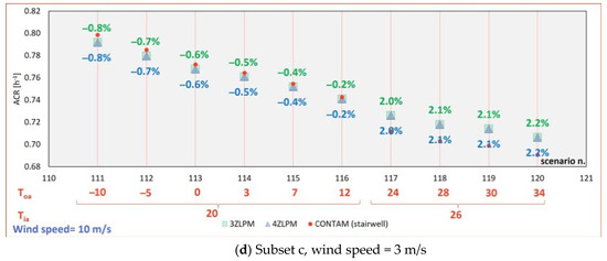
Figure 5.
Air change rate comparisons of the different LPMs under various weather conditions: (a) 120 test scenarios, (b) wind speed = 0.1 m/s, (c) wind speed = 3 m/s, (d) wind speed = 10 m/s.
The consistency between 3ZLPM and 4ZLPM is due to the large opening used to connect the upper and lower shaft, which results in a negligible resistance to airflow between the upper and lower parts of the shaft. Consequently, both models showed identical results to those obtained from CONTAM, given CONTAM’s established validity through software robustness and laboratory experiments [26,27].
The analyses under varying wind speeds revealed that model discrepancies were slightly higher at lower velocities (i.e., 0.1 m/s, Figure 5a), where airflow is primarily driven by buoyancy effects, i.e., the differences between indoor and outdoor temperatures. The average Mean Absolute Percentage Error (MAPE) with 0.1 m/s was 1.7%. As wind speed increased, wind-driven effects dominated, leading to higher convergence between both models and CONTAM (i.e., 10 m/s, Figure 5c), with an average MAPE 1.1%.
4.3. Corrected Wind Speed and Building ACR in Different Urban Contexts
Since 3ZLPM and 4ZLPM yielded similar results, the former, with a single shaft zone, was selected to simulate building ACR across varying urban configurations and assess the influence of urban morphology on ACR outcomes.
Figure 6 illustrates building density (BD) maps for two urban contexts: Manhattan, a high-density area of NYC (a), and Turin, a city with medium-to-high-density (b), where building density refers to the total building volume within a district divided by its surface area. Each map presents two selected buildings (NYC1, NYC2, TRN1, TRN2), for which the displacement height (zd) was derived using 1 m precision DSM within UMEP and a search radius of 200 m. When paired with the accompanying satellite images, these maps highlight how surrounding building heights and wind directions affect the local aerodynamic environment, determining the boundary conditions for the infiltration model.
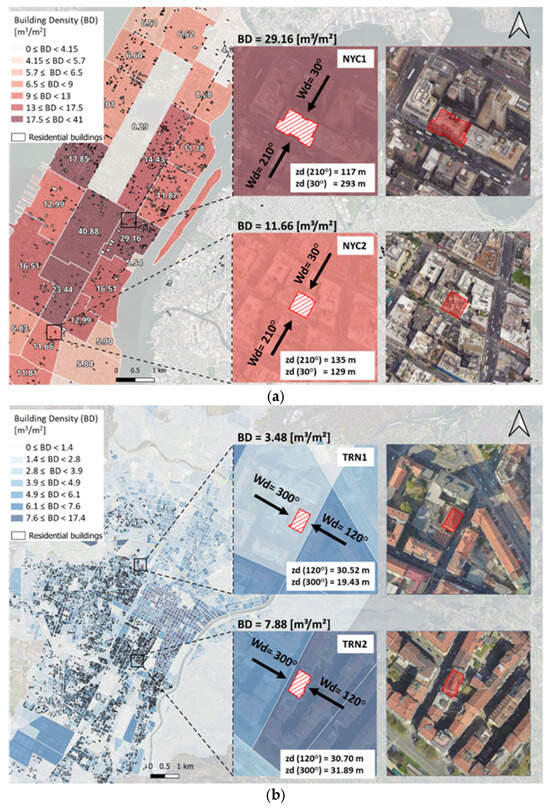
Figure 6.
Building density and zd for different urban contexts: (a) NYC and (b) Turin.
Figure 7 presents the average building ACR and wind speed (Uref) in January as a function of wind direction for the two analyzed buildings in NYC (a) and Turin (b).
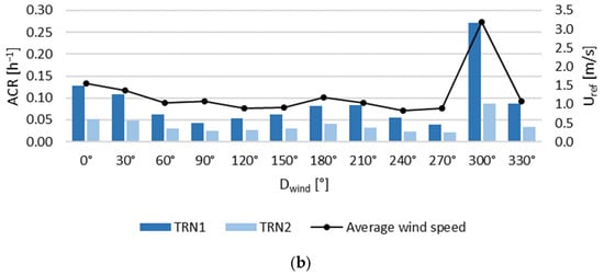
Figure 7.
Average ACR and reference wind speed in January for each wind direction interval for the two analyzed buildings in: (a) New York City and (b) Turin.
In NYC, the two buildings exhibited similar trends, with higher infiltration observed when the wind direction was parallel to the building orientation. However, the high-density urban context surrounding the buildings substantially increased the zd reducing infiltration, regardless of high wind speeds. While in Turin, TRN1 (with BD = 3.48 m3/m2) showed higher infiltration compared to TRN2 (BD = 7.88 m3/m2). For TRN1, a particularly high ACR occurred when the wind blew from 300°, which can be attributed to both the higher average wind speed from that direction and the absence of roughness elements, as indicated in the satellite imagery in Figure 6 (large courtyard).
When comparing NYC and Turin more broadly, Turin showed higher infiltration despite its lower wind speeds. This outcome is primarily due to its more open, less dense urban morphology with lower zd, combined with lower-volume buildings, which facilitate higher ACRs than the denser building configuration in NYC.
Overall, the analysis of these contrasting urban contexts demonstrates that correct wind pressure calculations should incorporate both local urban roughness and façade orientation when accounting for building-specific wind speed corrections.
4.4. Effect of Internal Temperatures and Roof Leakage on TRN2 ACR
Figure 8 presents the hourly ACRs for two example days, illustrating the influence of the difference between indoor air (Tia) and outdoor air (Toa) temperatures on infiltration, with an average wind speed of 1.1 m/s, average Toa = 22.6 °C on 4 September and −0.5 °C on 11 December. When the shaft temperature equaled the heated zone temperature, ACR(Tsh = Tia), the mean daily ACR increased by 38% in December and 17% in September compared to the shaft temperature correction provided in Table 2, ACR(Tsh). The larger difference between indoor and outdoor air temperatures in December led to greater variations in hourly ACRs compared to September. These results indicate that LPMs should incorporate the correct indoor setpoints for the shaft to better account for whole-building airflows.
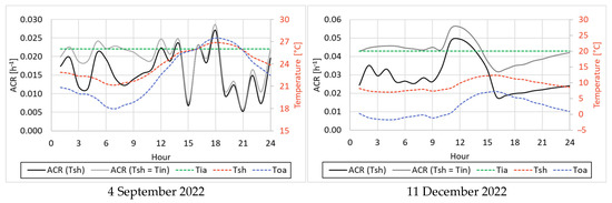
Figure 8.
Hourly building ACR with different shaft temperatures.
Moreover, implementing roof leakage into the LPM further increased the predicted ACR. Figure 9 shows the hourly building ACRs with and without roof leakage for 10 January, indicating a 48% increase in the average daily ACR when roof leakage is included. However, roof leakage should be considered only in buildings with occupied or conditioned spaces directly beneath the roof. In cases where the attic or void space is unoccupied, roof leakage may be neglected, particularly in urban-scale ventilation studies where simplifying assumptions are essential.
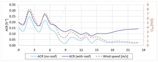
Figure 9.
Hourly building ACR with/without roof leakage.
Together, these two analyses demonstrate that leakage elements and temperature setpoints significantly affect predicted building ACRs, thereby influencing energy consumption predictions.
4.5. Hourly Energy Consumption Prediction with ACR Scenarios
For the buildings in Turin, the hourly building-specific ACRs were incorporated into a UBEM using a process-driven energy consumption model that describes the building using three thermodynamic systems (opaque envelope, windows, and building interior) [18]. Figure 10 presents the space-heating energy consumption (EC) and heat loss due to ventilation (Qv) over four representative heating days. The baseline scenario assumed a fixed ACR at 0.5 h−1, while the new scenario differed only in the ACR input, which was replaced by the hourly building-specific ACRs calculated from the 3ZLPM methodology described previously. The associated daily MAPE values on the graphs (top right) showed a significant reduction in error when hourly ACRs were applied.
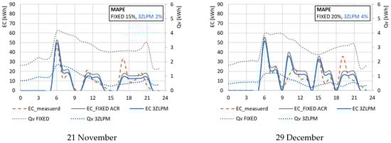
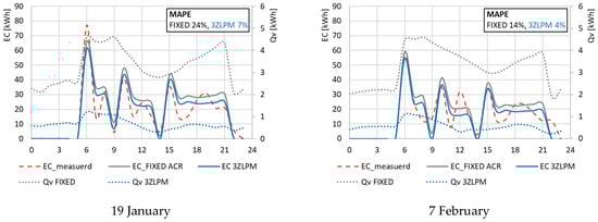
Figure 10.
Hourly energy consumption for space heating with different ACR scenarios and their daily MAPE.
Table 6 reports the monthly MAPE based on aggregated monthly energy consumption during the heating season (November 2022 to February 2023) using available measured consumption data. To provide a more detailed and statistically robust analysis, Table 7 presents the monthly MAPE values calculated from the daily errors, along with the 95% confidence intervals, indicating that 95% of daily prediction errors fell within the specified range.
Table 6.
Monthly MAPE.
Table 7.
Monthly MAPE based on daily energy consumption during the heating season.
Over the entire heating season of 2022–2023, the energy consumption model achieved a 58% improvement with the 3ZLPM compared to using fixed ACR values for the example analyzed building (given in Figure 10). This means that 58% of the total analyzed days improved energy prediction when using building-specific ACR compared to fixed ACR. However, across the 27 buildings analyzed, this improvement was 25% ± 10% (using a 95% confidence interval).
Finally, Figure 11 shows the average building ACR in January for a selected district in Turin with an hourly plot of ACRs for a selected building over a single day. The aim of this map is to demonstrate the applicability of the presented methodology to all residential buildings in a city with a complete geodatabase with building and leakage characteristics.
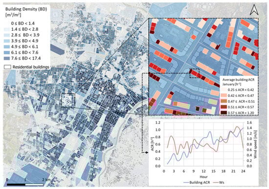
Figure 11.
Average residential building ACR in January in Turin.
4.6. Field of Application of the Methodology
While the methodology presented in this paper provides an efficient approach for estimating ventilation rates in naturally ventilated residential buildings at the urban scale, its applicability is subject to three main limitations. First, the methodology presented accounts for envelope leakage as typically measured by whole-building air-tightness tests, and does not include mechanical ventilation or natural ventilation via open windows. Second, the approach was considered sufficiently accurate for low- to medium-height buildings and has been tested for buildings of up to 16 floors [17]. Finally, the methodology is limited to buildings located within continuous urban canyons, as the wind speed correction method employed in this work relies on this urban configuration.
This 3ZLPM for the ACR calculation was developed for implementation in UBEM, and its level of detail was compared with a detailed building representation. The analysis showed that 3ZLPM was accurate enough for the calculation of whole building ACR for urban-scale applications [17].
5. Conclusions
A comprehensive framework to simulate building ACRs due to infiltration at the urban scale was developed. The methodology integrated aerodynamic parameters influenced by urban morphology into three and four-zone airflow models, demonstrating how local building density and façade orientation impact wind-driven airflow in two contrasting urban environments: a high-density case (New York City) and a medium-density case (Turin). The study further examined the influence of including roof leakage and varying shaft temperatures on hourly ACRs, highlighting the importance of model details in accurately predicting building infiltration. When building-specific, hourly ACRs were implemented in a process-driven UBEM, the simulated space-heating demand showed better agreement with the measured data than simulations using fixed ACR values.
Table 6 and Table 7 confirm that using dynamic, context-based infiltration inputs is essential for reliable energy predictions. Monthly MAPE was reduced by more than half, e.g., in January, it decreased from 21.2% with the fixed ACR baseline to 6.6% when the 3ZLPM approach was applied. At the daily scale, the average prediction errors were reduced from 21.4% to 18.7% in November, representing the smallest improvement, and from 35.4% to 21.1% in December, corresponding to the largest reduction across the 27 analyzed buildings. These results demonstrate that replacing a fixed ACR assumption with realistic, building-specific ventilation rates improves energy predictions, especially in colder months.
However, other factors, such as occupant behavior, were not considered in this analysis and will be addressed in future work. The proposed LPM approach provides a computationally effective framework that can be applied at the urban scale and easily integrated into energy consumption analyses, thereby facilitating large-scale simulations at low computational cost.
Overall, this research demonstrates that combining urban aerodynamic parameters with multizone airflow modeling and integrating the resulting ACR profiles into building energy consumption analyses provides a robust and scalable approach for assessing ventilation loads in urban settings. This enhanced accuracy is vital for urban planners and policymakers seeking to optimize energy usage on neighborhood and city scales.
Supplementary Materials
The following supporting information can be downloaded at: https://www.mdpi.com/article/10.3390/smartcities9020037/s1.
Author Contributions
Conceptualization, G.M. and Y.U.; methodology, G.M. and Y.U.; software, Y.U. and W.S.D.; validation, Y.U. and W.S.D.; formal analysis, Y.U.; investigation, Y.U. and W.S.D.; data curation, Y.U.; writing—original draft preparation, Y.U. and W.S.D.; writing—review and editing, G.M. and W.S.D.; visualization, Y.U.; supervision, C.B., G.M. and W.S.D. All authors have read and agreed to the published version of the manuscript.
Funding
This research received no external funding.
Data Availability Statement
The input data for the ACR simulations with CONTAM for 4 buildings in Turin and New York City are in the Supplementary Materials; other data will be available by the authors on request.
Conflicts of Interest
The authors declare no conflicts of interest.
Abbreviations
The following abbreviations are used in this manuscript:
| ACR | Air Change Rate |
| BD | Building Density |
| CFD | Computational Fluid Dynamics |
| DSM | Digital Surface Model |
| ELA | Effective Leakage Area |
| LPM | Lumped Parameter Model |
| MAPE | Mean Absolute Percentage Error |
| QGIS | Quantum Geographic Information System |
| UBEM | Urban Building Energy Modeling |
| UMEP | Urban Multi-scale Environmental Predictor |
References
- An, L.S.; Alinejad, N.; Jung, S. Experimental study on the influence of terrain complexity on wind pressure characteristics of mid-rise buildings. Eng. Struct. 2024, 321, 118907. [Google Scholar] [CrossRef]
- Javanroodi, K.; Mahdavinejad, M.; Nik, V.M. Impacts of urban morphology on reducing cooling load and increasing ventilation potential in hot-arid climate. Appl. Energy 2018, 231, 714–746. [Google Scholar] [CrossRef]
- Juan, Y.H.; Wen, C.-Y.; Li, Z.; Yang, A.-S. Impacts of urban morphology on improving urban wind energy potential for generic high-rise building arrays. Appl. Energy 2021, 299, 117304. [Google Scholar] [CrossRef]
- Dols, W.S.; Polidoro, B. CONTAM User Guide and Program Documentation Version 3.4; NIST: Gaithersburg, MD, USA, 2020. Available online: https://www.nist.gov/publications/contam-user-guide-and-program-documentation-version-34 (accessed on 18 December 2024).
- Herring, S.J.; Batchelor, S.; Bieringer, P.E.; Lingard, B.; Lorenzetti, D.M.; Parker, S.T.; Rodriguez, L.; Sohn, M.D.; Steinhoff, D.; Wolski, M. Providing pressure inputs to multizone building models. Build. Environ. 2016, 101, 32–44. [Google Scholar] [CrossRef]
- Ng, L.; Zimmerman, S.M.; Good, J.; Toll, B.; Emmerich, S.; Persily, A. Estimating Real-Time Infiltration for Use in Residential Ventilation Control; NIST: Gaithersburg, MD, USA, 2019. Available online: https://www.nist.gov/publications/estimating-real-time-infiltration-use-residential-ventilation-control (accessed on 18 December 2024).
- Santantonio, S.; Mutani, G. QGIS-Based Tools to Evaluate Air Flow Rate by Natural Ventilation in Buildings at Urban Scale. Presented at the BSA Conference 2022: Fifth Conference of IBPSA-Italy, Bolzano, Italy, 29 June–1 July 2022; Volume 5, pp. 331–339. Available online: https://publications.ibpsa.org/conference/paper/?id=bsa2022_9788860461919_42 (accessed on 6 January 2025).
- Sherman, M.H. Superposition in Infiltration Modeling. Indoor Air 1992, 2, 101–114. [Google Scholar] [CrossRef]
- Toparlar, Y.; Blocken, B.; Vos, P.; van Heijst, G.J.F.; Janssen, W.D.; van Hooff, T.; Montazeri, H.; Timmermans, H.J.P. CFD simulation and validation of urban microclimate: A case study for Bergpolder Zuid, Rotterdam. Build. Environ. 2015, 83, 79–90. [Google Scholar] [CrossRef]
- Roberts, B.M.; Allinson, D.; Lomas, K.J. Evaluating methods for estimating whole house air infiltration rates in summer: Implications for overheating and indoor air quality. Int. J. Build. Pathol. Adapt. 2021, 41, 45–72. [Google Scholar] [CrossRef]
- Ku, C.-A.; Tsai, H.-K. Evaluating the Influence of Urban Morphology on Urban Wind Environment Based on Computational Fluid Dynamics Simulation. ISPRS Int. J. Geo-Inf. 2020, 9, 399. [Google Scholar] [CrossRef]
- Palusci, O.; Monti, P.; Cecere, C.; Montazeri, H.; Blocken, B. Impact of morphological parameters on urban ventilation in compact cities: The case of the Tuscolano-Don Bosco district in Rome. Sci. Total Environ. 2022, 807, 150490. [Google Scholar] [CrossRef] [PubMed]
- ASTM E779-19; Standard Test Method for Determining Air Leakage Rate by Fan Pressurization. ASTM: West Conshohocken, PA, USA, 2019. Available online: https://compass.astm.org/document/?contentCode=ASTM%7CE0779-19%7Cen-US&proxycl=https%3A%2F%2Fsecure.astm.org&fromLogin=true (accessed on 10 July 2025).
- Study of Part 3 Building Airtightness—Resources. RDH Building Science. Available online: https://www.rdh.com/resource/study-of-part-3-building-airtightness/ (accessed on 9 December 2024).
- Ramallo-González, A.P.; Eames, M.E.; Coley, D.A. Lumped parameter models for building thermal modelling: An analytic approach to simplifying complex multi-layered constructions. Energy Build. 2013, 60, 174–184. [Google Scholar] [CrossRef]
- Feustel, H.E. COMIS—An international multizone air-flow and contaminant transport model. Energy Build. 1999, 30, 3–18. [Google Scholar] [CrossRef]
- Usta, Y.; Ng, L.; Santantonio, S.; Mutani, G. Lumped-Parameter Models Comparison for Natural Ventilation Analyses in Buildings at Urban Scale. Energies 2025, 18, 2352. [Google Scholar] [CrossRef]
- Mutani, G.; Todeschi, V. An urban energy atlas and engineering model for resilient cities. Int. J. Heat Technol. 2019, 37, 936–947. [Google Scholar] [CrossRef]
- Santamouris, M.; Georgakis, C.; Niachou, A. On the estimation of wind speed in urban canyons for ventilation purposes—Part 2: Using of data driven techniques to calculate the more probable wind speed in urban canyons for low ambient wind speeds. Build. Environ. 2008, 43, 1411–1418. [Google Scholar] [CrossRef]
- Georgakis, C.; Santamouris, M. On the estimation of wind speed in urban canyons for ventilation purposes—Part 1: Coupling between the undisturbed wind speed and the canyon wind. Build. Environ. 2008, 43, 1404–1410. [Google Scholar] [CrossRef]
- Santantonio, S.; Dell’Edera, O.; Moscoloni, C.; Bertani, C.; Bracco, G.; Mutani, G. Wind-driven and buoyancy effects for modeling natural ventilation in buildings at urban scale. Energy Effic. 2024, 17, 95. [Google Scholar] [CrossRef]
- QGIS Web Site. Available online: https://qgis.org/ (accessed on 12 September 2025).
- UNI EN 16798-1:2019; Energy Performance of Buildings—Ventilation for Buildings—Part 1: Indoor Environmental Input Parameters for Design and Assessment of Energy Performance of Buildings Addressing Indoor Air Quality, Thermal Environment, Lighting and Acoustics—Module M1-6. UNI: Milano, Italy, 2019. Available online: https://store.uni.com/en/p/UNI1606278/uni-en-16798-1-2019/UNI1606278 (accessed on 12 December 2025).
- Emmerich, S.J.; Persily, A.K. Analysis of U.S. Commercial Building Envelope Air Leakage Database to Support Sustainable Building Design. Int. J. Vent. 2014, 12, 331–344. [Google Scholar] [CrossRef]
- LBNL Residential. Available online: https://resdb.lbl.gov/ (accessed on 13 May 2025).
- Decree on the National Guidelines for the Energy Certification of Buildings—Policies, Decree of 26 June 2009, Annex A, p. 26. IEA. Available online: https://www.iea.org/policies/19552-decree-on-the-national-guidelines-for-the-energy-certification-of-buildings (accessed on 12 September 2025).
- UNI/TS 11300-1:2014; Prestazioni Energetiche degli Edifici—Parte 1: Determinazione del Fabbisogno di Energia Termica Dell’edificio per la Climatizzazione Estiva ed Invernale. UNI: Milano, Italy, 2014. Available online: https://store.uni.com/uni-ts-11300-1-2014 (accessed on 23 July 2025).
- Dols, W.S. contam-x-jr-ml. Mathworks. Available online: https://www.mathworks.com/matlabcentral/fileexchange/181400-contam-x-jr-ml (accessed on 3 July 2025).
- Usta, Y.; Dols, W.S.; Mutani, G. Urban-Scale Building Air Change Rate Estimation Using Corrected Wind Speeds and Three-Zone Building Modeling. Int. J. Heat Technol. 2025, 43, 1623–1630. [Google Scholar] [CrossRef]
- BDTRE—Geoportale Piemonte. Available online: https://www.geoportale.piemonte.it/visregpigo/?action-type=dwl&url=https:%2F%2Fgeomap.reteunitaria.piemonte.it%2Fws%2Ftaims%2Frp-01%2Ftaimsscaricogp%2Fwms_scaricogp%3Fservice%3DWMS&version=1.3&request=getCapabilities&title=Scarico%20-%20BDTRE%20vettoriale%20(annuale%20-%20struttura%20NC)&layer=scBD3comune (accessed on 6 March 2024).
- Arpa Piemonte: Request Hourly Meteorologic Data. Available online: https://webgis.arpa.piemonte.it/radar/open-scripts/richiesta_dati_hh_2024.php#&ui-state=dialog (accessed on 13 February 2026).
- Gruppo Iren: La Rete di Teleriscaldamento. Available online: https://www.gruppoiren.it/it/i-nostri-servizi/teleriscaldamento/la-nostra-rete.html (accessed on 5 March 2024).
- Building Footprints|NYC Open Data. Available online: https://data.cityofnewyork.us/City-Government/Building-Footprints/5zhs-2jue/about_data (accessed on 14 May 2025).
- Discover GIS Data NY. Available online: https://orthos.dhses.ny.gov/# (accessed on 14 May 2025).
- USGS Lidar Explorer Map. Available online: https://apps.nationalmap.gov/lidar-explorer/#/ (accessed on 7 May 2025).
- EnergyPlus. Available online: https://energyplus.net/weather-region/north_and_central_america_wmo_region_4/USA/NY (accessed on 3 July 2025).


Disclaimer/Publisher’s Note: The statements, opinions and data contained in all publications are solely those of the individual author(s) and contributor(s) and not of MDPI and/or the editor(s). MDPI and/or the editor(s) disclaim responsibility for any injury to people or property resulting from any ideas, methods, instructions or products referred to in the content. |
© 2026 by the authors. Licensee MDPI, Basel, Switzerland. This article is an open access article distributed under the terms and conditions of the Creative Commons Attribution (CC BY) license.