


Abstract
Researchers have described the manner in which the low-level information from images varies with regard to orientation distribution, referred to as the level of anisotropy in an image. Prior work has described deviations from typical real-world (nature, suburban, urban) images in the content of various categories of digital images, including games, social media, and others. The present work extends prior findings by bandpass filtering images across nine categories, analyzing orientation content within each bandpass range and comparing anisotropy across spatial frequency. Anisotropy in this analysis was found to increase with spatial frequency; relatively isotropic orientation information was present in the low bandpass range across all image categories, while medium and high bandpass images show a pattern of increasing anisotropy in a category-dependent manner. In particular, deviations from the distribution defined by nature images characterize multiple categories of digital images; this finding is discussed in terms of potential implications for visual system plasticity and the potential for such changes to impact multiple facets of perception. Potential impacts of this finding on training sets for machine learning tools are also discussed.
1. Introduction
Field [1] argued that an understanding of the neural properties of the human visual system must be informed by analysis of the properties of the visual world that gave rise to the system. This assertion, that the current state of the visual system is driven by the nature of inputs from the visual world and is thus susceptible to change, serves as a basis for our current understanding of multiple aspects of the visual system, in that a close correlation between local statistics of contours in the visual world and perceptual processes has been well-demonstrated [2,3,4]. Bao and Engel [5] and others [6,7,8] have established the effects of exposure on various aspects of the visual world on visual system responses, focusing in particular on the plasticity of the visual system. This malleability is notably demonstrated in orientation sensitivity [9,10,11] and in spatial frequency [12,13,14], two dimensions of visual information contained in images that are clearly understood to be directly represented in the early visual system [15,16,17,18].
One such change in orientation sensitivity as a result of this malleability is known as the oblique effect, in which the human visual system adapts to increase sensitivity to the most prominently represented orientations in the environment [9,10,19,20]. Differences between the natural and carpentered environment and, more generally, across cultures [21] clearly influence the level and even the direction of the effect. Analyses of the level of anisotropy, or the level of oblique representation compared to canonical, in particular environments [11,22,23] confirm that carpentered environments contain an increased amount of horizontal and vertical contours compared to oblique, whereas natural environments are less anisotropic [19,22,24,25,26]. These differences across orientation and environment suggest that the specifics of the visual input characteristic of a particular environment exert an outsized influence on sensitivity in the exposed perceiver. Even short exposures to stimuli with an altered orientation profile result in detectable changes in the response profile of orientation sensitivity [10]. Most pertinent to this discussion, Duggan and Gerhardstein [22] analyzed digital media images and found that multiple digital media contexts show a profile of increased anisotropy relative to nature, suburban, and even urban environments. The current investigation is intended to expand this finding to describe changes in orientation as a function of spatial frequency, and to discuss implications of this relationship.
Similar to orientation, the visual cortex displays tuning to specific spatial frequencies [27]. This tuning consists of channels in which neurons are maximally sensitive to a small range of spatial frequencies. While there are multiple individual spatial frequency channels [12,28], channels can be categorized by splitting them into low spatial frequency and high spatial frequency bands [27,29,30,31]. Low spatial frequency bands include broad, smooth variations in intensity across an image, referred to as the global structure of a scene, whereas high spatial frequency bands include the fine, sharp details of an image, referred to as the local structure [1,27]. Gao et al. [32] and Flevaris et al. [33] have shown that attention to local features of an image enhances high spatial frequency processing, demonstrating the flexibility of spatial frequency processing. Alongside this, prolonged exposure to specific frequencies influences the visual system’s sensitivity to specific bands through adaptation, decreasing the sensitivity of neurons sensitive to that particular frequency and, in turn, increasing the detection threshold [34,35].
Similar to orientation, images have been shown to contain differing levels of contour as a function of spatial frequency. This is the well-known “1/f” function in that contour content, as measured by amplitude spectra, declines in this manner as spatial frequency increases [36,37]. Field and Brady [38], as well as many others, note that the statistics of natural scenes appear to drive an organization of the cortex along the dimension of spatial frequency as well as orientation, and that there is a whitening mechanism that causes responses to increase to compensate for the 1/f decline, particularly as recently experienced anisotropy varies [39]. It is the case, however, that not all images show exactly the same rate of drop, leading to an altered function; 1/fɑ [39,40,41], with the alpha parameter being specific to scene type. The variations in the function reveal certain image characteristics. According to Nguyen and Spehar, the ɑ-value of images is indicative of visual preference, with an ɑ ≈ 1–1.25 being the most preferred. Spatial frequency adaptation also appears to shift this preference toward the adapted ɑ-value, suggesting the parameter’s importance in visual perception [40].
Different environments contain varying proportions of spatial frequency information, as is the case with orientation. Urban and indoor environments, for example, are over-represented by high spatial frequencies, while natural environments contain a more even distribution of high spatial frequencies and low spatial frequencies [23]. This phenomenon appears to be similar to the oblique effect with contours, revealing disparities in spatial frequency content between natural and carpentered environments. The visual system appears to adapt to spatial frequency distributions in the viewed environment alongside orientation distributions [34,41], suggesting potential behavioral changes caused by over- or under-representation of specific spatial frequency bands. Spatial frequency is critical for visual perception, playing a role in facial recognition [42], size encoding [43], and arguably in overall object recognition [44]. Spatial frequency adaptations therefore have the potential to impact visual perception and behaviors driven by perception. Hipp et al. [10] found that a single long exposure to canonical lines exacerbates the oblique effect in orientation. As orientation and spatial frequency are tied together in the perception and integration of contours, it may be that spatial frequency adaptation stemming from exposure to an environment presenting a deviation in the statistical distribution of spatial frequencies also causes a shift in visual perception. It should be noted, however, that work in this area to date has typically used predominantly natural images [36,45], and thus one motivation for the current work is to extend this type of analysis into the domain of digital media, which is now a major source of visual input for children across a swath of development as well as a strong influence on global culture and exposure as a whole.
Differences Between Digital Media and Natural Images
Duggan and Gerhardstein [22] found that multiple types of digital media contain large degrees of anisotropy compared to natural, suburban, and urban environments, in good agreement with prior work examining the properties of visual images [36,46], with potential implications for chronic media exposure. Understanding such differences has become increasingly important, as individuals are spending more and more time on digital devices. Viazcaino et al. [47] reported that the majority of adults in 2019 spent a significant amount of time using various devices. Various reports [48,49] indicated that over 83% of adults and 84% of 18–29-year-olds use at least one social media platform daily. Indeed, an advisory report by the Surgeon General [50] indicated that social media use in adolescents has reached epidemic levels. CommonSense Media [51] found that children 0–2 years old used media for ~50 min per day, 2–4 used 2.5 h per day, and 5–8 used media for over three hours per day. Estimates for adults across multiple ages are also quite high [52,53].
Thus, understanding how this type of digital media differs from the natural world is likely to inform research on the impact of high levels of media exposure on children’s development as well as visual perception more broadly. Multiple findings [54,55,56,57,58] have shown that visual perception proceeds along a ‘coarse-to-fine’ progression, with lower spatial-frequency magnocellular pathway information preceding information flowing to the parvocellular pathway at higher spatial frequencies [59]. Note that this finding has impacted multiple machine learning approaches as well [60,61,62], with one finding [63] showing that a model supplied first with coarse and then across training with more fine-grained images outperforms the same model when trained only with complete images. The authors concluded that the progression in visual acuity seen in human development may convey advantages to learning of object representations.
Other work has applied an emerging approach in machine learning that uses multi-scale feature extraction to improve performance and reduce model complexity and computational demands [64,65,66]. Overall, these studies emphasize that an increased understanding of how information within images varies across spatial scales in many different contexts is important. These observations further motivate the present analysis; if digital media offer a different set of low-level statistics overall, and in particular present different levels of orientation information at different spatial frequencies relative to natural images, then development and CNN training with digital images may be expected to generalize poorly to the natural world and the reverse.
With regard to human perception in particular, if different spatial frequency bands carry differing distributions of orientation information, then deviations between the natural world and digital content would have implications with regard to the information available for development and perception. A child who is exposed to a high degree of digital media across development might, if there is a substantially different signal in terms of orientation and spatial frequency, acquire a clearly deviating level of information supplied to the parvocellular system as compared to the magnocellular system, resulting in the child’s ‘internal model’ differing from the real world in which they live, and with implications for the mature system. As the above discussion notes, such differences may affect model performance as well as human perception [67], demonstrating a need for a more detailed and nuanced understanding of the interaction of image (signal) information at multiple levels of spatial frequency and orientation in multiple contexts such as digital media.
These findings, in combination with evidence suggesting that the environment has a major impact on visual system sensitivity [5,68,69], support an argument that sufficiently increased exposure to digital media may be enough to alter visual perception in children and adolescents, as well as impacting the performance of classification models as a function of the type of image used in the training set. Despite these points, a systematic examination of how orientation and spatial frequency information interact is difficult to find. Several groups [70,71,72] have reported that orientation content is not invariant across spatial frequency, but these authors presented only analyses of natural images, further motivating an investigation of differences between digital media and natural images in this regard. Duggan and Gerhardstein [22] in particular did not include the factor of spatial frequency when examining content-based differences in orientation anisotropy. As contour integration (among other processes) is impacted by both orientation and spatial frequency [73,74,75], elucidating these differences is an important initial step in understanding the impact of extensive exposure to highly anisotropic or otherwise altered digital media on perception and cognition. Thus, the goal of the current investigation is to analyze digital content both in terms of orientation and spatial frequency in comparison to natural and other non-digital images, including suburban and urban content. In this analysis, the overall spatial frequency content of digital media and natural, suburban, and urban scenes were compared alongside the orientation content within specific spatial frequency bandwidths (low, medium, and high). This was done using Fourier analysis (Equation (2)) to reveal spatial frequency and orientation disparities within digital media. This approach clarifies the contribution of different spatial frequencies to orientation disparities and, by doing so, reveals the potential influence of different pathways in the visual system on orientation bias as a function of image category. It is expected that digital media contains comparable amounts of low spatial frequency information compared to real-life scenes with less high spatial frequency content. This disparity is expected to be further exacerbated in the analysis of orientation content within specific spatial frequency bands, as it is anticipated that digital media exhibits high degrees of orientation anisotropy within high spatial frequency bandwidths.
2. Materials and Methods
In order to assess differences in image content by category across orientation and spatial frequency, images from nine different categories of digital media and ‘real world’ sceneries were collected and sorted into: Nature scenes, suburban scenes, urban scenes, children’s cartoons, social media websites, news and professional websites, nature-based video games, urban-based video games, and pixel-based video games. The choice of categories followed Duggan and Gerhardstein [22]. These images were captured from publicly available videos in full screen by taking screenshots every 5–10 s. Images were taken at full screen to maximize the size of the picture while avoiding unnecessary elements of the video platform and computer graphical user interface to maintain image uniformity. No additional compression or preprocessing was added. Images of real-world scenes were taken from publicly available videos on YouTube and separated into three different categories (multiple videos per category), with the aim of representing different locations, using different creators, and with variability somewhat similar to that of the digital sources:
- Nature scenes:
- ○
- Include images taken in various biomes (mountains, canyon, forest and woods/open parkland);
- ○
- Contain only natural elements; human-made structures explicitly excluded.
- Suburban scenes:
- ○
- Include images taken in various US suburban neighborhoods;
- ○
- Contain a mix of natural and human-made elements with occasional people.
- Urban scenes:
- ○
- Include images taken in downtown Manhattan, Rome, San Francisco and Seattle;
- ○
- Contain mainly human-made structures and human activity with sparse natural elements.
Images from cartoons were captured from publicly available videos of various children’s shows. Social media images were captured from various platforms from a single person’s account, while other professional website images were captured from public websites or publicly available videos. These categories were described as follows:
- Children’s cartoons:
- ○
- Animated television shows marketed towards young children (2–5 years);
- ○
- Most present a simplistic 2- or 3-dimensional animation.
- Social media websites:
- ○
- Websites used to share media, including images, statements, and videos.
- News and other professional websites:
- ○
- Websites used to gather current information or used in a professional setting;
- ○
- Includes the e-commerce business Amazon due to its popularity.
Video games were separated into three categories based on video game content:
- Nature-based games:
- ○
- Video games with content intended to mimic nature;
- ○
- May contain constructed aspects such as houses.
- Urban-based games:
- ○
- Video games taking place mostly in urban settings;
- ○
- Little to no natural elements.
- Pixel-based video games
- ○
- Exhibit a “pixel-based” graphical art style; highly granular (e.g., Minecraft);
- ○
- Created imagery using pixel art to mimic video games of the 1980s, 1990s, and early 2000s.
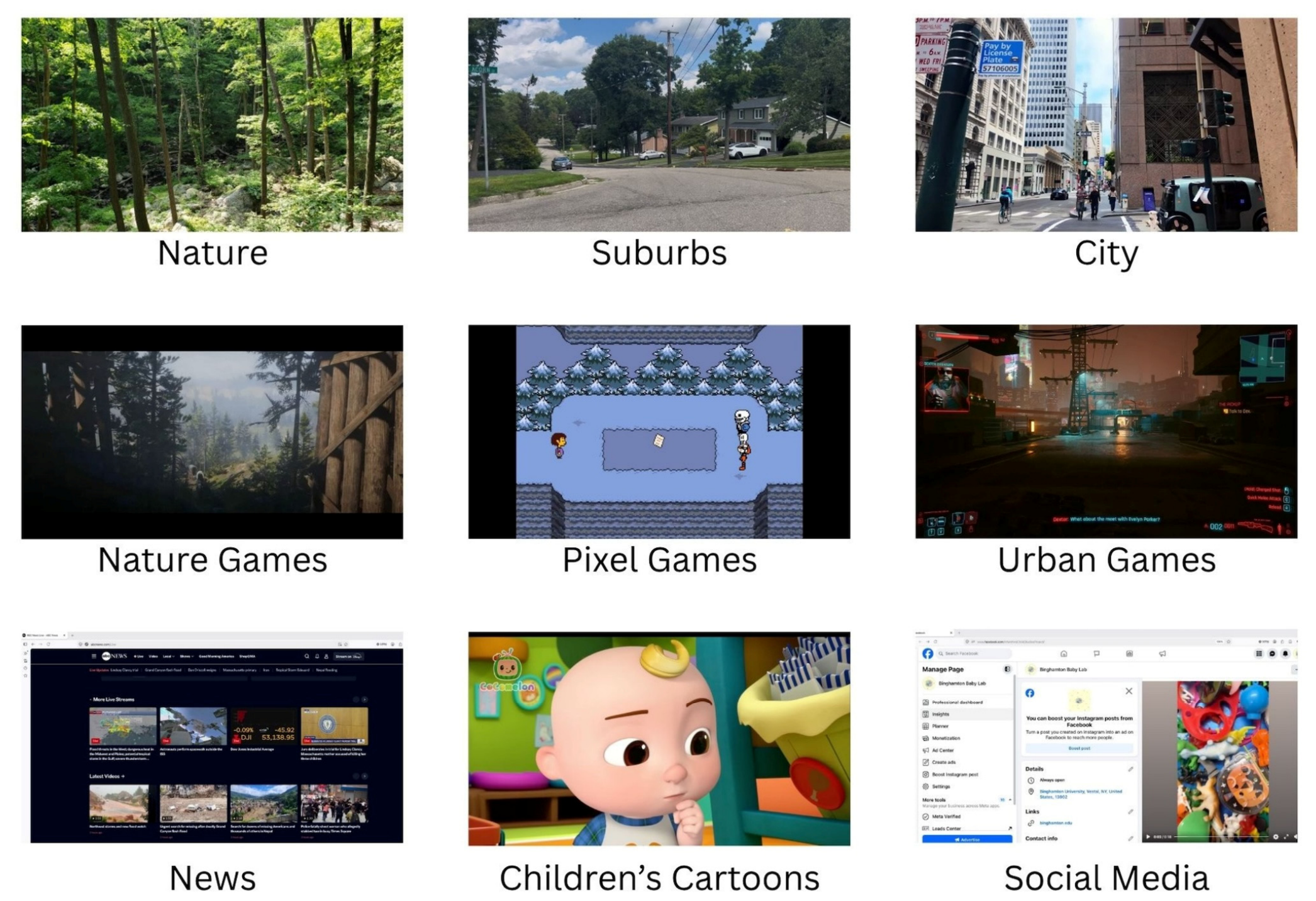
Video games were chosen and sorted based on judgment of their fitness to the category by the authors. All images were captured at 1920 × 1080p, and at least 300 images were collected from each source (mean of 3000 per category, 18,797 images in total). No source contributed more than 700 images. See Table 1 for a listing of image counts, and Figure 1 for examples of images from each category.
Table 1.
Listing of image categories, specific category entries, and number of images per entry.
2.1. Standardization of Images
Prior to analysis, the collected images were standardized as follows: Images were passed through a grayscale filter [using MATLAB’s version R2023.b rgb2gray function; Equation (1)] and cropped to an 800 × 800 pixel circle following the approach of Schweinhart and Essock [11] to eliminate any orientation-specific border effects.
R, G, and B components of color pixels are weighted to retain only luminance (Matlab rgb2gray [76]):
gray = 0.2989360212 × R + 0.5870430744 × G + 0.1140209042 × B
Figure 1.
Examples of each image category. (Top row) includes real world scenes, (middle row) includes video game categories, and (bottom row) includes a news website, children’s cartoon, and social media. (Top-left) Image by D. Hipp. (Top-middle) Image by author (PG). (Top-right) World Explorer 4K [77]. (Mid-Left) Red Dead Redemption 2 by Rockstar Games. (Middle) Undertale by Toby Fox. (Mid-right) Cyberpunk 2077 by CD Projekt. (Lower-left) Image from ABC NEWS CHANNEL (A division of AMAZON MEDIA LLC). (Lower-mid) Cocomelon by Moonbug Entertainment. (Lower-right) Facebook image (by author PG).
2.2. Analysis Plan: Image Analysis—Spatial Frequency
The overall analysis performed was split into three parts. First, the total spatial frequency of chosen images was obtained using a fast Fourier transform [78] (Equation (2)). Next, images were parsed into three spatial frequency categories (low, medium, and high as described below) by passing them through bandpass filters using the same FFT. Finally, contour information was extracted by taking a horizontal and vertical FFT summed across all rows or columns, rotating the image three degrees, and repeating until the image was rotated 90°. This approach enabled a comparison of orientation information across all spatial frequencies and between image categories. The visual information thus extracted reflects the extent of horizontal, vertical, and oblique contours within each spatial frequency range.
where Wn = e(−2πi)/n
For an input vector X of length n;
Wn is one of the roots of unity for the equation;
k = output index (the frequency bin).
2.3. Image Analysis—Total Spatial Frequency
Frequency information from each image was collected and summed within each image using the FFT function in Matlab (Equation (2)) and subsequently averaged across all images in each category. The maximum sampling rate for analyzing frequency information was driven by the Nyquist Sampling Theorem. The sampling rate, based on an 800 × 800 pixel image, was 400 samples/image. The highest spatial frequency possible within each image was 400 cycles/image, or 0.5 cycles/pixel. To ensure accurate representation of spatial frequencies within each image, a sampling rate of 400 samples/image was used to match the highest possible spatial frequency of each image. The average magnitude of the FFT within each category was plotted against the sampling rate calculated to obtain the frequency representation plots. All frequency graphs were plotted on a log–log graph.
2.4. Image Analysis—Bandpass Filters
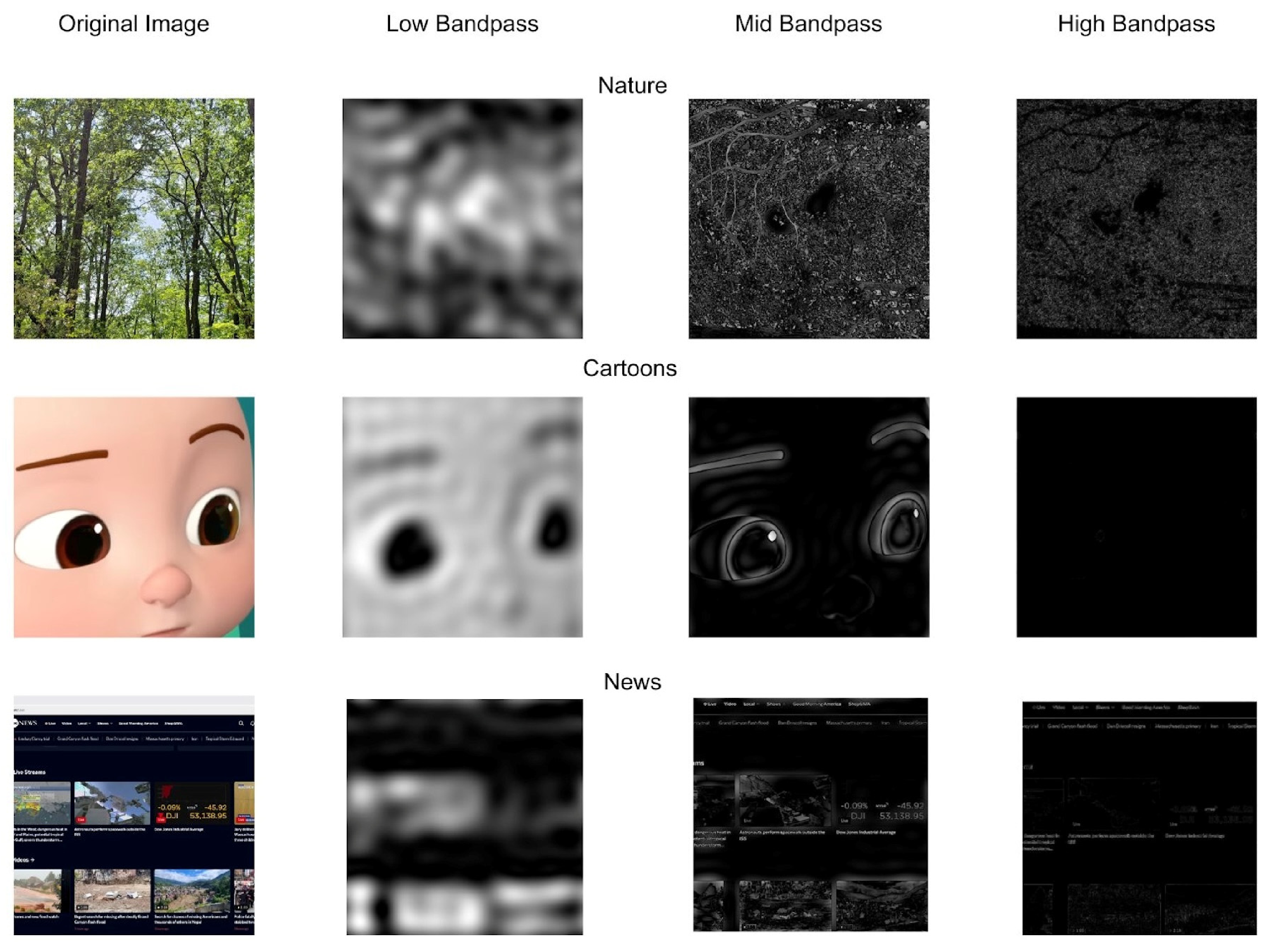
After transformation, three bandpass filters were applied to each image to obtain the spatial frequency information contained within different frequency bands. These filters consisted of a low-bandpass filter (0–0.01 cycles/pixel or 0–8 cycles/image), a mid-bandpass filter (0.01–0.2 cycles/pixel or 8–160 cycles/image), and a high-bandpass filter (0.2–0.5 cycles/pixel or 160–400 cycles/image). These ranges correspond (roughly) to 0–2.75 deg., 2.7–7.25 deg., and 7.25–18 degrees visual angle at an assumed distance of 60 cm. These filters were chosen based on the amount of perceived information present in each image, specifically within nature images: Bandpass filters were applied to nature images, and the subsequent filtered images were observed by multiple observers, including the authors, to perceptually (subjectively) determine appropriate filter ranges. Filter ranges were chosen based on the amount of visible information present in each image, and the ability of researchers to discern at least the category of the original image (note that the same bandpass ranges were used for all categories, however). The choices of cutoff points agree well with information regarding the visual system’s response to different spatial frequencies [38] and the overall range of contrast sensitivity across spatial frequency. The mid-range brackets the point of highest spatial frequency sensitivity (~4 cpd) in human vision [16,79], but see [80] for discussion regarding differences in everyday vision. The low–mid cutoff in this analysis falls near the point at which processing may shift from the magnocellular to the parvocellular system [81] or ‘transient’ to ‘sustained’ [82], although certainly the literature does not support the idea of a strict “junction” between these two pathways [83]. The high bandpass thus defined encompasses a range of frequencies within the normal resolvable acuity range, but past peak sensitivity.
The goal of the chosen filters was to split the amount of visual information roughly equally between the three bandpass ranges while maintaining the ability of observers to match the filtered image to the original image to some degree. As can be seen in Figure 2, this was not always achieved for every image. Application of a filter retained only the visual information encoded within the spatial frequency range of that filter. This produced three distinct images with visual information associated with (only) low, medium, or high spatial frequencies. An inverse FFT was applied (IFFT2 function [78]) to each bandpass image to re-create the filtered image displaying contour information specific to spatial frequencies within the desired bandpass range (see Figure 2).
Figure 2.
Example of gray-scaled and bandpass-filtered images in comparison with the original image before image preprocessing. Examples of a nature image ((row 1) image by D. Hipp), children’s cartoon ((row 2) image from cartoon ‘Cocomelon’ by Moonbug Entertainment), and a media website ((row 3) image from ABC NEWS CHANNEL—A division of AMAZON MEDIA LLC).
2.5. Image Analysis—Contour Orientation Information
The vertical and horizontal content from each image was sampled by applying the FFT2 function in Matlab [78] (see Equation (2)). The image was then rotated 3° and sampled again to obtain the contour content at additional angles iteratively until the image had been rotated 90° (see Figure 3).
Figure 3.
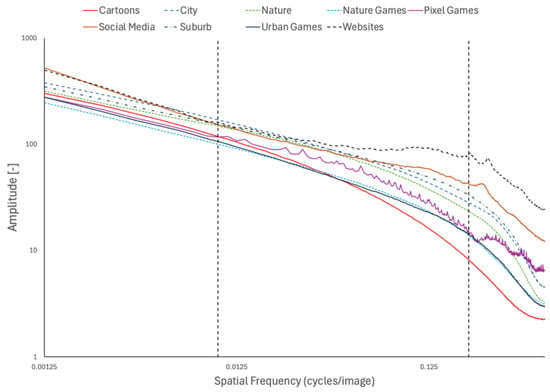
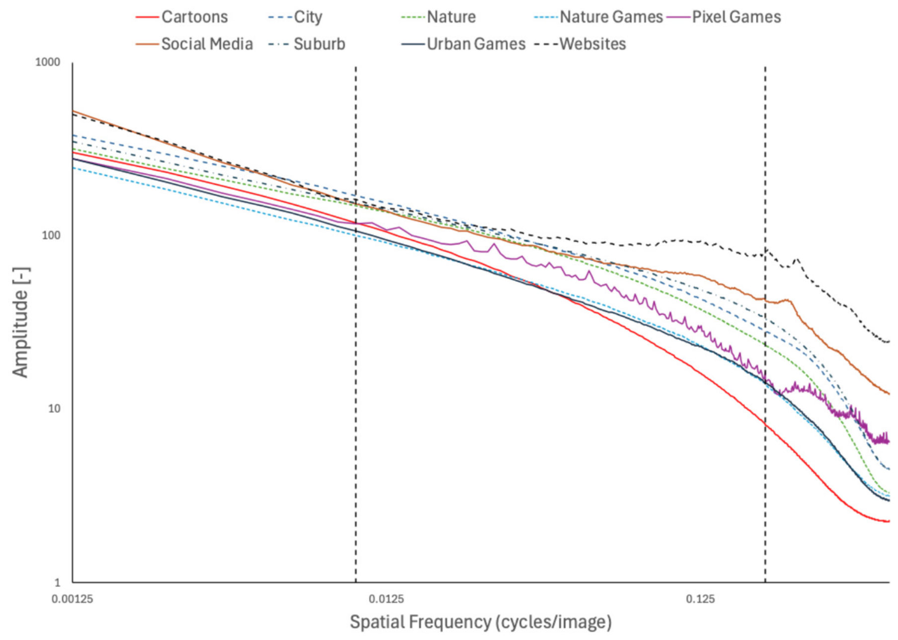
The amplitude of each category as a function of spatial frequency. The plot is split up into three separate areas: the low bandpass range (left area, 0–0.01 cycles/pixel), the middle bandpass range (middle, 0.01–0.2 cycles/pixel), and the high bandpass range (right, 0.2–0.5 cycles/pixel). Note that amplitude is uniformly high in the low spatial frequency range, while deviation increases in the middle, with substantial deviation clearly visible in the higher spatial frequencies. The natural images are relatively tightly clustered in a mid-range across the middle and high spatial frequencies.
3. Results
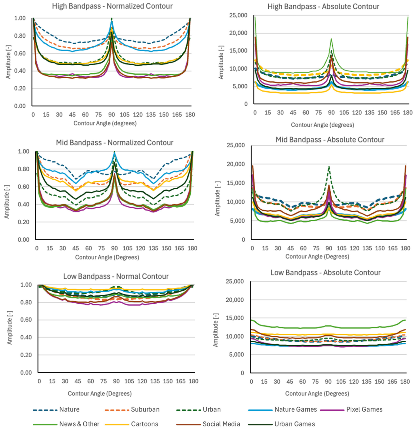
The results of the FFT were imported into R [84] and analyzed as appropriate for the different questions. As in Duggan and Gerhardstein [22], mean amplitude was normalized within individual images to correct for mean differences in amplitude across individual images and across categories. Initially, contour was analyzed using factors of spatial frequency (low, medium and high), contour (horizontal, vertical, and oblique), and general category of image (nine levels). Oblique for the analysis was defined as 45 degrees. See Figure 4 for a depiction of the outcome of the filtering as a function of category, orientation and spatial frequency.
Figure 4.
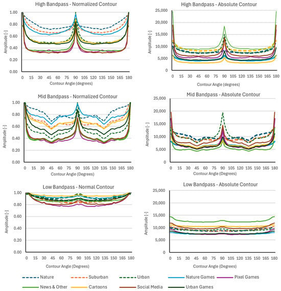
The interaction between spatial frequency and anisotropy profiles can be seen across the six panels. The left column depicts the normalized orientation anisotropy, while the right column depicts absolute anisotropy, to allow for comparison of overall level across the three ranges of spatial frequency. Orientation anisotropy (within each panel) shows a notable change across spatial frequency, increasing non-uniformly as spatial frequency increases. Nature images, suburban images, and nature game images are clearly clustered as the most isotropic in the high bandpass images.
The data were analyzed using a hierarchical (mixed-effects) model (glmer; [84]). The dependent measure was anisotropy magnitude, referred to as amplitude, as returned by the FFT, with fixed factors of spatial frequency (low, mid, and high), orientation (0, 45, and 90) and category, with orientation nested within spatial frequency. To account for the fact that individual images were drawn from a common video within each of the categories, both video and image were included as random factors: Each image received a Video ID and an Image ID that was unique across the entire data set, but identified the nine images resulting from the cross of spatial frequency and orientation as having a common source image (all nine shared the same Image ID). Video ID indicates the existence of a common origin for all images from that video, which allows the mode to account for correlations between these images by treating this as a random factor. Figure 3 depicts the data by spatial frequency, collapsed across orientation.
To investigate the effects of video type within each category, intra-class correlations (ICC) were conducted across all images for each category separately. All but one category (Pixel Games) showed an ICC < 0.11, with five of the nine less than 0.06. The pixel games category showed an ICC of 0.20, indicating that within-video similarity of images was slightly elevated, relative to between-video similarity. This, however, is exactly what we would expect in this type of game and speaks to the differences in what an observer experiences when interacting with this type of digital content in comparison to, for example, nature or suburban content. These correlations suggest that images from within a particular video are about as similar as images from different videos (within a category). An overall ICC analysis resulted in an ‘adjusted’ (after controlling for all fixed factors) of 0.36, with VideoID at 0.16, and ImageID at 0.20, revealing relatively low correlation due to the common source of multiple images in the data set.
The model resulted in a clear indication of significant effects for all factors (Category, Spatial Frequency, and Orientation) and all interactions. F statistics from this model, generated by the emmeans package in R 4.5.2 [84], are reported in Table 2. The df for the denominator in all cases for this model is “Inf” due to the large number of total observations (170,055). While this is legitimate in the case of Spatial Frequency and Orientation, when Category is involved, this may cause an issue, as Category contains 39 videos and the images within each are correlated to some extent. As a result, the df is likely an overestimate, and the model’s reported statistics for all terms involving Category may overestimate its true impact [85,86,87]. To confirm that the overall model is not exaggerating the effect of Category, a second analysis was conducted in which the data were collapsed across individual images (also reported in Table 2). In summary, as can be seen in Table 2, all main effects and all interactions are reliable, whether the full hierarchical model or the limited aggregate model is considered.
Table 2.
F-test results from the analysis of Category, Spatial frequency level, and Orientation. The left analysis takes into account both the random factors of Video and of Image, while the right is collapsed across Image to present a more conservative analysis of the effects of Category. Note that all p-values for every main effect and interaction in the full model are p << 0.0001.
While the initial overall analysis confirms that the effects are reliable, specific contrasts are needed to address questions pertinent to the investigation. First, a set of three contrasts between spatial frequency level and category were conducted at each level of orientation (H, V, and O). Because Category was involved in these contrasts, while noting that the full model indicated clearly significant interactions for all three levels, the aggregate model output is reported (all main effects were significant, but as they are not informative here, they have been omitted). The aggregate model produced significant category × spatial frequency interactions at horizontal; F(16, 240) = 7.36, p < 0.0001 and vertical; F(16, 240) = 5.16, p < 0.0001. At the level of ‘oblique’, however, the aggregate model interaction was not reliable; F(16, 240) = 1.41, p = 0.13, meaning that the pattern of Category differences did not change across Spatial Frequency for this orientation.
This was true despite the fact that the SD within category for the ‘oblique’ level was lower than that for the other two levels, suggesting that the effects are driven by pattern differences in the ‘horizontal’ and ‘vertical’ levels rather than a higher level of variability in the ‘oblique’ level. See Figure 4 for a depiction of the data from each level of each factor.
Next, contrasts in the reverse situation were applied, holding spatial frequency constant at each level (Low, Mid, High) and analyzing orientation and category in each isolated context. Again, the aggregate model output is reported; the (unreported) full model showed reliable effects in all cases (but the F-value for ‘Low’ was considerably lower). In the aggregate model, high spatial frequency resulted in F(16, 240) = 8.77, p < 0.0001 and Mid resulted in F(16, 240) = 7.03, p << 0.0001. Low spatial frequency, however, showed a non-significant result; F(16, 240) < 1. It could be argued that the use of the aggregate model here is too conservative, but we prefer to use this approach because the full model may be using more degrees of freedom than the model can justify when Category is involved [88].
Analysis of α Values for Slopes
Figure 3 and Figure 4 illustrate spatial frequency and orientation differences between image categories. Figure 3 highlights disparities in overall spatial frequency, especially in high spatial frequencies. The slopes of the spatial frequency plots, modeled as a 1/fα function [36,39], were used to determine α-values within low, mid, and high bandpass ranges (see Equation (3)). These values indicate how quickly information content decreases as spatial frequency increases, showing where most spatial frequency loss occurs in different image types. In practice, alpha values were calculated using the lm function [84] to generate a linear fit in R across the log of amplitude and frequency for the full bandpass range. This calculation assumed linearity in the spatial frequency plot, although Figure 3 shows that this assumption is of limited validity.
for (f1, A1) and (f2, A2) defined by frequency (f) and amplitude (A).
α = −log(A2/A1)/log(f2/f1)
Table 3 presents these values, where a larger α-value signifies a steeper decline in spatial frequency information. As expected, the highest α-values appeared in the high spatial frequency range, except for the children’s cartoon ‘Cocomelon’, which showed the largest α-value in the mid-bandpass (apparently because Cocomelon images contain essentially no high spatial frequency contours). Most categories show high values in the high spatial frequency range, confirming that the drop-off in content is increasing in this range. Nature-based and urban-based video games were extremely close to their natural world counterparts. Generally speaking, natural world images reflected higher average values in the high-frequency range in comparison to digital media, with some exceptions as can be seen in Table 3.
Table 3.
Category geometric means of the α-values for the slopes of functions for different content in the image analysis, including the specific α-value within the low, middle, and high bandpass.
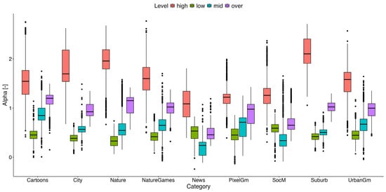
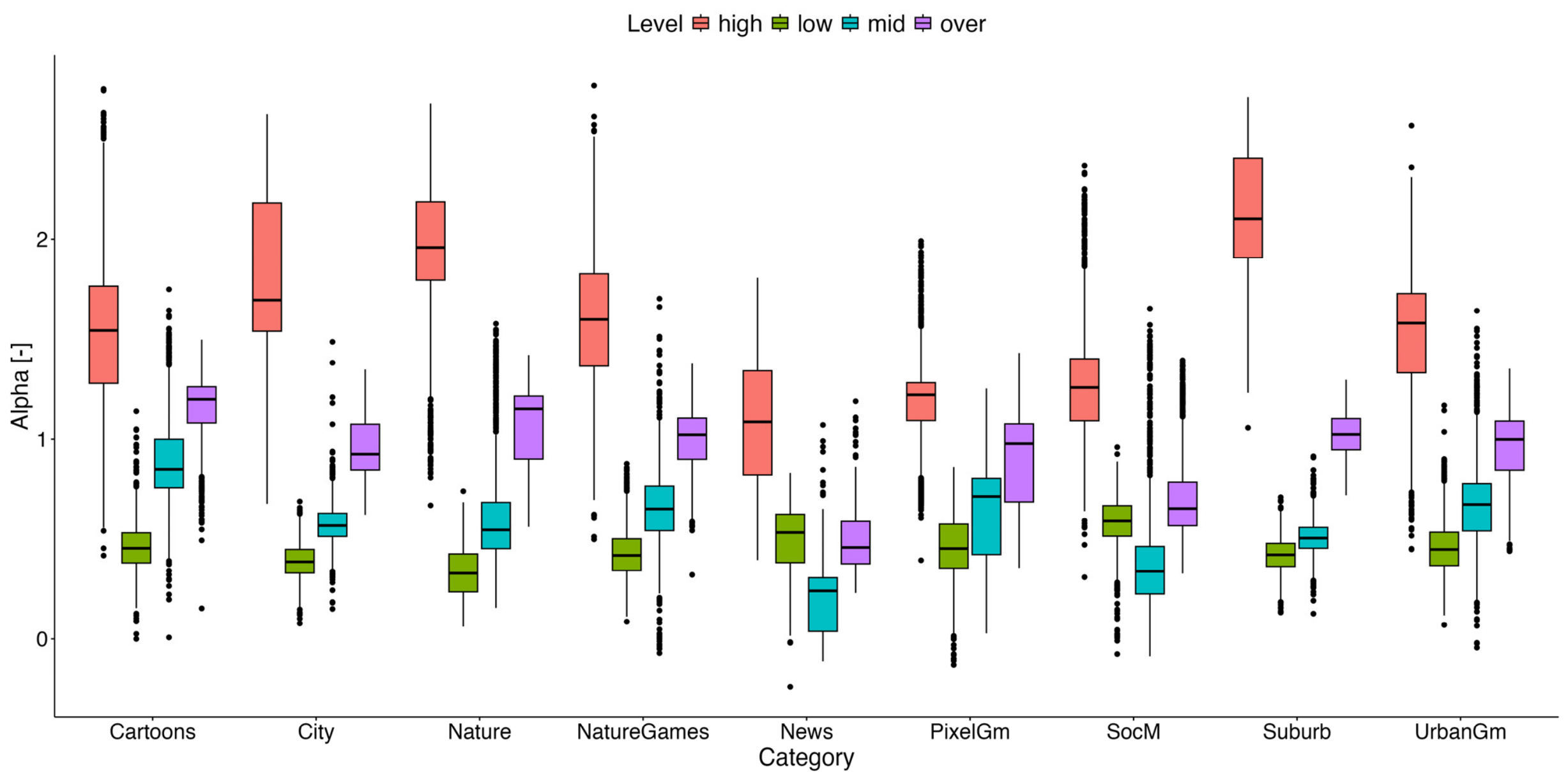
Pixel-based video games had the lowest overall α-value and were lowest across the spatial frequency bands, likely due to significant variability between games. Social media and news websites also had lower α-values, lower than all real-world scenes, meaning that they contained an inordinately high amount of high spatial frequency contour, and showed a slowed 1/f decline in general. The α-value of each individual image at each bandpass level and overall was calculated and used to form the boxplot in Figure 5. There is significant variation between images within categories, specifically at high spatial frequencies, but overall, a trend toward higher alpha values is seen in the high spatial frequency range for most, if not all, categories. Negative α-values were found within specific images, again suggesting significant variation within categories. This occurred in particular when looking at the high bandpass α-values within pixel-based video games, cartoons, news, and other websites. The α-values within mid- and low-bandpass ranges show much less variation compared to high bandpass, revealing disparities within categories’ high spatial frequency representation.
Figure 5.
Boxplot comparing individual image α-values sorted by category (cityscape, nature, suburban, nature-based, urban-based, pixel-based, cartoon, social media, and news and other) and bandpass filtering (low, mid-level, high, and overall).
4. Discussion
Analysis of over 18,000 images across nine categories broken down by both spatial frequency and orientation demonstrated that anisotropy is non-uniform across spatial frequency. Overall, amplitude within images decreased as spatial frequency increased. This is predicted by prior work showing the referenced 1/f function for spatial frequency [1,38,40,89,90]. A relationship between orientation and spatial frequency was also seen, however, reflecting the observation that low frequencies are relatively isotropic, with anisotropy increasing substantially in the mid- and high-frequency ranges. This is particularly interesting in the context of the image categories chosen for analysis; while digital images overall show the same 1/f pattern as ‘real world’ images, the alpha values of their 1/f slope functions reflect significant departures from the pattern for non-digital images, and in particular deviate from the function that characterizes natural images. This reflects the complex interaction between orientation and spatial frequency as a function of category and is in large part due to increases in the absolute amplitude at horizontal and vertical orientations in mid- and high-level spatial frequencies for most of the digital image categories; levels are similar across most of the oblique orientation range in all three spatial frequency bands.
News content was found to be the only digital category containing significantly higher amplitude overall in comparison to natural images (in any of the three categories) in the high spatial frequency band in particular; this can be seen both in Figure 3 and in Table 3. All other categories of digital media also appear to deviate from the function describing natural (and indeed suburban) images as well, with a combination of differences across mid- and high-level spatial frequencies. This has implications for perception, as this type of deviation from the statistical distribution of amplitude spectra across spatial frequencies has been shown to elicit negative ratings and reactions in observers [89]. For an informative review see [90,91,92,93]. Le et al. [93] in particular note that viewing specific types of scenes (in their case, urban scenes) elicits measurable discomfort, relative to viewing nature scenes, and the current findings suggest that at least some types of digital material may drive similar shifts in affective perception.
Whether this type of finding persists in individuals with extensive exposure to the altered slope functions that characterize different types of digital media is unknown, but appears to be an important question [10]. Nguyen et al. [40] have shown that extended exposure to images of specific spatial frequency alters preference toward the adapted spatial frequency, and local orientation statistics underlying scenes have been shown to contain substantial information for vision [3,4,94], so the idea that affectively pleasing and negative images can be differentiated on the basis of spatial frequency or other low-level information is supported by multiple prior studies [39,91,93,95]. Thus, it is possible that the current generation of digital natives is altering both their visual perception and their affective interpretation of that perception [96,97,98] through their consumption of digital content.
Ogawa and Motoyoshi [89] note that this change in affective perception is not limited to deviations across spatial frequency, but is also observed when the level of anisotropy in an image changes. They tested images with deviations from identified statistical distributions in spatial frequency and orientation and reported that observers rated these deviating images as less pleasant (or unpleasant) in both cases. Factors of orientation and spatial frequency interacted in their results, with the implication that the relationship seen in the current analysis of images may well lead to an interaction in the perceptual impact of spatial frequency and anisotropy.
Returning to a point from the introduction, multiple researchers testing scene and object recognition [54,55,57,99] have found that the visual system processes low spatial frequencies rapidly and with relatively high fidelity [94,100], demonstrating the primary importance of this range of frequencies for recognition. The ‘coarse-to-fine’ argument [55,94] has attracted substantial attention in this literature [101,102,103]. It should be noted that high spatial frequencies are certainly important to facial recognition [94,100], and that certain specific categories such as faces show particular sensitivity to a restricted range of spatial frequencies [104]. In combination, these two aspects of image information content suggest that the oblique effect is less impactful for early visual recognition, as orientation information appears to be predominantly isotropic in the low spatial frequency range. Thus, the outcome of this analysis suggests that the oblique effect is likely to have an effect on recognition later in the process, following extraction of initial “gist” level information [54,57,102], and differential effects of digital media exposure are more likely to impact processes beyond basic recognition.
In particular, the effects may well drive parvocellular over magnocellular processing, with implications for descriptions of how the process unfolds, both in adults and across development. Jinsi et al. [63] have reported that a model trained on progressively ‘coarse-to-fine’ information outperforms models given full bandpass information only, suggesting that a progression is the most appropriate exposure for infants and potentially children. Thus, one implication of the present finding in this context is that the impact of over-exposure to many types of digital media as development proceeds could, across years of exposure to mid- and higher-bandpass information deviating from the natural world, bring about a deviation in the mature state of orientation perception in the higher bandpass range through processes driven by visual plasticity [6,68,69].
Additionally, the present analysis suggests that exogenously driven fast attention capture, as well as other aspects of perception, might be less susceptible to the oblique effect when the target can be differentiated using low spatial frequency information [105]. Likewise, quickly occurring changes to the level of the oblique effect due to overexposure to highly anisotropic content, as reported by Hipp et al. [10], likely stem from mid- or high-level spatial frequencies, and thus may have less impact on affective interpretations of images, as these are argued to stem from lower spatial frequency information [95,106]. However, as noted by Ogawa and Motoyoshi [89], broader orientation profiles (such as observed in the low spatial frequency bandpass images) are correlated with higher unpleasantness ratings; in general, they assert that deviations from the spectrum present in nature images increase discomfort. Additionally, O’Hare and Hibbard [90] have shown that loss of higher spatial frequency information in general leads to more discomfort, suggesting that both spatial frequency and orientation information feed into perceptually based assessments of affect.
Overall, the present analysis shows that digital media deviate from real-world images both in terms of orientation and spatial frequency distribution. The implications of this are not clear, however; more work is needed, both to understand the factors in digital media that affect this variability, and to understand how such variability affects visual perception and attention. Understanding the differences between digital media and the real world in terms of contour representation within spatial frequencies is an important first step in this process.
Author Contributions
Conceptualization: T.P., N.D., and P.G.; Methodology: T.P., N.D., and P.G.; Software: N.D., T.P., and P.G.; Resources: N.D., and P.G.; Formal analysis, T.P., and P.G.; Writing—original draft preparation, T.P., and P.G.; Writing—review and editing, P.G., and T.P.; Supervision and project administration, P.G. Note that no form of generative AI was used in developing the materials, methods or design for this study. All authors have read and agreed to the published version of the manuscript.
Funding
This research received no external funding.
Data Availability Statement
A project under the Open Repository at Binghamton (ORB): https://www.binghamton.edu/libraries/services/digital-preservation/orb/ (accessed on 21 October 2026) contains the study materials and related information.
Conflicts of Interest
The authors declare no conflicts of interest.
References
- Field, D.J. Relations between the statistics of natural images and the response properties of cortical cells. J. Opt. Soc. Am. A 1987, 4, 2379–2394. [Google Scholar] [CrossRef] [Scilit]
- Geisler, W.S.; Perry, J.S.; Super, B.J.; Gallogly, D.P. Edge co-occurrence in natural images predicts contour grouping performance. Vis. Res. 2001, 41, 711–724. [Google Scholar] [CrossRef] [Scilit]
- Geisler, W.S.; Ringach, D. Natural Systems Analysis. Vis. Neurosci. 2009, 26, 1–3. [Google Scholar] [CrossRef] [Scilit]
- Geisler, W.S.; Diehl, R.L. Natural scene statistics and Bayesian natural selection. J. Vis. 2002, 2, 132. [Google Scholar] [CrossRef] [Scilit]
- Bao, M.; Engel, S.A. Distinct mechanism for long-term contrast adaptation. Proc. Natl. Acad. Sci. USA 2012, 109, 5898–5903. [Google Scholar] [CrossRef] [Scilit]
- Dragoi, V.; Sur, M. Plasticity of Orientation Processing in Adult Visual Cortex. In The Visual Neurosciences, 2-Vol. Set; Chalupa, L.M., Werner, J.S., Eds.; The MIT Press: Cambridge, MA, USA, 2003; pp. 1654–1664. [Google Scholar] [CrossRef] [Scilit]
- Gilbert, C.D.; Li, W. Adult Visual Cortical Plasticity. Neuron 2012, 75, 250–264. [Google Scholar] [CrossRef] [Scilit]
- Patterson, C.A.; Wissig, S.C.; Kohn, A. Distinct Effects of Brief and Prolonged Adaptation on Orientation Tuning in Primary Visual Cortex. J. Neurosci. 2013, 33, 532–543. [Google Scholar] [CrossRef] [Scilit]
- Annis, R.C.; Frost, B. Human Visual Ecology and Orientation Anisotropies in Acuity. Science 1973, 182, 729–731. [Google Scholar] [CrossRef] [Scilit]
- Hipp, D.; Olsen, S.; Gerhardstein, P. Mind-Craft: Exploring the Effect of Digital Visual Experience on Changes to Orientation Sensitivity in Visual Contour Perception. Perception 2020, 49, 1005–1025, Correction in Perception 2020, 49, 1379. [Google Scholar] [CrossRef] [Scilit]
- Schweinhart, A.M.; Essock, E.A. Structural Content in Paintings: Artists Overregularize Oriented Content of Paintings Relative to the Typical Natural Scene Bias. Perception 2013, 42, 1311–1332. [Google Scholar] [CrossRef] [Scilit]
- De Valois, K.K. Spatial frequency adaptation can enhance contrast sensitivity. Vis. Res. 1977, 17, 1057–1065. [Google Scholar] [CrossRef] [Scilit]
- Klein, S.; Stromeyer, C.F.; Ganz, L. The simultaneous spatial frequency shift: A dissociation between the detection and perception of gratings. Vis. Res. 1974, 14, 1421–1432. [Google Scholar] [CrossRef] [Scilit]
- Movshon, J.A.; Blakemore, C. Orientation Specificity and Spatial Selectivity in Human Vision. Perception 1973, 2, 53–60. [Google Scholar] [CrossRef] [Scilit]
- Banks, M.S.; Stephens, B.R.; Hartmann, E.E. The development of basic mechanisms of pattern vision: Spatial frequency channels. J. Exp. Child Psychol. 1985, 40, 501–527. [Google Scholar] [CrossRef] [Scilit]
- Dakin, S.C.; Hess, R.F. Spatial-frequency tuning of visual contour integration. J. Opt. Soc. Am. A 1998, 15, 1486–1499. [Google Scholar] [CrossRef] [Scilit]
- De Valois, R.L.; Albrecht, D.G.; Thorell, L.G. Spatial frequency selectivity of cells in macaque visual cortex. Vis. Res. 1982, 22, 545–559. [Google Scholar] [CrossRef] [Scilit]
- Greenlee, M.W.; Magnussen, S. Interactions among spatial frequency and orientation channels adapted concurrently. Vis. Res. 1988, 28, 1303–1310. [Google Scholar] [CrossRef] [Scilit]
- Appelle, S. Perception and discrimination as a function of stimulus orientation: The “oblique effect” in man and animals. Psychol. Bull. 1972, 78, 266–278. [Google Scholar] [CrossRef] [Scilit]
- Schweinhart, A.M.; Shafto, P.; Essock, E.A. Distribution of content in recently-viewed scenes whitens perception. J. Vis. 2017, 17, 8. [Google Scholar] [CrossRef] [Scilit]
- Segall, M.H.; Campbell, D.T.; Herskovit, M.J. The Influence of Culture on Visual Perception. In The Influence of Culture on Visual Perception; Bobbs-Merrill: Indianapolis, IN, USA, 1966; pp. 174–184. [Google Scholar]
- Duggan, N.; Gerhardstein, P. Levels of orientation bias differ across digital content categories: Implications for visual perception. Perception 2023, 52, 221–237. [Google Scholar] [CrossRef] [Scilit]
- Flitcroft, D.I.; Harb, E.N.; Wildsoet, C.F. The Spatial Frequency Content of Urban and Indoor Environments as a Potential Risk Factor for Myopia Development. Investig. Ophthalmol. Vis. Sci. 2020, 61, 42. [Google Scholar] [CrossRef] [Scilit]
- Campbell, F.W.; Kulikowski, J.J.; Levinson, J. The effect of orientation on the visual resolution of gratings. J. Physiol. 1966, 187, 427–436. [Google Scholar] [CrossRef] [Scilit]
- Coppola, D.M.; Purves, H.R.; McCoy, A.N.; Purves, D. The distribution of oriented contours in the real world. Proc. Natl. Acad. Sci. USA 1998, 95, 4002–4006. [Google Scholar] [CrossRef] [Scilit]
- Li, B.; Peterson, M.R.; Freeman, R.D. Oblique Effect: A Neural Basis in the Visual Cortex. J. Neurophysiol. 2003, 90, 204–217. [Google Scholar] [CrossRef] [Scilit]
- Tootell, R.B.; Silverman, M.S.; Hamilton, S.L.; Switkes, E.; Valois, R.D. Functional anatomy of macaque striate cortex. V. Spatial frequency. J. Neurosci. 1988, 8, 1610–1624. [Google Scholar] [CrossRef] [Scilit]
- Issa, N.P.; Trepel, C.; Stryker, M.P. Spatial Frequency Maps in Cat Visual Cortex. J. Neurosci. 2000, 20, 8504–8514. [Google Scholar] [CrossRef] [Scilit]
- Georgeson, M.A.; Ruddock, K.H.; Longuet-Higgins, H.C.; Sutherland, N.S. Spatial frequency analsis in early visual processing. Philos. Trans. R. Soc. Lond. B Biol. Sci. 1997, 290, 11–22. [Google Scholar] [CrossRef] [Scilit]
- Mazer, J.A.; Vinje, W.E.; McDermott, J.; Schiller, P.H.; Gallant, J.L. Spatial frequency and orientation tuning dynamics in area V1. Proc. Natl. Acad. Sci. USA 2002, 99, 1645–1650. [Google Scholar] [CrossRef] [Scilit]
- Simoncelli, E.P. Vision and the statistics of the visual environment. Curr. Opin. Neurobiol. 2003, 13, 144–149. [Google Scholar] [CrossRef] [Scilit]
- Gao, Z.; Flevaris, A.V.; Robertson, L.C.; Bentin, S. Priming global and local processing of composite faces: Revisiting the processing-bias effect on face perception. Atten. Percept. Psychophys. 2011, 73, 1477–1486. [Google Scholar] [CrossRef] [Scilit]
- Flevaris, A.V.; Martínez, A.; Hillyard, S.A. Attending to global versus local stimulus features modulates neural processing of low versus high spatial frequencies: An analysis with event-related brain potentials. Front. Psychol. 2014, 5, 277. [Google Scholar] [CrossRef] [Scilit]
- Bouchard, M.; Gillet, P.-C.; Shumikhina, S.; Molotchnikoff, S. Adaptation changes the spatial frequency tuning of adult cat visual cortex neurons. Exp. Brain Res. 2008, 188, 289–303. [Google Scholar] [CrossRef] [Scilit]
- Cattan, S.; Bachatene, L.; Bharmauria, V.; Jeyabalaratnam, J.; Milleret, C.; Molotchnikoff, S. Comparative analysis of orientation maps in areas 17 and 18 of the cat primary visual cortex following adaptation. Eur. J. Neurosci. 2014, 40, 2554–2563. [Google Scholar] [CrossRef] [Scilit]
- van der Schaaf, A.; van Hateren, J.H. Modelling the Power Spectra of Natural Images: Statistics and Information. Vis. Res. 1996, 36, 2759–2770. [Google Scholar] [CrossRef] [Scilit]
- van Hateren, J.H.; Ruderman, D.L. Independent component analysis of natural image sequences yields spatio-temporal filters similar to simple cells in primary visual cortex. Proc. R. Soc. Lond. B Biol. Sci. 1998, 265, 2315–2320. [Google Scholar] [CrossRef] [Scilit]
- Field, D.J.; Brady, N. Visual sensitivity, blur and the sources of variability in the amplitude spectra of natural scenes. Vis. Res. 1997, 37, 3367–3383. [Google Scholar] [CrossRef] [Scilit]
- Nguyen, L.Y.; Spehar, B. Determinants of visual discrimination, visual preference and perceived complexity of synthetic images varying in natural scene statistics. J. Vis. 2021, 21, 2798. [Google Scholar] [CrossRef] [Scilit]
- Nguyen, L.Y.; Spehar, B. Visual adaptation to natural scene statistics and visual preference. Vis. Res. 2021, 180, 87–95. [Google Scholar] [CrossRef] [Scilit]
- Williams, D.W.; Wilson, H.R.; Cowan, J.D. Localized effects of spatial-frequency adaptation. J. Opt. Soc. Am. 1982, 72, 878–887. [Google Scholar] [CrossRef] [Scilit]
- Vuilleumier, P.; Armony, J.L.; Driver, J.; Dolan, R.J. Distinct spatial frequency sensitivities for processing faces and emotional expressions. Nat. Neurosci. 2003, 6, 624–631. [Google Scholar] [CrossRef] [Scilit]
- Sanz Diez, P.; Gisbert, S.; Bosco, A.; Fattori, P.; Wahl, S. Biases in the spectral amplitude distribution of a natural scene modulate horizontal size perception. Front. Psychol. 2023, 14, 1247687. [Google Scholar] [CrossRef] [Scilit]
- Fenske, M.J.; Aminoff, E.; Gronau, N.; Bar, M. Chapter 1 Top-down facilitation of visual object recognition: Object-based and context-based contributions. In Progress in Brain Research; Martinez-Conde, S., Macknik, S.L., Martinez, L.M., Alonso, J.-M., Tse, P.U., Eds.; Visual Perception; Elsevier: Amsterdam, The Netherlands, 2006; Volume 155, pp. 3–21. [Google Scholar] [CrossRef] [Scilit]
- Torralba, A.; Oliva, A. Statistics of natural image categories. Netw. Comput. Neural Syst. 2003, 14, 391–412. [Google Scholar] [CrossRef] [Scilit]
- Bex, P.J.; Makous, W. Spatial frequency, phase, and the contrast of natural images. J. Opt. Soc. Am. A 2002, 19, 1096–1106. [Google Scholar] [CrossRef] [Scilit]
- Vizcaíno-Laorga, R.; Catalina-García, B.; de Ayala-López, M.-C.L. Participation and commitment of young people in the digital environment. Uses of social networks and perception of their consequences. Rev. Lat. Comun. Soc. Engl. Ed. 2019, 74, 554–572. [Google Scholar] [CrossRef] [Scilit]
- Auxier, B.; Anderson, M. A Majority of Americans Say They Use YouTube and Facebook, While Use of Instagram, Snapchat and TikTok Is Especially Common Among Adults Under 30; Pew Research Center: Washington, DC, USA, 2021. [Google Scholar]
- Gottfried, J. Most U.S. Adults Use YouTube and Facebook; About Half Use Instagram. Pew Research Center. Available online: https://www.pewresearch.org/internet/2024/01/31/americans-social-media-use/pi_2024-01-31_social-media-use_00_01-png/ (accessed on 25 March 2025).
- Surgeon General. Social Media and Youth Mental Health: The U.S. Surgeon General’s Advisory. 2023. Available online: https://public3.pagefreezer.com/browse/HHS.gov/02-01-2024T03:56/https://www.hhs.gov/about/news/2023/05/23/surgeon-general-issues-new-advisory-about-effects-social-media-use-has-youth-mental-health.html (accessed on 10 September 2026).
- Mann, S.; Calvin, A.; Lenhart, A.; Robb, M.B. The Common Sense Census: Media Use by Kids Zero to Eight; Common Sense Media: San Francisco, CA, USA, 2025. [Google Scholar]
- Shannon, H.; Bush, K.; Villeneuve, P.J.; Hellemans, K.G.; Guimond, S. Problematic Social Media Use in Adolescents and Young Adults: Systematic Review and Meta-analysis. JMIR Ment. Health 2022, 9, e33450. [Google Scholar] [CrossRef] [Scilit]
- Gupta, C.; Jogdand, D.S.; Kumar, M. Reviewing the Impact of Social Media on the Mental Health of Adolescents and Young Adults. Cureus 2022, 14, e30143. [Google Scholar] [CrossRef] [Scilit]
- Bar, M. A Cortical Mechanism for Triggering Top-Down Facilitation in Visual Object Recognition. J. Cogn. Neurosci. 2003, 15, 600–609. [Google Scholar] [CrossRef] [Scilit]
- Bar, M.; Kassam, K.S.; Ghuman, A.S.; Boshyan, J.; Schmid, A.M.; Dale, A.M.; Hämäläinen, M.S.; Marinkovic, K.; Schacter, D.L.; Rosen, B.R.; et al. Top-down facilitation of visual recognition. Proc. Natl. Acad. Sci. USA 2006, 103, 449–454, Correction in Proc. Natl. Acad. Sci. USA 2006, 103, 3007. [Google Scholar] [CrossRef] [Scilit]
- Cheung, O.S.; Bar, M. The resilience of object predictions: Early recognition across viewpoints and exemplars. Psychon. Bull. Rev. 2014, 21, 682–688. [Google Scholar] [CrossRef] [Scilit][Green Version]
- Oliva, A. CHAPTER 41—Gist of the Scene. In Neurobiology of Attention; Itti, L., Rees, G., Tsotsos, J.K., Eds.; Academic Press: Cambridge, MA, USA, 2005; pp. 251–256. [Google Scholar] [CrossRef] [Scilit]
- Yan, X.; Goffaux, V.; Rossion, B. Coarse-to-Fine(r) Automatic Familiar Face Recognition in the Human Brain. Cereb. Cortex 2022, 32, 1560–1573. [Google Scholar] [CrossRef] [Scilit]
- Skottun, B.C. On the use of spatial frequency to isolate contributions from the magnocellular and parvocellular systems and the dorsal and ventral cortical streams. Neurosci. Biobehav. Rev. 2015, 56, 266–275. [Google Scholar] [CrossRef] [Scilit]
- Lang, N.; Snæbjarnarson, V.; Cole, E.; Aodha, O.M.; Igel, C.; Belongie, S. From Coarse to Fine-Grained Open-Set Recognition. In Proceedings of the 2024 IEEE/CVF Conference on Computer Vision and Pattern Recognition (CVPR), Seattle, WA, USA, 16–22 June 2024; pp. 17804–17814. [Google Scholar] [CrossRef] [Scilit]
- Li, X.; Wang, S. Object Detection Using Convolutional Neural Networks in a Coarse-to-Fine Manner. IEEE Geosci. Remote Sens. Lett. 2017, 14, 2037–2041. [Google Scholar] [CrossRef] [Scilit]
- Serre, T.; Wolf, L.; Bileschi, S.; Riesenhuber, M.; Poggio, T. Robust Object Recognition with Cortex-Like Mechanisms. IEEE Trans. Pattern Anal. Mach. Intell. 2007, 29, 411–426. [Google Scholar] [CrossRef] [Scilit]
- Jinsi, O.; Henderson, M.M.; Tarr, M.J. Early experience with low-pass filtered images facilitates visual category learning in a neural network model. PLoS ONE 2023, 18, e0280145. [Google Scholar] [CrossRef] [Scilit]
- Li, D.; Zhang, C.; Li, J.; Li, M.; Huang, M.; Tang, Y. MCCM: Multi-scale feature extraction network for disease classification and recognition of chili leaves. Front. Plant Sci. 2024, 15, 1367738. [Google Scholar] [CrossRef] [Scilit]
- Nagaraj, R.; Kumar, L.S. Multi scale feature extraction network with machine learning algorithms for water body extraction from remote sensing images. Int. J. Remote Sens. 2022, 43, 6349–6387. [Google Scholar] [CrossRef] [Scilit]
- Zhang, C.; Cao, K.; Lu, L.; Deng, T. A multi-scale feature extraction fusion model for human activity recognition. Sci. Rep. 2022, 12, 20620. [Google Scholar] [CrossRef] [Scilit]
- Avberšek, L.K.; Zeman, A.; Op de Beeck, H. Training for object recognition with increasing spatial frequency: A comparison of deep learning with human vision. J. Vis. 2021, 21, 14. [Google Scholar] [CrossRef] [Scilit]
- Bao, M.; Yang, L.; Rios, C.; He, B.; Engel, S.A. Perceptual Learning Increases the Strength of the Earliest Signals in Visual Cortex. J. Neurosci. 2010, 30, 15080–15084. [Google Scholar] [CrossRef] [Scilit]
- Zhang, J.; Kourtzi, Z. Learning-dependent plasticity with and without training in the human brain. Proc. Natl. Acad. Sci. USA 2010, 107, 13503–13508. [Google Scholar] [CrossRef] [Scilit]
- Girshick, A.R.; Landy, M.S.; Simoncelli, E.P. Cardinal rules: Visual orientation perception reflects knowledge of environmental statistics. Nat. Neurosci. 2011, 14, 926–932. [Google Scholar] [CrossRef] [Scilit]
- Hansen, B.C.; May, K.A.; Hess, R.F. One “shape” fits all: The orientation bandwidth of contour integration. J. Vis. 2014, 14, 17. [Google Scholar] [CrossRef] [Scilit][Green Version]
- Penacchio, O.; Wilkins, A.J. Visual discomfort and the spatial distribution of Fourier energy. Vis. Res. 2015, 108, 1–7. [Google Scholar] [CrossRef] [Scilit]
- Dakin, S.C.; Mareschal, I. Sensitivity to contrast modulation depends on carrier spatial frequency and orientation. Vis. Res. 2000, 40, 311–329. [Google Scholar] [CrossRef] [Scilit]
- Ledgeway, T.; Hess, R.F. The spatial frequency and orientation selectivity of the mechanisms that extract motion-defined contours. Vis. Res. 2006, 46, 568–578. [Google Scholar] [CrossRef] [Scilit]
- Polat, U.; Sagi, D. Lateral interactions between spatial channels: Suppression and facilitation revealed by lateral masking experiments. Vis. Res. 1993, 33, 993–999. [Google Scholar] [CrossRef] [Scilit]
- rgb2gray—Convert RGB Image or Colormap to Grayscale—MATLAB. Available online: https://www.mathworks.com/help/matlab/ref/rgb2gray.html (accessed on 20 October 2026).
- World Explorer 4K. Downtown San Francisco Walking Tour|Natural City Sounds|4K. 2026. Available online: https://www.youtube.com/live/xuKecZC0XwA (accessed on 25 July 2026).
- Matlab. FFT: Fast Fourier Transform; The MathWorks, Inc.: Natick, MA, USA, 2025; Available online: https://www.mathworks.com/products/matlab.html (accessed on 10 March 2026).
- Campbell, F.W.; Robson, J.G. Application of fourier analysis to the visibility of gratings. J. Physiol. 1968, 197, 551–566. [Google Scholar] [CrossRef] [Scilit]
- Bex, P.J.; Solomon, S.G.; Dakin, S.C. Contrast sensitivity in natural scenes depends on edge as well as spatial frequency structure. J. Vis. 2009, 9, 1. [Google Scholar] [CrossRef] [Scilit]
- Derrington, A.M.; Lennie, P. Spatial and temporal contrast sensitivities of neurones in lateral geniculate nucleus of macaque. J. Physiol. 1984, 357, 219–240. [Google Scholar] [CrossRef] [Scilit]
- Zemon, V.; Butler, P.D.; Legatt, M.E.; Gordon, J. The spatial contrast sensitivity function and its neurophysiological bases. Vis. Res. 2023, 210, 108266. [Google Scholar] [CrossRef] [Scilit]
- Edwards, M.; Goodhew, S.C.; Badcock, D.R. Using perceptual tasks to selectively measure magnocellular and parvocellular performance: Rationale and a user’s guide. Psychon. Bull. Rev. 2021, 28, 1029–1050. [Google Scholar] [CrossRef] [Scilit]
- R Core Team. R: A Language and Environment for Statistical Computing; R Foundation for Statistical Computing: Vienna, Austria, 2025; Available online: https://www.R-project.org/ (accessed on 10 March 2026).
- Kenward, M.G.; Roger, J.H. Small Sample Inference for Fixed Effects from Restricted Maximum Likelihood. Biometrics 1997, 53, 983–997. [Google Scholar] [CrossRef] [Scilit]
- Kuznetsova, A.; Brockhoff, P.B.; Christensen, R.H.B. lmerTest Package: Tests in Linear Mixed Effects Models. J. Stat. Softw. 2017, 82, 1–26. [Google Scholar] [CrossRef] [Scilit]
- Stroup, W.W. Generalized Linear Mixed Models: Modern Concepts, Methods and Applications; CRC Press: Boca Raton, FL, USA, 2012. [Google Scholar]
- Li, P.; Redden, D.T. Comparing denominator degrees of freedom approximations for the generalized linear mixed model in analyzing binary outcome in small sample cluster-randomized trials. BMC Med. Res. Methodol. 2015, 15, 38. [Google Scholar] [CrossRef] [Scilit]
- Ogawa, N.; Motoyoshi, I. Differential Effects of Orientation and Spatial-Frequency Spectra on Visual Unpleasantness. Front. Psychol. 2020, 11, 1342. [Google Scholar] [CrossRef] [Scilit]
- O’Hare, L.; Hibbard, P.B. Spatial frequency and visual discomfort. Vis. Res. 2011, 51, 1767–1777. [Google Scholar] [CrossRef] [Scilit]
- Cole, G.G.; Wilkins, A.J. Fear of Holes. Psychol. Sci. 2013, 24, 1980–1985. [Google Scholar] [CrossRef] [Scilit]
- Conlon, E.; Lovegrove, W.; Barker, S.; Chekaluk, E. Visual Discomfort: The Influence of Spatial Frequency. Perception 2001, 30, 571–581. [Google Scholar] [CrossRef] [Scilit]
- Le, A.T.D.; Payne, J.; Clarke, C.; Kelly, M.A.; Prudenziati, F.; Armsby, E.; Penacchio, O.; Wilkins, A.J. Discomfort from urban scenes: Metabolic consequences. Landsc. Urban Plan. 2017, 160, 61–68. [Google Scholar] [CrossRef] [Scilit]
- Schyns, P.G.; Oliva, A. From Blobs to Boundary Edges: Evidence for Time- and Spatial-Scale-Dependent Scene Recognition. Psychol. Sci. 1994, 5, 195–200. [Google Scholar] [CrossRef] [Scilit]
- Caplette, L.; West, G.; Gomot, M.; Gosselin, F.; Wicker, B. Affective and contextual values modulate spatial frequency use in object recognition. Front. Psychol. 2014, 5, 512. [Google Scholar] [CrossRef] [Scilit]
- Barrett, L.F.; Mesquita, B.; Smith, E.R. The context principle. In The Mind in Context; The Guilford Press: New York, NY, USA, 2010; pp. 1–22. [Google Scholar]
- Barrett, L.F.; Bar, M. See it with feeling: Affective predictions during object perception. Philos. Trans. R. Soc. B Biol. Sci. 2009, 364, 1325–1334. [Google Scholar] [CrossRef] [Scilit]
- Lebrecht, S.; Bar, M.; Barrett, L.F.; Tarr, M.J. Micro-Valences: Perceiving Affective Valence in Everyday Objects. Front. Psychol. 2012, 3, 107. [Google Scholar] [CrossRef] [Scilit]
- Oliva, A.; Schyns, P.G. Coarse Blobs or Fine Edges? Evidence That Information Diagnosticity Changes the Perception of Complex Visual Stimuli. Cogn. Psychol. 1997, 34, 72–107. [Google Scholar] [CrossRef] [Scilit]
- Olds, E.S.; Engel, S.A. Linearity across spatial frequency in object recognition. Vis. Res. 1998, 38, 2109–2118. [Google Scholar] [CrossRef] [Scilit]
- Goffaux, V.; Peters, J.; Haubrechts, J.; Schiltz, C.; Jansma, B.; Goebel, R. From Coarse to Fine? Spatial and Temporal Dynamics of Cortical Face Processing. Cereb. Cortex 2011, 21, 467–476. [Google Scholar] [CrossRef] [Scilit]
- Hegdé, J. Time course of visual perception: Coarse-to-fine processing and beyond. Prog. Neurobiol. 2008, 84, 405–439. [Google Scholar] [CrossRef] [Scilit]
- Torralba, A.; Oliva, A.; Castelhano, M.S.; Henderson, J.M. Contextual guidance of eye movements and attention in real-world scenes: The role of global features in object search. Psychol. Rev. 2006, 113, 766–786. [Google Scholar] [CrossRef] [Scilit]
- Näsänen, R. Spatial frequency bandwidth used in the recognition of facial images. Vis. Res. 1999, 39, 3824–3833. [Google Scholar] [CrossRef] [Scilit]
- Zhang, Q.; Li, S. The roles of spatial frequency in category-level visual search of real-world scenes. PsyCh J. 2020, 9, 44–55. [Google Scholar] [CrossRef] [Scilit]
- Carretié, L.; Hinojosa, J.A.; López-Martín, S.; Tapia, M. An electrophysiological study on the interaction between emotional content and spatial frequency of visual stimuli. Neuropsychologia 2007, 45, 1187–1195. [Google Scholar] [CrossRef] [Scilit]

Disclaimer/Publisher’s Note: The statements, opinions and data contained in all publications are solely those of the individual author(s) and contributor(s) and not of MDPI and/or the editor(s). MDPI and/or the editor(s) disclaim responsibility for any injury to people or property resulting from any ideas, methods, instructions or products referred to in the content. |
© 2026 by the authors. Licensee MDPI, Basel, Switzerland. This article is an open access article distributed under the terms and conditions of the Creative Commons Attribution (CC BY) license.