


Abstract
Balsa wood defects can resemble natural grain, making successful detection insufficient to establish precise localization or robustness to acquisition changes. This study investigates these limitations using the previously published YOLOv11–BiFPN–DAAF framework as a reference for analyzing adaptive multiscale attention. On a 508-image industrial dataset, five training seeds support selected-IoU evaluation, geometric box-error analysis, stratification by defect size, contrast, and elongation, and controlled comparisons of within-scale attention and mixing operators. Robustness is assessed under 15 brightness, contrast, noise, blur, and compression conditions and an external production campaign. Relative to YOLOv11, the complete framework increases internal-test AP from 0.865 to 0.892 at IoU 0.50, from 0.385 to 0.442 at IoU 0.75, and from 0.082 to 0.125 at IoU 0.90, while reducing mean geometric errors among matched detections. It improves mAP@0.5:0.95 by 0.035 (paired-seed 95% CI: 0.03061–0.03939) and exhibits smaller mean degradation under every tested perturbation, while external mAP@0.5:0.95 decreases from the internal value of 0.384 to 0.358. In the within-scale ablation, learned gating exceeds fixed mixing by 0.003 in mean mAP@0.5:0.95 (0.384 versus 0.381), with additional trainable capacity. Composite spatial-attention maps yield a concentration ratio of , indicating higher mean weights inside annotation boxes without establishing a causal suppression mechanism. Paired statistical analyses distinguish training-seed variability from test-panel uncertainty. The findings identify localization gains, acquisition sensitivities, and the observed contribution of adaptive refinement within the established architecture. They support further evaluation of difficult defects and independent production domains rather than unrestricted generalization claims.
1. Introduction
Reliable surface inspection of balsa wood requires both detecting anomalous regions and estimating their spatial extent accurately. Natural grain, pores, laminated boundaries, and tonal variations can resemble defects, while narrow cracks and weakly contrasted discontinuities may occupy only a small fraction of an image. Aggregate detection accuracy is therefore an incomplete description of inspection performance: a detector may identify an anomalous region but estimate a bounding box that poorly represents its extent. Recent wood-inspection studies have addressed related challenges through multiscale detection and dense prediction [1,2,3]. For balsa wood, understanding localization errors and sensitivity to acquisition conditions is particularly relevant when detections support rejection, rework, or manual verification.
Our previous study introduced YOLOv11–BiFPN–DAAF for automated surface inspection of balsa wood panels [4]. That work presented the integration of bidirectional feature-pyramid fusion and Dual-Attention Adaptive Fusion (DAAF), a 508-image dataset, a controlled factorial ablation across five random seeds, and internal and external production evaluations. These components and results are established antecedents of the present analysis; they are not claimed here as newly introduced methods or newly collected evidence. The present manuscript instead examines the behavior and limitations of the existing method, with particular attention to localization, adaptive feature refinement, and sensitivity to production-domain variation.
YOLOv11 is retained as the reference detector to preserve continuity with the published framework and to provide a common backbone and detection head against which feature-processing operations can be examined [4]. BiFPN, adapted from EfficientDet [5], exchanges information across resolutions, linking fine spatial detail with broader contextual representations. DAAF then refines channel and spatial responses within each output scale and interpolates between the original and attention-refined representations. Cross-scale aggregation and within-scale refinement therefore provide distinct mechanisms to investigate. Their intended functions motivate the analysis; they do not, by themselves, establish which defect characteristics each component preserves or whether their joint effect exceeds the sum of their individual effects.
Three unresolved issues guide this examination. First, the published difference between mAP@0.5 and mAP@0.5:0.95 indicates that successful detection at a permissive overlap threshold does not ensure equally strong performance under stricter localization requirements [4]. This motivates closer examination of bounding-box extent, defect geometry, scale, and annotation ambiguity, without identifying a unique cause of localization error. Second, DAAF includes channel and spatial attention operations closely related to those used in CBAM [6]; its adaptive interpolation must therefore be distinguished from the attention operations themselves and assessed against fixed-fusion and residual alternatives. The presence of a learned gate alone is insufficient evidence of methodological novelty or of improved preservation of defect information. Third, reduced performance on the previously reported external production set raises questions about sensitivity to acquisition and material conditions. Because these factors were not varied independently, that reduction cannot be assigned specifically to illumination, contrast, camera distance, or defect scale. Accordingly, the analysis addresses three research questions: which observable error patterns distinguish detection from precise localization; what evidence supports a contribution from adaptive fusion beyond channel–spatial recalibration; and how the benefits and limitations of the method vary with defect scale, contrast, and acquisition conditions. The inspection task remains single-class localization of regions labeled Defect; it does not establish defect-subtype recognition or pixel-level boundary accuracy.
The contributions of this analysis are threefold. First, a strict-overlap localization study using selected-IoU AP, matched-box center and extent errors, size/contrast/elongation strata, and an omission/overlap breakdown, which distinguishes observable error patterns without treating low-overlap associations as proof of semantic recognition. Second, a paired degradation profile across 15 controlled brightness, contrast, noise, blur, and JPEG conditions, interpreted alongside the real external-production evaluation, which characterizes robustness of the complete architecture while keeping synthetic perturbations distinct from industrial domain variation. Third, a within-scale comparison of attention, residual, fixed-mixture, and learned-gate controls, together with paired statistical inference for architecture and interaction contrasts, panel-bootstrap uncertainty, and observed internal spatial-attention responses. These analyses extend the previously published architecture and component-presence study rather than introduce BiFPN–DAAF as a new model.
Section 2 reviews the relevant inspection, fusion, and attention methods. Section 3 describes the reference framework and evaluation protocol. Section 4 presents the available experimental evidence, and Section 5 examines its interpretation and limitations. Section 6 summarizes the conclusions and remaining research requirements.
2. Related Work
2.1. Wood Defect Detection and Localization
Wood-surface inspection encompasses different prediction tasks whose results should be interpreted according to the spatial information they provide. WoodAD supports wood anomaly detection [7], SDE-YOLO addresses oriented wood-defect detection [2], and Yanai and Ishikawa compare semantic segmentation approaches [3]. These directions distinguish identifying an anomalous region from representing its orientation or boundary. For the present single-class detector, horizontal bounding boxes indicate potentially defective regions but do not describe contours or distinguish subtypes; evidence from segmentation and oriented detection therefore motivates examining localization limitations without making their metrics directly interchangeable with those of horizontal-box detection.
The previously YOLOv11–BiFPN–DAAF study established the architecture, dataset, repeated-seed factorial comparison, and internal/external evaluation used as the reference here [4]. It reported stronger performance at IoU 0.5 than under the average over thresholds from 0.5 to 0.95, which motivates analyzing box alignment and extent, particularly for small, narrow, or irregular regions. That difference does not establish whether the dominant error originates in feature resolution, box regression, annotation variability, or the geometric mismatch between a rectangular annotation and the visible defect. The relevant question is therefore how to interpret the localization behavior of an established detector, not whether combining BiFPN and DAAF constitutes a new architecture.
2.2. Multiscale Fusion, Attention, and Adaptive Gating
Feature aggregation and attention address related but distinct operations. EfficientDet introduced BiFPN for learnable bidirectional fusion across feature-pyramid levels [5]. SE recalibrates channels, CBAM applies channel and spatial attention sequentially, and Coordinate Attention incorporates positional information into channel recalibration [6,8,9]. These distinctions concern what information is weighted and where the weighting is applied; they do not imply that an attention block exchanges information between separate pyramid levels.
Recent work limits any claim that adaptive fusion alone constitutes a distinctive contribution. Zhang et al. describe learnable weighted concatenation for bidirectional cross-scale interaction in small and dense object detection [10]. Zhai et al. combine channel attention with dynamic residual fusion and multiscale group attention [11]. Chen et al. describe sparse gating and context-aware pyramid fusion in DGAF-Net for steel defects [12], and He et al. introduce gated channel fusion in GMFNet for sewer inspection [13]. These studies involve different feature sources and tasks, but establish relevant comparisons for gating, residual paths, and learned feature mixing; their performance on other datasets does not establish superiority or equivalence on balsa wood.
DAAF must be situated within this family of mechanisms. In its published formulation, channel and spatial recalibration produce an attention-refined tensor from an input F; a gate then produces [4]. The channel–spatial sequence is closely related to CBAM, while the additional operation is input-dependent interpolation between the original and refined tensors. This differs algebraically from directly outputting , using an unweighted sum , or fixing the mixing coefficient. It nonetheless remains a gated residual formulation and should not be described as categorically distinct from all existing gated or residual mechanisms. Establishing an application-specific benefit requires controls that isolate the learned gate from the attention sequence and the additional model capacity. Table 1 organizes these comparisons by operation and evaluation question.
Table 1.
Feature-processing mechanisms relevant to interpreting the published DAAF architecture. The evaluation questions identify necessary distinctions rather than results established by the present review.
The motivation for BiFPN–DAAF is accordingly the combination of cross-scale exchange and within-scale recalibration. Whether these functions yield a measurable interaction is an empirical question. Reusing the same module design at multiple levels also does not necessarily mean sharing its parameter tensors: channel dimensions, projection operations, and parameter sharing must be specified from the implementation rather than inferred from a schematic.
2.3. Localization, Robustness, and Evidence Required
Localization-oriented studies show why attention should not be treated as the sole explanation for improvements in strict-overlap metrics. Mboutayeb et al. propose Polar Loss for FCOS, separating scale and shape terms through corner-based regression [14]; Huang et al. describe RepGhost-YOLO with changes to feature extraction, coordinate attention, and bounding-box regression [15]. Because multiple components change in these systems, their gains cannot be assigned to attention alone. For balsa inspection, an informative evaluation should distinguish missed detections from boxes that detect a region but fail more demanding overlap criteria. AP across IoU thresholds, size- and geometry-stratified errors, and inspection of ambiguous annotations address different parts of this distinction; average precision on another material or annotation protocol is not a matched baseline. The separation between mAP@0.5 and mAP@0.5:0.95 does not by itself identify a defective training objective or prove non-convergence; those questions require the actual loss formulation, training/validation trajectories, and predictions associated with the reported checkpoints.
Acquisition conditions are part of the inspection problem rather than implementation details. Dau et al. combine an optimized coaxial illumination system with PCBA inspection [16]; Xu et al. report packaging-quality classification under simulated illumination degradation and sensor noise [17]; MicroDETR includes noise-robustness and reduced-training-data evaluations [18]. These studies illustrate different evaluation axes: improving image formation, perturbing acquisition conditions, and varying labeled-data availability. For the balsa framework, the previously reported external production set provides evidence about transfer to a second acquisition campaign [4], but does not isolate the effects of illumination, camera settings, panel appearance, or defect distribution. A mechanistic interpretation therefore requires characterization of those conditions and separation of controlled perturbation tests from evaluations on newly acquired production images. Synthetic corruption can probe sensitivity to a specified change but cannot establish generalization to every industrial setting. Likewise, image-level separation must be distinguished from independence at the panel or production-batch level when multiple views or related samples are available.
The reviewed studies provide precedents for multiscale fusion, channel–spatial attention, learned gating, localization-oriented regression, and robustness evaluation. The present work consequently does not identify their combination, the published ablation, or the existing external test set as new contributions. Instead, these precedents define how to examine unresolved aspects of YOLOv11–BiFPN–DAAF. Three distinctions guide that interpretation. First, final detections and qualitative visualizations can illustrate behavior but do not directly quantify the responses of DAAF’s channel, spatial, or mixing operators; for example, the Grad-CAM analysis reported for RepGhost-YOLO [15] concerns attribution and is not equivalent to measuring an internal fusion gate. Second, variation across training seeds on a fixed partition and uncertainty associated with the sampled test panels are different sources of variability and should not be substituted for one another. Third, performance gains and statistical evidence of interaction must be separated from a causal explanation of feature behavior. These distinctions define the evidence needed to extend the previous architectural study while keeping interpretations within their empirical scope.
3. Materials and Methods
3.1. Study Design and Inherited Reference Framework
This study analyzes the localization behavior, adaptive feature refinement, and acquisition-domain sensitivity of the previously published YOLOv11–BiFPN–DAAF framework [4]. The reference dataset, architecture, configuration screening, and A0–A3 factorial experiments are inherited from that study and are described below only to establish the provenance of the available evidence. Their construction is not a contribution of the present manuscript.
The task is single-class bounding-box detection, with anomalous regions assigned to Defect. At acquisition resolution, an RGB image is represented as a three-channel spatial tensor,
where and are the decoded image dimensions and the three color channels (red, green, blue) are evaluated at each spatial coordinate. Pixel normalization is applied subsequently as defined in Equation (3), separating the acquired tensor from the resized and normalized detector input.
The analyses reported in this manuscript comprise: internal-test selected-IoU AP, stratified AP, and ground-truth overlap error breakdown (Section 4.2); within-scale gate ablation (Section 4.4); paired acquisition perturbation results (Section 4.5); paired contrast and component-interaction analysis (Section 4.6); and model and pipeline profiling (Section 4.7).
3.2. Industrial Context and Image Acquisition
The reference images were acquired at an industrial balsa wood processing facility in Quevedo canton, Los Ríos Province, Ecuador, where surface inspection was routinely performed by human operators. Under continuous production, this procedure can be affected by observer subjectivity, visual fatigue, and the difficulty of distinguishing weak anomalies from grain, fibers, pores, adhesive lines, and laminated block boundaries.
A total of 508 RGB images were acquired using a 13 MP mobile-phone camera from an approximately top-down viewpoint. The dataset size was constrained by the expert-dependent manual annotation and review required for industrial quality control; augmentation and repeated training seeds do not increase the number of independent physical panels. The limited number of panels restricts subgroup precision and the range of acquisition conditions represented.
Image collection comprised two campaigns. The first produced 400 images under standard inspection conditions and formed the development dataset used for training, validation, and internal testing. The second produced 108 images of thinner, production-ready panels acquired under different illumination and material conditions, reserved as an external production test set at the same facility. The external images were excluded from training and model selection in the published study; their already-reported performance constitutes an existing reference rather than a fresh confirmatory test for subsequent architecture changes.
Representative samples are shown in Figure 1. Table 2 summarizes the reported acquisition settings. Exposure times and camera distances are approximate; the JPEG quality setting is encoder-dependent; the qualitative appearance descriptions are not quantitative comparisons of defect-size or contrast distributions.
Figure 1.
Representative RGB images of laminated balsa wood panel surfaces acquired under production conditions. The samples illustrate variations in texture, grain orientation, illumination, panel appearance, and surface-anomaly characteristics.
Table 2.
Reported camera settings and acquisition conditions for the reference balsa wood dataset. Exposure times are approximate. Application, encoder settings, and production conditions are distinguished from image dimensions and exposure metadata; not every entry is an EXIF field.
3.3. Dataset Construction and Annotation Protocol
The observed anomalies were initially organized by visible production pattern (cracks, gaps, honeycomb-like defects, knots, pith-related defects, checks, and stains) and subsequently consolidated into a single object class, Defect, because the immediate inspection objective was to identify any region requiring rejection, rework, or manual verification. Table 3 presents the exact composition of the dataset.
Table 3.
Composition of the dataset, detailing physical panel independence and bounding box distribution across partitions.
3.3.1. Batch-Level Independence and Duplicate-Control Protocol
The 206 physical panels originated from 18 production batches, and the original partitioning used production batches as the grouping unit, retaining all panels and associated views from a batch within one subset. Entire development batches were assigned to training, validation, or internal testing using random seed 42; the external campaign remained a separate test subset. No production batch or physical panel crosses these partitions. Grouping at batch level limits leakage associated with shared material and processing conditions, beyond preventing repeated views of the same panel from crossing subsets. This description documents the same original partitions used for the reported results; no new split or experimental rerun was introduced. Batch identifiers, counts per subset, and the image–panel–batch manifest are needed for independent reproduction; independence between partitions does not establish transfer to a new production facility.
Before finalizing the 508-image dataset, perceptual hashing (pHash) flagged candidate near-duplicates at Hamming distance . Manual review of the flagged pairs led to the exclusion of 14 redundant frames. A perceptual-hash threshold identifies candidates rather than proving object identity or guaranteeing that every defect occurs in only one view. The hash length, preprocessing, implementation version, and candidate-review record are needed to reproduce the audit.
3.3.2. Annotation and Agreement
Annotation was performed in Label Studio [19]. Each visible anomalous region was enclosed by a bounding box and assigned class identifier 0 (Defect). Two annotators with experience in wood-surface inspection followed a common protocol requiring bounding boxes to tightly encompass the visible defective area while minimizing inclusion of healthy wood grain. In ambiguous cases, a senior industrial quality inspector determined the final classification and geometric boundaries using the facility’s inspection criteria.
Categorical agreement was evaluated on 50 randomly sampled images, each divided into a grid, giving 800 binary decision regions. Table 4 reports the joint decisions; agreement does not designate either annotator as ground truth. Cohen’s kappa is
where and , yielding ( rounded to two decimal places). This coefficient describes categorical agreement on the sampled regions, not bounding-box overlap or spatial boundary accuracy. Regions from the same image are not independent replicates for uncertainty estimation, and a region-level coefficient alone does not establish agreement across production batches. Representative box annotations are shown in Figure 2. Annotations were exported in YOLO format, with each line containing the class identifier and normalized center coordinates, width, and height.
Table 4.
Region-level agreement between two annotators on 800 grid regions from 50 images. Positive denotes a region labeled as containing a defect. Rows correspond to annotator A and columns to annotator B; neither is treated as a gold standard.
Figure 2.
Representative bounding-box annotations of balsa wood surface anomalies. The examples illustrate variations in anomaly size, shape, texture, contrast, and visual appearance.
3.4. Image Preprocessing and Training-Time Augmentation
All images were retained in RGB format to preserve chromatic and textural responses associated with stains, cracks, knots, splits, and localized discontinuities. For the controlled A0–A3 experiments inherited from the previous study [4], the input signal was resized to pixels and normalized according to the preprocessing routine of the specified YOLOv11 implementation:
where denotes the implementation’s aspect-ratio-aware resizing and padding operation and denotes pixel normalization. Bounding-box coordinates were transformed consistently with the image geometry.
To reduce the risk of overfitting on the limited dataset and simulate acquisition variability, the inherited augmentation pipeline was applied exclusively to the 280-image training subset. Validation and test sets underwent only deterministic preprocessing. Table 5 details the transformations, probabilities, and hyperparameter ranges. These operations approximate changes in illumination, sensor color response, camera orientation, apparent anomaly scale, and partial obstructions inherent to the production line.
Table 5.
Training-time augmentation pipeline settings inherited from the previous study and applied exclusively to the training subset. This pipeline was used for the controlled A0–A3 experiments; augmentation settings for the cross-family detector comparison are described in Section 3.11.
The probabilities in Table 5 denote application probabilities; the adjacent ranges denote transformation magnitudes. The pipeline applied HSV adjustments, affine transformations (translation, scaling, and rotation), Mosaic composition, and random erasing, in that order. Boxes retaining less than 20% of their original visible area after erasing were ignored in the loss calculation; this is a recipe-specific treatment of occluded targets rather than an assumption about all detector implementations. Augmentation followed batch-level partitioning and drew source images exclusively from training.
Mosaic was disabled for the final 10 epochs of the configured training schedule (epoch 65 in the reported runs), while the remaining augmentations remained active. This scheduled closure changes the training-input distribution and is the reason for the box-loss transition analyzed in Section 4.1. The exact interpolation and clipping rules, erasing size and placement, and the visibility calculation remain implementation details required for exact reproduction.
Representative examples of the applied training-time transformations are illustrated in Figure 3.
Figure 3.
Representative training-time transformations: (a) random occlusion, where black squares represent artificially masked image regions; (b) brightness and contrast adjustment; (c) hue and saturation modification; and (d) combined rotation and scaling.
3.5. Standard YOLOv11 Baseline
The standard YOLOv11 detector served as the reference architecture in the inherited study [4] and is denoted A0 throughout this manuscript. It provides a controlled basis for measuring changes caused by BiFPN and DAAF. As shown in Figure 4, the detector comprises a backbone, a multiscale neck, and a detection head.
Figure 4.
Standard YOLOv11 architecture used as baseline A0 in the inherited study. The backbone extracts hierarchical representations through convolutional, C3k2, SPPF, and C2PSA modules; the standard neck aggregates multiple spatial resolutions; and the head produces predictions at three scales. BiFPN, DAAF, and any additional attention block are absent from A0.
The backbone transforms the input into hierarchical feature maps with progressively lower spatial resolution and greater semantic abstraction. Early layers retain fine edges, intensity transitions, fibers, pores, and local texture, while deeper layers represent larger contextual structures. C3k2 modules provide efficient hierarchical feature extraction, the Spatial Pyramid Pooling-Fast module enlarges the effective receptive field, and C2PSA forms part of the original YOLOv11 backbone. C2PSA was retained unchanged in all variants and is not presented as a contribution of this study.
At an input resolution of pixels, three backbone levels with strides 8, 16, and 32 were forwarded to the neck, with spatial resolutions , , and . In the selected YOLOv11-m baseline, the backbone tensors used by the neck had dimensions , , and . Following standard neck aggregation, the head received , , and , where tensor dimensions are expressed as channels × height × width. The specified post-BiFPN DAAF inputs retain channel counts , , and .
The three detection branches estimate bounding-box coordinates, object confidence, and class probability. Because , all positive detections are assigned to Defect; consequently, performance refers to localization of anomalous regions rather than recognition of individual defect subtypes.
3.6. The YOLOv11–BiFPN–DAAF Reference Framework
The reference framework [4], denoted A3 throughout this manuscript, replaces the baseline neck with an adapted BiFPN and inserts DAAF between each BiFPN output and its corresponding detection branch. Figure 5 shows the information flow.
Figure 5.
Information flow of the inherited YOLOv11–BiFPN–DAAF framework [4]. Colors distinguish the main architectural components: blue represents the YOLOv11 backbone, green represents the BiFPN multiscale feature-fusion module, red represents the DAAF attention module, and purple represents the YOLO detection head.
The two modules occupy complementary positions in the information path: BiFPN performs cross-scale information exchange, aggregating fine spatial details from shallow layers with broader semantic context from deeper layers; DAAF then performs within-scale refinement, recalibrating channel and spatial responses independently at each resolution. This functional motivation does not itself demonstrate improved feature contrast, and DAAF does not perform cross-scale fusion. The present manuscript analyzes the behavior of this published architecture rather than proposing it as a new model.
3.6.1. Bidirectional Multiscale Feature Integration
The BiFPN component was adapted from EfficientDet [5]. It operates on , , and and contains four learnable fusion nodes: two in a top-down pathway and two in a bottom-up pathway. First, is upsampled and aligned with ; the resulting intermediate representation is upsampled and combined with to produce . In the reverse pathway, is downsampled and combined with the intermediate representation to obtain ; finally, is downsampled and combined with the deep input to obtain .
At a fusion node with N aligned inputs , each input is associated with a learnable scalar . Non-negative normalized weights are obtained as
After spatial and channel alignment, the implemented fusion node is expressed as
This equation describes the implemented weighted-concatenation variant, rather than the weighted-sum operator of the original EfficientDet formulation. The normalized coefficients control the contribution of each aligned feature source, and the subsequent C3k2 block mixes and refines the concatenated responses while producing the channel dimensions required by the detection head.
3.6.2. Dual-Attention Adaptive Fusion
Let denote one BiFPN output, where . DAAF uses the same architectural design with separate parameter tensors at each pyramid level. Independent instances are a configuration choice, not a consequence of different spatial resolutions: convolutional weights can be reused across spatial grids, and the two coarser levels have the same channel count. In this configuration, no parameters are tied between levels:
DAAF comprises channel-attention refinement, spatial-attention refinement, and adaptive residual fusion. It uses no defect masks, subtype labels, or auxiliary attention-supervision loss. The term adaptive refers to its learned data-dependent gate; it does not imply explicit semantic knowledge of a defect. Figure 6 presents its internal structure, indexed by scale i to emphasize that operations and weights are localized to their specific pyramid level.
Figure 6.
Scale-indexed mathematical structure of the published DAAF operator. The module is instantiated independently for each scale . Sharing the MLP between average and maximum pooling descriptors within one level does not entail weight sharing across different pyramid levels.
For channel refinement, global average and maximum pooling produce two descriptors and in :
Both descriptors are processed by a shared two-layer multilayer perceptron. With reduction ratio , the channel-attention map is
where and are shared between the average- and maximum-pooled descriptors at level i, is ReLU, and is sigmoid. The biases and are also shared between these two descriptors; all convolution operators below include biases. Channel refinement is then
For spatial refinement, average and maximum pooling are applied across channels:
The descriptors are concatenated and processed by a convolution with stride 1 and padding 3:
and the sequentially refined representation is
Direct replacement of by could attenuate weak but useful responses. DAAF therefore retains the original tensor and estimates a data-dependent gate from their concatenation:
The final output is an element-wise interpolation:
This formulation represents a gate-controlled residual mechanism. When approaches zero, the original BiFPN response is retained; when it approaches one, the attention-refined response receives greater weight. Intermediate values combine the two sources at each channel and spatial position. The operation preserves tensor dimensions:
Accordingly, , , and retain their separate resolution and semantic roles. Cross-scale interaction is completed by BiFPN before DAAF; DAAF performs within-scale refinement only. The resulting maps are supplied to their corresponding YOLOv11 detection branches.
Tensor Compatibility and Parameter Isolation
Table 6 reports the exact tensor shapes and parameter counts for each DAAF instantiation. For the specified configuration, , , and . At each level i, the channel MLP maps , the spatial convolution maps channels, and the dense gate convolution maps channels. The MLP weights are shared exclusively between the average- and maximum-pooled descriptors within the same level i; no weights are tied across different pyramid levels. Because DAAF preserves its input dimensions identically, no inter-level channel projection layers are required.
Table 6.
DAAF tensor dimensions and parameter counts for independent modules at the three pyramid levels. Dimensions are channels × height × width; each operator preserves the feature grid and the complete module preserves its input shape. Biases are included.
Relationship to CBAM and to Gated Residual Mechanisms
The sequential application of channel and spatial attention shares a clear structural similarity with CBAM [6]. DAAF differentiates itself by introducing the adaptive interpolation in Equation (17). Because both attention masks and lie in , that formulation can be written as
with broadcasting along the appropriate dimensions. The learned gate can reduce attenuation relative to attention alone by retaining part of the original tensor; under this formulation it cannot amplify an element beyond its original magnitude. This remains a gated residual operation, not a claim of a universally new fusion mechanism. Establishing an application-specific benefit therefore requires the within-scale controls reported in Section 4.4, which separate the learned gate from the attention sequence and from the additional model capacity. Any observed benefit must also be weighed against statistical uncertainty and the approximately 1.18 million parameters added by the gate convolutions.
3.7. Exploratory Baseline Configuration Screening
In the inherited study [4], seven standard YOLOv11 configurations were screened to select the reference detector A0. The candidates differed in model scale, input resolution, maximum training budget, batch size, initial learning rate, and optimizer. Screening used only the training and validation subsets; neither test set contributed to configuration selection. Table 7 lists the candidates.
Table 7.
Standard YOLOv11 configurations included in the inherited exploratory screening. Epochs represent the maximum budget; early stopping used a patience of 20 epochs.
The term “Auto” denotes values selected automatically by the specified Ultralytics version. Validation performance and model size were used for this exploratory selection; latency was excluded because measurements from heterogeneous input sizes and legacy timing routines would not be directly comparable. YOLOv11m-512 was selected as A0, and its pretrained initialization, input resolution, optimizer, learning rate, batch size, maximum epoch budget, augmentation settings, early-stopping rule, and evaluation settings were then fixed for the controlled A0–A3 ablation reported in the inherited study.
3.8. Controlled Factorial Ablation
The inherited A0–A3 factorial design [4] addressed two component-level hypotheses: bidirectional integration should improve the exchange of high-resolution spatial detail and deeper context across the pyramid, and adaptive spatial–channel recalibration should alter the balance between original and attention-refined responses within each scale. A factorial design independently varied the presence of BiFPN and DAAF, producing the four architectures in Table 8.
Table 8.
Inherited controlled factorial ablation for the individual and joint evaluation of BiFPN and DAAF. A checkmark (✓) indicates that the corresponding module is included, whereas a dash (–) indicates that it is absent.
Only the two architectural factors changed across A0–A3. Dataset partitions, input resolution, initialization policy, training budget, optimization settings, augmentation, early stopping, checkpoint selection, evaluation thresholds, and execution environment remained fixed. Model selection was performed exclusively on validation data.
3.9. Repeated-Seed Protocol and Factorial Analysis
In the inherited protocol, each architecture was trained using the same five random seeds,
giving 20 training runs in total. Each seed controlled the stochastic operations supported by the framework, including initialization, data ordering, and augmentation sampling. For every architecture, precision, recall, mAP@0.5, mAP@0.5:0.95, and inference time were summarized as arithmetic mean ± sample standard deviation across the five runs. Parameter count and model size were reported once because they depend on architecture rather than seed. No run was selected or discarded according to test performance.
The factorial interaction contrast, which is central to the paired analysis reported in Section 4.6, is defined as
A positive indicates that the observed joint effect exceeds the additive combination of the two main effects on the scale of metric M; a value near zero indicates an approximately additive response, and a negative value indicates sub-additivity. Because only five seeds were available, is evaluated under explicit parametric assumptions and an exact sign-flip sensitivity analysis, and is not interpreted as a population-level causal estimate.
Mean validation mAP@0.5:0.95 was the primary architecture-selection criterion. Variation across seeds, recall, inference time, parameter count, and model size were secondary criteria. Internal and external test results were examined only after selection of the final architecture. The absolute and relative differences from A0, together with relative variations in inference time and model size, are reported directly in Section 4.1 and are computed as for the corresponding metric.
3.10. Comparison with Representative Attention Mechanisms
The inherited study compared DAAF with SE, CBAM, Coordinate Attention, and EMA [6,8,9,20] to determine whether the observed response was specific to DAAF rather than a generic consequence of inserting attention. Each alternative module replaced DAAF at the same three post-BiFPN positions, while the backbone, BiFPN, detection heads, dataset partitions, training settings, seed set, and evaluation procedure remained unchanged. This placement ensured that all compared mechanisms received the same multiscale BiFPN outputs, and no attention block introduced a different cross-scale pathway. The comparison therefore assessed the feature-recalibration strategy under matched architectural and stochastic conditions. That result is referenced, not reanalyzed here, because the present manuscript focuses on the within-scale controls reported in Section 4.4, which isolate the learned gate from the attention sequence itself.
3.11. Comparison with Representative Object Detectors
The architecture selected on validation data was compared with SSD, RetinaNet, Faster R-CNN, YOLOv8, YOLOv10, RT-DETR, and the standard YOLOv11 baseline (A0). These models represent classical one-stage, dense one-stage, two-stage, real-time convolutional, and transformer-based detection paradigms [21,22,23,24,25,26,27]. Table 9 summarizes their roles.
Table 9.
Object detectors included in the comparison.
Each detector was trained five times with the seed set in Equation (20). For every seed, the checkpoint selected on validation data was evaluated once on the internal and external test sets. The resulting five test measurements were retained and summarized without selecting, removing, or replacing runs according to test performance.
All detectors shared the same image partitions, the input resolution, the single-class definition, deterministic test preprocessing, hardware, the maximum epoch budget of 75, the batch size of 8, and the early-stopping patience of 20 epochs. These common limits do not imply identical realized epochs, optimizer steps, or computational budgets. Augmentation pipelines, pretraining initialization, and learning-rate schedules were detector-specific because each implementation provides its own native training recipe. SSD, RetinaNet, and Faster R-CNN used torchvision implementations with their associated training augmentations, whereas the YOLO family and RT-DETR used the Ultralytics pipeline in Table 5. Reimplementing a single augmentation pipeline across torchvision, Ultralytics, and RT-DETR would require a common data-loading wrapper and is left as future work. The comparison in Table 9 is therefore an application benchmark under common data and resource limits, not an architecture-only controlled experiment or evidence of universal superiority after exhaustive detector-specific tuning. The architecture-level contrast that isolates the contribution of BiFPN and DAAF remains the A0–A3 comparison, in which initialization, schedules, augmentation, and training settings are identical.
3.12. Training and Implementation Details
Training, validation, ablation, attention comparison, detector comparison, and inference were conducted in Google Colab using an NVIDIA Tesla T4 GPU with approximately 15 GB of GPU memory, 12.7 GB of system RAM, and approximately 112 GB of storage. The environment used Linux 6.6.122+ on x86_64 with glibc 2.35, Python 3.12.13, PyTorch 2.11.0 with CUDA 12.8, Ultralytics 8.4.101, and cuDNN 9.19.0. GPU execution used device=0, and automatic mixed precision was applied consistently across controlled comparisons.
The dataset description file specified the training, validation, and test paths and one target class, with class identifier 0 assigned to Defect. Baseline, BiFPN, DAAF, and alternative-attention architectures were defined in separate YAML files and shared PyTorch modules. For A0–A3, the selected configuration used YOLOv11m initialization, inputs, a maximum of 75 epochs, batch size 8, SGD with momentum 0.937, initial learning rate 0.002, and early-stopping patience of 20 epochs. Checkpoints were selected by the highest validation mAP@0.5:0.95, with patience 20 measured against this criterion. The same checkpoint-selection rule and augmentation configuration were applied to all four variants. Deterministic execution was enabled where supported by the CUDA operators.
The standard training objective was
with , , and for the A0–A3 runs. The box term uses Complete Intersection over Union (CIoU), the classification term uses binary cross-entropy, and distribution focal loss supervises the discrete distributions of box-side distances. These coefficients apply to the implementation’s reduced loss components, including its target weighting and normalization, and describe the controlled YOLOv11 experiments rather than the native training objectives of every comparator.
Following the three-epoch linear warm-up, the A0–A3 learning rate followed a cosine-annealing schedule with weight decay 0.0005. No additional attention-alignment objective was used in DAAF, and the same objective and assignment procedure were applied across the within-scale controls to avoid confounding feature refinement with changes in regression supervision.
The framework-reported cls_loss, box_loss, and dfl_loss were monitored as optimization diagnostics; they were not treated as independent test-performance metrics. Convergence interpretation for the A0–A3 runs, including the Mosaic closure transition and the best-checkpoint epoch, is reported in Section 4.1. The complete training configuration used for the controlled A0–A3 repeated-seed experiments iscsummarized in Table 10.
Table 10.
Training settings for the controlled A0–A3 repeated-seed experiment, using the reported execution configuration.
3.13. Detection and Localization Metrics
Predictive performance was evaluated using precision, recall, AP@0.5, and AP@0.5:0.95. Because the task is single-class, the reported mean average precision is numerically equal to the AP for Defect; the conventional mAP notation is retained for consistency with object-detection literature and software output. Precision and recall follow the standard and definitions, with one-to-one prediction matching under the evaluator’s IoU procedure. At IoU threshold , AP is the area under the interpolated precision–recall curve; mAP@0.5 is AP at , and
mAP@0.5:0.95 was the primary metric because it evaluates localization across increasingly strict overlap criteria. Precision, recall, mAP@0.5, false-positive counts, and false-negative counts provided complementary information about false alarms, missed anomalies, and localization at the conventional IoU threshold.
3.14. Within-Scale Gate Ablation and Attention-Response Protocol
The within-scale analysis extends the inherited A0–A3 component ablation [4] by comparing identity mapping, isolated attention stages, parameter-free mixing operations, and learned interpolation, using the same post-BiFPN insertion locations and feature dimensions. Table 11 defines the controls; denotes the complete channel–spatial refinement and the channel-only response. Each control was trained with the reference seed set under the repeated-seed protocol, holding the split, initialization, loss, augmentation, and checkpoint-selection rule fixed. Retrained controls estimate the effect of the architectural choice; replacing a gate only at inference is a separate intervention and is not pooled with these results. Parameter and operation counts accompany each control because differences in trainable capacity remain a potential explanation. The additive residual also changes feature amplitude relative to the fixed average, so those two controls cannot be interpreted as differing only in adaptivity.
Table 11.
Within-scale controls for evaluating DAAF’s adaptive interpolation.
For the attention-response analysis, evaluation-mode hooks extracted the spatial attention maps from the three DAAF instances without modifying inference. For seed s and image j, the , , and maps were upsampled to the input grid with bilinear interpolation and averaged element-wise:
Ground-truth boxes were mapped through the same transform used for inference; let denote their union and its complement. The concentration ratio was computed on the composite map, not by averaging ratios from the three native grids:
For each seed, image-level ratios were averaged over the eligible internal-test images to obtain ; the final summary is the mean and sample standard deviation of the five run-level means, and , with . This dispersion describes training-seed variability conditional on the evaluated images. It is not a confidence interval or panel-sampling uncertainty. No feature pixel is treated as an independent statistical replicate. Spatial-mask concentration describes an association with annotation locations; it does not directly measure the behavior of the mixing gate , the effective mask , or a causal effect on false-positive predictions.
3.15. Stratified Localization and Acquisition-Robustness Protocol
3.15.1. Strict-Overlap Localization
Aggregate mAP@0.5:0.95 averages AP over ; the separate localization profile reports AP at IoU 0.50, 0.75, and 0.90. Scale is the annotated box area after aspect-ratio-preserving resize and padding to the input, with training-derived tercile boundaries , , and pixels2. These are study-specific terciles, not the standard COCO area categories. Elongation is ; isotropic resizing preserves this ratio. Contrast is a box-based proxy comparing mean luminance inside the annotation with a surrounding ring formed by expanding width and height by 1.5, excluding annotated boxes, normalized as for luminance in . Empty rings are excluded with their count reported; the proxy is not a pixel-level defect contrast because boxes contain background.
Training-set descriptor terciles define fixed small/medium/large, low/intermediate/high contrast, and elongation strata; cut points are frozen before evaluation. Subgroup denominators include all eligible ground-truth defects, not only successfully detected cases. For predictions matched at IoU , geometric errors are normalized center displacement and absolute log-ratios and . Each error is averaged over matched defects within a run, then summarized as mean ± sample standard deviation across five run-level means. These matched-only errors exclude omissions and complement, rather than replace, the coverage analysis. The omission/overlap breakdown uses confidence , selected by validation maximization and held fixed for testing; AP retains its evaluation score floor and detection limit rather than this precision/recall threshold.
3.15.2. Controlled Acquisition Perturbations
The paired robustness evaluation compared A0 and A3 on the 60 internal-test images using their five seed-specific checkpoints. Each original image underwent one perturbation at a time, before deterministic resizing and padding, with the same transformed input supplied to both architectures. Five perturbation families and three severities per family defined 15 altered conditions plus the clean reference. Transformations preserved image geometry, so ground-truth boxes were unchanged. They were applied at evaluation time without perturbation-specific retraining or checkpoint selection.
For channel intensities in , brightness reduction was and contrast reduction , where is the original channel mean and . Gaussian noise used zero-mean additive samples with standard deviations , clipped to ; realizations were shared across architectures and checkpoints for each image and severity. Gaussian blur used standard deviations pixels at original resolution, reflection padding, and an odd kernel extending at least three standard deviations. JPEG compression used quality settings followed by decoding to RGB. JPEG quality is encoder-specific; the encoder version and chroma-subsampling mode require the execution configuration for exact replication. Gaussian blur is a controlled smoothing operation rather than a complete model of vibration, motion blur, or defocus.
For model m, seed s, family k, and severity l, the per-condition mean and paired absolute degradation were
with and each AP computed per checkpoint before averaging. Lower D indicates a smaller absolute loss relative to that architecture’s own clean reference; it is not a relative percentage or slope. The difference separates the clean-performance gap from the additional advantage under that condition. The same images recur across conditions as paired observations rather than independent additional samples; severity scales are not calibrated to equal physical or perceptual difficulty across families. The historical external-production campaign remains a separate evaluation of real acquisition variation and cannot be identified solely with these synthetic transformations.
3.16. Uncertainty and Paired Component-Effect Analysis
The inferential protocol distinguishes training-seed variability conditional on a fixed dataset from uncertainty associated with sampling panels. For matched runs, was the primary architecture contrast, with a conditional 95% interval
which concerns training variability and not new-facility generalization. Pairing is justified by a common documented run design, not merely by identical seed labels. For each run, the interaction contrast was
tests departure from additivity on the chosen metric scale; effect magnitudes and intervals accompany any hypothesis test.
Two-sided paired t tests of A1–A0, A2–A0, A3–A0, and were adjusted as one four-test family using Holm’s step-down procedure. The accompanying confidence intervals are unadjusted. Gate, subgroup, and perturbation comparisons are outside this family and remain exploratory. Exact two-sided sign-flip inference has only assignments for five paired runs and cannot attain a conventional two-sided with the absolute-mean statistic; this resolution must not be concealed by choosing a one-sided test after observing results.
For test-sampling uncertainty, a paired cluster bootstrap resampled physical panels, preserved their associated views, and recomputed AP for A0 and A3 on the same resampled clusters (2000 replicates, percentile intervals). Metrics were averaged over the same five trained models within a replicate, making the panel interval conditional on those models rather than a combined seed-and-panel interval. Resampled copies require distinct evaluator image identifiers to retain multiplicity. The internal test set contains 25 panel clusters, 60 images, and 105 annotated defects. Batch-disjoint train/test partitions do not make panels within the test set independent when several originate from the same batch; the reported panel bootstrap does not automatically account for this within-batch dependence. Corrupted copies of an image must remain in the original image’s cluster.
3.17. Controlled Inference-Time and Complexity Evaluation
The computational comparison evaluated A0, A3, YOLOv10, and RT-DETR on the internal test images under a common NVIDIA Tesla T4 runtime, batch size one, input, and FP16 inference. Parameter count, FLOPs, peak allocated GPU memory, model-only latency, and in-memory pipeline latency were treated as distinct quantities. Model-only latency measured the GPU forward pass on resident input tensors using synchronized CUDA events. Pipeline latency used a synchronized wall-clock interval covering preprocessing, host-to-device transfer, model execution, decoding, and detector-specific postprocessing, including NMS where required. Disk loading, camera acquisition, conveyor transport, communication with actuators, and physical rejection were outside this in-memory timing scope; pipeline measurements therefore do not represent a complete production-line cycle.
The profiling protocol used 100 untimed warm-up calls and 20 complete passes over the internal test images, with model order alternated across sessions. Per-image times were averaged within each seed-specific model, and the reported latency means and standard deviations summarize the five trained models. Median and tail-latency measurements are not included, so mean throughput must not be interpreted as a worst-case deadline guarantee. Operation counts refer to inputs and use two FLOPs per multiply–accumulate; profiling used the thop (PyTorch-OpCounter) library, with convolutional and attention-operator coverage checked. Peak allocated GPU memory was measured after resetting the relevant counters and is not total device-reserved or system memory. Checkpoint size denotes the serialized FP16 PyTorch .pt file in MB, distinct from parameter counts and GPU allocation. Reciprocal processing throughput was calculated as for a mean latency T in milliseconds, representing the reciprocal of the mean batch-one latency rather than a measured conveyor frame rate. Model-only and pipeline throughputs are reported separately. The trade-off analysis uses pipeline latency and mean mAP@0.5:0.95 as separate objectives; a model is nondominated when no evaluated alternative is at least as accurate and no slower, with a strict improvement in one objective. The plotted frontier derives from the reported means for the four compared models, not from all possible detectors or an uncertainty-aware dominance test.
4. Results
4.1. Reference Performance, Checkpoint Re-Evaluation, and Convergence Interpretation
The architecture screening, A0–A3 factorial ablation, comparisons with alternative attention modules and detector families, and initial qualitative examples were reported in the inherited study [4] and are not repeated here as new contributions. Table 12 retains the aggregate localization metrics needed to interpret the additional strict-overlap and stratified analyses. The new results compare the standard YOLOv11 baseline (A0) with the complete YOLOv11–BiFPN–DAAF architecture (A3) on the internal test set; the within-scale ablation in Section 4.4 separately compares attention, residual retention, and learned interpolation.
Table 12.
Previously reported localization performance used as context for the new internal-test analyses [4]. Values are mean ± standard deviation over five training seeds; these are historical results rather than new repetitions.
For the present analysis, the five original A0 and A3 training checkpoints were re-evaluated with an updated deterministic evaluation script on the same original partitions; this was a re-evaluation of saved models, not a new split or retraining experiment. The re-evaluated internal-test measurements give A0 and A3 (mean ± sample standard deviation), which are the values used in the paired seed analysis reported below. The historical dispersions in Table 12 (0.007 and 0.006) and the re-evaluated values (0.00552 and 0.00828) are not related by rounding alone; their difference reflects changes in the evaluation procedure rather than in the trained models. The evaluator version, changed settings, and per-run outputs are therefore recorded with the run artifacts to align the A1/A2 interaction inputs with a common evaluation record. All AP profiles, subgroup metrics, error percentages, and perturbation metrics reported below are arithmetic means over the five independent runs with seeds , evaluated separately per run before averaging; predictions from different checkpoints are not pooled into an ensemble. These profiles remain descriptive, and the confidence intervals reported in Section 4.6 concern the overall A3–A0 mAP@0.5:0.95 difference rather than every threshold, stratum, or perturbation condition. The historical external-production scores provide context but do not substitute for the perturbation-specific robustness measurements in Section 4.5.
Convergence Interpretation and Checkpoint Selection
Previous qualitative reviews noted that the bounding-box regression loss exhibited late-stage perturbations. To characterize this behavior, the raw training trajectories were extracted for the five A3 runs (). Figure 7 shows the box-loss and validation mAP@0.5:0.95 trajectories. In all five seeds, box loss decreases sharply during the initial 20 epochs and then exhibits a secondary transition at the Mosaic closure epoch (epoch 65). This transition is consistent with the change in the training-input distribution: closing Mosaic replaces multi-scale composite images with standard single images, which changes the statistics seen by the normalization layers and can produce a visible change in the box-loss slope. The trajectories alone do not measure BatchNorm statistics directly, so this explanation remains a plausible interpretation rather than a demonstrated mechanism.
Figure 7.
Training box loss and validation mAP@0.5:0.95 for the five training seeds of A3. Solid vertical lines mark the Mosaic closure epoch (epoch 65); dashed vertical lines mark the best-checkpoint epoch for each seed; dotted vertical lines mark the maximum-epoch budget (epoch 75). Box loss is shown on a logarithmic scale to make late-epoch changes visible. Validation mAP@0.5:0.95 is evaluated under deterministic preprocessing at each epoch. The post-closure plateau coincides with the selected checkpoints in all five runs.
After epoch 65, box loss continues to decrease monotonically in all five runs until the maximum-epoch budget is reached. Across the five seeds, box loss at epoch 75 is consistently lower than at epoch 65. Concurrently, validation mAP@0.5:0.95 reaches its maximum between epochs 66 and 70 and remains within 0.003 of that maximum until epoch 75 in every run, so the best checkpoints fall inside this post-closure plateau rather than on a pre-closure oscillation. Because the best-checkpoint epoch precedes epoch 75 by fewer than 20 epochs in every run, the early-stopping criterion (patience 20 on validation mAP@0.5:0.95) is not triggered and each run terminates at the configured maximum of 75 epochs. These trajectories support the interpretation that the late-stage box-loss changes reflect the scheduled augmentation transition rather than underfitting, but they do not establish a global training equilibrium.
4.2. Strict-Overlap Localization and Stratified Performance
The additional evaluation examined AP at IoU thresholds 0.50, 0.75, and 0.90 to characterize the decline in detection performance as overlap requirements become stricter. Table 13 reports the internal-test profile together with the aggregate metric over ten thresholds; the three displayed AP values are selected operating thresholds, not the complete set used to compute mAP@0.5:0.95.
Table 13.
Internal-test AP at selected IoU thresholds and the aggregate over IoU thresholds from 0.50 to 0.95, averaged across five training seeds. Differences are A3 minus A0 in AP units.
A3 exceeded A0 at each displayed threshold, with differences of at IoU 0.50, at IoU 0.75, and at IoU 0.90. The improvement was therefore retained when detections required closer spatial agreement with the annotations and was not restricted to the permissive IoU 0.50 criterion. Both models nevertheless showed a substantial decline at stricter thresholds: A3 decreased from 0.892 at IoU 0.50 to 0.125 at IoU 0.90, so precise box alignment remains a limitation of the complete framework. This profile is consistent with improved localization-sensitive performance, but AP also depends on confidence ranking, missed objects, and false predictions; the error breakdown in Section 4.3 provides a complementary ground-truth-based description.
The internal test set contains 105 ground-truth defects in 60 images from 25 panels. Performance was disaggregated by box area at the input, box-based luminance contrast, and elongation, each with three strata defined by training-set terciles frozen before evaluation. The strata are separate stratifications of the same annotations: a defect can be both small and low-contrast, and gains across attribute families must not be added as independent contributions. Table 14 presents the subgroup estimates and their absolute differences.
Table 14.
Stratified internal-test localization performance (mAP@0.5:0.95), averaged across five training seeds. Differences are A3 minus A0. The three attribute families are evaluated separately. N is the number of ground-truth defects in each stratum; each family contains the same 105 defects.
A3 improved over A0 in every stratum. Within each attribute family, the largest absolute gains occurred for small defects (0.055), low-contrast defects (0.058), and highly elongated defects (0.055), while the corresponding A3 values remained the lowest within their family (0.270 versus 0.518 for large defects; 0.296 versus 0.472 for high-contrast defects; 0.280 versus 0.445 for compact regions). The complete architecture therefore reduced, but did not remove, the difficulty associated with small, weakly contrasted, and geometrically extreme annotated regions. These observations motivate analysis of the attention responses but do not demonstrate suppression of normal wood grain by DAAF, because the A0–A3 comparison changes BiFPN and DAAF jointly. Subgroup AP alone also does not identify whether the improvement arises from center alignment, box dimensions, or confidence ordering; the coordinate-level analysis in Section 4.2 provides complementary geometric measurements.
The stratum boundaries are Small ( pixels2, ), Medium ( pixels2, ), and Large ( pixels2, ) for scale; (), (), and () for the contrast proxy; and (), (), and () for elongation. Scale refers to transformed bounding-box area at the input, not to pixels in the original acquisition, and training-derived terciles do not imply equal subgroup counts. Predictions assigned outside a stratum were excluded from that subgroup’s evaluation; the assignment rule and treatment of unmatched predictions are recorded with the evaluator to reproduce subgroup AP. The localization performance across IoU thresholds and defect characteristics is illustrated in Figure 8.
Figure 8.
Localization performance and defect characteristics on the internal test set. (a) Average precision (AP) at the selected Intersection over Union (IoU) thresholds 0.50, 0.75, and 0.90; connecting lines guide the eye and do not represent measurements at intervening thresholds. (b–d) mAP@0.5:0.95 by defect size, contrast, and elongation, respectively. Blue circles denote the YOLOv11 baseline (A0), and orange squares denote YOLOv11–BiFPN–DAAF (A3). Horizontal segments in (b–d) connect the two model means within a stratum and are not confidence intervals. All values are means across five training seeds, ; seed-level dispersion and uncertainty intervals are unavailable and are not plotted. Attribute groups are separate stratifications of the same defects, not independent datasets; subgroup counts are given in Table 14. Higher AP and mAP indicate better performance.
Coordinate-Level Bounding-Box Errors
Table 15 summarizes geometric discrepancies for predictions matched to ground-truth boxes at IoU . The center error is normalized by the ground-truth box diagonal; width and height errors are absolute natural log-ratios of predicted to annotated extent. For each seed, errors were first averaged across matched defects in the internal test set; the displayed dispersion is the sample standard deviation across the five run-level means, not variability among individual defects.
Table 15.
Coordinate-level errors for matched predictions on the internal test set (IoU ). Values are mean ± sample standard deviation across five training seeds, , after averaging matched-defect errors within each run. Center displacement is normalized by the ground-truth box diagonal; width and height errors are absolute natural log-ratios. All errors are dimensionless; lower values indicate closer agreement with the annotated boxes. The ± values denote sample standard deviations, not confidence intervals.
A3 had lower mean errors for center displacement (0.185 to 0.142), width (0.210 to 0.165), and height (0.225 to 0.172), with absolute reductions of 0.043, 0.045, and 0.053. These results associate the complete architecture with closer box alignment and extent among the matched detections. Because matching can select different defects for different models and seeds, these averages do not necessarily compare an identical object set; matched counts and the association rule are recorded with the evaluator. No paired per-seed geometric differences are computed, so these summaries do not establish statistical significance or improvement in every run. Omissions remain a separate outcome in Section 4.3.
4.3. Separating Omissions from Insufficient Box Overlap
The error analysis uses predictions with confidence greater than 0.35, a threshold selected by maximizing the score on validation data and held fixed for testing. Ground-truth defects are partitioned at a strict IoU threshold of 0.75: an omission denotes no associated prediction or overlap below 0.10; insufficient localization denotes overlap from 0.10 up to but excluding 0.75; the remaining fraction satisfies the strict overlap criterion. An overlap as low as 0.10 is a geometric association and does not establish semantic recognition. The ground-truth-based error breakdown at IoU 0.75 for A0 and A3 is presented in Table 16.
Table 16.
Ground-truth-based error breakdown at IoU 0.75 on the internal test set, averaged across five training seeds. Strict-overlap fractions are calculated as minus the two reported error categories, assuming an exhaustive, mutually exclusive assignment. Differences are percentage points (pp).
Insufficient-overlap errors were more frequent than omissions for both architectures. A3 reduced the omission fraction by 7 pp and the insufficient-overlap fraction by 8 pp, raising the strict-overlap fraction from 41% to 56%. These proportions describe ground-truth coverage at the operating rule and are not AP values; unmatched false positives are not included in the denominator, and no per-object transition table accompanies the totals. Taken together, the strict-overlap AP in Section 4.2 and the reduced omission and insufficient-overlap fractions associate A3 with improvements in both coverage and overlap outcomes, while small, low-contrast, and elongated defects remain challenging. Section 4.4 examines within-scale controls, and Section 4.5 reports paired input-perturbation measurements.
External Domain Shift and Robustness Analysis
The external production set contains 183 annotated defects in 108 images from 42 panels. Applying the same training-derived scale and contrast cut points used internally, 88 defects (48.1%) fall in the small stratum and 101 (55.2%) in the low-contrast stratum, compared with 32/105 (30.5%) and 35/105 (33.3%) internally. These comparisons concern the internal test subset, not all development images; small and low-contrast groups can overlap and their counts must not be summed as distinct defect classes. The differences in defect composition between the internal and external test sets are summarized in Table 17.
Table 17.
Defect-composition differences between the internal and external test sets using fixed training-derived boundaries. Percentages are calculated from annotation counts and rounded to one decimal place. Attributes are separate stratifications, not mutually exclusive classes.
For A3, the reported external ground-truth omission rate is 23% (versus 14% internally) and the insufficient-overlap rate is 34% (versus 30%), leaving 43% meeting IoU versus 56% internally. A3’s external mAP@0.5:0.95 is 0.358, compared with 0.384 internally and 0.316 for A0 externally (Section 4.1), yielding an internal-to-external decrease of 0.026 and an external A3–A0 advantage of 0.042. The larger proportions of small and low-contrast defects are consistent with a more difficult evaluated composition. However, aggregate composition and acquisition differences do not isolate the cause: illumination, panel thickness, camera distance, and defect appearance vary together, and the A0–A3 contrast changes BiFPN and DAAF jointly. Controlled synthetic perturbations and new industrial acquisitions provide distinct evidence.
4.4. Within-Scale Ablation of Adaptive Gating
A controlled within-scale ablation compared the complete DAAF operator with the controls defined in Table 11, all placed after BiFPN and evaluated under the repeated-seed protocol with . Identity corresponds to A1, the YOLOv11–BiFPN architecture without within-scale refinement. Table 18 reports mean precision, recall, localization performance, and inference time over five runs; parameter counts describe architecture size rather than seed variability. Full-model totals are rounded to one decimal place in millions, with exact DAAF component counts in Table 6.
Table 18.
Within-scale ablation on the internal test set. Detection metrics and latency are means across five independent training seeds. Full-model parameter totals are rounded to one decimal place in millions and are not exact checkpoint counts.
Channel-only and spatial-only attention improved mean mAP@0.5:0.95 over Identity by 0.004 and 0.007; sequential channel–spatial attention reached 0.376, additive residual fusion 0.379, and fixed mixture 0.381. The corresponding increments over attention alone were 0.003 and 0.005, consistent with a benefit from retaining original features alongside recalibrated responses. Multiplication by masks in can attenuate input features (Equation (19)), but the detection metrics do not demonstrate excessive attenuation of specific wood-grain or defect cues; that explanation requires measured intermediate responses. The additive residual also changes feature amplitude relative to the fixed average, so those two controls cannot be interpreted as differing only in adaptivity. Since the controls were trained separately, their differences reflect the complete learned systems rather than an isolated rescaling of identical frozen features. The localization accuracy and computational cost of the within-scale attention configurations are illustrated in Figure 9.
Figure 9.
Within-scale ablation: localization accuracy and computational cost on the internal test set. (a) mAP@0.5:0.95; (b) full-model parameter count in millions; and (c) mean inference latency in milliseconds per image. Blue circles identify the control configurations, and orange squares highlight learned gating (DAAF). Detection metrics and latency are means across five training seeds, ; parameter counts are architectural quantities rounded to one decimal place in millions. No uncertainty intervals are shown because per-run variability is unavailable for these comparisons. Higher values are preferable in (a), whereas lower values indicate fewer parameters or lower latency in (b,c); panel axes use different ranges and units.
Learned gating produced the highest reported mean precision (0.889), recall (0.842), and mAP@0.5:0.95 (0.384). Relative to the fixed mixture, its increments were 0.004 in precision, 0.002 in recall, and 0.003 in mAP@0.5:0.95; the localization difference was 0.005 relative to additive residual fusion, 0.008 relative to attention alone, and 0.018 relative to Identity. The 0.018 difference therefore describes the complete within-scale DAAF refinement, whereas the 0.003 comparison is the more specific contrast between learned and fixed interpolation. Equation (17) allows the mixing coefficient to vary with input, channel, and spatial position, and the ordering of the mean results favors this flexibility under the reported experiment. However, means over five runs do not establish that the gain occurred in every run or that it is statistically significant, and the comparison does not exclude model capacity as a contributing factor.
The parameter accounting follows the specified three-scale configuration with bias enabled. For reduction ratio , the channel-attention MLP contains parameters shared between the two pooling descriptors; the spatial convolution contains parameters per scale; and the dense gate convolution maps input channels to output channels with
Sequential attention adds 75,385 parameters, whereas learned interpolation adds a further 1,180,928; complete DAAF therefore adds 1,256,313 parameters (approximately 1.26 M) to Identity. The corrected approximate model totals are 21.7 M for Identity, 21.8 M for sequential attention and the parameter-free mixing controls, and 23.0 M for learned gating. Additions must be computed from the exact component counts rather than by subtracting rounded model totals; in particular, the previously assigned 20.1 M count describes A0 without BiFPN, not the A1 Identity control. Relative to Identity, complete DAAF increases mean latency by 0.6 ms and mean localization performance by 0.018; relative to the fixed mixture, the additional gate capacity accompanies a 0.2 ms latency increase and a 0.003 localization improvement. These comparisons quantify an accuracy–capacity–latency trade-off; without a capacity-matched control or paired statistical evidence, they do not establish that input-dependent interpolation alone explains the improvement or that the gain is statistically significant.
4.5. Robustness to Controlled Acquisition Perturbations
The paired evaluation in Section 3.15 measured the response of A0 and A3 to brightness reduction, contrast reduction, additive Gaussian noise, Gaussian blur, and JPEG compression on the internal test set. Table 19 reports mean mAP@0.5:0.95 over five training seeds and absolute degradation from each architecture’s clean-image reference, as defined in Equation (27).
Table 19.
Internal-test localization performance and absolute degradation under controlled acquisition perturbations. Metrics are means over five training seeds. and ; lower degradation indicates a smaller absolute loss from the corresponding clean reference.
Both architectures showed monotonically decreasing mean performance across the three severity levels within each family, and A3 retained higher mAP@0.5:0.95 and lower absolute degradation in all 15 altered conditions. The degradation advantage ranged from 0.005 to 0.075; the clean performance gap was 0.035, whereas under altered inputs it ranged from 0.040 to 0.110, so the observed advantage was not limited to A3’s higher clean starting value. At contrast multiplier 0.4, A0 declined to 0.120 and A3 to 0.230, the largest absolute degradation among the tested transformations; at noise standard deviation 0.05, A0 reached 0.150 and A3 reached 0.240; at blur standard deviation 2.0 pixels, A0 reached 0.160 and A3 reached 0.260; and at JPEG quality 50, A3 retained 0.320 compared with 0.250 for A0. These ranking statements are specific to the selected severity settings, which do not represent physically equivalent levels across families, and the values are descriptive differences between means rather than significance tests or universal degradation rates.
Figure 10 visualizes the paired robustness profiles and the difference in absolute degradation, separating A3’s clean-performance advantage from its smaller loss under altered inputs. Panels (a–e) show the five perturbation families, and panel (f) reports as a heatmap. Levels 1–3 denote increasing severity within each family: brightness and contrast multipliers 0.8/0.6/0.4, additive Gaussian noise standard deviations 0.01/0.03/0.05 on intensities, Gaussian blur standard deviations 0.5/1.0/2.0 pixels at original resolution, and JPEG qualities 90/70/50. The first point of each panel is the unperturbed reference, including the point labeled 100 on the JPEG-quality axis. Lines connect measured conditions and guide the eye; the connecting segments do not represent measurements at intervening severities, and the severity scales are not calibrated to equal physical or perceptual difficulty across families.
Figure 10.
Robustness to controlled acquisition perturbations on the internal test set. (a–e) Mean mAP@0.5:0.95 under brightness reduction, contrast reduction, additive Gaussian noise, Gaussian blur, and JPEG compression; the first point of each panel is the unperturbed reference. Blue circles with dashed lines denote YOLOv11 (A0); orange squares with solid lines denote YOLOv11–BiFPN–DAAF (A3). (f) Difference in absolute degradation, , where ; darker cells indicate a smaller loss for A3 beyond its clean-performance advantage. All values are means across five training seeds, ; uncertainty intervals are unavailable and are not plotted. See the text for severity levels and calibration caveats.
A3’s lower loss under reduced contrast is consistent with greater tolerance to that transformation, but does not demonstrate that DAAF acts as a contrast enhancer or amplifies weak defect signals: in the stated formulation the effective DAAF multiplier remains between zero and one (Equation (19)), and adaptive retention can reduce attenuation relative to attention-only refinement without directly increasing an input element’s magnitude. Similarly, the results associate the complete BiFPN–DAAF architecture with smaller losses under additive noise and Gaussian blur, but do not establish that deeper features remain uncorrupted or that BiFPN alone explains blur tolerance, because all feature levels are computed from the altered input and no component-specific perturbation comparison is included. The controlled tests therefore extend the localization analysis by characterizing sensitivity to specified input changes; they demonstrate smaller mean losses for A3 under the evaluated conditions while retaining substantial degradation at the strongest settings, particularly reduced contrast, and they do not establish reliability thresholds for production decisions, robustness to combined corruptions, or transfer to new facilities.
4.6. Statistical Uncertainty and Component Interaction
Evaluating architectural modifications solely through aggregate point estimates risks confounding true algorithmic improvements with training-seed variability or test-set composition. The inferential protocol defined in Section 3.16 was applied to the YOLOv11–BiFPN–DAAF framework, reporting individual seed results, paired effect sizes, confidence intervals for four selected contrasts, and Holm-Bonferroni multiplicity adjustments. Table 20 presents the unaggregated mAP@0.5:0.95 values for each of the five independent training runs, together with the paired improvement of A3 over A0 () and the factorial interaction ().
Table 20.
Individual per-seed localization performance (mAP@0.5:0.95) on the internal test set. The paired improvement of A3 over A0 () and the factorial interaction () are reported for each independent initialization.
The five interaction values are positive, ranging from 0.004 to 0.008 with mean 0.006, a departure from additivity on the mAP scale (mean combined improvement 0.035 versus an additive baseline-insertion expectation of 0.029). Marginal effects averaged over the other factor’s presence are 0.020 for BiFPN and 0.015 for DAAF. Figure 11 displays the mean slopes. Table 21 reports paired t tests of the four structural contrasts (A1–A0, A2–A0, A3–A0, and ), adjusted as one four-test family using Holm’s step-down procedure; the accompanying confidence intervals are nominal and unadjusted.
Figure 11.
Factorial interaction in internal-test localization performance. Points are mean mAP@0.5:0.95 across five training seeds, . Blue squares connect A0 (0.349) to A2 (0.361), without BiFPN; orange circles connect A1 (0.366) to A3 (0.384), with BiFPN.
Table 21.
Statistical testing of factorial contrasts using paired t-distributions (). Confidence intervals are nominal, unadjusted 95% intervals for training-seed uncertainty; they are not simultaneous intervals. Calculations use the supplied per-seed values at their reported precision. p-values are adjusted using the Holm-Bonferroni correction.
For the four contrasts in table order, the paired t statistics were 24.042, 37.947, 22.136, and 8.485 (). All four Holm-adjusted p-values are below 0.05 under the independent, approximately normal paired-difference model, but five observations provide little basis for assessing normality, so this conclusion remains conditional on those assumptions. As a sensitivity analysis, all sign assignments were enumerated for each paired contrast using the absolute-mean statistic. Because all five differences are positive, the observed two-sided exact sign-flip p-value is 0.0625 for each contrast, the minimum attainable with this design; it does not reject at 0.05, although the parametric tests do. The interaction is positive in all five observed runs and supported under the parametric model; broader claims require additional runs and evidence beyond this fixed test set.
For test-sampling uncertainty, a paired cluster bootstrap (2000 replicates) over the physical panels in the internal test set resampled panels, preserved their associated views, and recomputed AP for A0 and A3 on the same resampled clusters, averaging over the five trained models within a replicate. Figure 12 contrasts the narrow training-seed confidence interval with the wider bootstrap interval. The panel-bootstrap interval is wider than the recomputed seed interval ; the two procedures address different conditional sources of uncertainty, and their widths do not constitute a variance decomposition. The bootstrap uses 2000 replicates of the 25 internal-test panels; it cannot be recalculated from the five aggregate seed scores alone, and panel-to-image assignments, per-image predictions, cluster sizes, and the resampling seed are recorded with the run artifacts. Its positive bounds support improvement within the sampled-panel analysis; they do not prove robustness to all physical or optical conditions, eliminate dependence on the available test sample, or establish transfer to another facility.
Figure 12.
Uncertainty in the absolute internal-test localization improvement of A3 over A0. Both markers indicate the mean difference of 0.035 in mAP@0.5:0.95. The blue circle and horizontal interval represent the paired t analysis across five training seeds (95% CI: 0.03061–0.03939); the orange square and interval represent a paired panel-level cluster bootstrap with 2000 replicates (95% percentile CI: 0.022–0.048). The vertical dashed line at zero represents no difference in mAP@0.5:0.95 between A3 and A0.
4.7. Computational Cost and Accuracy–Efficiency Trade-Off
The profiling evaluation in Section 3.17 distinguishes computational complexity, allocated GPU memory, isolated model execution, and the in-memory prediction pipeline. Table 22 reports the values for A0, A3, YOLOv10, and RT-DETR on an NVIDIA Tesla T4 with batch size one and FP16 inference.
Table 22.
Computational cost and internal-test localization performance at resolution on NVIDIA Tesla T4 (FP16; batch size one). Model latency covers the GPU forward pass; pipeline latency additionally includes preprocessing, tensor transfer, decoding, and detector-specific postprocessing. Latencies are mean ± standard deviation across five seed-specific models. Parameter counts are rounded; FLOPs use two operations per multiply–accumulate. Size denotes the reported serialized FP16 PyTorch .pt checkpoint size on disk. Peak memory refers to allocated GPU memory, not the full system footprint.
Relative to A0, A3 adds approximately 2.9 M parameters, 7.7 GFLOPs, 5.7 MB of disk size, and 0.13 GB of peak allocated GPU memory, corresponding to increases of 14.4% in parameters, 11.2% in FLOPs, 14.0% in serialized file size, and 15.9% in peak allocated GPU memory calculated from the rounded table values. The reported peak allocation for A3 is 0.95 GB on the tested T4 runtime, which does not establish compatibility with every memory-constrained edge device because reserved memory, runtime dependencies, operator support, and device-specific execution also matter. Compared with A3, RT-DETR has approximately 52.6% higher peak allocation and 71.3% more FLOPs, with a lower observed localization mean (0.377 versus 0.384), whereas YOLOv10 uses fewer parameters, FLOPs, and allocated memory and provides a distinct lower-cost alternative.
A3 increases mean forward-pass latency from 7.8 to 9.6 ms relative to A0, a difference of 1.8 ms; pipeline latency increases from 12.3 to 14.6 ms, a difference of 2.3 ms. The difference between pipeline and model latency is 4.5 ms for A0 and 5.0 ms for A3, showing why forward-pass timing alone does not describe the full in-memory prediction cost. The reciprocal of A3’s mean pipeline latency is approximately 68.5 frames per second, compared with 104.2 frames per second for its model-only latency; the former excludes camera exposure and readout, disk access, external communication, and actuation, and no conveyor speed, sampling density, or worst-case deadline was measured here, so these rates do not establish real-time compliance for a particular production line. YOLOv10 achieves the lowest pipeline latency among the four configurations (10.8 ms) even though A0 has a shorter forward pass, demonstrating the relevance of detector-specific processing beyond inference; relative to YOLOv10, A3 gains 0.012 in mean mAP@0.5:0.95 and requires an additional 3.8 ms of pipeline time. The observed accuracy–latency trade-off among the evaluated detector configurations is illustrated in Figure 13.
Figure 13.
Observed accuracy–latency Pareto trade-off on the internal test set. The horizontal axis shows mean in-memory pipeline latency (lower is preferable), and the vertical axis shows mean mAP@0.5:0.95 (higher is preferable). The dashed segment connects the two configurations nondominated by reported means, YOLOv10 and A3, and does not imply realizable intermediate models. The arrow from A0 toward A3 indicates an additional 2.3 ms and a 0.035 increase in mAP.
Based on the reported means, YOLOv10 and A3 are nondominated: YOLOv10 offers the lower latency, whereas A3 offers the higher mAP. A0 is dominated by YOLOv10 in these two objectives, and RT-DETR is dominated by A3. The A0–A3 transition trades additional computational resources for improved localization; whether that trade-off is operationally worthwhile depends on the permitted cycle time, error costs, defect prevalence, and the decisions made from each detection. The present measurements do not quantify material savings, reject/rework costs, or GPU acquisition costs, so they support selecting A3 when its measured accuracy advantage is valuable and its processing budget is acceptable, while retaining YOLOv10 as the faster alternative under the evaluated pipeline.
4.8. Qualitative Visual Analysis and Internal Attention Responses
Internal spatial attention masks , , and were extracted during inference. The three masks were bilinearly upsampled from their native grids to the network-input resolution and averaged element-wise with equal weights to form the composite map Q; the concentration ratio in Equation (25) was computed on this composite map using ground-truth boxes transformed to the same coordinates. The internal-test summary is , where image-level ratios were first averaged over eligible test images and the reported values are the mean and sample standard deviation of those five run-level averages. A ratio greater than one indicates higher mean spatial-mask weight inside annotated boxes than outside them under this definition. It does not establish a fivefold reduction of background relative to the input, a statistical improvement over another attention mechanism, or activation exclusively within true defect boundaries; bounding boxes may contain healthy wood, and the reported dispersion does not guarantee identical behavior in every image or initialization.
Figure 14a,b provides a same-region comparison: the displayed A0 false positive is absent from the A3 output. This supports the qualitative observation for that case but does not establish a dataset-wide false-positive reduction. Because A0 and A3 differ in both BiFPN and DAAF, the comparison does not isolate the contribution of either component; in particular, low retains the original feature tensor in Equation (17) and cannot be interpreted automatically as suppression of a background location. Figure 14c illustrates a remaining omission involving a narrow annotated defect; its appearance motivates examination of scale and texture alignment, but the displayed output alone cannot determine whether the error originates in feature extraction, regression, confidence filtering, or another stage. Figure 14d shows higher spatial-mask weighting around the annotated region for the supplied example; the measured ratio 5.1 concerns this image/map pair, and its proximity to the aggregate mean does not establish representativeness of the full distribution or prove that attention caused successful detection. Image identifiers, corresponding checkpoints, the eligible-image count, and extraction settings are recorded with the run artifacts to reproduce these visualizations and their aggregation.
Figure 14.
Experimental examples of detection errors and composite spatial attention. (a) A0 produces a false-positive box on a non-defective wood-texture region, with displayed confidence 0.57. (b) A3 does not produce the corresponding false-positive detection on the same region; the panel label “True Negative” describes this example and is not a count used in object-detection AP. (c) An annotated narrow defect, outlined in green, is missed by A3. (d) Composite spatial attention map Q for a representative defect, formed by bilinear upsampling of the three DAAF spatial masks to and element-wise averaging. The color scale represents spatial-attention weights and the green rectangle is the projected ground-truth box, not a pixel-level defect boundary. The measured example-specific ratio is . It is distinct from the internal-test summary , whose dispersion is the sample standard deviation across five seed-level means. These selected cases illustrate behavior rather than its frequency or causal mechanism.
5. Discussion
The present results extend the previously published YOLOv11–BiFPN–DAAF architecture [4] by examining where its localization advantage occurs, what is gained by learned within-scale mixing, and how its behavior changes with acquisition conditions. This distinction matters because a higher aggregate detection score does not identify whether gains arise from recovering missed defects, improving box geometry, or changing prediction confidence.
5.1. Localization and Within-Scale Refinement
The localization results show benefits beyond detection at a permissive overlap threshold: A3 reaches AP@0.75 of 0.442 versus 0.385 for A0, reduces normalized center error from 0.185 to 0.142, and lowers width and height log-ratio errors by 0.045 and 0.053, respectively. These geometric measurements support closer agreement with annotated boxes among matched detections, although they do not alone explain the AP gain because the models can match different object sets and AP also depends on confidence ordering. The reduction in omissions from 21% to 14% provides a separate coverage result. Persistent difficulty remains evident in A3’s AP@0.90 of 0.125 and in the lower scores for small, low-contrast, and elongated defects; improved localization should therefore not be equated with pixel-level recovery of irregular defect boundaries. The within-scale ablation narrows the interpretation of DAAF’s contribution. Sequential attention, additive residual fusion, and fixed mixing all improve on the BiFPN-only Identity control, and complete DAAF improves mAP@0.5:0.95 by 0.018 over Identity, but the more specific learned-versus-fixed mixing contrast is only 0.003. The latter accompanies approximately 1.18 million additional gate parameters and a 0.2 ms increase in reported model latency. These controls favor learned mixing in mean performance while leaving its statistical uncertainty and the contribution of additional capacity unresolved, consistent with DAAF’s algebraic role as a gated residual interpolation following CBAM-like channel–spatial recalibration [6]; they do not establish a universally new attention operation.
5.2. Factorial Interaction and Attention Responses
The factorial analysis provides a different comparison from the within-scale gate study. The joint A3–A0 improvement is 0.035, and the interaction contrast is 0.006, indicating a positive departure from additivity on the mAP scale. Its nominal 95% interval [0.00404, 0.00796] and Holm-adjusted support that departure under the paired parametric model, while the exact sign-flip sensitivity analysis yields with five runs. These outcomes describe the same small sample under different inferential assumptions and support a conditional interaction claim rather than an assumption-free assertion of synergy. The architecture-level interaction does not establish significance of the separate 0.003 learned-gate contrast, and the paired seed and panel-bootstrap intervals address different conditional uncertainty sources rather than providing a single comprehensive generalization guarantee. The internal attention measurements add observational evidence that was unavailable from detector metrics alone: the composite-map concentration ratio summarizes higher mean spatial-mask weights inside projected annotation boxes than outside them, and the illustrated map has a separate local ratio of 5.1. The same-region A0/A3 example shows an A0 false positive absent from A3’s output, while the missed narrow defect illustrates a remaining failure. These cases are compatible with useful spatial recalibration, but neither a concentration ratio nor selected visualizations identifies the causal role of the gate; in particular, low retains the original response and the effective multiplier remains in . Box-based concentration also cannot resolve whether attention follows the defect itself or contextual texture included within its annotation.
5.3. Robustness to Acquisition Changes
Robustness is supported within the tested transformation grid: A3 exhibits smaller mean absolute degradation than A0 under all 15 brightness, contrast, noise, blur, and compression conditions. At contrast multiplier 0.4, the losses are 0.154 for A3 and 0.229 for A0, so the complete architecture is more tolerant of that evaluated change while remaining substantially degraded. These paired tests isolate specified input transformations, not the individual contributions of BiFPN and DAAF, and their severity scales are not equivalent across perturbation families. The external production evaluation addresses a related but distinct question. Small defects account for 48.1% of external annotations versus 30.5% internally, and low-contrast defects account for 55.2% versus 33.3%. A3 retains an external advantage of 0.042 over A0, yet its external mAP@0.5:0.95 is 0.358 and its omission rate increases to 23%. The changed composition is consistent with a harder evaluation domain but does not isolate illumination, panel thickness, or camera distance as the cause; this second campaign is from the same facility and does not establish transfer to unseen industrial sites.
5.4. Computational Cost and Operational Interpretation
A3 requires 9.6 ms for the GPU forward pass and 14.6 ms for the in-memory pipeline on the tested T4 configuration, with 23.0 million parameters, a 46.5 MB FP16 checkpoint, and 0.95 GB peak allocated GPU memory; the pipeline increase over A0 is 2.3 ms. YOLOv10 and A3 form the observed accuracy–pipeline-latency frontier, offering lower latency and higher mean accuracy respectively. The comparison with other detector families remains an application benchmark under common data and resource limits rather than an architecture-only controlled experiment, because augmentation pipelines, initialization, and learning-rate schedules were detector-specific (Section 3.11); the architecture-level interpretation therefore rests on the A0–A3 contrast, where those factors are held fixed. This supports a measured resource–accuracy trade-off rather than a claim of universal efficiency, production-line deadline compliance, or economic savings.
5.5. Scope and Limitations
The scope of the evidence is constrained by 508 images from 206 panels and 18 batches at one facility, a single defect class, and five training runs. Batch-grouped partitions and duplicate screening address important leakage risks but do not increase the number of independently sampled production conditions, and the categorical annotation agreement of is not a measure of spatial box reproducibility. Panel-bootstrap uncertainty remains conditional on the available panels and may not capture dependence among panels from a common batch. The re-evaluated checkpoint summaries remain distinct from historical dispersions, and their difference is not explained by rounding alone; complete evaluator records, matching and subgroup rules, and epoch-level convergence logs remain necessary for independent reproduction. In particular, scheduled Mosaic closure is a possible contributor to training-loss changes, not a demonstrated explanation without the corresponding trajectories. These limits qualify the interpretation of the reported gains while identifying which additional evidence would most directly strengthen it.
6. Conclusions and Future Work
6.1. Conclusions
This study extended the analysis of the established YOLOv11–BiFPN–DAAF framework through strict-overlap localization, geometric errors, within-scale gate controls, controlled perturbations, and internal spatial-attention responses. The complete architecture improved internal-test mAP@0.5:0.95 by 0.035 over A0 with a paired seed interval of [0.03061, 0.03939], and the improvement was supported by higher selected-IoU AP, lower mean errors among matched boxes, and fewer omissions. Small, low-contrast, elongated, and very strictly evaluated defects nevertheless remain challenging, and precise pixel-level recovery of irregular boundaries is not established.
The learned gate exceeded fixed mixing by 0.003 in mean mAP@0.5:0.95, with additional trainable capacity and without a gate-specific inferential test. The positive BiFPN–DAAF interaction of 0.006 was supported under the paired parametric analysis with Holm adjustment, while the exact sign-flip analysis did not reject at 0.05 with five runs. Composite spatial attention was more concentrated within annotation boxes on average (), and the qualitative examples showed both an avoided false positive and a remaining omission. These findings characterize observed behavior without establishing a unique causal mechanism for the detection gains.
A3 showed smaller mean degradation across the 15 tested perturbation conditions and retained a 0.042 advantage over A0 on the external production campaign, where mAP@0.5:0.95 was 0.358; the external composition and omission rates demonstrate that acquisition-domain limitations persist. The resulting contribution is an evidence-based characterization of the accuracy, robustness, and computational limits of the published architecture within the evaluated setting, rather than validation of unrestricted industrial deployment.
6.2. Future Work
Further evaluation should expand the number of independent production batches, facilities, acquisition devices, and training runs. A prospective external dataset reserved before configuration selection would strengthen assessment of transfer beyond the existing campaigns, and batch-level resampling with additional paired runs would help quantify dependence and interaction uncertainty. The learned gate should be tested against capacity-matched alternatives and targeted interventions that hold other components fixed; attention measurements can be extended from the composite map to individual scales, the gate, and the effective feature multiplier, with consistently selected image pairs and explicit false-positive/false-negative denominators. Evaluating BiFPN and DAAF separately under the same perturbations would help distinguish their contributions, and pixel-level annotations, oriented boxes, and spatial inter-annotator agreement would improve analysis of narrow and irregular defects beyond axis-aligned box overlap.
Deployment studies should measure acquisition-to-decision latency, tail latency, sustained throughput, power, thermal behavior, camera synchronization, and actuation under a specified line speed. Operational acceptance criteria and measured error costs are needed before translating the reported accuracy–latency trade-off into production or economic benefits.
Author Contributions
Conceptualization, C.Z.-V.; methodology, C.Z.-V., J.C.-M. and W.C.-C.; software, C.Z.-V.; validation, C.Z.-V. and J.C.-M.; formal analysis, C.Z.-V. and E.D.-M.; investigation, C.Z.-V., W.C.-C. and B.O.; resources, C.Z.-V., W.C.-C. and E.A.S.B.; data curation, C.Z.-V.; writing—original draft preparation, C.Z.-V.; writing—review and editing, C.Z.-V., J.C.-M., W.C.-C., B.O., E.D.-M., W.C.-C. and E.A.S.B.; visualization, C.Z.-V.; supervision, W.C.-C. and B.O.; project administration, W.C.-C. and B.O.; funding acquisition, J.C.-M. and W.C.-C. All authors have read and agreed to the published version of the manuscript.
Funding
This research received no external funding.
Institutional Review Board Statement
Not applicable.
Informed Consent Statement
Not applicable.
Data Availability Statement
The dataset, source code, model architectures, training scripts, evaluation scripts, notebooks, and experimental results supporting the findings of this study are publicly available in the GitHub repository: https://github.com/cristianzambrano/balsa-defect-detection-yolov11-bifpn-daaf (accessed on 12 October 2026).
Acknowledgments
The authors acknowledge the support provided by the State Technical University of Quevedo (UTEQ), Ecuador, through institutional support for research and scientific publication. During the preparation of this manuscript, the authors used OpenAI GPT-5.5 (OpenAI, San Francisco, CA, USA) for scientific writing assistance, language refinement, text improvement, and manuscript structuring. The authors carefully reviewed, validated, and edited all AI-generated content and take full responsibility for the content of this publication.
Conflicts of Interest
The authors declare no conflicts of interest
References
- Ge, Y.; Ji, H.; Liu, X. Wood surface defect detection based on improved YOLOv8. Signal Image Video Process. 2025, 19, 663. [Google Scholar] [CrossRef] [Scilit]
- Jing, H.; Zhou, W.; Cai, S.; Ge, C. SDE-YOLO:A Real-time Method for Oriented Wood Defect Detection based on SimAM. In Proceedings of the 2025 International Conference on Signal Processing, Computer Networks and Communications, SPCNC 2025; IEEE: Piscataway, NJ, USA, 2025; pp. 456–464. [Google Scholar] [CrossRef] [Scilit]
- Yanai, Y.; Ishikawa, T. Comparative Evaluation of Deep Learning Methods for Wood Surface Defect Detection: A Comprehensive Study of Semantic Segmentation Approaches. In Proceedings of the 2025 International Symposium on Multimedia (ISM 2025); IEEE: Piscataway, NJ, USA, 2025; pp. 69–72. [Google Scholar] [CrossRef] [Scilit]
- Zambrano-Vega, C.; Chiriboga-Casanova, W.; Oviedo, B.; Díaz-Macías, E.; Bardelline, E.S. YOLOv11–BiFPN–DAAF: An Object Detection Framework for Automated Surface Inspection of Balsa Wood Panels. Automation 2026, 7, 131. [Google Scholar] [CrossRef] [Scilit]
- Tan, M.; Pang, R.; Le, Q.V. EfficientDet: Scalable and Efficient Object Detection. In Proceedings of the 2020 IEEE/CVF Conference on Computer Vision and Pattern Recognition (CVPR); IEEE: Piscataway, NJ, USA, 2020; pp. 10778–10787. [Google Scholar] [CrossRef] [Scilit]
- Woo, S.; Park, J.; Lee, J.Y.; Kweon, I.S. CBAM: Convolutional Block Attention Module. In Proceedings of the European Conference on Computer Vision; Springer: Cham, Switzerland, 2018; pp. 3–19. [Google Scholar] [CrossRef] [Scilit]
- del Tejo-Catala, O.; Perez, J.; Garcia, N.; Perez-Cortes, J.C.; Del Ser, J. WoodAD: A New Dataset and a Comparison of Deep Learning Approaches for Wood Anomaly Detection. Expert Syst. 2025, 42, e13834. [Google Scholar] [CrossRef] [Scilit]
- Hu, J.; Shen, L.; Sun, G. Squeeze-and-Excitation Networks. In Proceedings of the IEEE Conference on Computer Vision and Pattern Recognition; IEEE: Piscataway, NJ, USA, 2018; pp. 7132–7141. [Google Scholar] [CrossRef] [Scilit]
- Hou, Q.; Zhou, D.; Feng, J. Coordinate Attention for Efficient Mobile Network Design. In Proceedings of the IEEE/CVF Conference on Computer Vision and Pattern Recognition; IEEE: Piscataway, NJ, USA, 2021; pp. 13713–13722. [Google Scholar] [CrossRef] [Scilit]
- Zhang, Z.; Xie, X.; Zhang, Y.; Zhao, Q.; Fang, M.; Boukar, I.; Shen, Y. A small and dense target detection framework based on feature perception and adaptive fusion. Eng. Res. Express 2026, 8, 175233. [Google Scholar] [CrossRef] [Scilit]
- Zhai, X.; Xin, H.; Wang, X.; Men, L. MLGA-CDRF-YOLO: A Lightweight Target Detection Method of Multi-Scale Group Attention and Channel Dynamic Residual Fusion for Multipole Magnet Collimation. Sensors 2026, 26, 5325. [Google Scholar] [CrossRef] [Scilit] [PubMed]
- Chen, Y.; Liao, Y.; Chen, J.; Du, T. DGAF-Net: A dynamic gated adaptive fusion network for real-time steel surface defect detection. J. Real-Time Image Process. 2026, 23, 186. [Google Scholar] [CrossRef] [Scilit]
- He, J.; Wang, Z.; Ran, Y.; Liu, X.; Pu, X.; Wang, Z. GMFNet: A gated multi-stage fusion network for efficient sewer defect detection based on inherent pipe joint feature. Appl. Soft Comput. 2026, 201, 115492. [Google Scholar] [CrossRef] [Scilit]
- Mboutayeb, S.; Majda, A.; Zenkouar, K. Polar loss: A novel IoU-free loss function for bounding box regression in FCOS for autonomous driving systems. Int. J. Cogn. Comput. Eng. 2026, 7, 549–560. [Google Scholar] [CrossRef] [Scilit]
- Huang, W.; Li, T.; Cheng, Q. RepGhost-YOLO: A lightweight YOLOv11 variant for real-time chip defect detection. Results Eng. 2026, 32, 111889. [Google Scholar] [CrossRef] [Scilit]
- Dau, S.H.; Dang, T.P.; Nguyen, A.T. End-to-End automated defect detection for printed circuit board assemblies: Optical system enhancements and deep learning from supervised to semi-supervised. Comput. Electr. Eng. 2026, 140, 111493. [Google Scholar] [CrossRef] [Scilit]
- Xu, H.; Peng, J.; Lv, X.; Yu, X.; Wu, M.; Chi, S.; Zheng, H.; Sun, H. Adaptive texture and low-light feature learning in enhanced MobileNetV4 for industrial packaging quality inspection. Sci. Rep. 2026, 16, 24742. [Google Scholar] [CrossRef] [Scilit] [PubMed]
- Hu, Y.; Zou, X.; Huang, X.; Tian, S. MicroDETR for efficient and lightweight PCB defect detection. Sci. Rep. 2026, 16, 19953. [Google Scholar] [CrossRef] [Scilit] [PubMed]
- Label Studio: Open-Source Data Labeling Tool. Available online: https://labelstud.io (accessed on 24 May 2026).
- Ouyang, D.; He, S.; Zhang, G.; Luo, M.; Guo, H.; Zhan, J.; Huang, Z. Efficient Multi-Scale Attention Module with Cross-Spatial Learning. In Proceedings of the ICASSP 2023–2023 IEEE International Conference on Acoustics, Speech and Signal Processing (ICASSP); IEEE: Piscataway, NJ, USA, 2023; pp. 1–5. [Google Scholar] [CrossRef] [Scilit]
- Liu, W.; Anguelov, D.; Erhan, D.; Szegedy, C.; Reed, S.; Fu, C.Y.; Berg, A.C. SSD: Single Shot MultiBox Detector. In Proceedings of the European Conference on Computer Vision; Springer: Cham, Switzerland, 2016; pp. 21–37. [Google Scholar] [CrossRef] [Scilit]
- Lin, T.Y.; Goyal, P.; Girshick, R.; He, K.; Dollár, P. Focal Loss for Dense Object Detection. In Proceedings of the IEEE International Conference on Computer Vision; IEEE: Piscataway, NJ, USA, 2017; pp. 2980–2988. [Google Scholar] [CrossRef] [Scilit]
- Ren, S.; He, K.; Girshick, R.; Sun, J. Faster R-CNN: Towards Real-Time Object Detection with Region Proposal Networks. IEEE Trans. Pattern Anal. Mach. Intell. 2017, 39, 1137–1149. [Google Scholar] [CrossRef] [Scilit] [PubMed]
- Ultralytics. YOLOv8: Explore Ultralytics YOLOv8. 2023. Available online: https://docs.ultralytics.com/models/yolov8/ (accessed on 7 July 2026).
- Wang, A.; Chen, H.; Liu, L.; Chen, K.; Lin, Z.; Han, J.; Ding, G. YOLOv10: Real-time end-to-end object detection. In Proceedings of the 38th International Conference on Neural Information Processing Systems, Red Hook, NY, USA, 10–15 December 2024; NIPS ′24; Curran Associates, Inc.: Nice, France, 2024. [Google Scholar]
- Zhao, Y.; Lv, W.; Xu, S.; Wei, J.; Wang, G.; Dang, Q.; Liu, Y.; Chen, J. DETRs Beat YOLOs on Real-time Object Detection. In Proceedings of the 2024 IEEE/CVF Conference on Computer Vision and Pattern Recognition (CVPR); IEEE: Piscataway, NJ, USA, 2024; pp. 16965–16974. [Google Scholar] [CrossRef] [Scilit]
- Ultralytics. YOLO11: Ultralytics YOLO11 Documentation. 2024. Available online: https://docs.ultralytics.com/models/yolo11/ (accessed on 7 August 2026).
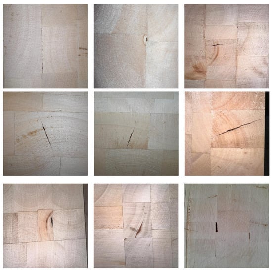
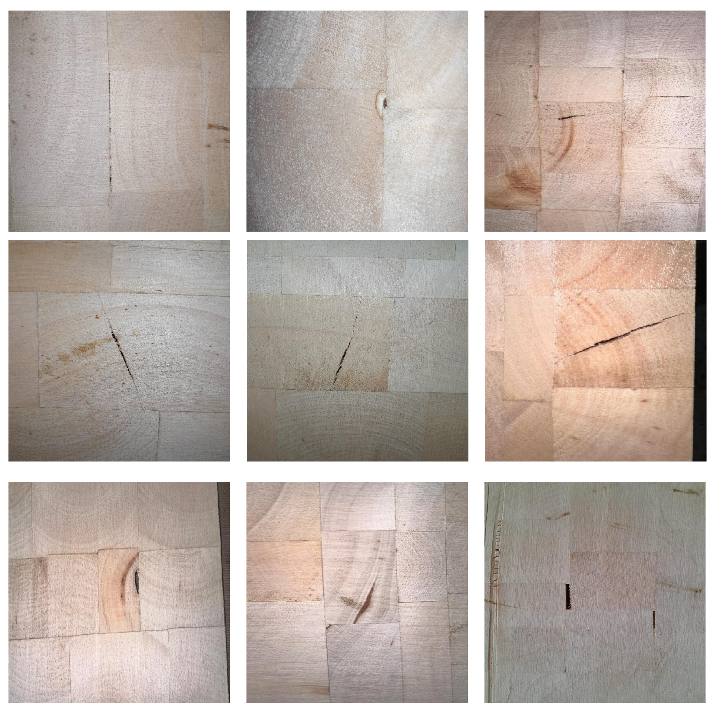
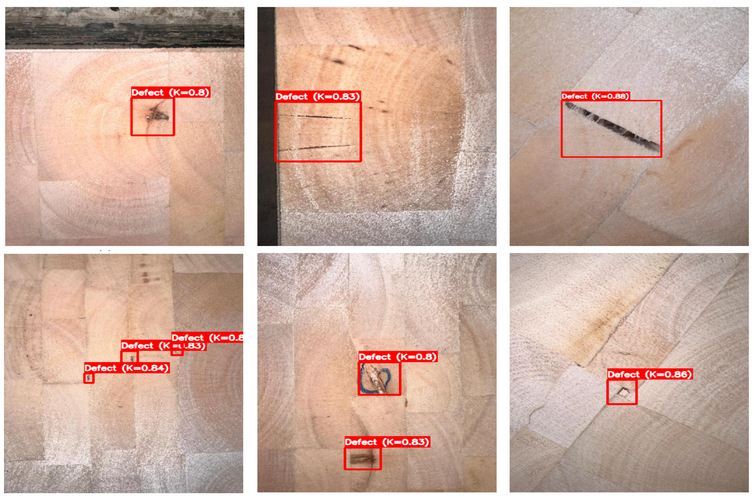
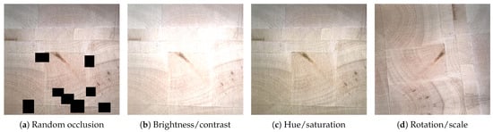
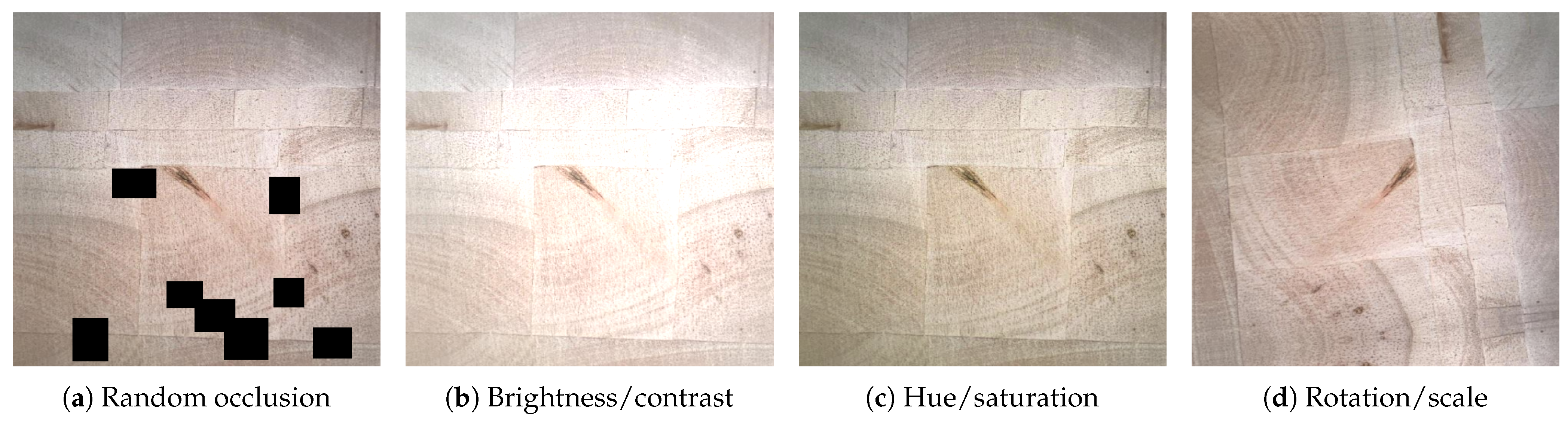
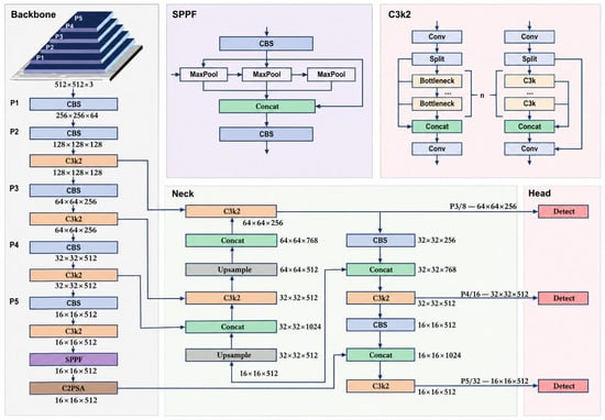
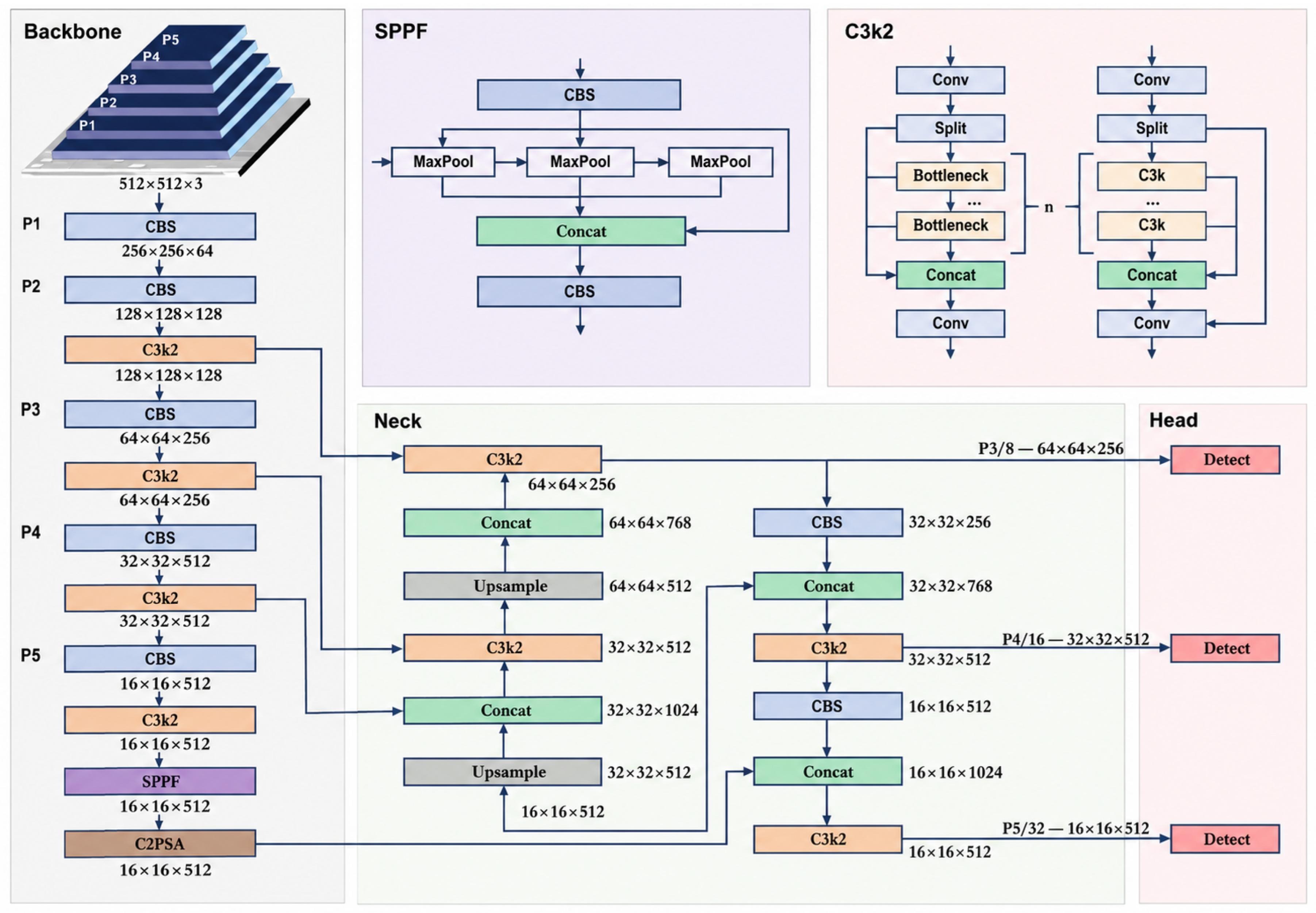
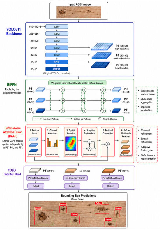
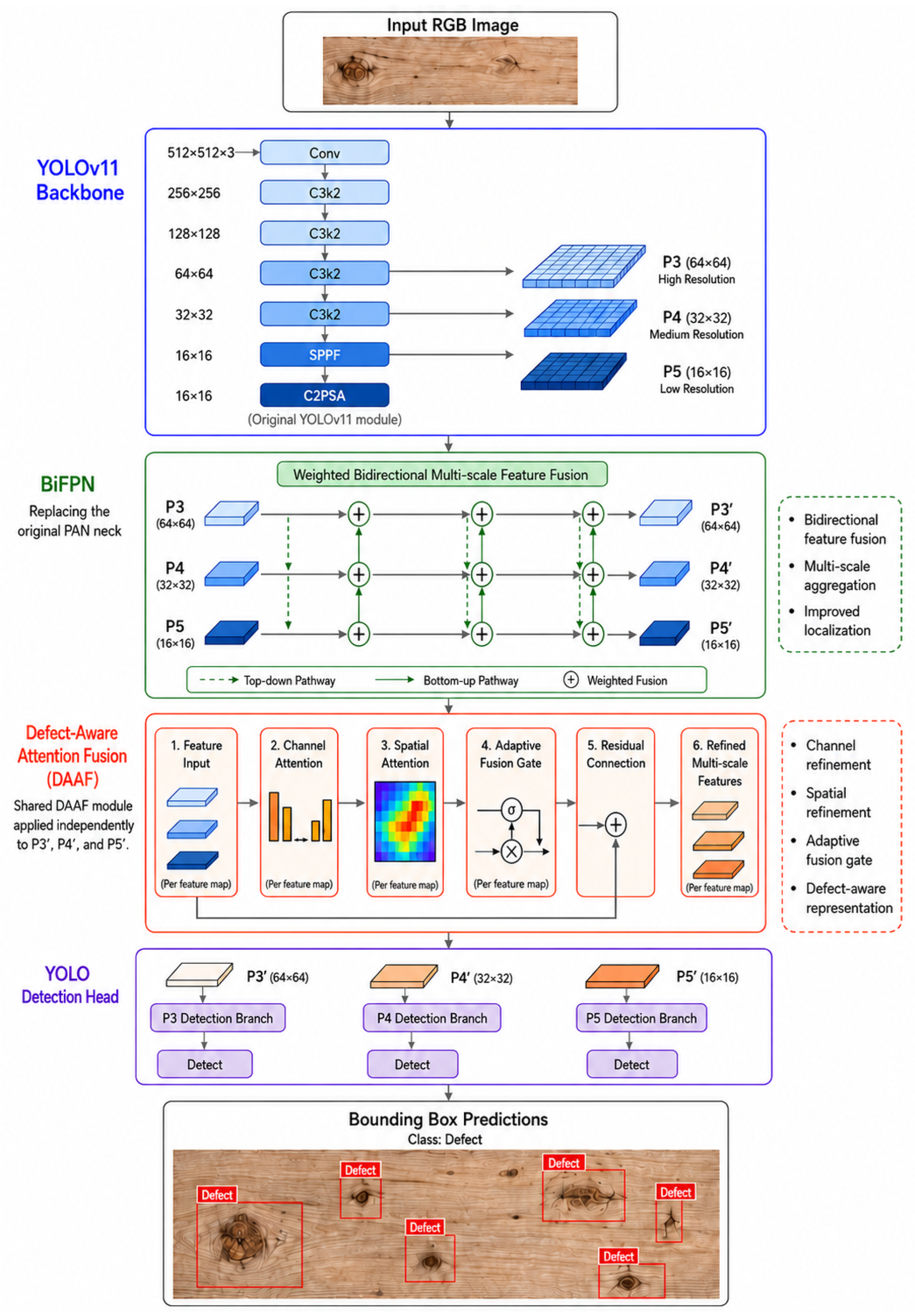
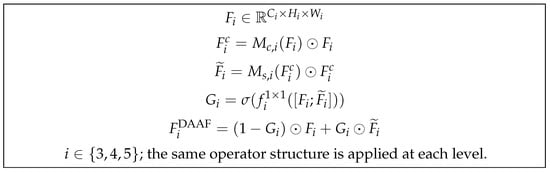
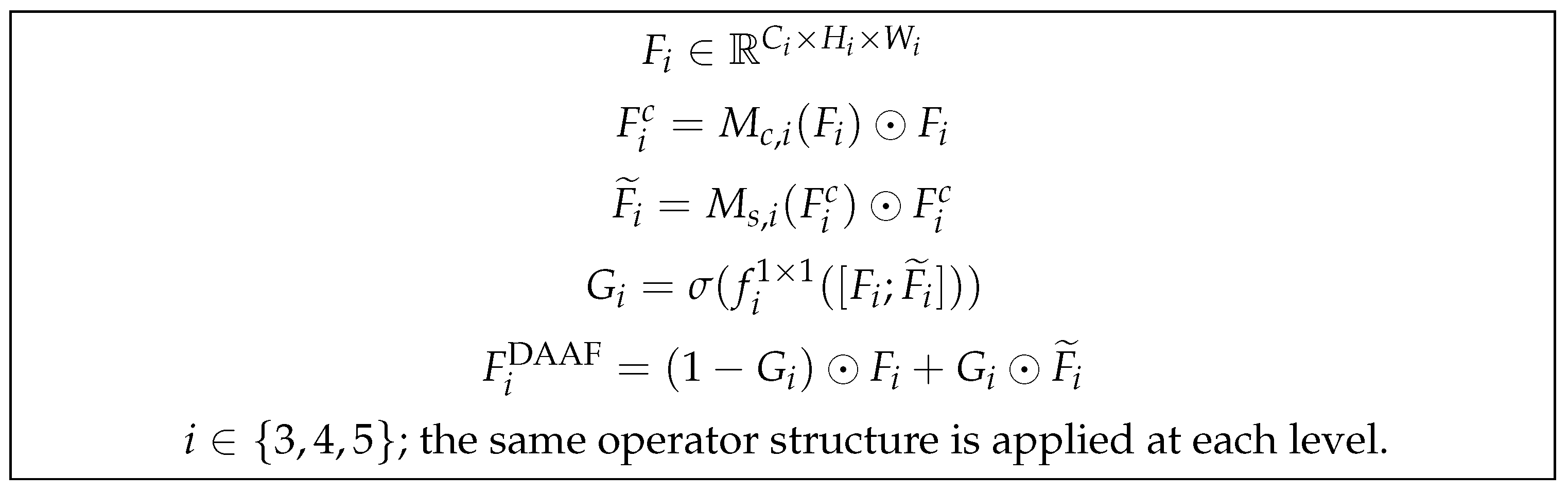
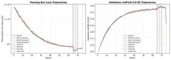
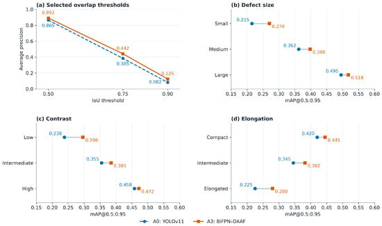
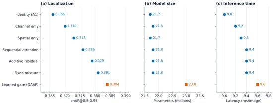
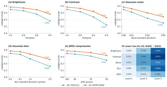
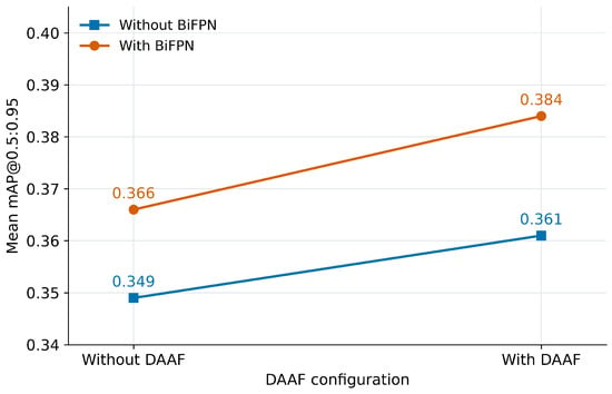
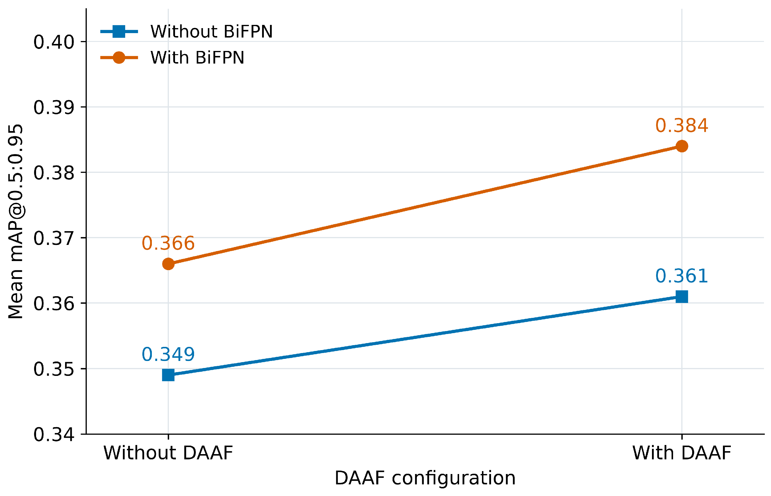
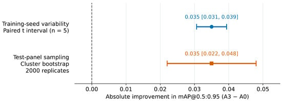
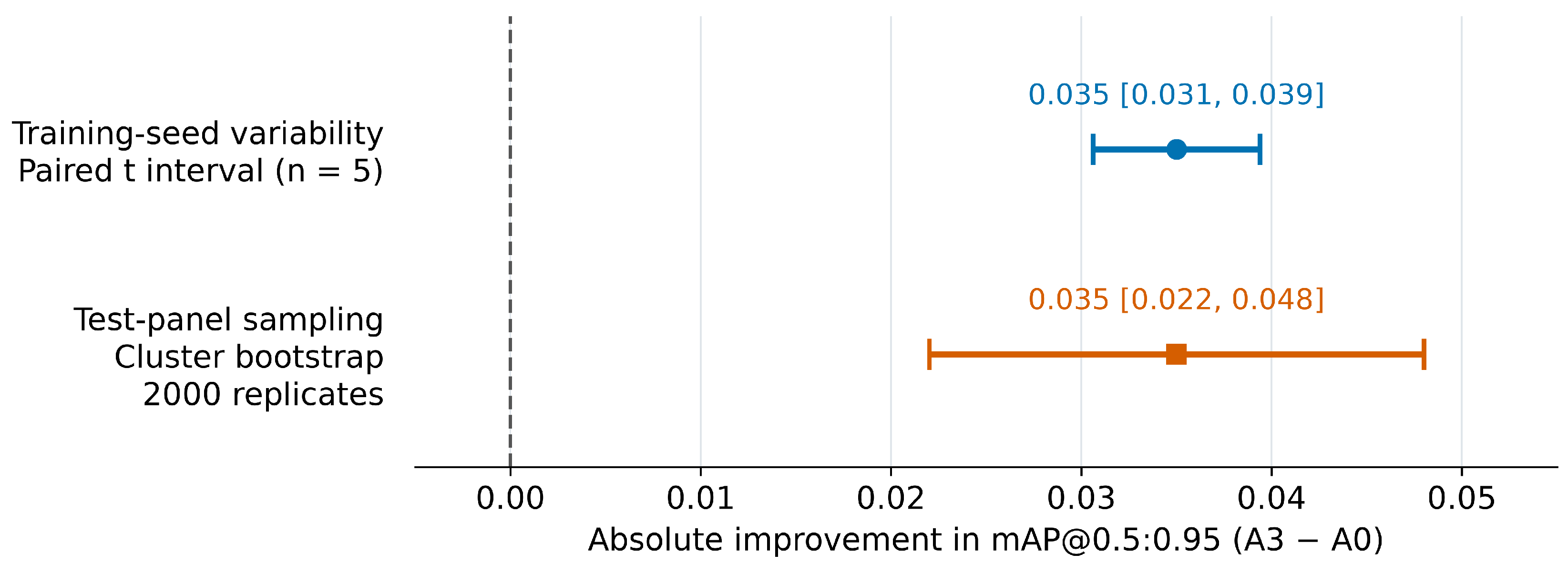
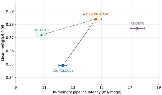
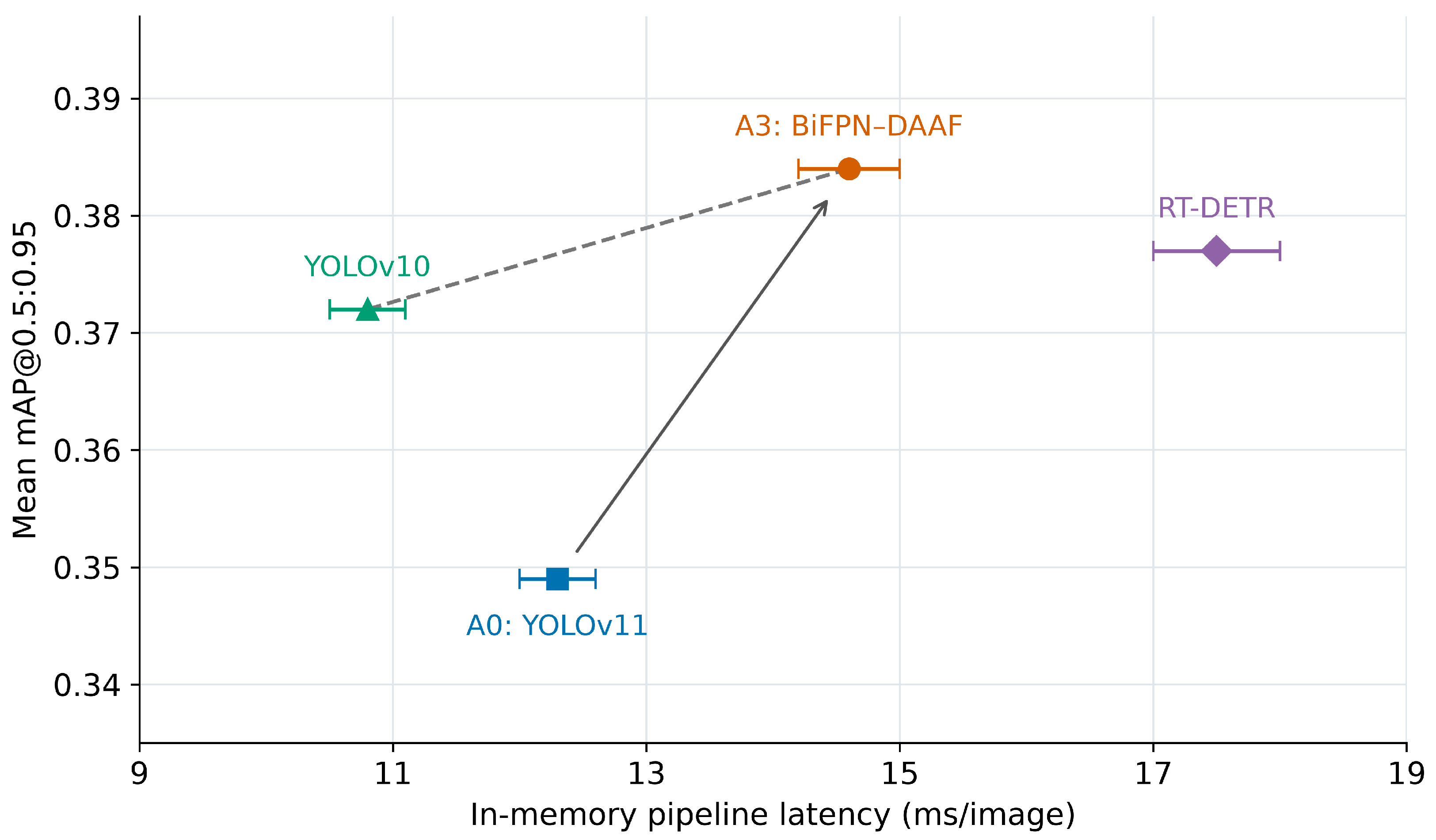
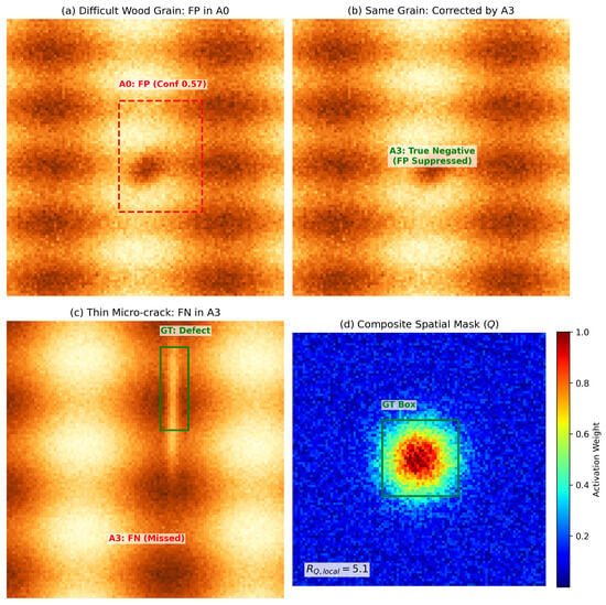
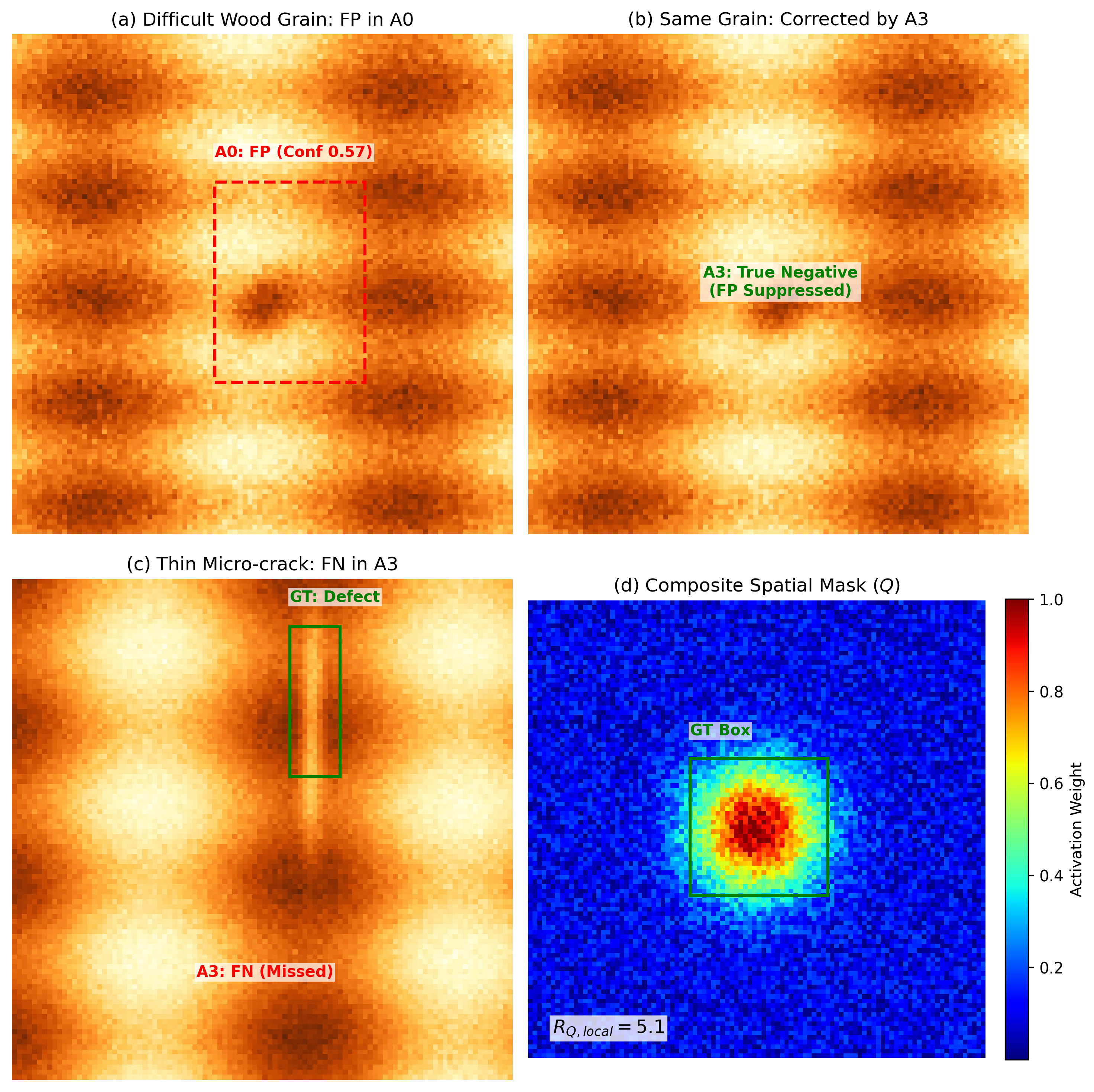

Disclaimer/Publisher’s Note: The statements, opinions and data contained in all publications are solely those of the individual author(s) and contributor(s) and not of MDPI and/or the editor(s). MDPI and/or the editor(s) disclaim responsibility for any injury to people or property resulting from any ideas, methods, instructions or products referred to in the content. |
© 2026 by the authors. Licensee MDPI, Basel, Switzerland. This article is an open access article distributed under the terms and conditions of the Creative Commons Attribution (CC BY) license.