


Abstract
Conventional acoustic level metrics quantify infrasonic magnitude but provide limited information about how low-frequency activity is organized in frequency and time. This study introduces Unit Infrasound Activity (UIA), a single-channel signal descriptor for characterizing structured activity in the 0.5–10 Hz band through three components: Strength, Regularity, and Persistence. The method was evaluated using controlled synthetic signals, a reproducible Monte Carlo dataset of 240 randomized signals, a component-ablation analysis, and recordings from contrasting real-world environments. In the Monte Carlo analysis, median UIA was monotonically associated with a predefined synthetic activity proxy (Spearman ρ = 0.855), estimated Persistence closely tracked imposed temporal presence, and dominant-frequency estimation remained accurate for stable periodic signals. Ablation analysis showed that the three components are partially dependent and that simpler combinations emphasize different signal properties, while the full formulation retains sensitivity to magnitude, temporal recurrence, and frequency stability. Application to measured recordings further showed that similar aggregate UIA values can arise from substantially different combinations of Strength, Regularity, and Persistence. UIA is therefore proposed as a complementary continuous descriptor of infrasonic signal structure rather than as a conventional sound-level measure, binary detector, source-identification method, or measure of human response.
1. Introduction
Infrasound is generally defined as acoustic energy at frequencies below 20 Hz, where human auditory sensitivity decreases substantially with decreasing frequency. Nevertheless, sufficiently high infrasonic sound pressure levels can be perceived and may produce sensations of pressure or vibration [1,2,3]. Perception thresholds vary considerably between individuals, and enhanced sensitivity to infra- and low-frequency sound has also been reported in a subgroup of individuals [1,4]. Although evidence for specific chronic health effects remains limited, reviews have reported annoyance and other self-reported responses associated with low-frequency noise and infrasound exposure [5]. These observations motivate accurate characterization of infrasonic environments but do not imply that the signal metric developed here represents human perception or health response.
Several approaches have been established for assessing low-frequency noise, but their definitions, frequency ranges, and evaluation criteria vary considerably. Common methods use equivalent sound pressure levels, frequency-weighted levels, or one-third-octave-band analysis. Occupational criteria, for example, have been proposed using one-third-octave analysis and equivalent A-weighted sound pressure levels over approximately 10–250 Hz [6]. Environmental approaches similarly differ: Danish guidelines primarily address low-frequency noise over 10–160 Hz, whereas Swedish criteria have traditionally considered one-third-octave bands between 31.5 and 200 Hz [7]. Other procedures employ C-weighted levels, differences between C- and A-weighted levels, statistical levels, or frequency-specific threshold curves [8,9]. Within the infrasonic range, ISO 7196 defines G-frequency weighting for signals containing energy between 1 and 20 Hz [10]. Thus, standardized descriptors for infrasonic sound pressure exist, including frequencies below 10 Hz. However, these measures primarily quantify signal magnitude or spectral distribution and provide limited information about temporal organization. Signals that are continuous, intermittent, irregular, or periodically recurring may therefore produce similar level-based descriptors despite substantially different temporal behavior. The methodological gap addressed here is consequently not the measurement of infrasonic amplitude itself, but the quantitative characterization of structured, regular, and persistent activity at very low frequencies.
More advanced signal-processing approaches have demonstrated that infrasonic signals contain useful temporal and spectral information beyond overall amplitude. Bishop et al. compared array-processing techniques, including frequency–wavenumber analysis, progressive multi-channel correlation, and robust regression, showing that infrasonic signals in the 0.5–3 Hz range can be characterized through spatial coherence and propagation parameters [11]. Scalar descriptors combining infrasonic amplitude and temporal occurrence have also been introduced in volcanic monitoring. Ulivieri et al. [12] introduced an Infrasonic Parameter (IP), subsequently employed by Ripepe et al. [13], defined as the product of mean infrasonic amplitude and the number of array-based detections per minute. The IP therefore combines signal magnitude with detection rate and is strongly related to the persistence of detected infrasonic activity [12,13]. More recently, Blom et al. introduced a single-channel approach based on adaptive spectrogram analysis, in which time–frequency points exceeding an estimated background level are grouped using density-based clustering to characterize infrasonic transients [14]. Other studies have combined time-, frequency-, and array-domain features with machine-learning methods for infrasonic source discrimination [15]. These approaches demonstrate that temporal and spectral information can complement conventional amplitude-based characterization. The contribution of the present work is therefore narrower: UIA is designed as a fixed-window, single-channel descriptor that combines robust signal magnitude with an explicit measure of spectral regularity and a separate measure of temporal persistence. Its intended purpose is the comparative characterization of infrasonic activity over extended measurement periods rather than event detection, source localization, classification, or source-specific warnings.
Building on this distinction, this study introduces Unit Infrasound Activity (UIA), a signal-based metric for characterizing structured infrasonic activity in the 0.5–10 Hz band. UIA combines three complementary components—Strength, Regularity, and Persistence—to distinguish signal magnitude from spectral organization and temporal recurrence.
2. Materials and Methods
2.1. Definition of Unit Infrasound Activity
The Unit Infrasound Activity (UIA) is introduced as a practical signal-based metric for characterizing and comparing persistent infrasonic activity within the 0.5–10 Hz frequency range when a common acquisition scaling is used. UIA is not a standardized sound-level metric, is not expressed in decibels, and is not intended as a measure of human perception or health effects. Regularity and Persistence are dimensionless quantities, whereas Strength retains the input waveform’s physical unit. Consequently, UIA has the same unit as Strength. For calibrated pressure recordings, S and UIA are expressed in pressure units; for uncalibrated voltage or digital-count recordings, the corresponding voltage or count units are retained. UIA values are therefore directly comparable across recordings only when the same acquisition scaling is used or when the input signals have been converted to a common physical unit.
UIA combines three signal characteristics: Strength (S), representing the typical magnitude of the infrasonic signal; Regularity (R), representing the concentration of signal energy around a dominant frequency; and Persistence (P), representing the temporal recurrence of this frequency component. For the i-th 30 s analysis window, UIA is defined as
where each 30 s window is analyzed independently. The multiplicative formulation represents joint structured activity rather than statistically independent attributes. Strength provides the magnitude term, whereas Regularity and Persistence act as dimensionless weighting factors describing spectral concentration and temporal recurrence, respectively. Because changes in temporal occupancy or frequency stability may influence more than one component, partial dependence between S, R, and P is expected. The formulation therefore does not assume statistical independence. Its behavior relative to simpler combinations of component terms is examined through an ablation analysis in Section 3.3.
UIAi = Si Ri Pi,
The zero-product property is also intentional: if no recurring dominant component is identified (P = 0), the corresponding window receives zero UIA regardless of its instantaneous magnitude. UIA should therefore be interpreted as a measure of jointly strong, regular, and persistent activity rather than total infrasonic energy.
For a measurement containing N analysis windows, the representative value for the measurement location is defined as
UIAsite = median{UIAi}, i = 1, …, N.
Thus, a longer measurement provides more observations rather than inherently producing a higher UIA. The results are reported together with the interquartile range (IQR); the individual S, R, and P components; the dominant frequency and its stability; the number of analyzed windows; and the total measurement duration.
2.2. Mathematical Definition of UIA Components
Let xi[n] denote the signal within the i-th 30 s analysis window. Before segmentation, the complete recording was centered by subtracting its median and band-pass filtered between 0.5 and 10 Hz. The filter was designed in MATLAB R2026a (The MathWorks, Inc., Natick, MA, USA) using butter(4, [0.5 10]/(Fs/2), “bandpass”), implemented in second-order-section form, and applied using forward–backward zero-phase filtering (filtfilt). To reduce the influence of short-duration high-amplitude transients, a robust center and scale were estimated independently for each 30 s window. The window median mi and median absolute deviation (MAD) [16] were calculated as
and the robust scale was defined as σr,i = 1.4826 MADi. Samples outside mi ± 8σr,i were clipped to the corresponding lower or upper limit rather than removed. This procedure preserves the duration and temporal alignment of each analysis window while limiting the influence of isolated extreme amplitudes.
mi = median{xi[n]},
MADi = median{|xi[n] − mi|},
2.2.1. Strength
Strength represents the typical magnitude of the filtered infrasonic fluctuations after transient limitation. For the resulting robust signal i[n], Strength is defined as
The median absolute amplitude is used instead of peak or root-mean-square amplitude to reduce the influence of residual high-amplitude events. Because no normalization is applied to S, its numerical magnitude depends on the input waveform scaling. R and P modulate this magnitude according to spectral regularity and temporal persistence but do not alter its physical units.
2.2.2. Regularity
The power spectral density (PSD) of each 30 s window is estimated using Welch’s averaged periodogram method [17]. For the 30 s analysis windows, Welch PSD estimates were calculated using a 10 s Hann window with 50% overlap and an NFFT corresponding to 20 s of data. At Fs = 1060 samples/s, these settings correspond to 10,600 samples per Welch segment, 5300 samples of overlap, and NFFT = 21,200, yielding a frequency spacing of 0.05 Hz. MATLAB’s pwelch function was used with PSD scaling. No additional explicit detrending was applied prior to pwelch beyond the median centering performed before band-pass filtering:
The dominant infrasonic frequency is defined as the frequency corresponding to the maximum PSD within the analysis band:
Regularity is defined as the fraction of the total spectral energy concentrated within ±0.15 Hz of the dominant frequency:
When the ±0.15 Hz interval extends beyond the 0.5–10 Hz analysis band, the integration limits are truncated at the corresponding band boundary. Thus, the numerator is evaluated only over the portion of the interval contained within 0.5–10 Hz. Accordingly, 0 ≤ Ri ≤ 1. Broadband or irregular activity produces a low Ri, whereas a signal dominated by a stable narrowband component approaches unity.
2.2.3. Persistence
Persistence determines whether the dominant spectral component observed in the 30 s window is repeatedly present over time. Each window is divided into six non-overlapping 5 s segments. For segment j, the dominant frequency fi,j* and its corresponding spectral peak are determined. A segment is considered active when
and
|fi,j* − fi*| ≤ 0.20 Hz,
For each 5 s sub-window, the PSD was estimated using a Hann window spanning the complete sub-window, with zero overlap, and the same 20 s NFFT used in the 30 s spectral analysis. The spectral background Bi,j was defined as the median PSD over the 0.5–10 Hz analysis band after excluding frequencies within ±0.40 Hz of the 30 s dominant frequency fi. A candidate peak had to lie within ±0.20 Hz of fi and exceed this spectral background by a factor of at least 2.5. With Ii,j defined as 1 when both conditions are satisfied and 0 otherwise, Persistence is
Pi = (1/6) Σj=16 Ii,j.
Consequently, Pi ranges from 0 to 1 and directly represents the fraction of subsegments in which the dominant infrasonic component persists.
The selected window durations, frequency tolerances, and peak-to-background criterion are operational parameters of the present UIA implementation rather than theoretically unique or universally optimized constants. The 30 s analysis window defines the interval over which spectral concentration is characterized, while its division into six 5 s segments provides a measure of within-window recurrence. The ±0.15 Hz bandwidth defines spectral concentration around the dominant frequency for Regularity, whereas the slightly broader ±0.20 Hz tolerance permits limited variation in the dominant component between persistence segments. The peak-to-background ratio of 2.5 prevents weak local spectral maxima from being counted as persistent activity. These baseline parameters were held fixed throughout the primary synthetic and measured data analyses. A limited one-at-a-time robustness analysis was additionally performed to examine whether the principal synthetic-evaluation results depended strongly on moderate variation in the operational settings; this analysis was not used to optimize the baseline configuration. Systematic optimization and evaluation of transferability across different signal environments and acquisition systems remain subjects for future work.
For reproducibility, the fixed signal-processing parameters used in the present implementation are summarized in Table 1. These settings were applied consistently throughout the UIA calculations unless otherwise stated. The sampling frequency used for the measurements and synthetic signals was 1060 samples/s.
Table 1.
Fixed signal-processing parameters used for UIA calculation.
2.3. UIA Algorithm
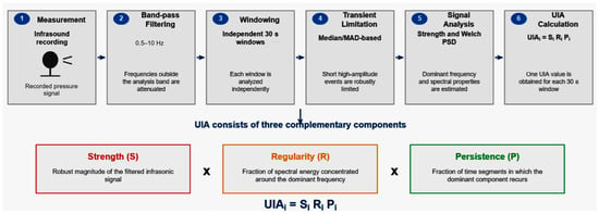
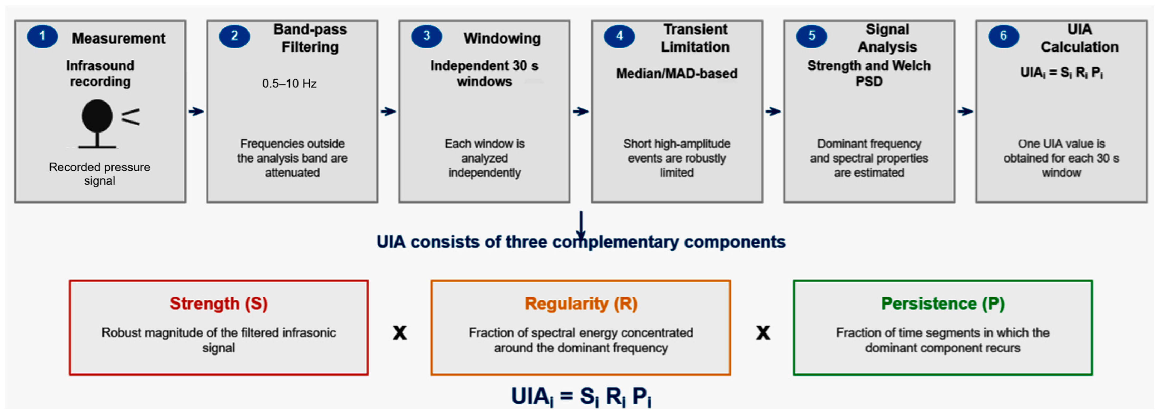
The complete UIA procedure is summarized in Algorithm 1, while Figure 1 provides an overview of the processing workflow. Each 30 s interval is treated as an independent observation, and the final value for a measurement location is obtained from the distribution of the individual UIA values.
Figure 1.
Calculation of Unit Infrasound Activity (UIA): Processing workflow from recorded infrasonic signal to the final UIA descriptor.
The operations in Algorithm 1 correspond directly to the signal-processing definitions in Section 2.2. Specifically, BANDPASS applies the filtering procedure described in Section 2.2, LIMIT_TRANSIENTS applies the MAD-based transient-limitation procedure defined by Equations (3) and (4) and the subsequent clipping rule, and LOCAL_SPECTRAL_BACKGROUND uses the background calculation defined in Section 2.2.3. The calculations of Strength, Regularity, and Persistence otherwise follow their respective definitions in Section 2.2.1, Section 2.2.2 and Section 2.2.3.
| Algorithm 1. Unit Infrasound Activity (UIA) | |
| Input: Recorded signal x[n], sampling frequency Fs | |
| Output: UIA values and summary statistics | |
| 01 | procedure UIA(x[n], Fs) |
| 02 | x ← BANDPASS(x, 0.5, 10, Fs) |
| 03 | W ← DIVIDE_INTO_WINDOWS(x, 30 s) |
| 04 | for each window Wi in W do |
| 05 | mi ← MEDIAN(Wi) |
| 06 | MADi ← MEDIAN(|Wi − mi|) |
| 07 | i ← LIMIT_TRANSIENTS(Wi, mi, MADi) |
| 08 | Si ← MEDIAN(|i|) |
| 09 | PSDi ← WELCH(i) |
| 10 | fi* ← DOMINANT_FREQUENCY(PSDi, 0.5–10 Hz) |
| 11 | Ri ← SPECTRAL_ENERGY(PSDi, fi* ± 0.15 Hz)/SPECTRAL_ENERGY(PSDi, 0.5–10 Hz) |
| 12 | segments ← DIVIDE_INTO_SEGMENTS(i, 5 s) |
| 13 | count ← 0 |
| 14 | for each segment j do |
| 15 | fj* ← DOMINANT_FREQUENCY(segment j) |
| 16 | Bj ← LOCAL_SPECTRAL_BACKGROUND(segment j) |
| 17 | if |fj* − fi*| ≤ 0.20 Hz and PEAK(fj*)/Bj ≥ 2.5 then |
| 18 | count ← count + 1 |
| 19 | end if |
| 20 | end for |
| 21 | Pi ← count/6 |
| 22 | UIAi ← Si Ri Pi |
| 23 | end for |
| 24 | UIAsite ← MEDIAN({UIAi}) |
| 25 | IQRsite ← IQR({UIAi}) |
| 26 | return UIAsite, IQRsite, {Si, Ri, Pi, fi*} |
| 27 | end procedure |
2.4. Reproducible Monte Carlo Simulation Protocol
A reproducible Monte Carlo simulation was used to evaluate the behavior of UIA across a broad range of controlled signal conditions. A total of 240 independent synthetic recordings were generated, each 6 min long and sampled at 1060 samples/s. Of these, 180 contained a periodic infrasonic component, and 60 served as null signals containing background noise and transient contamination but no periodic component. Random-number generation used the MATLAB Mersenne Twister generator with a fixed seed of 20260928.
The 240 Monte Carlo recordings were generated independently of the 12 controlled synthetic signals examined in Section 3.1, with no shared signal realizations; both datasets were analyzed using the same fixed UIA processing parameters.
For signal-containing realizations, amplitude was sampled from a log-uniform distribution between 0.008 and 0.14, temporal presence from a uniform distribution between 0.10 and 1.00, dominant frequency from a uniform distribution between 0.5 and 8.5 Hz, and frequency-jitter standard deviation from a uniform distribution between 0 and 0.35 Hz. Background Gaussian-noise standard deviation was sampled uniformly between 0.015 and 0.060. Transient contamination was generated at rates uniformly distributed between 0 and 6 events/min, with event durations between 0.02 and 0.20 s and amplitudes between 6 and 20 times the larger of the periodic-signal amplitude and background-noise standard deviation.
Temporal presence was implemented using randomly selected 5 s blocks. For each active block, an independent Gaussian frequency offset with the prescribed jitter standard deviation was applied to the nominal dominant frequency. Null realizations were generated using the same noise and transient procedures but without a periodic component. All synthetic recordings were analyzed using the fixed UIA implementation and parameters summarized in Table 1, without adjustment based on the simulation outcomes.
2.5. Field Measurements and Instrumentation
Field recordings were acquired using the same 65 mm Lidström infrasound microphone (Gargnäs Electronics, Skellefteå, Sweden), the same sampling frequency of 1060 samples/s, and the same acquisition configuration at all measurement locations. The sensor provides a measurable response within the frequency range considered in the present analysis, including frequencies down to approximately 0.5 Hz. Before each measurement, the instrumentation was allowed to stabilize for approximately 20 min. For outdoor measurements, the microphone was positioned at ground level and protected by a metal windscreen, whereas for indoor residential measurements it was positioned on the floor.
The field recordings were selected to represent contrasting infrasonic signal environments rather than to determine absolute sound-pressure exposure or source-emission levels. Fiby represented an outdoor reference environment without a known local infrasound source; the turbine recordings represented an outdoor known-source condition and were obtained at a standardized measurement distance while the respective wind turbines were operating; Villa represented an indoor residential environment containing persistent infrasonic activity of unidentified origin; and the apartment recording provided a separate indoor residential comparison. The same instrumentation and UIA-processing procedure were applied throughout. Meteorological conditions were not systematically included as experimental variables. Consequently, wind-induced pressure fluctuations and atmospheric variability cannot be separated from other signal components in the outdoor recordings, and these measurements are interpreted as characterizations of the measured infrasonic signal environment rather than as source-specific emission measurements.
The field measurements in both experiments were obtained using the Lidström infrasound microphone and analyzed in the original voltage domain (V), without conversion to acoustic pressure. Accordingly, Strength and UIA are expressed in volts for the reported field results, whereas Regularity and Persistence are dimensionless. For graphical comparison of the three components, Strength was normalized relative to the maximum median Strength across the recordings included in each figure. This normalization was applied only for visualization and did not affect the calculated UIA values.
3. Results and Discussion
3.1. Controlled Synthetic-Signal Evaluation
The UIA method was initially evaluated using a controlled set of 12 synthetic signals for which the underlying signal characteristics were known a priori. Each signal had a duration of 12 min and was generated at a sampling frequency of 1060 samples/s. The test set was designed to challenge the main properties represented by UIA, including signal magnitude, temporal persistence, frequency stability, frequency location within the 0.5–10 Hz analysis band, and robustness to transient disturbances.
The synthetic dataset included a noise-only negative control, noise containing isolated high-amplitude transients, weak and moderate 1 Hz signals with different temporal occupancies (25%, 50%, and 100%), and a strong persistent 1 Hz signal. Additional signals were generated to test frequency instability, persistent activity at 0.65 and 6.2 Hz, and recovery of a persistent 1 Hz component in the presence of strong transient disturbances. Background noise was included in all relevant test cases.
All signals were processed using the predefined UIA algorithm without parameter adjustment based on the validation results. Performance was evaluated using three complementary criteria: (1) agreement between known and estimated Persistence, (2) absolute error between the imposed and recovered dominant frequency for periodic test signals, and (3) monotonic agreement between UIA and a known activity proxy defined from the imposed signal amplitude and temporal presence. The validation was therefore designed to determine whether UIA responds predictably to controlled changes in signal strength, persistence, and regularity while remaining robust to broadband noise and isolated transient events.
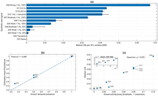
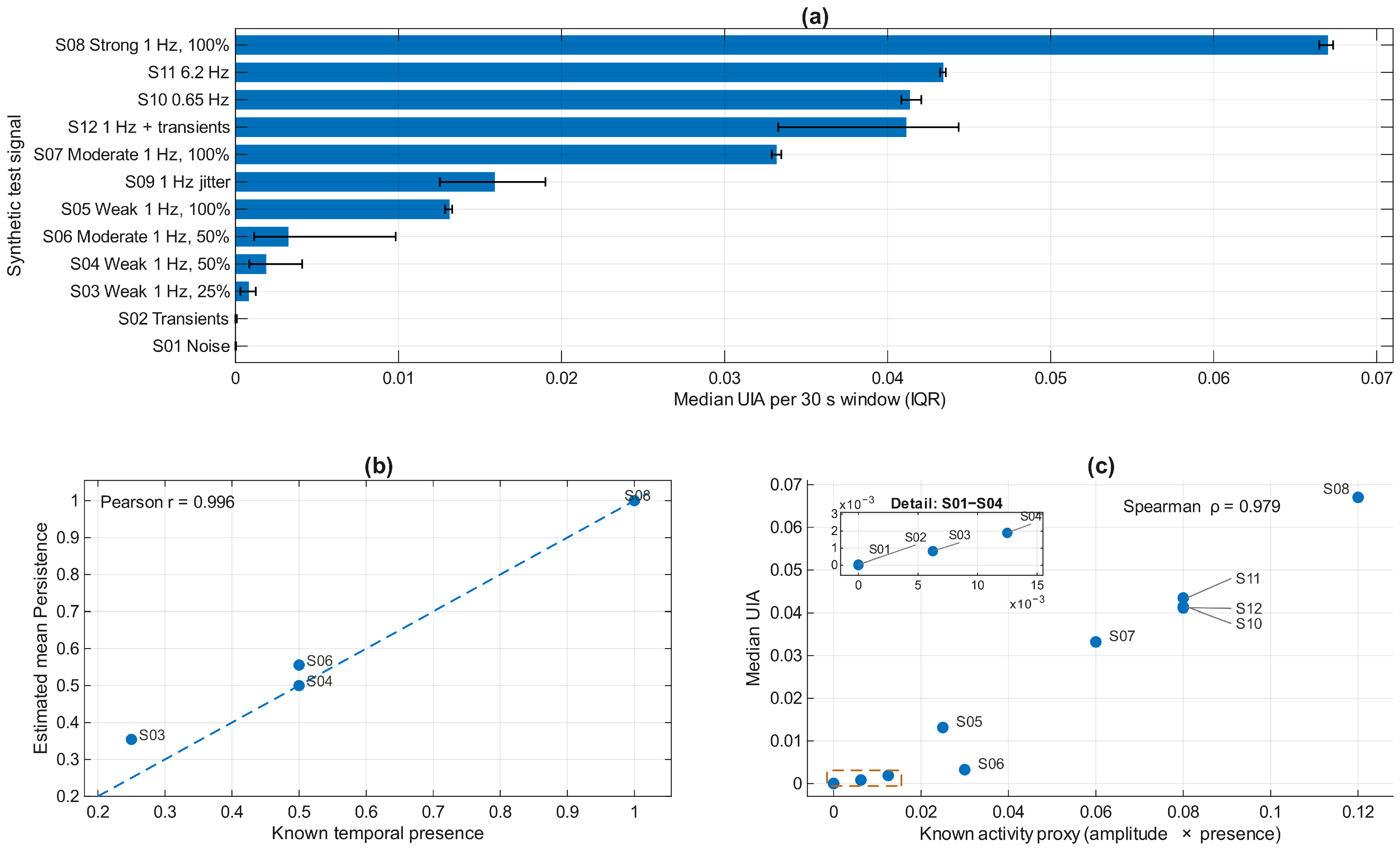
Table 2 demonstrates that the proposed UIA method responds systematically to controlled variations in infrasonic activity. The noise-only signal produced a median UIA of zero, while adding isolated high-amplitude transients resulted in only a negligible increase (0.00003), indicating that transient events alone were not interpreted as persistent infrasonic activity. For weak 1 Hz signals, increasing the known temporal presence from 25% to 50% and 100% increased both Persistence and median UIA. A corresponding amplitude-dependent response was observed for fully persistent 1 Hz signals, for which the median UIA increased from 0.01313 for the weak signal to 0.03320 and 0.06702 for the moderate and strong signals, respectively.
Table 2.
Controlled synthetic-signal evaluation of the UIA method.
The controlled synthetic-signal experiments demonstrate that UIA responds systematically to the signal characteristics it was designed to quantify. As shown in Figure 2a, the noise-only condition produced essentially zero UIA, while isolated high-amplitude transients resulted in only a negligible response. In contrast, the introduction of persistent periodic components produced progressively larger UIA values as temporal presence and signal magnitude increased. Fully persistent signals at 0.65, 1.0, and 6.2 Hz all produced substantial UIA values, showing that such values were obtained for stable persistent signals at different frequencies within the defined 0.5–10 Hz analysis range.
Figure 2.
Controlled synthetic-signal evaluation of the proposed UIA method. (a) Median UIA across independent 30 s analysis windows for the 12 synthetic test signals; error bars indicate the interquartile range. (b) Agreement between known temporal presence and estimated mean Persistence for signals specifically generated with controlled temporal occupancy. The dashed line indicates identity. (c) Relationship between the predefined activity proxy, calculated as imposed signal amplitude multiplied by temporal presence, and median UIA for the standard activity test cases. Special robustness cases involving isolated transients, strong frequency jitter, or transient contamination of a persistent signal were evaluated separately and were not included in the monotonicity correlation.
The Persistence component closely followed the imposed temporal occupancy of the controlled 1 Hz signals (Figure 2b). Across the signals specifically designed for this test, known temporal presence and estimated mean Persistence showed a strong linear association (Pearson r = 0.996). Signals present throughout the complete recording approached a Persistence value of 1, whereas partially present signals produced correspondingly lower estimates. This result supports the ability of the subwindow-based procedure to quantify the temporal recurrence of a stable infrasonic component.
Median UIA also exhibited a strong monotonic relationship with the predefined activity proxy (Figure 2c), with Spearman ρ = 0.979. The result indicates that increasing the combination of signal magnitude and temporal presence generally produces increasing UIA without requiring a linear relationship between the variables. The dedicated robustness cases further showed that isolated transients alone did not generate substantial UIA, whereas the underlying persistent 1 Hz component continued to produce a substantial UIA response in the presence of strong transient contamination. Conversely, deliberate frequency jitter reduced both Persistence and the resulting UIA, consistent with the intended sensitivity of the metric to regular, recurring infrasonic activity.
3.2. Monte Carlo Evaluation
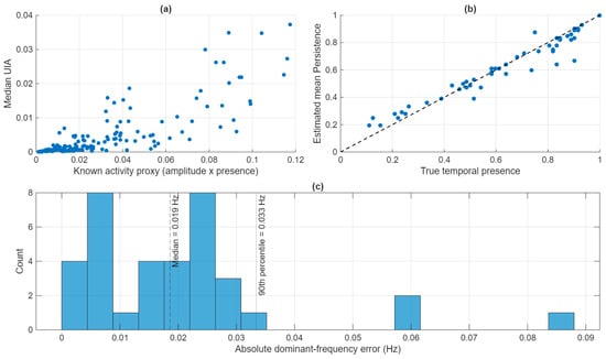
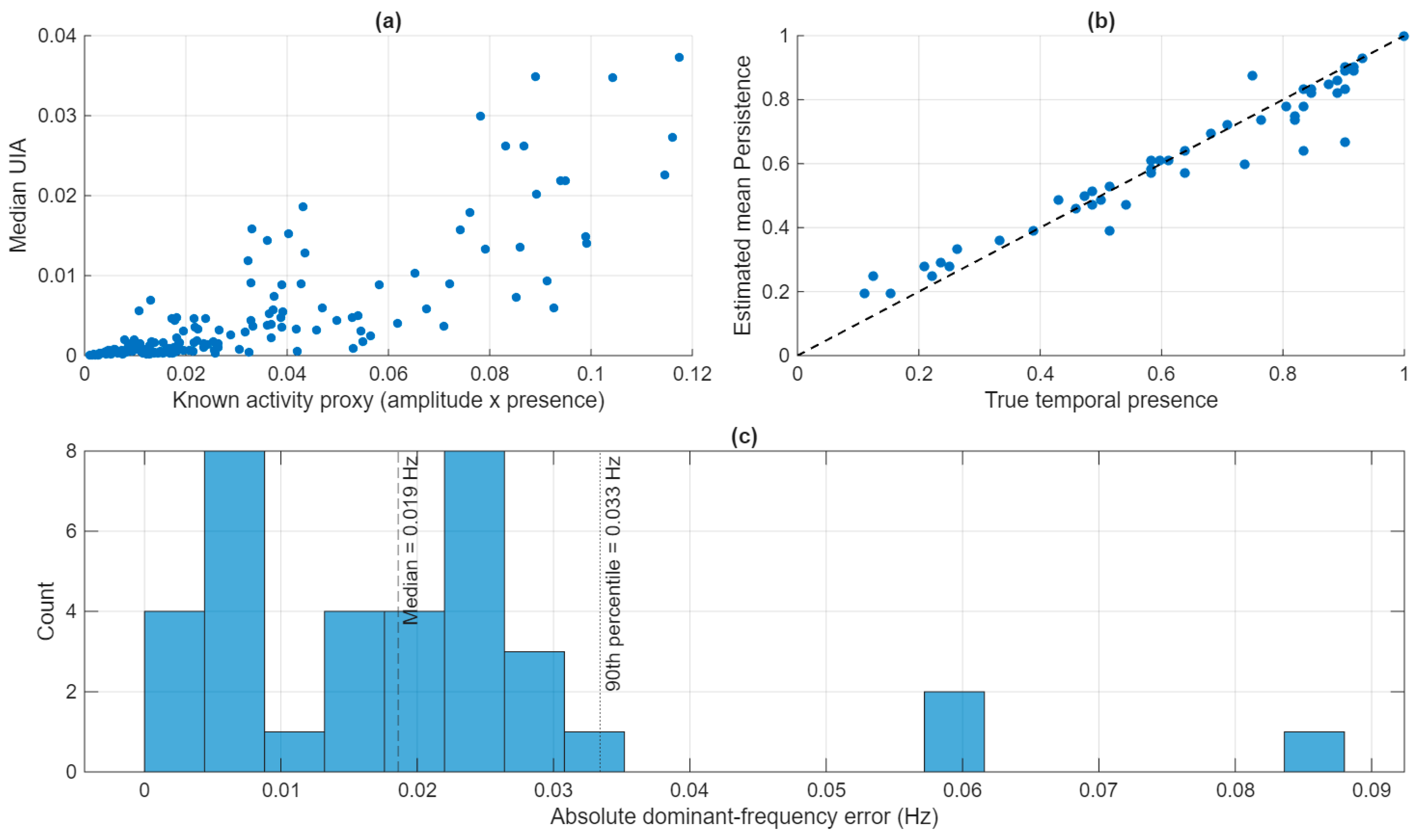
To evaluate the robustness of UIA across a broader range of signal conditions than those represented by the controlled test cases, the reproducible Monte Carlo dataset described in Section 2.4 was analyzed using the fixed UIA implementation. The validation assessed four aspects of performance: the monotonic response of UIA to increasing signal activity, recovery of temporal presence through the Persistence component, estimation of dominant frequency, and behavior under null and structured-signal conditions. The principal validation results are summarized in Table 3 and Figure 3.
Table 3.
Monte Carlo evaluation of the UIA Method.
Figure 3.
Reproducible Monte Carlo evaluation of the proposed UIA method using 240 synthetic signals. (a) Relationship between the predefined activity proxy (signal amplitude × realized temporal presence) and median UIA for the signal-containing simulations (Spearman ρ = 0.855). (b) Agreement between true temporal presence and estimated mean Persistence for the predefined persistence-validation subset (Pearson r = 0.968); the dashed line indicates identity. (c) Distribution of the absolute dominant-frequency estimation error for the predefined stable structured-signal subset. The median absolute error was 0.0186 Hz, and the 90th-percentile error was 0.0334 Hz. The complete MATLAB code for reproducible generation and analysis of the 240 synthetic recordings is provided as Supplementary Code S1.
Across the 180 signal-containing realizations, median UIA showed a strong monotonic association with the known activity proxy, defined as signal amplitude multiplied by realized temporal presence (Spearman ρ = 0.855; Figure 3a). The association was observed despite simultaneous variation in dominant frequency, frequency jitter, background noise, and transient contamination. The dispersion visible at comparable activity-proxy values is expected because UIA additionally incorporates spectral Regularity and Persistence rather than depending solely on signal amplitude and temporal presence.
The Persistence component closely tracked the imposed temporal presence for the predefined persistence-validation subset (Pearson r = 0.968; Figure 3b). Dominant-frequency estimation was also accurate for the predefined stable structured-signal subset, with a median absolute error of 0.0186 Hz and a 90th-percentile error of 0.0334 Hz (Figure 3c). These results indicate that the temporal and spectral components of UIA recover their corresponding simulated signal characteristics accurately under the evaluated conditions.
The null-signal analysis provided an additional assessment of robustness to background noise and transient contamination. None of the 60 null simulations produced a median UIA ≥ 0.002. This result characterizes the behavior of the metric under the specific null conditions used in the simulation and should not be interpreted as establishing a universal detection threshold. Taken together, the Monte Carlo results demonstrate the expected response of the UIA formulation under controlled synthetic conditions with known signal properties. They do not constitute an estimate of real-world detection performance.
3.3. Component Dependence and Ablation Analysis
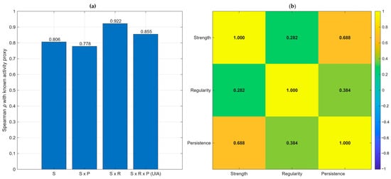
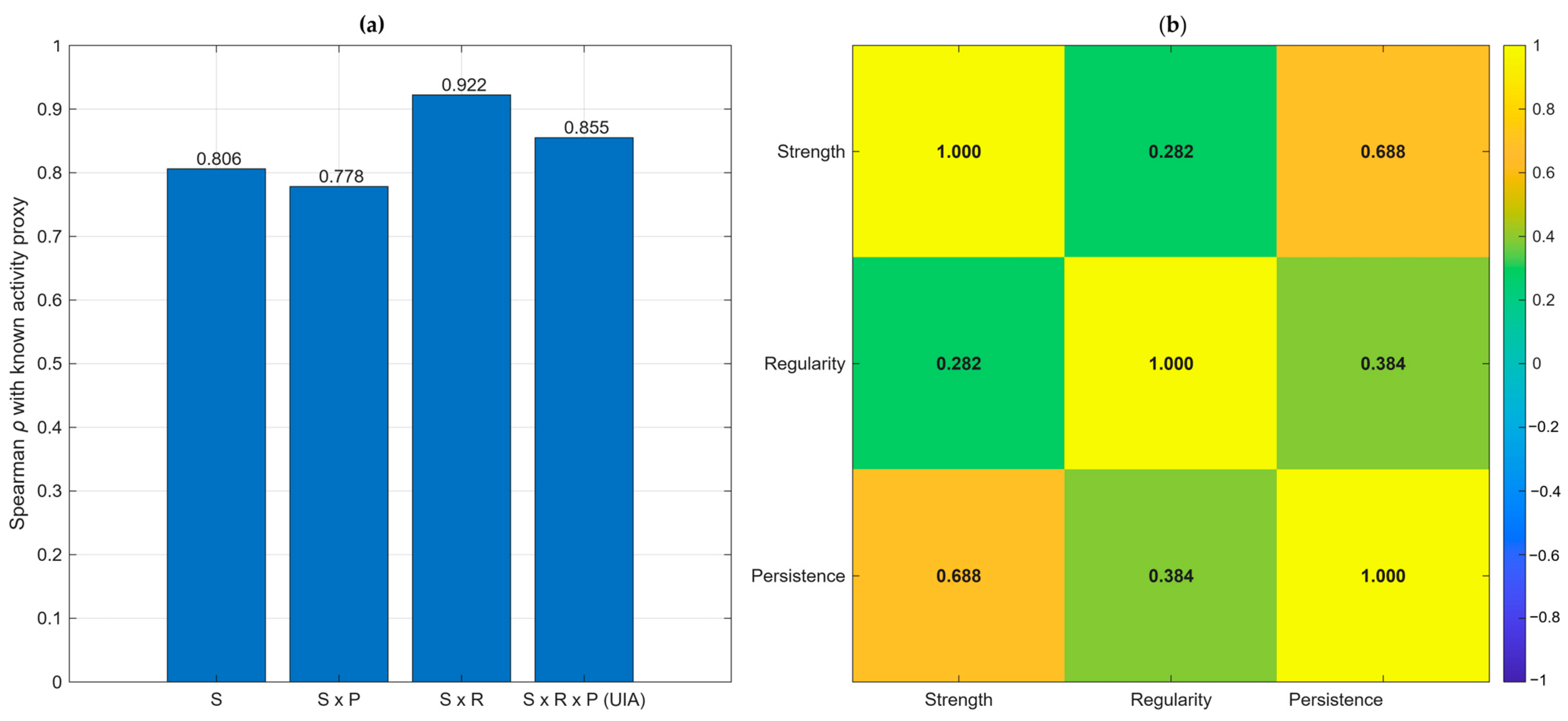
To examine whether the three UIA components provide distinct information and to assess the effect of the multiplicative formulation, an ablation analysis was performed using the reproducible Monte Carlo dataset. Four descriptors were compared: Strength alone (S), S × P, S × R, and the full UIA formulation S × R × P. Each descriptor was first calculated at the 30 s window level and subsequently summarized by the median across each simulated recording, consistent with the definition of UIA. The ablation results showed that all four descriptors retained a strong monotonic association with the predefined activity proxy (Table 4, Figure 4a). Strength alone yielded Spearman ρ = 0.806. Adding Persistence produced ρ = 0.778, whereas adding Regularity produced the strongest association with the activity proxy (ρ = 0.922). The full UIA formulation yielded ρ = 0.855. The higher correlation obtained for S × R should be interpreted in relation to the definition of the activity proxy, which contains amplitude and temporal presence but does not explicitly represent frequency instability.
Table 4.
Ablation analysis of UIA component combinations.
Figure 4.
Component-dependence and ablation analysis of UIA using the reproducible Monte Carlo dataset. (a) Spearman correlation between the predefined activity proxy and four alternative descriptors: S, S × P, S × R, and the complete S × R × P formulation. (b) Signal-level Spearman correlation matrix for Strength, Regularity, and Persistence. The results indicate partial dependence between the components, particularly between Strength and Persistence, while Regularity and Persistence remain only moderately correlated.
The secondary parameter analysis revealed complementary behavior among the descriptors. S × P showed the strongest association with imposed temporal presence (ρ = 0.860), whereas S × R showed the strongest association with imposed amplitude (ρ = 0.713). The complete UIA showed a strong association with temporal presence (ρ = 0.792) while exhibiting the strongest negative association with imposed frequency jitter (ρ = −0.226). Thus, the different component combinations emphasize different signal properties: S × P was most strongly associated with temporal presence, S × R with amplitude, and the full UIA showed the largest negative association with imposed frequency jitter among the tested combinations.
The UIA components were partially correlated but not redundant (Figure 4b). At the signal level, the Spearman correlations were ρ = 0.282 between Strength and Regularity, ρ = 0.688 between Strength and Persistence, and ρ = 0.384 between Regularity and Persistence. The comparatively stronger S–P relationship is consistent with the expectation that reduced temporal occupancy can influence both typical signal magnitude and estimated Persistence. However, the substantially lower R–P correlation indicates that spectral concentration and temporal recurrence retain distinct information.
These results support interpreting UIA as a deliberately composite descriptor rather than as a statistically independent factor model. The multiplicative construction imposes the requirement that appreciable magnitude, spectral organization, and temporal recurrence occur jointly. The ablation analysis also shows that simpler combinations may be preferable when only a specific signal property is of interest; the full UIA is retained because its intended purpose is to summarize all three properties simultaneously.
3.4. Parameter Robustness Analysis
A limited one-at-a-time robustness analysis was performed to examine whether the principal synthetic-evaluation results depended critically on the selected operational parameters. The Regularity bandwidth, Persistence frequency tolerance, peak-to-background criterion, analysis-window duration, and Persistence-segment duration were varied individually around the baseline configuration while the same 240 synthetic recordings were analyzed in every case.
Across the tested configurations (Table 5), the Spearman association between the predefined activity proxy and median UIA varied from 0.842 to 0.873, compared with 0.855 for the baseline configuration. Persistence recovery remained high, with Pearson r ranging from 0.938 to 0.976 relative to the baseline value of 0.968. Variations in the Regularity bandwidth and peak-to-background ratio produced only minor changes in these metrics. Changing the Persistence frequency tolerance produced somewhat larger but still moderate effects, consistent with its direct role in defining temporal recurrence.
Table 5.
One-at-a-Time Robustness Analysis of UIA Operational Parameters.
Analysis-window duration affected dominant-frequency estimation more noticeably. The 20 s configuration reduced the median absolute frequency error from 0.0186 to 0.0117 Hz and the 90th-percentile error from 0.0334 to 0.0264 Hz, whereas the 60 s configuration yielded the same median error of 0.0117 Hz but a slightly larger 90th-percentile error of 0.0352 Hz. Increasing the Persistence-segment duration from 5 to 10 s increased the activity-proxy association to 0.873 but reduced Persistence recovery to r = 0.938.
These results indicate that the principal behavior of UIA is preserved under moderate one-at-a-time variation in the selected operational parameters, although temporal segmentation and frequency-tolerance settings influence specific aspects of the metric. The analysis is intended as a robustness assessment rather than parameter optimization; the baseline settings were retained throughout the main analysis.
3.5. Experimental Evaluation Using Real Infrasound Recordings
3.5.1. Comparative Analysis of Three Measurement Environments
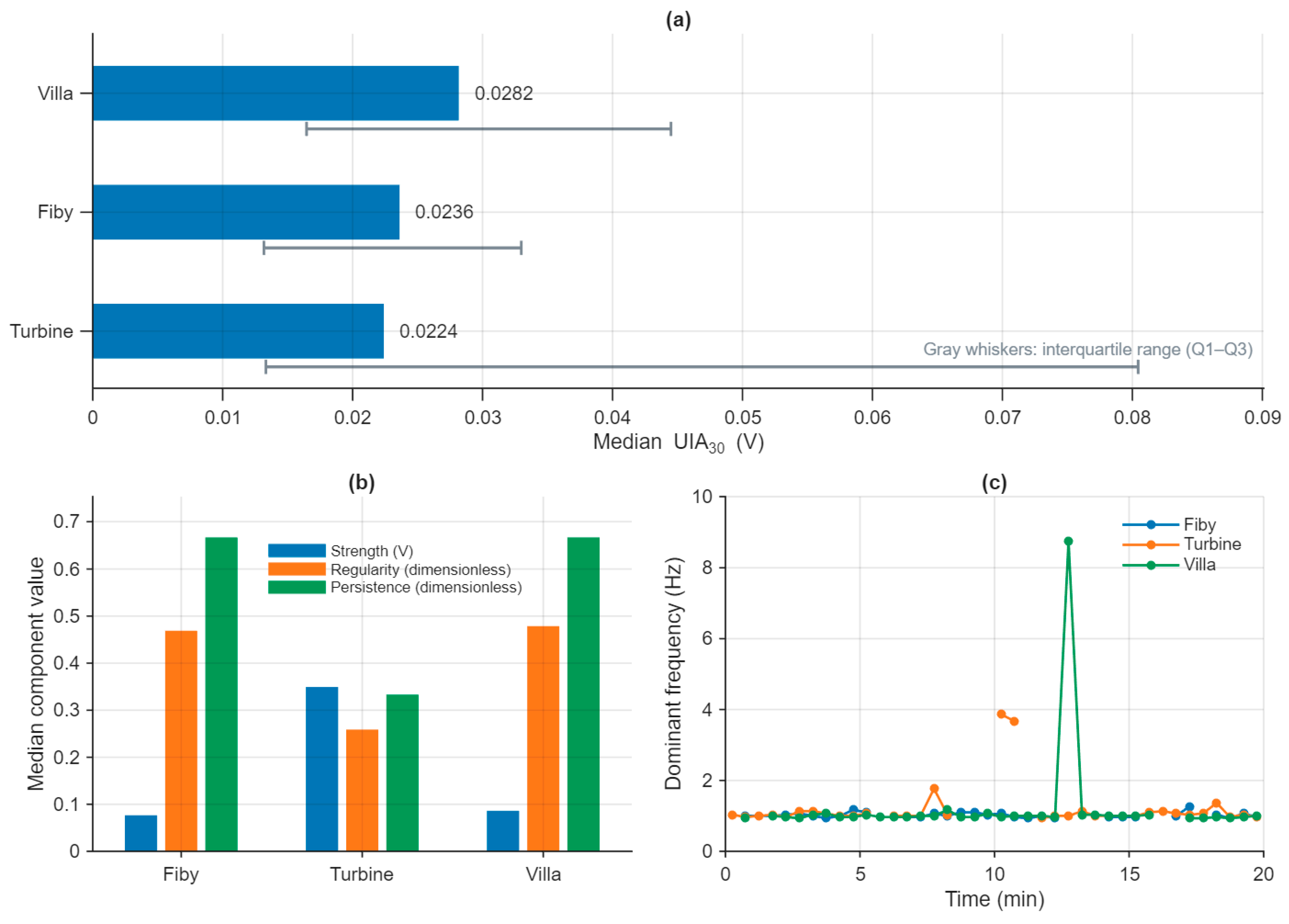
To evaluate the behavior of UIA under real measurement conditions, recordings from three contrasting environments were analyzed using the same processing parameters established in the preceding sections. The first recording (Fiby) was obtained at a reference location without a known local infrasound source. The second recording (Turbine) was acquired in the vicinity of a wind turbine and represents a measurement environment with a known strong infrasonic source. The third recording (Villa) was obtained inside a residential environment where persistent infrasonic activity had been observed, although its source was not identified. These three recordings were selected to examine how the individual UIA components distinguish between weak but persistent background activity, high-amplitude but less frequency-stable activity, and persistent activity of unknown origin.
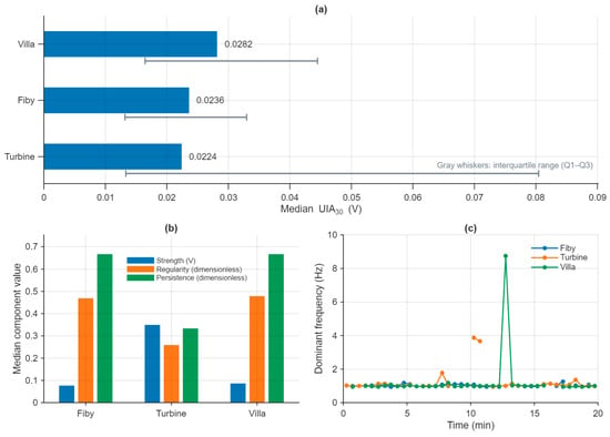
The three real-world recordings produced similar median UIA values but substantially different combinations of the underlying UIA components (Figure 5). Villa exhibited the highest median UIA (0.0282; IQR: 0.0165–0.0445), followed by Fiby (0.0236; IQR: 0.0132–0.0330) and Turbine (0.0224; IQR: 0.0133–0.0804). Notably, the comparatively large IQR observed for the Turbine recording indicates substantially greater window-to-window variability than for the other two environments.
Figure 5.
UIA analysis. (a) Median UIA calculated from accepted, non-overlapping 30 s analysis windows, with interquartile ranges (IQRs; 25th–75th percentiles). (b) Median values of the three UIA components: signal strength (S), spectral regularity (R), and temporal persistence (P). Signal strength and UIA are expressed in volts (V), whereas regularity and persistence are dimensionless. (c) Dominant frequency (Hz) as a function of recording time for the accepted 30 s windows.
Examination of the individual UIA components revealed markedly different signal characteristics despite the comparable median UIA values. Turbine showed the highest median Strength (0.349), approximately four times the values observed at Fiby (0.077) and Villa (0.086). However, its median Regularity (0.259) and Persistence (0.333) were substantially lower. Thus, the high signal magnitude at the turbine did not translate directly into a proportionally higher UIA because the spectral structure was less regular and less consistently recurrent.
In contrast, Fiby exhibited low Strength (0.077) but considerably higher Regularity (0.469) and Persistence (0.667), indicating a comparatively weak yet temporally persistent and spectrally structured background component. Villa showed a similar component pattern, with modest Strength (0.086) combined with high Regularity (0.479) and Persistence (0.667). This combination resulted in the highest median UIA among the three recordings despite a substantially lower signal magnitude than at the turbine.
The dominant-frequency analysis further distinguished the recordings. Fiby and Villa both exhibited a median dominant frequency of 1.00 Hz, whereas Turbine showed a slightly higher median of 1.017 Hz. More importantly, the window-level estimates demonstrate differences in temporal frequency behavior that are not represented by signal magnitude alone. This observation is consistent with the lower Regularity and Persistence obtained for the turbine recording.
These measurements illustrate an important property of the proposed metric: similar UIA values do not necessarily imply similar infrasonic signal characteristics. UIA results from the joint contributions of Strength, Regularity, and Persistence, allowing a strong but temporally variable signal to be distinguished from a weaker but highly persistent and regular signal. Consequently, the individual UIA components and dominant frequency should be reported together with the aggregate UIA value when characterizing real measurement environments.
3.5.2. Residential Case Study: Exploratory Spatial Measurements
A residential case study was conducted to investigate whether UIA could characterize spatial variations in infrasonic activity under real-world conditions. A total of 11 recordings were obtained, with one recording at each measurement location and no repeated measurement sessions. These included measurements inside a residence in which persistent low-frequency activity had been reported, immediately outside the residence, and at several surrounding locations, together with a recording from a geographically separate apartment used as a comparison location. To protect the privacy of residents and neighboring properties, geographical coordinates and identifying information are not reported.
Following the approximately 20 min instrument stabilization period described in Section 2.5, a continuous segment of the available signal was selected for analysis at each location. The analyzed segments were processed using the same predefined UIA procedure and parameter settings described in Section 2.1, Section 2.2 and Section 2.3, with independent, non-overlapping 30 s windows. For each recording, the median UIA and interquartile range were calculated, together with Strength, Regularity, Persistence, dominant frequency, and frequency stability. The case study was intended to characterize the spatial distribution and signal structure of the measured infrasonic activity, without drawing conclusions regarding physiological effects or causality.
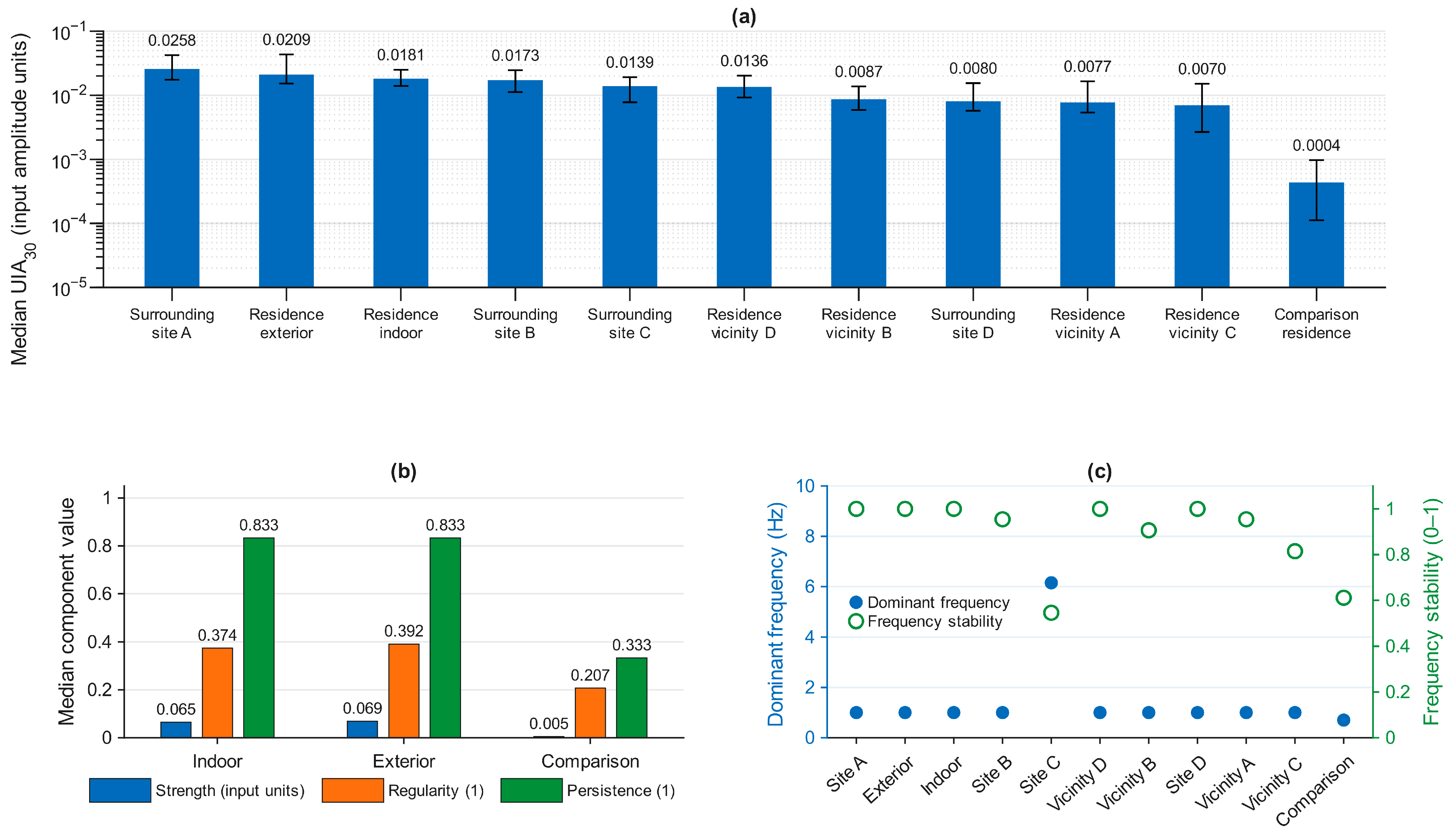
A marked difference in infrasonic activity was observed between the investigated residential environment and the geographically separate comparison residence. The indoor measurement at the investigated residence yielded a median UIA of 0.0181 (IQR: 0.0140–0.0251), while the measurement immediately outside the residence yielded a comparable median UIA of 0.0209 (IQR: 0.0152–0.0435). Both measurements exhibited a median dominant frequency of 1.00 Hz, a median Persistence of 0.833, and high frequency stability, indicating that the observed activity was not confined to an isolated short-duration event.
Measurements obtained at surrounding locations also frequently exhibited activity near 1 Hz, although the magnitude and temporal characteristics varied between sites. Median UIA ranged from approximately 0.0070 to 0.0258 across these measurements. Several locations showed a median dominant frequency of 1.00 Hz with high frequency stability, indicating that a component near 1 Hz was observed at multiple measurement positions in the surrounding environment.
In contrast, the comparison residence exhibited a median UIA of 0.00044 (IQR: 0.00011–0.00097), approximately 40 times smaller than the indoor median at the investigated residence. Strength was also substantially lower (0.0051 compared with 0.0651), and the dominant-frequency estimate shifted to approximately 0.70 Hz with lower frequency stability. Thus, application of the same analysis procedure to the two residential environments produced markedly different infrasonic activity profiles.
The spatial measurements revealed a recurring pattern of structured infrasonic activity within and around the investigated residence. The indoor recording yielded a median UIA of 0.0181, while the measurement immediately outside the residence yielded a comparable value of 0.0209. Several surrounding locations also exhibited elevated UIA values, ranging from approximately 0.007 to 0.026, whereas the geographically separate comparison residence showed a substantially lower median UIA of approximately 0.0004 (Figure 6a). The observed contrast therefore cannot be explained solely by whether the microphone was positioned indoors or outdoors.
Figure 6.
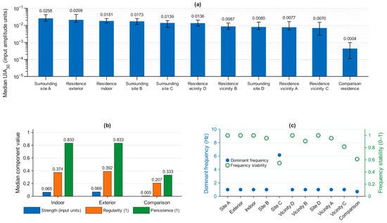
UIA results from the exploratory residential case study. (a) Median UIA calculated from accepted, non-overlapping 30 s analysis windows, with error bars indicating the interquartile range (IQR; 25th–75th percentiles). Recordings are arranged in descending order of median UIA, and numerical values are shown above the bars. (b) Median values of the three UIA components—signal strength (S), spectral regularity (R), and temporal persistence (P)—for the indoor, exterior, and comparison-residence recordings. Regularity and persistence are dimensionless, whereas strength retains the amplitude unit of the input signal. (c) Dominant frequency (left axis, Hz) and frequency stability (right axis, dimensionless) for all 11 recordings.
The component analysis further distinguished the two residential environments (Figure 6b). Measurements inside and immediately outside the investigated residence exhibited relatively low Strength but substantially higher Regularity and Persistence. In particular, median Persistence was approximately 0.83 at both locations. The comparison residence showed markedly lower Strength and Persistence, resulting in a substantially lower aggregate UIA. These findings illustrate that the elevated UIA observed at the investigated residence was associated primarily with recurring and structured activity rather than with high signal magnitude alone.
Dominant-frequency analysis provided additional evidence of spatially recurring signal structure (Figure 6c). A dominant component near 1 Hz was recovered at the investigated residence and at several surrounding measurement locations, generally with high frequency stability. However, not all locations exhibited the same spectral behavior; one surrounding measurement was dominated by a component near 6.15 Hz, and the comparison residence exhibited a different and less stable dominant-frequency pattern. Consequently, the measurements do not support attribution of all observed infrasonic activity to a single common source.
Taken together, the case study illustrates the application of UIA to a small set of real-world measurements exhibiting different infrasonic signal structures. A component near 1 Hz was observed at the investigated residence and at several surrounding measurement locations; however, the limited and uncontrolled sampling design does not permit statistical inference regarding its spatial prevalence or origin. The measurements were not designed for source localization, and potential environmental and measurement-related confounders cannot be excluded. The case study should therefore be interpreted as an exploratory demonstration of the descriptor rather than as independent validation of UIA or evidence of a spatially distributed common source. Furthermore, the measurements establish neither a causal relationship between the measured infrasonic activity and reported human responses nor a physiological threshold for such responses. These questions require larger, independently replicated measurement datasets and dedicated source-identification and controlled human-response studies.
Accordingly, independent field validation of UIA will require larger measurement campaigns conducted across multiple sites and source types, with predefined sampling protocols, repeated measurements, and independent replication. For applications involving spatial recurrence or source attribution, synchronized multi-location measurements, controlled-source experiments, and established source-localization methods would be required to distinguish source-related structure from environmental and meteorological variability. The present residential case study does not provide such validation and is therefore interpreted only as an exploratory application of UIA to measured field signals.
4. Conclusions
This study introduced Unit Infrasound Activity (UIA), a single-channel signal descriptor for characterizing structured infrasonic activity within the 0.5–10 Hz frequency range through the combined assessment of Strength, Regularity, and Persistence. Controlled synthetic-signal evaluation showed that UIA responds systematically to changes in signal magnitude, temporal presence, and frequency stability, while the reproducible Monte Carlo analysis demonstrated a monotonic association between median UIA and the predefined synthetic activity proxy and close agreement between imposed temporal presence and estimated Persistence. Dominant-frequency estimation was also accurate for the evaluated stable periodic signals.
The component-dependence and ablation analysis showed that Strength, Regularity, and Persistence are partially dependent rather than statistically independent quantities and that simpler component combinations emphasize different signal properties. The full multiplicative formulation is therefore not interpreted as an optimized detector or as the combination that maximizes association with any single signal characteristic. Instead, it provides a joint descriptor in which signal magnitude is weighted by spectral organization and temporal recurrence. The parameter-robustness analysis further showed that the principal synthetic-evaluation results were preserved under moderate one-at-a-time variation in the selected operational parameters, although temporal segmentation and frequency-tolerance settings influenced specific aspects of the metric.
Application to measured recordings illustrated that similar aggregate UIA values can arise from substantially different combinations of Strength, Regularity, and Persistence. The residential case study further demonstrated the use of UIA for describing differences among measurements obtained at multiple locations, including the observation of a component near 1 Hz at the investigated residence and at several surrounding measurement locations. However, the limited and uncontrolled field sampling does not permit inference regarding the spatial prevalence or origin of this component and does not constitute independent field validation of UIA. Source attribution, spatial generalization, and assessment of any relationship with human response require dedicated experimental designs and independently replicated measurements.
UIA should therefore be regarded as a complementary continuous descriptor of infrasonic signal structure rather than as a conventional sound-level measure, binary detector, source-identification method, or measure of human response. Its interpretation is strengthened by reporting the aggregate UIA together with Strength, Regularity, Persistence, dominant frequency, and statistical variability. Further work should evaluate the transferability of the operational parameters across different acquisition systems, source types, and measurement environments and establish the reproducibility of the metric in larger independent field datasets.
Supplementary Materials
The following supporting information can be downloaded at: https://www.mdpi.com/article/10.3390/signals7050101/s1, Supplementary Code S1: MATLAB code for reproducible generation and analysis of the 240 synthetic recordings.
Author Contributions
Conceptualization, K.T. and J.C.; methodology, K.T. and J.C.; software, K.T. and J.C.; validation, K.T. and J.C.; formal analysis, K.T. and J.C.; investigation, V.S.A.D. and J.C.; resources, K.T. and J.C.; data curation, V.S.A.D. and J.C.; writing—original draft preparation, K.T., J.C. and V.S.A.D.; writing—review and editing, K.T., V.S.A.D. and J.C.; visualization, K.T. and J.C.; supervision, K.T. and J.C.; project administration, K.T. and J.C. All authors have read and agreed to the published version of the manuscript.
Funding
This research received no external funding.
Data Availability Statement
The raw data supporting the conclusions of this article will be made available by the authors on request.
Acknowledgments
The authors acknowledge the valuable technical support of Mikael Sundberg.
Conflicts of Interest
The authors declare no conflicts of interest.
Abbreviations
The following abbreviations are used in this manuscript:
| IQR | Interquartile Range |
| MAD | Median Absolute Deviation |
| PSD | Power Spectral Density |
| UIA | Unit Infrasound Activity |
References
- Møller, H.; Pedersen, C.S. Hearing at Low and Infrasonic Frequencies. Noise Health 2004, 6, 37–57. [Google Scholar] [PubMed]
- Takahashi, Y.; Kanada, K.; Yonekawa, Y. The Relationship between Vibratory Sensation and Body Surface Vibration Induced by Low-Frequency Noise. J. Low Freq. Noise Vib. Act. Control 2002, 21, 87–100. [Google Scholar] [CrossRef] [Scilit]
- Tsunekawa, S.; Kajikawa, Y.; Nohara, S.; Ariizumi, M.; Okada, A. Study on the Perceptible Level for Infrasound. J. Sound Vib. 1987, 112, 15–22. [Google Scholar] [CrossRef] [Scilit]
- Ascone, L.; Uppenkamp, S.; Behler, O.; Lineton, B.; Burke, E.; Koch, C.; Kühn, S.; Geršak, G. Deductive Development and Validation of a Questionnaire to Assess Sensitivity to Very Low and Very High Frequency Sounds: SISUS-Q (Sensitivity to Infra-Sound and Ultra-Sound Questionnaire). Noise Health 2019, 21, 173–182. [Google Scholar] [PubMed]
- Baliatsas, C.; van Kamp, I.; van Poll, R.; Yzermans, J. Health Effects from Low-Frequency Noise and Infrasound in the General Population: Is It Time to Listen? A Systematic Review of Observational Studies. Sci. Total Environ. 2016, 557–558, 163–169. [Google Scholar] [CrossRef] [Scilit] [PubMed]
- Pawlaczyk-Luszczynska, M.; Szymczak, W.; Dudarewicz, A.; Śliwińska-Kowalska, M. Proposed Criteria for Assessing Low Frequency Noise Annoyance in Occupational Settings. Int. J. Occup. Med. Environ. Health 2006, 19, 185–197. [Google Scholar] [CrossRef] [Scilit] [PubMed]
- Jakobsen, J. Danish Guidelines on Environmental Low Frequency Noise, Infrasound and Vibration. J. Low Freq. Noise Vib. Act. Control 2001, 20, 141–148. [Google Scholar] [CrossRef] [Scilit]
- Holmberg, K.; Landstrom, U.; Söderberg, L.; Kjellberg, A.; Tesarz, M. Hygienic Assessment of Low Frequency Noise Annoyance in Working Environments. J. Low Freq. Noise Vib. Act. Control 1996, 15, 7–15. [Google Scholar] [CrossRef] [Scilit]
- Tombolato, A.; Bonomini, F.; Di Bella, A. Methodology for the Evaluation of Low-Frequency Environmental Noise: A Case-Study. Appl. Acoust. 2022, 187, 108517. [Google Scholar] [CrossRef] [Scilit]
- ISO 7196:1995; Acoustics—Frequency-Weighting Characteristic for Infrasound Measurements. International Organization for Standardization: Geneva, Switzerland, 1995.
- Bishop, J.W.; Fee, D.; Szuberla, C.A.L. Improved Infrasound Array Processing with Robust Estimators. Geophys. J. Int. 2020, 221, 2058–2074. [Google Scholar] [CrossRef] [Scilit]
- Ulivieri, G.; Ripepe, M.; Marchetti, E. Infrasound Reveals Transition to Oscillatory Discharge Regime during Lava Fountaining: Implication for Early Warning. Geophys. Res. Lett. 2013, 40, 3008–3013. [Google Scholar] [CrossRef] [Scilit]
- Ripepe, M.; Marchetti, E.; Delle Donne, D.; Genco, R.; Innocenti, L.; Lacanna, G.; Valade, S. Infrasonic Early Warning System for Explosive Eruptions. J. Geophys. Res. Solid Earth 2018, 123, 9570–9585. [Google Scholar] [CrossRef] [Scilit]
- Blom, P.; Bishop, J.W.; Green, D.N. Evaluation of Spectral Density-Based Clustering as a Means of Detection for Infrasound Transients on Single Channels. Geophys. J. Int. 2026, 246, ggag214. [Google Scholar] [CrossRef]
- Pásztor, M.; Czanik, C.; Bondár, I. A Single Array Approach for Infrasound Signal Discrimination from Quarry Blasts via Machine Learning. Remote Sens. 2023, 15, 1657. [Google Scholar] [CrossRef] [Scilit]
- Rousseeuw, P.J.; Croux, C. Alternatives to the Median Absolute Deviation. J. Am. Stat. Assoc. 1993, 88, 1273–1283. [Google Scholar] [CrossRef]
- Welch, P. The Use of Fast Fourier Transform for the Estimation of Power Spectra: A Method Based on Time Averaging over Short, Modified Periodograms. IEEE Trans. Audio Electroacoust. 1967, 15, 70–73. [Google Scholar] [CrossRef] [Scilit]

Disclaimer/Publisher’s Note: The statements, opinions and data contained in all publications are solely those of the individual author(s) and contributor(s) and not of MDPI and/or the editor(s). MDPI and/or the editor(s) disclaim responsibility for any injury to people or property resulting from any ideas, methods, instructions or products referred to in the content. |
© 2026 by the authors. Licensee MDPI, Basel, Switzerland. This article is an open access article distributed under the terms and conditions of the Creative Commons Attribution (CC BY) license.