A Coupled Acoustic-Poroelastic Approach to Model the Sound Transmission Loss Behavior of Nanoparticle-Fabric Composites

Abstract

Hybrid structural materials (HSMs), such as nanoparticle-treated fabrics, have been shown to enhance acoustic and ballistic performance in multifunctional protective structures. They offer a promising means for low-frequency (<~1000 Hz) noise mitigation, which remains a critical challenge in aerospace and defense applications. The measurement and modeling of their sound transmission loss (TL) behavior using a coupled acoustic–poroelastic approach is explored in this study. A colloid-based soaking and drying process is used to impregnate nanoparticles into the fabric. Previous studies using SEM imaging have established that at low (<~20 wt.%) treatment levels, the nanoparticles agglomerate in the interstitial spaces between yarn crossover points, whereas at higher levels, they begin to coat the yarn bundle tops. TL was measured experimentally using normal-incidence impedance tube tests. Further, parameters such as static flow resistivity, porosity, flexural modulus, and density required to model the neat and treat samples as fluid-filled porous solids using the Biot–Allard model were obtained from experiments for a limited set of neat and treated cases. Static flow resistivity was measured using an air permeability tester as per ISO 9237, and a modified version of the Peirce’s cantilever beam test was used to obtain the flexural modulus for neat and treated samples. Porosity was estimated using digital image analytics. The poroelastic fabric model was implemented in finite element simulations, and the predicted TL was compared with experiments including those for uncalibrated treated cases. The model shows close alignment with measured TL at low frequencies (<~600 Hz) for all cases but deviates closer towards the theoretical mass law at higher frequencies, where flanking effects and the influence of the hierarchy of pores are expected to be dominant in experiments. Further studies are underway to incorporate such higher-order effects to improve predictions at higher frequencies. The development of this model provides a means to capture the influence of nanoparticle addition on the acoustic performance of Kevlar, enabling fast and efficient virtual design iterations. The approach helps optimize HSMs for noise mitigation in multifunctional applications for the aerospace, defense, and infrastructural sectors.

1. Introduction

Noise pollution is a significant environmental concern, impacting human health and well-being through both auditory and non-auditory effects, including annoyance and stress [1,2]. Consequently, effective noise control is paramount in diverse settings, ranging from urban environments to specialized applications such as aerospace and defense [3,4]. Traditional noise mitigation strategies, which often rely on increasing material mass or thickness, present considerable drawbacks in weight-sensitive applications. This limitation has spurred intensive research into advanced materials and innovative acoustic solutions [5,6,7,8,9].

Porous materials, particularly fibrous absorbents, have long been recognized for their sound absorption capabilities [10,11,12,13]. The integration of advanced materials, such as hybrid structural materials (HSMs), offers a promising avenue for enhanced acoustic performance. Notably, nanoparticle-treated fabrics represent a cutting-edge class of HSMs that have demonstrated superior acoustic and ballistic properties, making them ideal for multifunctional protective structures [14,15,16,17]. Previous studies have, for instance, established that silica nanoparticle-impregnated Kevlar (SNK) fabrics deliver enhanced specific ballistic and stab resistance performance without compromising secondary functionalities [18,19]. This remarkable characteristic positions nanoparticle–fabric composites as a key enabler for lighter, more capable armors, thereby increasing useful payload across various application scenarios, including those in defense and infrastructure. The utility of nanoparticles extends beyond ballistic improvement; they have found diverse applications, from enhancing materials for thermal protection in space exploration [20] to pioneering breakthroughs in medical technology [21].

Beyond their structural and protective advantages, experimental characterization has demonstrated that the incorporation of nanoparticles into fabric structures, such as Kevlar, also leads to significant improvements in acoustic performance [22,23,24,25]. While neat, untreated woven Kevlar fabrics typically exhibit relatively low sound transmission loss, the addition of nanoparticles significantly improves this performance (+5 dB TL (2–6 kHz)). This acoustic enhancement is attributed to the modification of the material’s inherent porosity and the alteration of fluid flow characteristics within the fabric’s intricate structure, which directly influences sound transmission [22]. For example, the filling of pores by nanoparticles increases the static flow resistivity of the fabric, leading to better sound attenuation [24]. Therefore, extracting these localized microstructural changes to inform predictive macroscopic acoustic models is a critical step in advancing the material characterization of HSMs.

Given the intricate interplay between material properties and acoustic behavior, accurately predicting the sound transmission loss (TL) of these complex composite materials is crucial for their efficient design and optimization. While fully resolved 3D micro-mechanical finite element models may simulate these interactions from the nanoparticle to the yarn level with marginal improvement in predictions and their hierarchical contributions, they are computationally prohibitive for iterative engineering design. Therefore, there is a critical need for efficient, reduced-order predictive models. In this context, “reduced-order” refers to the homogenization of the multi-scale, discrete woven structure into an equivalent macroscopic poroelastic continuum. This approach subsumes the microscopic fluid–structure interactions into bulk effective parameters, eliminating the need to explicitly model nanoparticle-level details. Poroelasticity theory, which fundamentally describes the coupled interaction between solid deformation and fluid flow within a porous medium, provides an ideal framework for this purpose [26,27,28,29]. The Biot–Allard model, a widely accepted refinement of Biot’s theory, specifically accounts for viscous and thermal losses in fluid-saturated porous media, making it highly suitable for modeling the acoustic behavior of materials like SNK [28,29,30,31]. By establishing a reliable numerical model based on the Biot–Allard theory with the core assumptions that the inherently discrete, anisotropic woven composite can be effectively treated as a macroscopically isotropic and homogeneous porous medium under the small-strain acoustic loading conditions, and correlating it with targeted experimental data, it becomes a potential tool to simulate the acoustic performance of SNK fabric cases.

Hence, this study aims to develop and validate a numerical model for predicting the acoustic behavior of SNK fabrics. This involves establishing detailed experimental procedures to extract critical material properties of SNK, including airflow resistivity, equivalent out-of-plane bending stiffness modulus, and porosity. Airflow resistivity is determined using an air permeability tester, while the equivalent out-of-plane bending stiffness modulus is obtained through a modified fixed cantilever length flexibility test. Porosity is estimated using digital image analysis (DIA). These experimentally derived parameters are then integrated into a reduced-order numerical model based on the Biot–Allard poroelastic theory, implemented via finite element simulations. The model’s predictions for sound transmission loss are rigorously correlated with experimental results, including for uncalibrated treated cases, to validate its predictive capabilities. The ultimate goal is to provide a predictive tool that enables efficient virtual design iterations, offering significant advantages in terms of reduced development time and cost, and facilitating the rapid optimization of HSMs for diverse noise mitigation applications in the aerospace, defense, and infrastructural sectors.

2. Nanoparticle–Fabric Composites

In this study, the impregnation of Kevlar 29 Style 745 plain-woven fabric with 80 nm-diameter spherical silica nanoparticles was considered. The manufacturer-specified properties of the fabric and nanoparticle colloid are provided in Table 1 and Table 2.

Table 1. Manufacturer-specified properties of Kevlar K745 fabric.

Property	Value	Unit
Fiber type	29	-
Areal density	0.48	kg/m2
Fabric thickness	0.61	mm
Yarn set (Warp and Weft)	6.7	cm−1
Yarn titer	3000	denier
Number of filaments per yarn	1000	-

Table 2. Manufacturer-specified properties of Snowtex^® ST-ZL colloidal silica.

Property	Value	Unit
SiO2 concentration	40–41	wt.%
Na2O concentration	<0.07	wt.%
Particle shape	Spherical	-
Particle size	80–100	nm
Viscosity (at 25 °C)	<5	MPa.s
Specific gravity (at 25 °C)	1.29–1.32	-
pH	9.0–10.0	-
Appearance	Opalescent	-

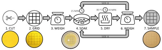
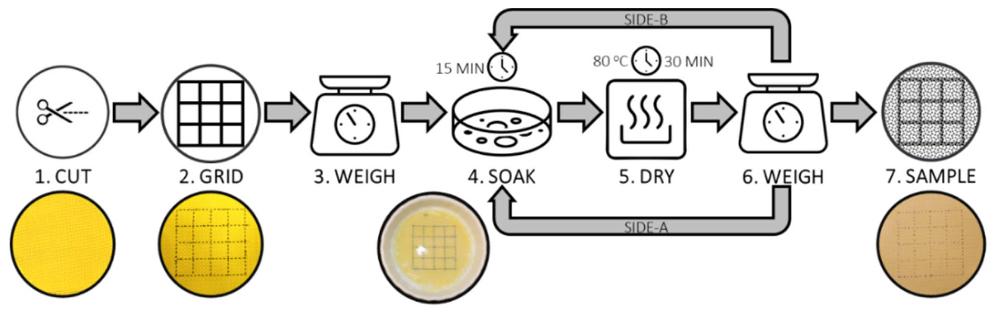
A manual soaking method [32] was used to impregnate nanoparticles to the Kevlar samples. The schematic representation of the process can be observed in Figure 1. The procedure was standardized to minimize variability between samples. Firstly, the neat fabric was cut into swatches of the required size (100 mm) from a dry bolt of fabric (Step-1) and subjected to an oven-drying procedure to remove any residual moisture. The grid lines were marked using a thin permanent marker along the yarn bundle tops such that a 4 × 4 grid was created with each grid enclosing 8 × 8 yarns in the warp and weft directions (Step-2). The cut and gridded swatch was weighed using a precision balance (Step-3). For a specific percentage by weight of nanoparticle addition, the aqueous colloid was measured and diluted with distilled water at a ratio of 1:4. A total liquid volume of ~12–15 mL per 100 mm × 100 mm sample area was prepared. The fabric swatch was soaked in half of this stabilized solution in a shallow dish for 15 min with one side (Side-A) facing up (Step-4). This process was repeated for Side-B to ensure uniform treatment for both sides. The fabric swatch was soaked in half of this solution in a shallow dish for 15 min with one side (Side-A) facing up (Step-4). The nanoparticles were allowed to infiltrate the yarn and fiber interstices under gravity. The swatch was then dried in a convection oven at 80 °C for 30 min to remove the moisture (Step-5). Once the moisture was removed, the swatch was weighed again to ascertain if the targeted percentage by weight of nanoparticle addition for one side was achieved (Step-6). If not, the process was repeated with the requisite amount of colloidal solution to make up for the weight addition needed for the side in question. Next, the soaking, drying, and weighing steps were undertaken for the other side (Side-B) of the swatch. Once the sample’s treated weight was within ±5% of the targeted total weight, the sample was stored in a zip lock bag until image acquisition (Step-7).

Figure 1. Steps involved in preparation of silica nanoparticle-impregnated Kevlar fabric samples using the soaking method.

3. Experimental Methods

3.1. Normal-Incidence Impedance Tube Test

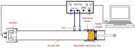
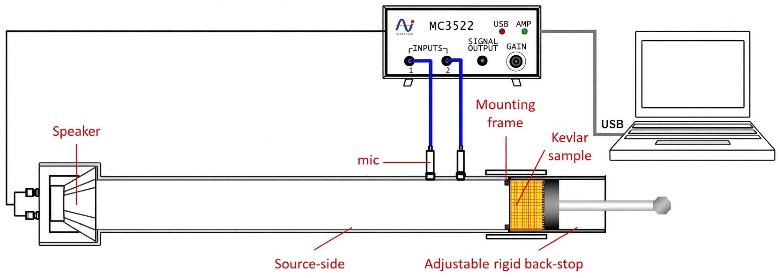
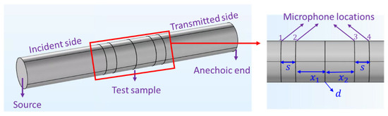
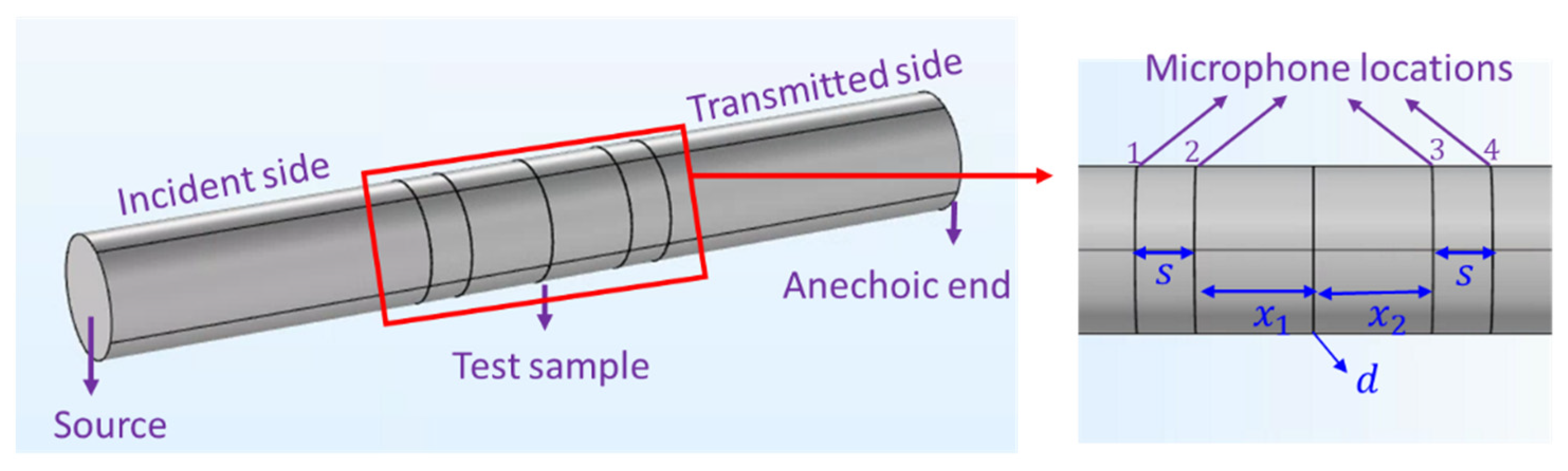
Experiments were conducted using a BSWA SW477 normal-incidence tube as per ASTM E2611 [33] for transmission loss (TL) measurement. The schematic representation for the experimental setup is shown in Figure 2. The Kevlar samples were assembled and mounted in the test section using a mounting frame. At least three trials were performed for each test case, and the average measurement was reported.

Figure 2. Schematic representation of the transmission loss experimental setup.

3.2. Air Permeability Test

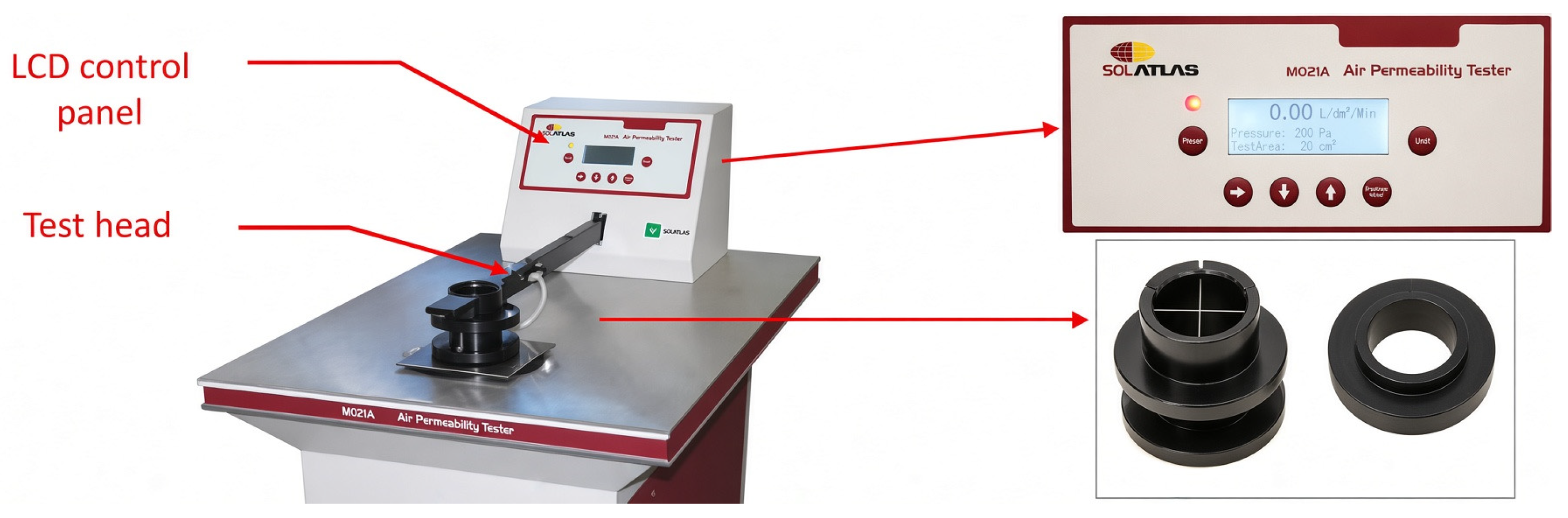
The determination of airflow resistivity can be achieved through air permeability measurements, following the guidelines outlined in ISO 9237 [34,35,36,37,38]. Figure 3 presents the air permeability test setup using an SDATLAS instrument.

Figure 3. Air permeability test setup.

The specific test conditions included a pressure range of 10 to 2500 Pa, a clamping force of 50 ± 5 N applied around the sample edge, and a test head radius of 50 mm. The relationship between airflow resistance and air permeability was obtained as follows:

$$R={\displaystyle \frac{\Delta p}{Q}}$$

(1)

where $\Delta p$ is the measured pressure difference in pascals and Q is the air permeability value obtained from the air permeability test. Consequently, the specific airflow resistance was then calculated as

$$R_s=R A_{cs}$$

(2)

where $d$ is the sample thickness and $A_{cs}$ is the cross-sectional area of the sample.

$$R_f={\displaystyle \frac{R_s}{d}}$$

(3)

3.3. Flexibility Test

A modified flexibility test known as the fixed cantilever length flexibility test was employed, as reported by Muhammad Bablu [19], to determine the flexural modulus of the Kevlar sample. In contrast to the ASTM D1338 [39] standard for flexibility testing, this modified approach prevents the dislodgement of the nanoparticles in the tested samples, thereby ensuring the accuracy of the obtained results.

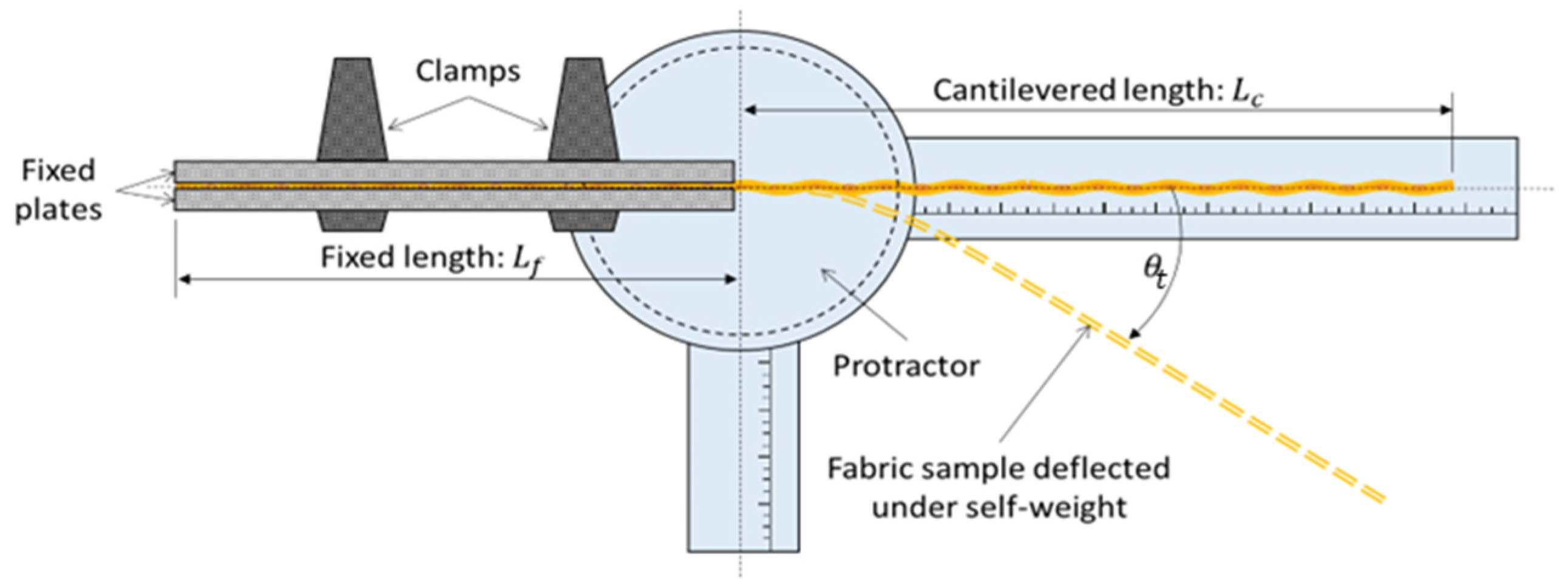
As depicted in Figure 4, neat Kevlar samples measuring 200 mm × 25 mm were employed for the test. A fixed length, ${\mathrm{L}}_{\mathrm{f}}$ = 70 mm, was clamped between two metal plates with a prescribed torque, leaving a cantilevered length, ${\mathrm{L}}_{\mathrm{c}}$ = 130 mm, free to flex under its self-weight. The warp yarn direction was aligned along the cantilevered length for consistency. A protractor equipped with a rotatable graduated scale was utilized to measure the tip deflection angle, ${\mathrm{\theta }}_{\mathrm{t}}$, while photographs captured the deflected shape of the fabric sample. By acquiring the coordinates of the deflected shape using Digital Image Analysis (DIA), correlation with mechanistic models facilitated the extraction of the flexural rigidity of the sample. Subsequently, flexural rigidity was employed to compute the flexural modulus of the Kevlar samples. A total of nine data sets were collected, comprising three samples of neat, 20 wt.%, and 40 wt.% SNK with three trials performed for each sample.

Figure 4. Schematic depiction of the experimental setup for the flexibility test.

3.4. Porosity Test

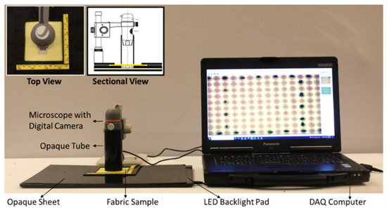
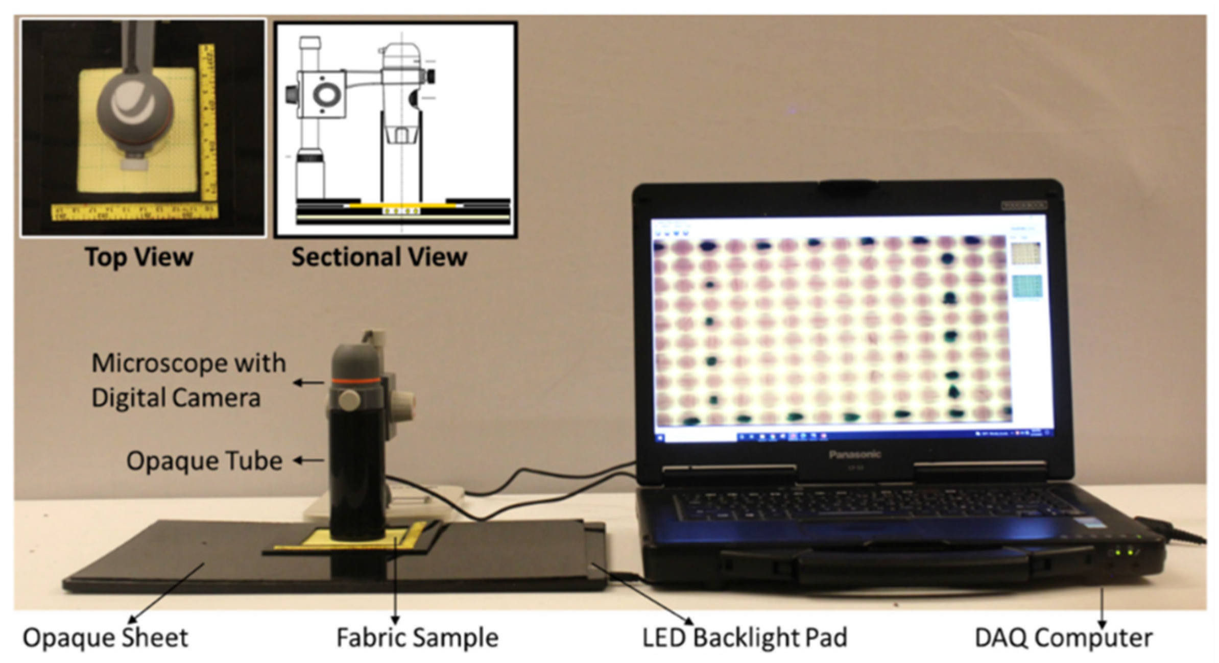
An estimate value for the porosity (specifically quantified in this study as the optical open area fraction) was obtained using the digital image acquisition system consisting of a 15 MP digital camera coupled to a microscope that was focused on to the fabric samples through the confines of an opaque tube, as presented in Figure 5. The sample itself was illuminated using an LED backlight sandwiched between opaque plastic panels such that the light passed only though the sample under evaluation. The LED’s white light was set to a brightness of 7000 Lux through this study to ensure sufficient light transmission without saturating the interstitial spaces or shifting the greyscale value spectrum excessively toward the brighter region, which would reduce the ability to discern changes in resolution. A study was conducted to determine optimal camera settings, resulting in the selection of ISO 800, a shutter speed of 1/100 s, and an aperture setting of f/5.6 [32], as these provided a balanced brightness amplification with clear distinction in features between neat and treated fabrics without excessive saturation or loss of surrounding area visibility.

Figure 5. Experimental setup for DIA data acquisition.

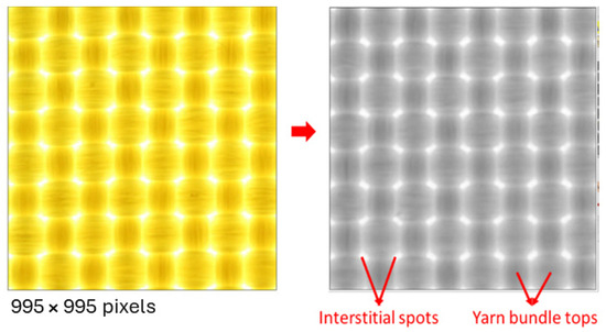
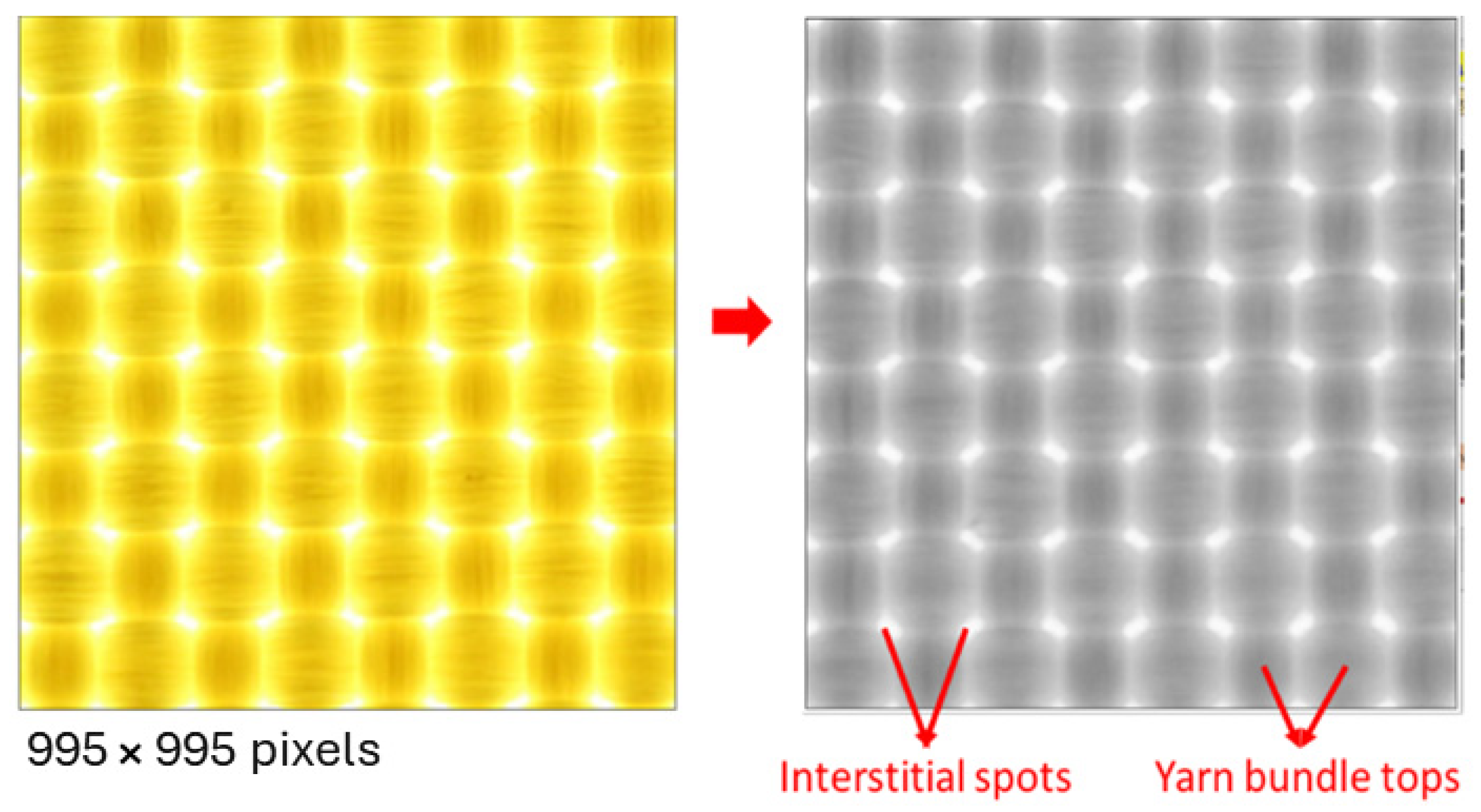
The orientation of warp and weft directions was kept unaltered for all samples during image capture. Weft is horizontal and warp is vertical in the images. All external light sources were extinguished during data acquisition in order to avoid non-source illumination of the sample. Images captured on Figure 5, contained up to four grids, and were cropped to a single grid excluding grid lines for analysis, yielding a resolution of 995 × 995 pixels and a file size of 80.6 kB, which provided sufficient detail for evaluating fabric impregnation quality. The acquired images, originally in RGB color, were converted to 8-bit greyscale using a weighted average of RGB channels. These 8-bit greyscale images were then cataloged with sample and grid identifiers and stored on a DAQ computer for further processing. Grey Scale Value (GSV) histograms were generated by counting the occurrence of each pixel value (0–255) within each grid square.

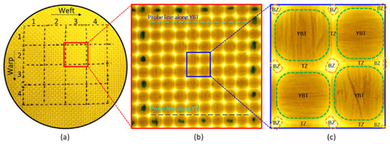
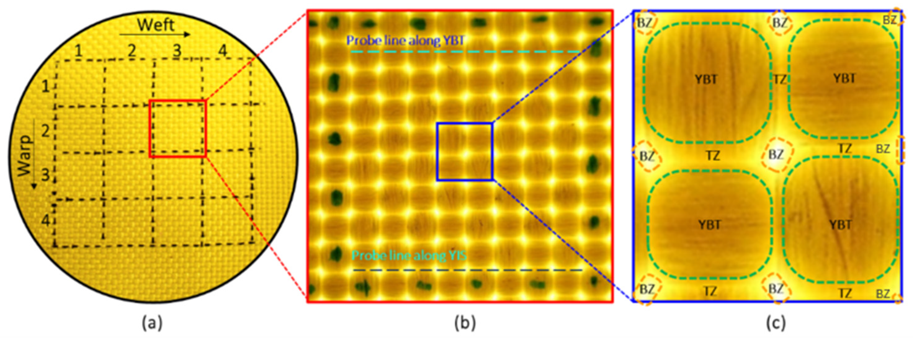
The hierarchy of fabric regions for digital image analytics is shown in Figure 6. Each sample consisted of 4 × 4 grids on each side with each grid containing 8 × 8 yarns in the warp and the weft direction. As shown in the zoomed view within a grid, at each yarn crossover point, the image can be divided into three different zones—(i) The Yarn Bundle Tops (YBT), (ii) the Brightest Zones (BZ) corresponding to Yarn Interstitial Spaces (YIS), and (iii) Transition Zone between YBT and the YIS based on the amount of backlight that passes through the sample.

Figure 6. Hierarchical regions for DIA data extraction: (a) fabric sample with grid markings; (b) digital image acquired for a selected grid showing probe line examples along Yarn Bundle Tops (YBT) and Yarn Interstitial Spaces (YIS); (c) zoomed view of a selected set of yarn crossover points with YBT, showing the Brightest Zones (BZ) corresponding to YIS and the demarcated Transition Zones (TZ).

4. Modeling

4.1. Theoretical Background

4.1.1. Poroelastic Material Model

Poroelasticity describes the interaction between solid deformation and fluid flow within a porous medium. When an external force acts upon a porous material, the fluid in the pores undergoes pressure changes under mechanical stress, inducing fluid movement. This alteration in pore volume leads to elastic deformation of the material [28]. Nanoparticles impregnated in fabric present a scenario where the poroelastic model could be applied, because fabric themselves are porous. The addition of nanoparticle affects the porosity and passage of fluid through the pores in the fabric.

Modeling poroelasticity requires coupling two phenomena: firstly, the fluid velocity’s proportionality to pressure difference over distance governed by Darcy’s law [40], and secondly, the structural displacement of the porous matrix, as described by Biot poroelasticity [27]. The acoustic behavior of porous materials has been extensively studied, ranging from empirical equivalent fluid models to more sophisticated approaches like the Biot theory and semi-empirical models, developed to accurately depict wave propagation in porous media [28,41]. Essentially, Biot extended the classical theory of linear elasticity to porous media saturated with fluids [30,31]. The effectiveness of these models hinges on material property parameters. The more the parameters of the model, the more accurately and in greater detail the behavior can be explained. HSMs, being porous due to the manufacturing process, are generally anisotropic and inhomogeneous [42]. However, for computational simplicity and parametric simplification, assuming isotropy and homogeneity of the porous material may suffice to replicate experimental results.

The model describes wave propagation in porous media, which can be applied to HSMs, based on viscous and thermal loss theorems [30,31]. The coupling of the acoustic and poroelastic media can be implemented in COMSOL 53a, to obtain a numerical simulation of the theoretical model. This interface integrates pressure acoustics, frequency domain, and poroelastic waves, along with the Acoustic–Porous Boundary Multiphysics coupling feature. The pressure acoustic implemented in the frequency domain interface computes pressure variations to model the propagation of acoustic waves in fluids under steady-state conditions [28,43,44,45,46,47].

Consider Biot’s expression for poroelastic waves [27,48]:

$${\rho }_{av}{\displaystyle \frac{{\partial }^2}{\partial t^2}}{x}_p+{\rho }_f{\displaystyle \frac{{\partial }^2}{\partial t^2}}{x}_f-\nabla \mathrm{\sigma }=0$$

(4)

$${\rho }_f{\displaystyle \frac{{\partial }^2{x}_p}{\partial t^2}}+{\displaystyle \frac{{\eta }_f}{\kappa }}{\displaystyle \frac{\partial x_f}{\partial t}}+{\displaystyle \frac{\mathrm{{\rm Y}}}{{\epsilon }_p}}{\rho }_f{\displaystyle \frac{{\partial }^2{x}_f}{\partial t^2}}-\nabla p_f=0$$

(5)

where $x_p$ is the displacement of the porous material, $\varrho$ is the total stress tensor (fluid and porous material), $x_f$ is the fluid displacement, ${\rho }_f$ is the fluid density, ${\eta }_f$ is the static fluid viscosity, $\mathrm{{\rm Y}}$ is the tortuosity, ${\epsilon }_p$ is the porosity, $p_f$ is the fluid pore pressure, $\kappa$ is the permeability, ${\rho }_{av}={\rho }_d+{ϵ}_p{\rho }_f,$ and ${\rho }_d$ is the material density. These equations represent the conservation of momentum for the solid phase and fluid phase. Assuming a time harmonic dependent variable, $x_p \left(x,t\right)=x_p\left(x\right)e^{i\omega t}, x_f\left(x,t\right)=x_f\left(x\right)e^{i\omega t}$, Biot’s expressions become the following:

$$-{\rho }_{av}{\omega }^2{x}_p+{\rho }_f{\omega }^2{x}_f-\nabla \mathrm{\sigma }=0$$

(6)

$$-{\rho }_f{\omega }^2{x}_p-{\omega }^2{\rho }_c\left(\omega \right)x_f+\nabla p_f=0$$

(7)

where the complex density is given as

$${\rho }_c\left(\omega \right)={\displaystyle \frac{\mathrm{{\rm Y}}}{{\epsilon }_p}}{\rho }_f+{\displaystyle \frac{{\eta }_f}{i\omega \kappa }}$$

(8)

The displacement-based formulation, involving $x_p$ and $x_f$, is not optimal from the numerical perspective since it needs to solve for two displacement fields [28,44,45]. The poroelastic waves interface computes for the fluid pore pressure variable, $p_f$, instead of the fluid displacement field, $x_f$. Eliminating the displacement, $x_f,$ the total stress tensor is divided into contributions from the elastic porous matrix and the pore field:

$$\varrho \left(x_p,p_f\right)={\varrho }_d\left(x_p\right)-{\alpha }_B{p}_{f}I$$

(9)

where the identity tensor, $I$, means that the pore pressure contributes to the diagonal of the total stress tensor, $\varrho$; ${\alpha }_B$ is the Biot–Willis coefficient; ${\varrho }_d$ is the elastic stress tensor. Biot’s wave equations can be written in terms of displacement, $x_p$, and pore pressure, $p_f$ as

$$-{\omega }^2\left({\rho }_{av}-{\displaystyle \frac{{\rho }_f^2}{{\rho }_c\left(\omega \right)}}\right)x_p-\nabla ·\left({\varrho }_d\left(x_p\right)-{\alpha }_B{p}_{f}I\right)=-{\displaystyle \frac{{\rho }_f}{{\rho }_c\left(\omega \right)}}\nabla ·p_f$$

(10)

$$-{\displaystyle \frac{{\omega }^2}{K}}{p}_f-\nabla ·\left({\displaystyle \frac{1}{{\rho }_c\left(\omega \right)}}\left(\nabla ·p_f-{\omega }^2{\rho }_f{x}_p\right)\right)={\omega }^2{\alpha }_B\nabla ·x_p$$

(11)

The Biot modulus, $M$, is computed from porosity, ${\epsilon }_p$, fluid compressibility, ${\chi }_f$, the Biot–Willis coefficient, ${\alpha }_B$, and the bulk modulus of the porous matrix, $K_d$, as

$${\displaystyle \frac{1}{M}}={\epsilon }_p{\chi }_f+({\alpha }_B-{\epsilon }_p)\left(1-{\alpha }_B\right)/K_d$$

(12)

In Equations (10) and (11), the viscous and thermal losses are not considered. To include the losses, the static value of the viscosity and fluid compressibility in Equations (8) and (12), respectively, are replaced by their frequency dependent expressions [28], as described in Equations (13) and (14), respectively.

The frequency-dependent complex viscosity is given by

$$\eta \left(\omega \right)={\eta }_f{\left(1+{\displaystyle \frac{4i\omega {\mathrm{{\rm Y}}}^2{\eta }_f{\rho }_f}{R_f^2{L}_v^2{\epsilon }_p^2}}\right)}^{{\displaystyle \frac{1}{2}}}$$

(13)

where $L_v$ is the viscous characteristic length, $R_f$ is the flow resistivity, $P_r$ is the Prandtl number, and $p_A$ is the ambient pressure.

The frequency-dependent complex fluid compressibility is given by

$${\chi }_f\left(\omega \right)={\displaystyle \frac{{\epsilon }_p}{\gamma p_A}}\left[\gamma -\left(\gamma -1\right){\left(1+{\displaystyle \frac{8{\eta }_f}{i\omega L_{th}^2{P}_r{\rho }_f}}\sqrt{1+{\displaystyle \frac{i\omega L_{th}^2{P}_r{\rho }_f}{16{\eta }_f}}}\right)}^{-1}\right]$$

(14)

with

$$\mathrm{{\rm Y}}=1+2{\displaystyle \frac{\mathrm{ϵ}}{\mathrm{d}}}$$

(15)

$$ϵ=\left(1-1.13\xi -0.09{\xi }^2+0.27{\xi }^3\right) 8L_{ch}/3\pi$$

(16)

where $\gamma$ is the specific heat ratio, $L_{th}$ is the thermal characteristic length, $P_r$ is the Prandtl number, and $p_A$ is the quiescent pressure.

The value $\xi =2\sqrt{{\epsilon }_p/\pi }$, and $L_{ch}$ is the characteristic length. For a material that has identical and parallel rectangular perforations and cross-sectional areas, the characteristic length is given by [28]

$$L_{ch}=1.2 \sqrt{{\displaystyle \frac{12{\eta }_f}{R_f{\epsilon }_p}}}$$

(17)

where ${\eta }_f$ is the dynamic viscosity of air and $R_f$ is the flow resistivity.

4.1.2. Estimation of Parameters

To model a poroelastic material using Biot’s poroelastic wave equations (Equations (10) and (11)), the following parameters were required: material density, fluid density, fluid bulk modulus, porosity, tortuosity, Prandtl number, Biot–Willis coefficient, Young’s modulus (embedded in the stress tensor), static fluid viscosity, thermal and viscous characteristic lengths, ambient pressure, and specific heat ratio. The fluid parameters are known, but due to the intricacy of the neat and treated Kevlar samples, obtaining the material properties posed significant challenges. Ensuring the accuracy and validation of these parameters is crucial for precise model results. While fiber-level values for some parameters of neat Kevlar are typically available from the manufacturer, fabric-level properties are not readily available. To achieve comprehensive validation of experimental data with the model, testing conditions were devised to obtain the required material properties, regardless of sample complexity. The material properties measured were density, porosity, airflow resistivity, and the Young’s modulus.

Because the optical method primarily captures the macro-porosity of the interstitial spaces, which is the major contributor among the hierarchy of pores in the treated fabrics. Therefore, the Biot–Allard model was applied in a phenomenological manner in this approach. Consequently, the inferred parameters, including tortuosity and the thermal and viscous characteristic lengths, were treated as empirical fitting parameters derived from macro-porosity rather than as exact physical micro-geometric properties. The test summary for measured parameter estimation is shown in Table 3.

Table 3. Summary of neat and treated Kevlar’s parameters estimated from experiments.

Case #	Test Type	Nanoparticle	Treated (wt.%)
Neat	Static flow resistivity (SFR) Young’s modulus (E) Porosity (εp) $\mathrm{Density} ({\rho }_d)$	—	—
SiO2_80 nm		Silica	20, 40

4.2. Finite Element Model

The FEM simulation model of the NIT with a circular cross-section for the porous material is presented. A numerical model for poroelastic materials utilizing COMSOL was calibrated, offering a platform to simulate complex porous materials.

The FEM simulation of the NIT closely mirrors the experimental testing conditions. Typically, an NIT tube consisted of two tube sections: an incident tube and a transmitted-side tube, both sharing the same circular internal cross-sectional area. The test sample was placed between these tubes, with a pair of microphones strategically positioned on either side. Figure 7 illustrates a detailed schematic of a typical setup. The frequency range of the test was contingent upon the tube’s dimensions listed in the table, the microphone spacing, and the speed of sound in air. The setup depicted covered a frequency from 250 to 1600 Hz.

Figure 7. Views of the FEM simulation model of the NIT with a circular cross-section.

The tube’s length ensured the complete development of plane wave propagation conditions before reaching the microphones and the barrier. The source was excited with an input sound pressure, and the sound was transmitted through the barrier, where absorption, reflection, and transmission occurred. Four microphones recorded the complex sound pressure at designated locations within the tube. At the far end of the transmitted side, two different BCs were set for the single- and double-load methods. The single-load method utilized an anechoic termination, preferable for geometrically symmetric barriers, whereas the double-load method, employed for asymmetric samples, incorporated two different terminations (anechoic and open/closed).

The ASTM E2611 standard [33] for NIT and the experimental setup’s features served as guides for the model’s implementation. An acoustic–poroelastic wave interaction analysis, in the frequency domain, was conducted for the frequency range of interest. An input pressure signal was applied at the incident port, propagating through the tube. Since an infinite impedance BC implies a rigid duct wall, the air column in the tubes was modeled with BCs of infinite impedance. A plane wave radiation BC was applied at the transmitted-side far end, representing an anechoic termination. The dimensions of the tube, as specified in Table 4, and the microphone locations were chosen based on the upper and lower frequency limits of interest for testing. Once the complex pressure values at the four microphone locations were extracted from the simulation, then the TL for the barrier test sample can be calculated [33,49] as

$$TL=20{\log }_{10}\left|{\displaystyle \frac{1}{t_0}}\right|$$

(18)

Table 4. Dimensions of the circular-cross-section NIT for TL measurement.

Geometric Parameter	Value (mm)
Length of each half of the tube	745
Tube radius (air column)	50
Kevlar sample thickness (d)	0.61
Spacing between microphones $\left(s\right)$	70
Distance between the sample incidence surface and mic 2 ($x_1)$	175
Distance between the sample incidence surface and mic 3 ($x_2)$	175

The transmission coefficient ($t_0$) is given as

$$t_0={\displaystyle \frac{2e^{i\omega d}}{T_{11}+\frac{T_{12}}{{\rho }_0{c}_0}+{\rho }_0{c}_0{T}_{21}+T_{22}}}$$

(19)

The transfer matrix is given as

$$\left[\begin{array}{cc}{T}_{11}& T_{12}\\ T_{21}& T_{22}\end{array}\right]=\left[\begin{array}{cc}{\displaystyle \frac{p_d{v}_d-p_0{v}_0}{p_0{v}_d-p_{d}u{v}_0}}& {\displaystyle \frac{p_0^2-p_d^2}{p_0{u}_d-p_d{v}_0}}\\ {\displaystyle \frac{v_0^2-v_d^2}{p_0{v}_d-p_d{v}_0}}& {\displaystyle \frac{p_d{v}_d-p_0{v}_0}{p_0{v}_d-p_d{v}_0}}\end{array}\right]$$

(20)

where the acoustic pressure and particle velocity on both faces of the sample are given as

$$p_0=A+B$$

(21)

$$v_0={\displaystyle \frac{A-B}{{\rho }_0{c}_0}}$$

(22)

$$p_d=C{e}^{-i\tilde{v}d}+D{e}^{i\tilde{v}d}$$

(23)

$$v_d={\displaystyle \frac{C{e}^{-i\tilde{v}d}-D{e}^{i\tilde{v}d}}{{\rho }_0{c}_0}}$$

(24)

The forward and backward travelling waves on either side of the sample are given as

$$A=i {\displaystyle \frac{p_1{e}^{-i\tilde{v}{x}_1}-p_2{e}^{-i\tilde{v}(x_1+s)}}{2\sin \left(\tilde{v}s\right)}}$$

(25)

$$B=i {\displaystyle \frac{p_2{e}^{i\tilde{v}\left(x_1+s\right)}-p_1{e}^{i\tilde{v}{x}_1}}{2\sin \left(\tilde{v}s\right)}}$$

(26)

$$C=i {\displaystyle \frac{p_3{e}^{i\tilde{v}\left(x_2+s\right)}-p_4{e}^{i\tilde{v}{x}_2}}{2\sin \left(\tilde{v}s\right)}}$$

(27)

$$D=i {\displaystyle \frac{p_4{e}^{-i\tilde{v}{x}_2}-p_3{e}^{-i\tilde{v}(x_2+s)}}{2\sin \left(\tilde{v}s\right)}}$$

(28)

where $\omega$ is the excitation frequency, ${\rho }_0$ is the air density, $s$ is the spacing between microphones, $c_0$ is the speed of sound in air, $\tilde{v}$ is the wave number, $\omega /c_0$, and the $p_1, p_2, p_3, p_4$ are the complex pressures extracted from the simulation.

5. Discussion of Results

5.1. Static Flow Resistivity

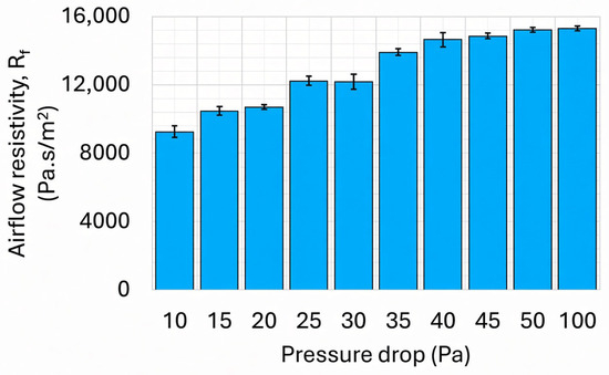
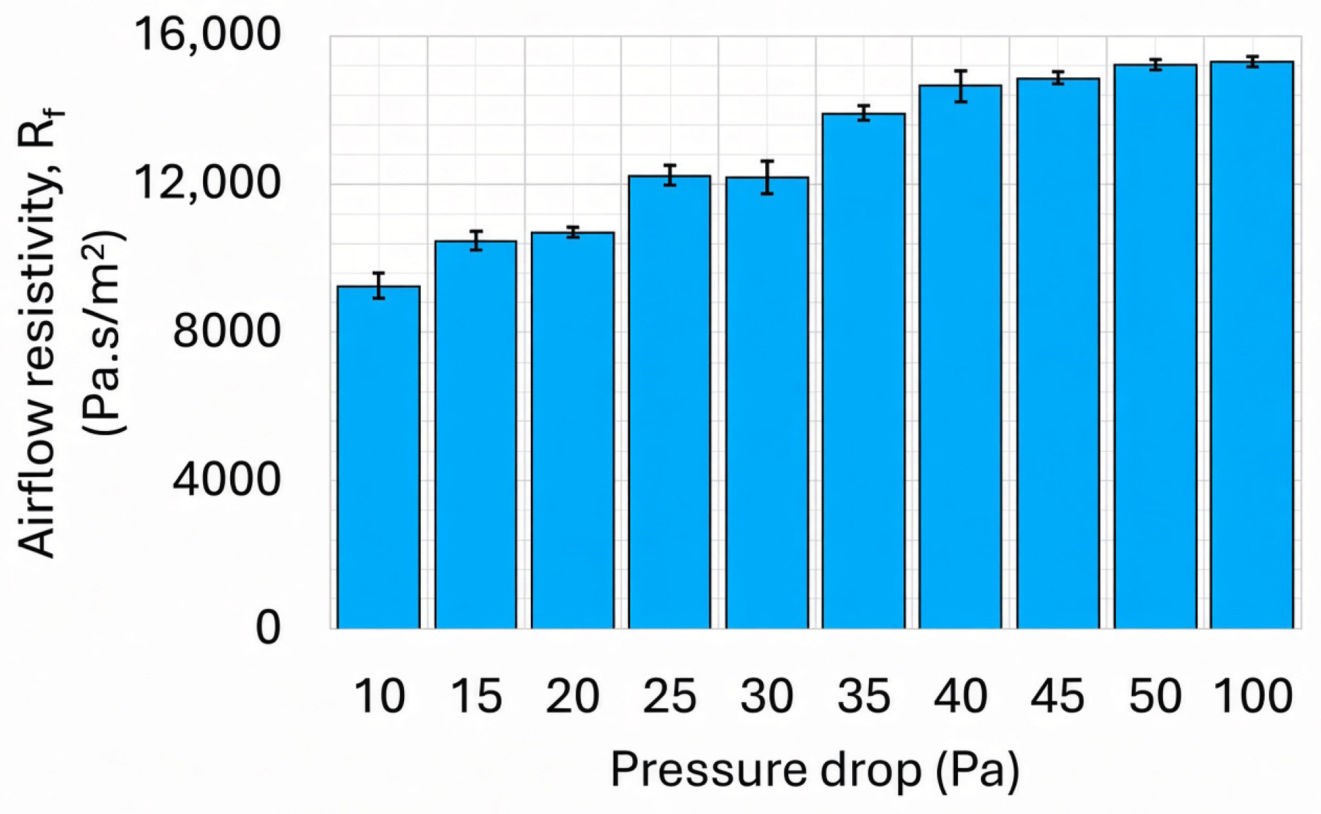
To verify the air permeability method for determining flow resistivity, a melamine foam with a measured density of approximately 7.07 kg/m³ was tested. Figure 8 presents the flow resistivity values estimated from air permeability measurements conducted at varying pressure drops with three trials.

Figure 8. Measured airflow resistivity at various pressure drops using an air permeability tester for melamine foam.

The airflow resistivity measured at a pressure drop of 10 Pa was found to be 9300 Pa.s/m². The obtained values comparatively align with the SFR reported for melamine foam by Tao et al. [50], which was 10,500 Pa.s/m² for a melamine foam with a density of 9 (±1.5) kg/m³.

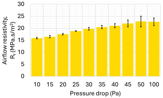
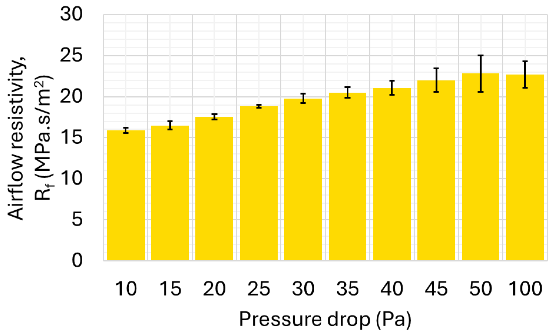
The flow resistivity of neat Kevlar was then determined using air permeability measurements conducted at varying pressure drops, with three trials performed for each pressure level. The results are shown in Figure 9. The airflow resistivity of neat Kevlar was estimated as 15.89 MPa.s/m².

Figure 9. Measured airflow resistivity at various pressure drops using an air permeability tester for neat Kevlar.

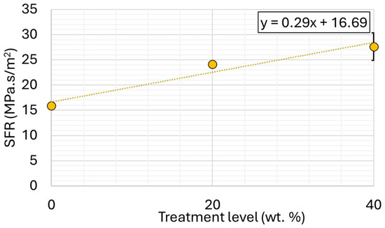
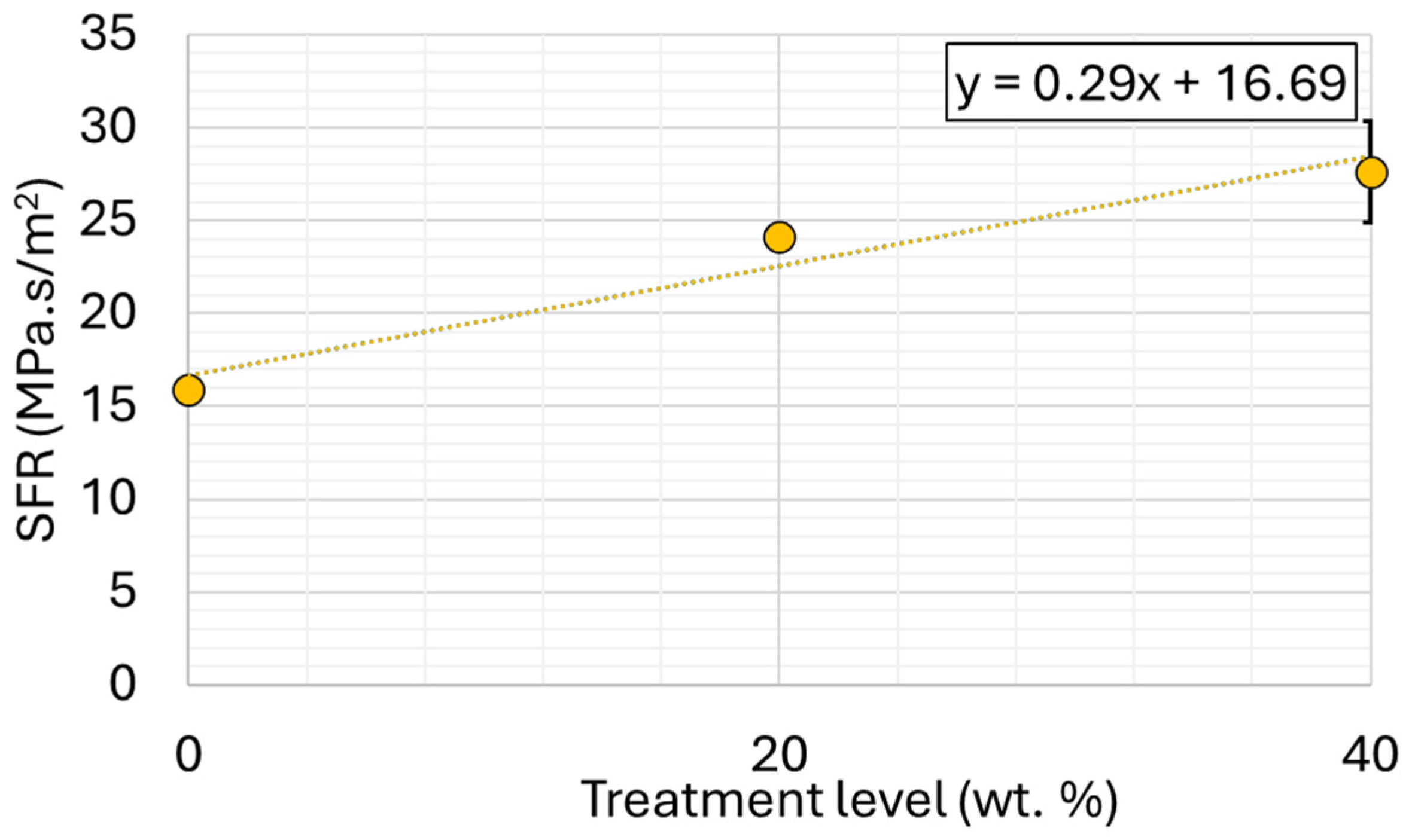
The same approach was applied to estimate the airflow resistivity of nanoparticle-impregnated Kevlar samples. The evolution of static flow resistivity (SFR) as a function of various treatment levels in 80 nm SNK is shown in Figure 10. The SFR increased linearly from 15.89 MPa.s/m² for neat Kevlar to 27.6 MPa.s/m² for 40 wt.% SNK with increasing silica nanoparticle treatment. This observed increase in SFR can be attributed to the filling of pores within the Kevlar fabric by the added nanoparticles. The SFR obtained from the experimental measurements was incorporated into the simulation model to predict the TL characteristics of Kevlar samples with varying nanoparticles treatment levels. In addition, a linear regression analysis was performed on the experimental data to extract SFR for new cases. These extrapolated parameters were then be used as inputs for the simulation model to predict the TL of these new cases, thereby validating the model’s predictive capability for nanoparticle-treated Kevlar.

Figure 10. Static airflow resistivity for neat, 20 wt.%, and 40 wt.% SNK fabrics.

5.2. Equivalent Out-of-Plane Bending Stiffness Modulus

The term “modulus” is commonly used to quantify a material’s response to deformation under external forces, with various types of moduli associated with different materials. Nanoparticle-impregnated Kevlar is typically porous and exhibits anisotropic and inhomogeneous properties. Inhomogeneous materials like Kevlar fabric have different moduli in various directions. The in-plane tensile moduli, although different, are quite high and nonlinear [18]. The moduli in compression and tension are quite different. However, to simplify computation and parameterization, assuming isotropy and homogeneity of the porous material may be sufficient to replicate experimental results. Moreover, in the modeled normal incidence transmission (NIT) testing conditions, sound waves strike the sample surface at a normal angle, inducing primarily out-of-plane deformation. Consequently, in-plane deformation is negligible. Given the small deformation induced by acoustic loading, the anisotropic behavior of the Kevlar fabric is unlikely to be significant. Prior studies indicate that in-plane loading results in a low modulus response under small deformations [18]. Therefore, in the regime of small acoustic-induced deformation, the Kevlar samples can be modeled using an isotropic modulus, simplifying the analysis. It is important to acknowledge that treated woven fabrics are inherently composed of discrete hierarchical sub-structures. Therefore, the parameter utilized in this model acts as an “equivalent out-of-plane bending stiffness modulus” that lumps together the complex micro-kinematics of the fabric, including individual yarn bending, inter-yarn shear, and frictional effects. Specifically, when nanoparticles impregnate the fabric and agglomerate, they induce mechanical interlocking between the yarns. Under small acoustic deformation, overcoming these frictional effects due to the mechanical interlockings leads to enhanced energy dissipation. By utilizing this equivalent modulus, all of these discrete, micro-mechanical frictional interactions are subsumed into a single macroscopic parameter appropriate for the small-strain, out-of-plane acoustic loading characteristic of the NIT experiments. Since the deformation in NIT testing occurs in the bending direction, the out-of-plane deformation is also small in this regime, the relevant modulus for this phenomenon can be termed the “effective modulus”. This equivalent out-of-plane bending stiffness modulus, representing the modulus that governs the out-of-plane deformation response of the sample under small strain conditions, is determined by measuring the flexural modulus through a flexibility test, providing a practical approach for acoustic modeling.

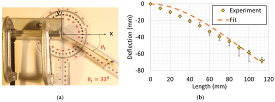
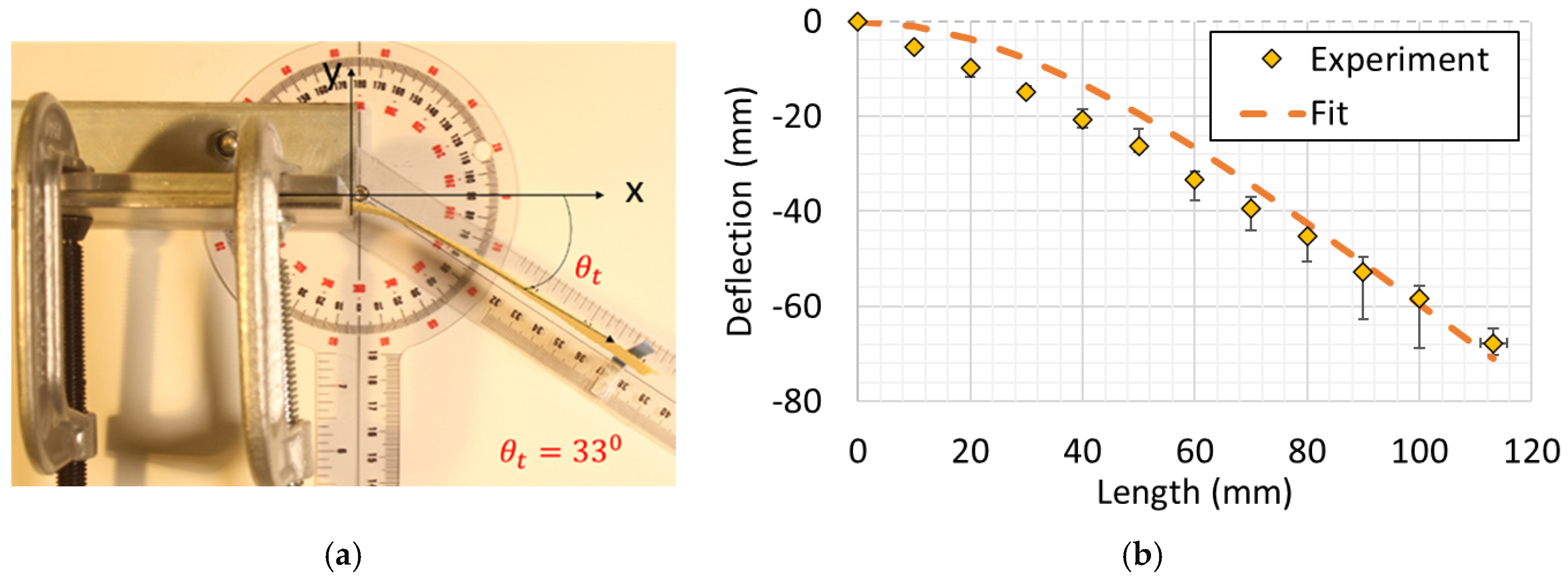
DIA of the photographs obtained in Figure 11a, during the flexibility tests, facilitates the extraction of deflection curves for the fabric samples. Deflections were measured at an approximately 10 mm horizontal spacing for all nine trials conducted across three samples. The measured deflection can be approximated using the theoretical deflection curve for a cantilevered beam under uniform distributed loading, as given by

$$y=-{\displaystyle \frac{w_l}{24E{I}_{cs}}}\left({6L_c}^2{x}^2-4L_c{x}^3+x^4\right)$$

(29)

where $w_l$ is the weight per unit length of the sample, $E{I}_{cs}$ is the flexural rigidity, $L_c$ is the cantilever length, and (x, y) are the measured coordinates on the deflected fabric. The theoretical deflection curve fits obtained using the method of least squares for the measured deflections are plotted in Figure 11b. The flexural rigidity educed from the corresponding fitting curve for neat Kevlar is $48.9{ \mathrm{\mu }\mathrm{Nm}}^2$. The flexural rigidity ($E{I}_{cs}$) is related to the flexural modulus (E) from

$$E{I}_{cs}=E{\displaystyle \frac{b{d}^3}{12}}$$

(30)

where $I_{cs}$ is the moment of inertia in the z-axis of the cross-sectional area of the material, b is the width of the test Kevlar sample (25 mm), and d is the sample thickness (0.61 mm). Using the above expression, the estimated equivalent out-of-plane bending stiffness modulus (E) of the neat Kevlar sample was computed as $102 \mathrm{MPa}$. Next, the equivalent out-of-plane bending stiffness modulus of the nanoparticle-impregnated Kevlar was estimated using the sample testing procedure above.

Figure 11. (a) Neat Kevlar flexibility test; (b) deflection curve fit for measurements.

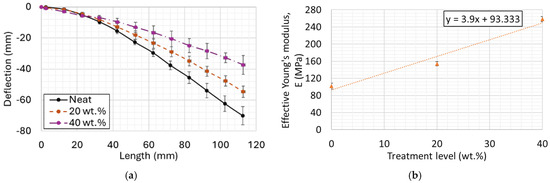
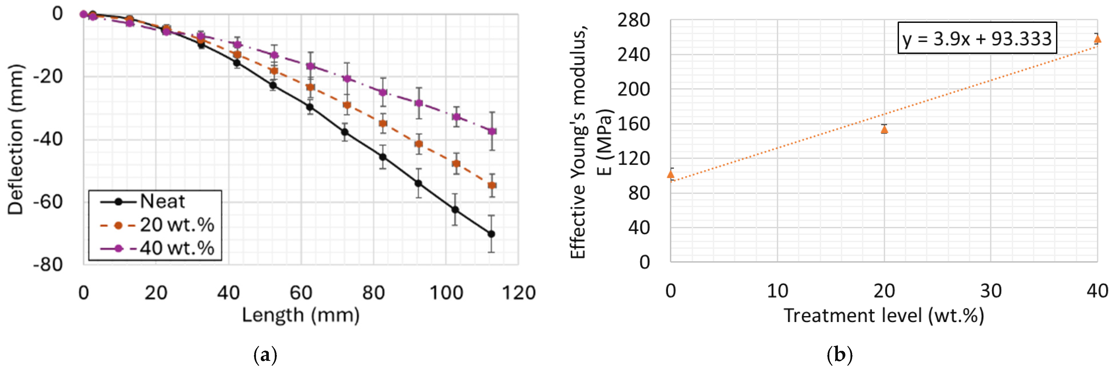
The deflection behavior of Kevlar samples for various nanoparticle treatment levels is illustrated in Figure 12a. The flexural rigidity, extracted from these deflection curves, ranged from 48.9 μN·m² for the neat Kevlar fabric to 121.7 μN·m² for the sample treated with 40 wt.% SNK. Subsequently, as presented in Figure 12b, the calculated flexural modulus which is the Kevlar sample’s equivalent out-of-plane bending stiffness modulus, ranged linearly from 102 MPa for the neat Kevlar to 258 MPa for the 40 wt.% SNK. Although the addition of nanoparticles increases both the weight and the bending stiffness of the fabric, the influence of stiffness appears to be the dominant factor in determining the flexibility characteristics. This observation is consistent with the previously established SEM image analysis [32], which revealed that, at low (<~20 wt.%) treatment levels, the nanoparticles agglomerate in the interstitial spaces between yarn crossover points, whereas at higher levels, they begin to coat the yarn bundle tops. The impregnation of nanoparticles into these interstitial and crossover spaces is believed to restrict the rotational degrees of freedom at yarn crossover points, leading to a significant increase in the overall flexural modulus of the material.

Figure 12. (a) Measured deflection curve profiles; (b) their extracted equivalent out-of-plane bending stiffness modulus for neat, 20 wt.%, and 40 wt.% SNK fabrics.

5.3. Porosity

An undeformed nanoparticle-impregnated Kevlar fabric may have a certain porosity that can be estimated using an optical method. However, porosity is liable to vary as a function of amplitude and the excitation frequency under acoustic loading. In the NIT experiment, white noise was generated, with a low excitation pressure of 80–90 dB, resulting in minimal deformation and negligible resonance-induced changes in porosity. Under such low excitation pressure, the out-of-plane deformation of the fabric was assumed to be minimal. Hence, the displacement induced by any changes in porosity was negligible.

The acquired image was converted to a binary greyscale representation, as shown in Figure 13. The actual Kevlar fabric contained multiple scales of pores. The optical method was only applied with some degree of accuracy to the large interstitial spaces present in the Kevlar fabric. However, there might be numerous minute pores within the yarn bundles and transition zones that could be associated with very high-frequency acoustic phenomena. For simplicity, it was assumed that the porosity arising from yarn bundles and transition zones was negligible, and the porosity was approximated as being due to the pores in the interstitial spaces. This allowed for the estimation of porosity based on the analysis of the greyscale image.

Figure 13. Color and greyscale digital images of neat Kevlar used in analysis.

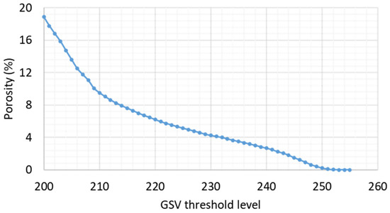
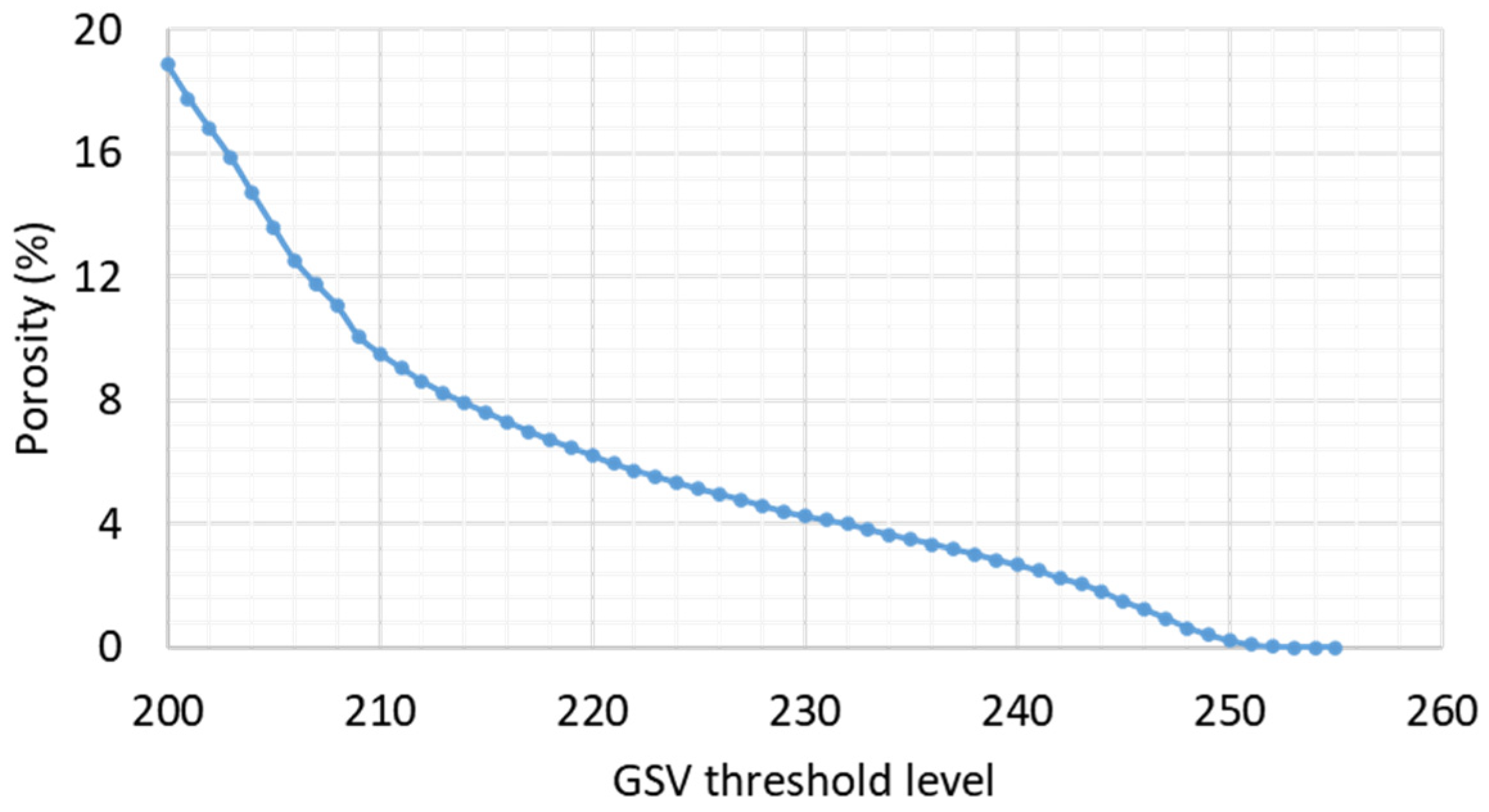
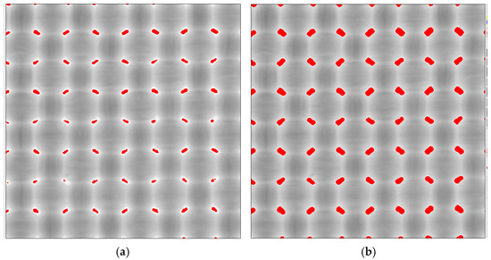
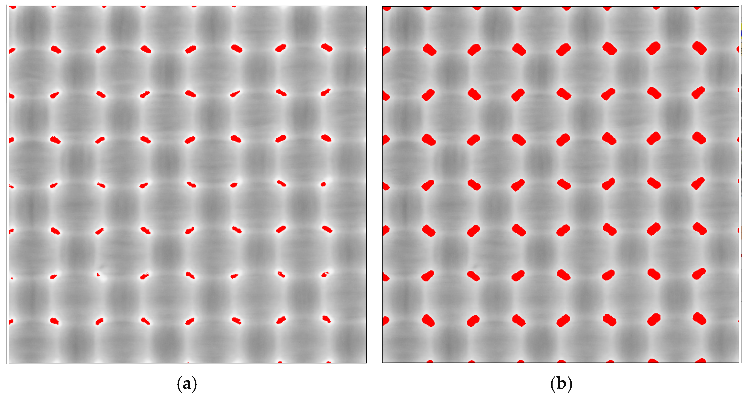
The porosity was then deduced from the ratio of pixel counts corresponding to the sample’s interstitial spaces to the total pixel counts. However, the extent to which the pixels in the interstitial spaces represent the actual pores in those areas was uncertain. Hence, in Figure 14, the porosity is shown for various threshold levels corresponding to the interstitial spots, with greyscale images for 1.5% and 3% porosities shown in Figure 15a and Figure 15b, respectively.

Figure 14. Calculated porosity versus its corresponding greyscale (GSV) threshold levels for neat Kevlar.

Figure 15. Greyscale value threshold maps (995 × 995 pixels) (shown in red) of digital images for neat Kevlar at porosities of 1.5% (a) and 3% (b).

Due to the limitations of the greyscale threshold in identifying interstitial spaces, as shown by the color mapping in Figure 15, it was observed that the porosity might not exceed approximately 3%. Since the exact value of porosity could not be ascertained due to uncertainty in the extent of interstitial spaces in the transition zones between yarn bundles and interstitial spaces, a sensitivity study within this porosity range (1.5–3%) was conducted in Section 5.4.1 to identify the value that best predicts the acoustic behavior of the Kevlar samples in the poroelastic model.

5.4. Sound Transmission Loss

5.4.1. Calibration

Before applying the poroelastic model to the Kevlar samples, the model setup for the circular NIT TL was calibrated using simpler materials, specifically aluminum and neoprene rubber. The aluminum sample provides a stiffness-type TL response, while the neoprene rubber sample provides a limp mass-type TL response. The simulation employs a coupled structural–acoustics model in the frequency domain. The material properties used for the aluminum and neoprene samples in this calibration exercise are presented in Table 5. The exact BCs in the experimental setup are not known precisely because the method used to secure the test sample varies depending on the sample and tube types. In the case of the aluminum plate, the sample was positioned within a hollow tube, and jelly was used to minimize flanking effects around the sample edges. To approximate these complex BCs, a parametric study of different BCs was conducted.

Table 5. Material properties used in FEM simulations for TL.

Material	Property	Value	Unit
Air	Bulk modulus	1.4	MPa
	Density	1.225	kg/m3
Aluminum plate	Young’s modulus	70	GPa
	Density	2700	kg/m3
	Poisson’s ratio	3	%
Neoprene rubber	Young’s modulus	6.14	MPa
	Density	1444	kg/m3
	Poisson’s ratio	0.5	-

Furthermore, a structural damping analysis was performed to further refine the model’s correlation with the experimental data. This damping is an important parameter which is difficult to obtain experimentally; however, it was calibrated numerically.

After completing the BC and the structural damping studies, it was determined that a spring constant of 0.2 MN/m and a structural damping factor of 0.2 provided the best match between the simulated and experimental TL curves for the aluminum plate as presented in Figure 16. The spring constant and structural damping factor were used to tune the compliance and dissipation of the mounting sample and its BC interface. As these phenomenological parameters must be empirically calibrated to a specific experimental setup, it requires baseline testing prior to predicting the transmission loss of new sample iterations. However, this approach does not limit the predictive power of the model as far as the ability to model the inherent qualities of the experimental setup of concern. The differences observed between the simulation model and the experimental data are likely due to residual flanking around the sample edges that may have occurred during the experimental tests.

Figure 16. Comparison of simulated and experimental TL of a 1.2 mm-thick aluminum plate with a spring boundary fixity having a stiffness of 0.2 MN/m and a structural damping factor of 0.2.

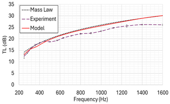
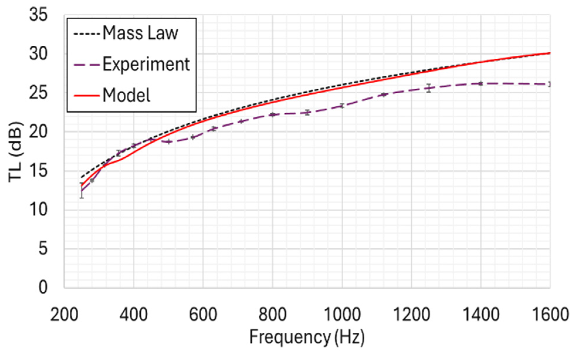
The normal incidence tube (NIT) for TL simulation was further calibrated using the limp mass-type neoprene rubber as shown in Figure 17. A sample mounting frame was attached to a 1.8 mm neoprene rubber sample to hold it securely in place during the experimental tests. Because the precise BCs during the experiment are unknown, a BC study was also performed. A spring BC with a spring constant of 7000 N/m was chosen for the simulation, as it provided the closest agreement with the depth of the TL first dip observed in the experimental data and also matched the mass-law TL. The theoretical mass law assumes an ideal, limp, infinite, and homogeneous barrier. The treated woven fabric is neither limp (it possesses inherent bending stiffness) nor infinite stiff (it exhibits finite boundary resonances). However, the equivalent theoretical mass law is plotted here for comparison to illustrate a limiting behavior for the fabric. As nanoparticle loading is increased, the TL behavior tends more towards the limp mass compared to the neat fabric, especially for higher frequencies. Importantly, the treated fabric does not fully transition from a stiffness-controlled to a purely mass-controlled regime; rather, as it retains other mechanisms such as energy dissipation in the porous media which manifest better at higher frequencies. Hence, the mass-law phenomenon is presented as a limiting case to evaluate the acoustic influence of the added mass in comparison to the other mechanisms at work in the treated fabric.

Figure 17. Comparison of simulated, experimental, and theoretical mass-law TL for neoprene rubber with a spring boundary fixity having a stiffness of 7000 N/m and a structural damping factor of 0.2.

As was the case with the aluminum sheet, the differences observed between the simulation model and the experimental measurements, especially at higher frequencies, are likely due to residual flanking around the sample edges that may have occurred during the experimental testing.

5.4.2. Nanoparticle-Impregnated Kevlar

Following the calibration of the model and the acquisition of the required Kevlar material properties, the model was applied to simulate the TL of neat Kevlar, and the results were compared with experimental measurements. The poroelastic model, described previously, was used for this purpose to replicate the properties of the woven fabric. For computational efficiency and parametric simplification, the Kevlar material was assumed to be isotropic and homogeneous, representing a limp porous material. The input parameters for the model were divided into two categories: primary parameters, which include static airflow resistivity, density, porosity, and Young’s modulus; and inferred parameters, which were derived from the geometric properties of the material and the primary parameters. The porosity of the Kevlar was determined through DIA analysis. Poisson’s ratio in the out-of-plane direction was assumed to be negligible [51]. The characteristic length and tortuosity were estimated, using Equations (15) and (17), respectively. A comprehensive summary of the input parameters used in the simulation model is provided in Table 6. The actual BC in the experiments while close to fixed BC was certainly not fixed; hence, because of the uncertainty in the BC, the BC in the simulation was calibrated in order to account for the loss and compliance at the boundaries. A spring constant of 7000 N/m was found to provide the best match between the simulated and experimental dip locations in the TL curves.

Table 6. Summary of material properties for neat and silica nanoparticle-impregnated Kevlar (SNK) used in the TL simulation model.

		Value			Unit
		Neat	20 wt.%	40 wt.%
Primary parameters	Static flow resistivity ($\mathrm{SFR}$)	15.9	24.6	27.3	MPa.s/m2
	Equivalent out-of-plane bending stiffness modulus ($E$)	102	154	258	MPa
	Porosity (${\epsilon }_p)$	~3	~2	~1	%
	Density (${\rho }_d)$	720	864	1008	kg/m3
Inferred parameters	Poisson’s ratio ($\mathrm{\mu })$	~0.001	~0.001	~0.001	~
	Characteristic length ($L_{ch})$	2.70 × 10−5	2.10 × 10−5	1.96 × 10−5	m
	Tortuosity ($\mathrm{\gamma })$	1.006	1	1	~

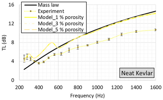
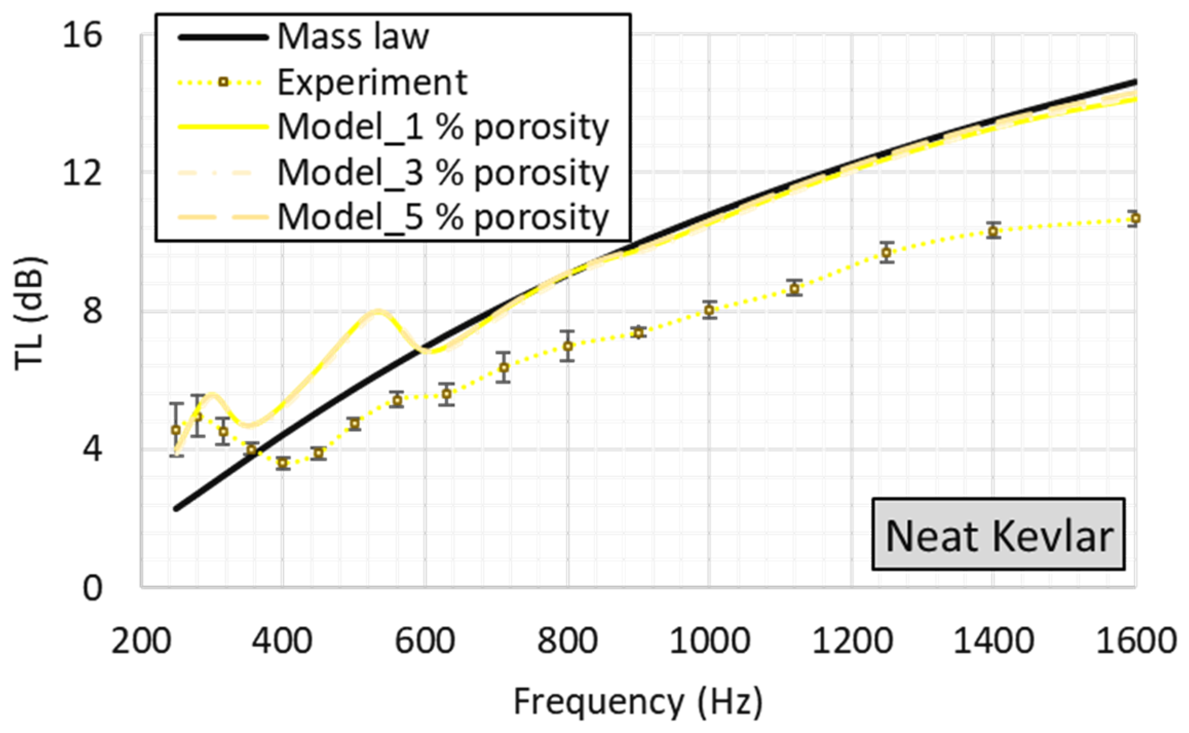
Additionally, a structural damping parameter of 0.2 was obtained from a dedicated damping study and was incorporated in the model to further improve the correlation with the experimental data. The final results obtained from the simulation model are presented in Figure 18.

Figure 18. Comparison of simulated (with different porosities), experimental, and theoretical mass-law TL for neat Kevlar with a spring boundary fixity having a stiffness of 7000 N/m and a structural damping factor of 0.2.

A study was conducted to evaluate the influence of porosity variations (from 1% to 5%) on the simulation model of the neat Kevlar sample, while maintaining all other parameters constant. This study was deemed necessary due to uncertainties in the DIA threshold analysis performed. The results of this study indicated that porosity variations had minimal influence on the simulated TL.

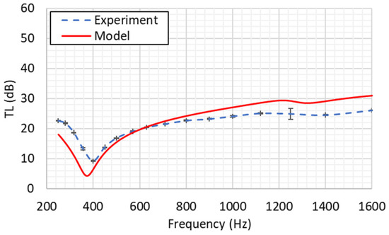
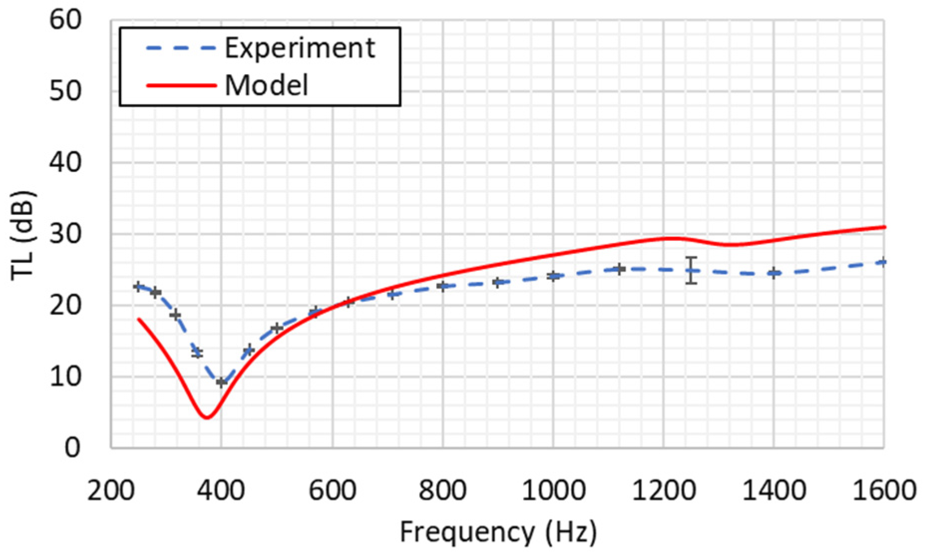
Consequently, porosities ranging from 3% to 1.5%, corresponding to neat Kevlar and the 40 wt.% SNK, respectively, were used the simulation model, reflecting the potential reduction in porosity due to nanoparticle impregnation. The comparison of the simulated TL data for neat Kevlar with the corresponding experimental data revealed a close match in the location of the TL dips, which are attributed to resonance phenomena associated with the sample BCs. Consistent with the trend observed in the calibration data using aluminum and neoprene rubber, the simulation model exhibited an average deviation of ~3.5 dB from the experimental data, particularly in the high-frequency region. This deviation is likely attributable to residual flanking around the sample edges during the experimental setup. Moreover, the current study, which uses Biot’s poroelastic model, assumes uniform pores and flow resistivity. Kevlar, being a material with a hierarchy of pores, responds to flow in different ways. The interstitial pores may have a greater response under certain flow conditions. However, the microscopic pores in the yarn bundle tops may respond differently. Thus, the overall porosity and flow resistivity may differ between no-flow excitation, like in the acoustic case, and flow-based testing, which affects the fabric’s resistivity.

In addition, Biot’s poroelastic model does not account for the hierarchy of pores or the resulting variations in flow resistivity, which are treated as single effective values. In addition, it is noteworthy that the simulation model tends to follow the mass-law TL, which assumes a limp mass barrier.

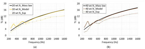
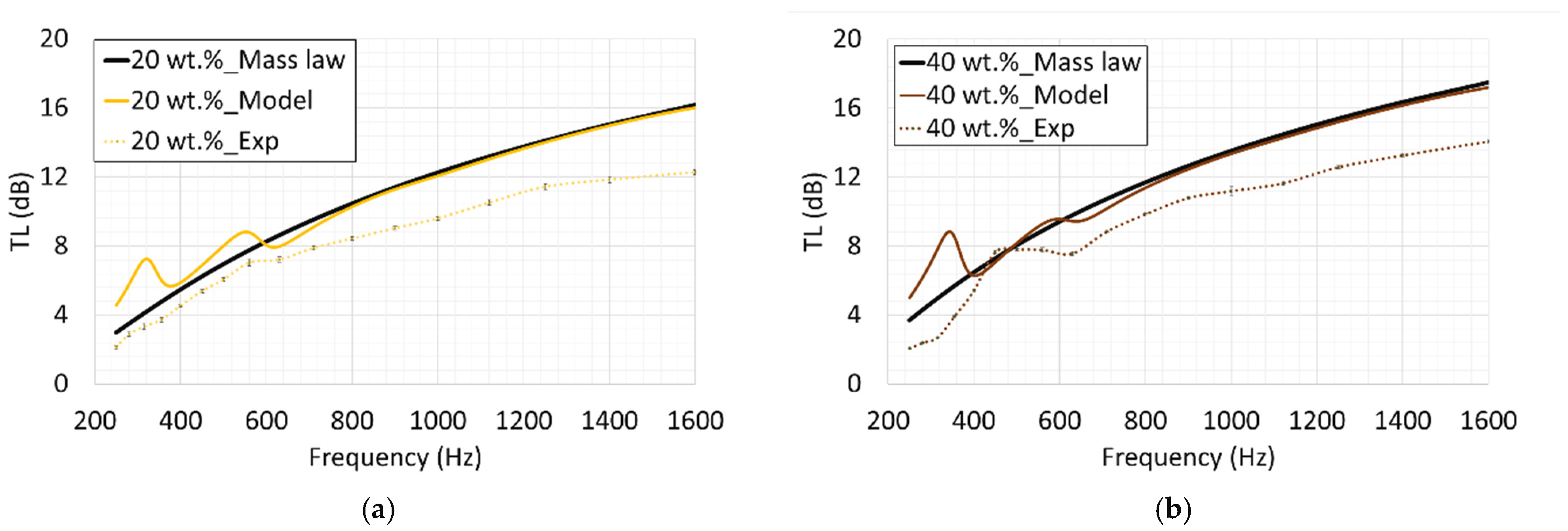
Using the same BCs and simulation procedure that were previously established for predicting the TL of neat Kevlar, and incorporating the material parameters summarized in Table 6, the TLs for SNK with 20 wt.% and 40 wt.% treatments are presented in Figure 19. The simulation results are compared with both theoretical mass-law TL and the experimental data. In the low-frequency region, specifically between 250 and 400 Hz, uncertainties in the experimental BCs lead to discrepancies between the simulation and experimental data. It is important to note, for consistency, that the BCs applied in the model for these two treated Kevlar cases were the same BCs used to calibrate the neat Kevlar simulation, which explains the observed deviations in this frequency range. Furthermore, the average 3.5 dB deviation between the simulation model and the experimental results for both the 20 wt.% and 40 wt.% treated Kevlar samples is consistent with the deviations observed in the calibration data and the neat Kevlar data. It is also observed that the simulation model tends towards the theoretical mass-law TL.

Figure 19. Comparison of simulated, experimental, and theoretical mass-law TL for SNK fabrics with 20 wt.% (a) and 40 wt.% (b) nanoparticle treatments.

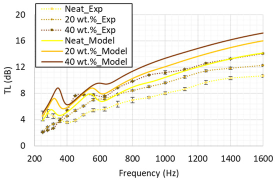
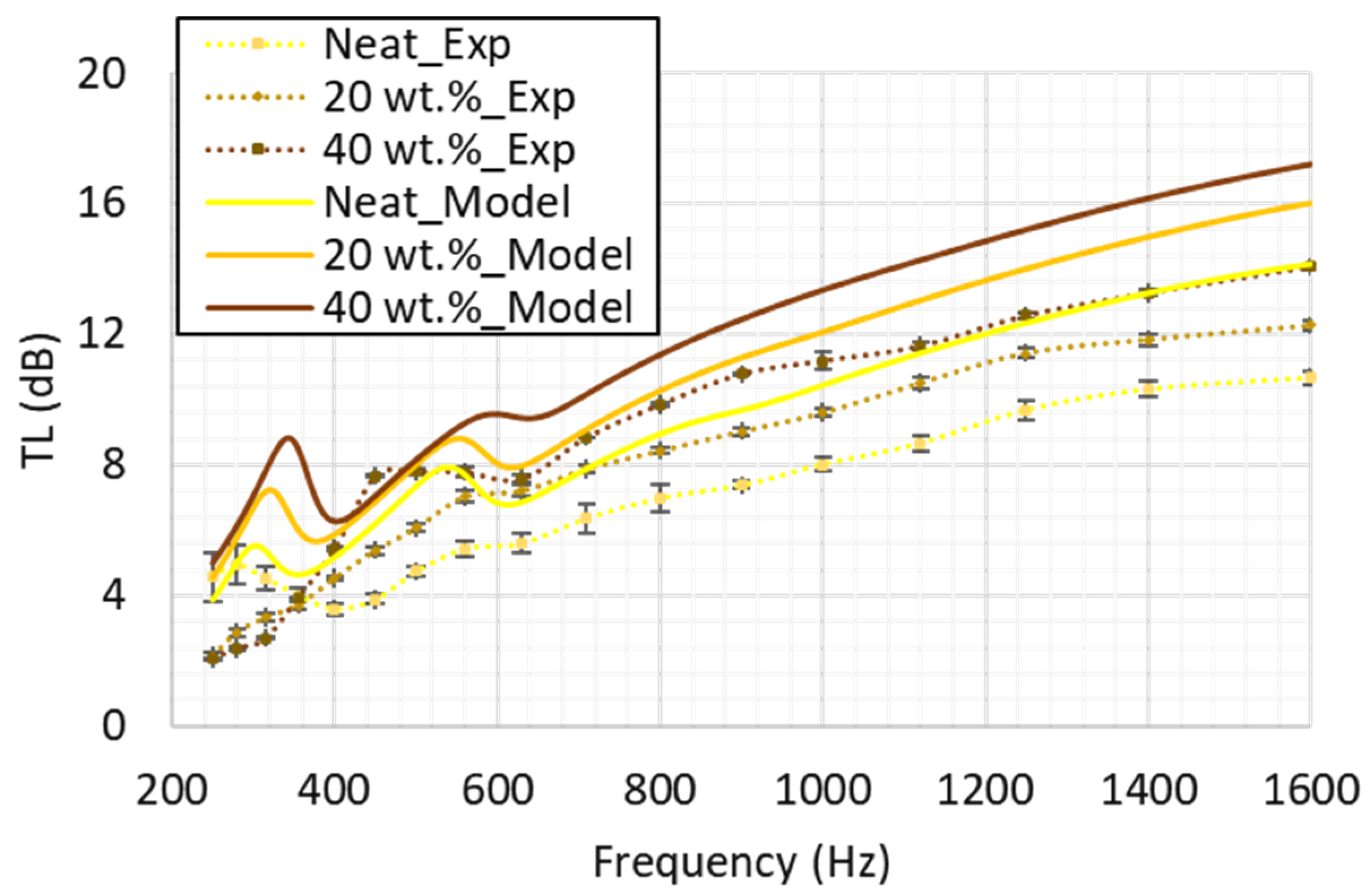
The evolution of both the simulation model and experimental TL from neat Kevlar to 40 wt.% treated Kevlar is presented in Figure 20. Notably, the average increment in the TL predicted by the model, which is approximately 4 dB and appears to be somewhat linear, is consistent with the trend observed in the experimental data. This consistency confirms the accuracy of the nanoparticle treatment process and further validates the simulation model for predicting the TL of SNK fabric.

Figure 20. Comparison of simulated and experimental TL for neat Kevlar, 20 wt.%, and 40 wt.% SNK fabrics.

5.4.3. Verification

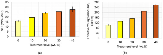
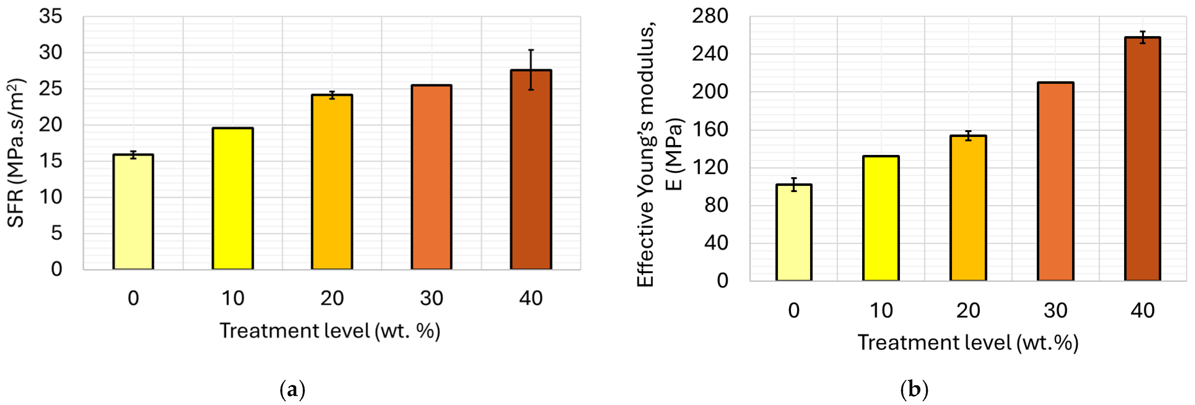
Following the correlation of the simulation model with experimental data, the model’s predictive capabilities were verified by simulating new cases for which the input parameters were not directly measured. Specifically, 10 wt.% and 30 wt.% treated SNK fabric samples were chosen for this validation process. To determine the necessary input parameters for these new cases, a linear regression analysis was performed using the measured values from the neat, 20 wt.%, and 40 wt.% treated SNK fabric samples. For the SFR, a linear regression fit was applied to the data shown in Figure 10, and the resulting regression equation was used to predict the SFR values for the 10 wt.% and 30 wt.% SNK samples. The inferred SFR values obtained from this regression equation were 19.6 MPa.s/m² for the 10 wt.% case and 25.5 MPa.s/m² for the 30 wt.% case. A similar linear regression fit was applied to the data in Figure 12b to infer the equivalent out-of-plane bending stiffness modulus of these new cases, yielding 132 MPa for the 10 wt.% case and 210 MPa for the 30 wt.% case.

Figure 21 presents a comparison of the measured and inferred material parameters used in the simulation model. The plot demonstrates a consistent linear trend for the SFR from neat Kevlar to 40 wt.% SNK, with the inclusion of the inferred values for the 10 wt.% and 30 wt.% cases. As expected, the SFR and equivalent out-of-plane bending stiffness modulus values for the 10 wt.% case fall between those of the neat and 20 wt.% Kevlar samples, and the values for the 30 wt.% case fall between those of the 20 wt.% and 40 wt.% Kevlar samples, which correlates with the expected proportionality between SFR, equivalent out-of-plane bending stiffness modulus, and treatment level. Similar linear regression fits were applied to the porosity and density parameters to infer the values for the new cases. A summary of all inferred parameters for the new cases is provided in Table 7.

Figure 21. Measured and inferred parameters of SNK fabrics used in simulation: (a) SFR; (b) equivalent out-of-plane bending stiffness modulus.

Table 7. Summary of inferred material properties for new SNK cases, as used in the TL simulation model.

Inferred parameters	Value		Unit
	10 wt.%	30 wt.%
Static flow resistivity ($\mathrm{SFR}$)	19.6	25.5	MPa.s/m2
Equivalent out-of-plane bending stiffness modulus ($E$)	132	210	MPa
Porosity (${\epsilon }_p)$	~2.5	~1.5	%
Density (${\rho }_d)$	793	935	kg/m3
Poisson’s ratio ($\mathrm{\mu })$	~0.001	~0.001	~
Characteristic length ($L_{ch})$	2.55 × 10−5	2.89 × 10−5	m
Tortuosity ($\mathrm{\gamma })$	1	1	~

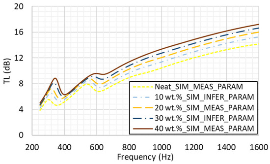
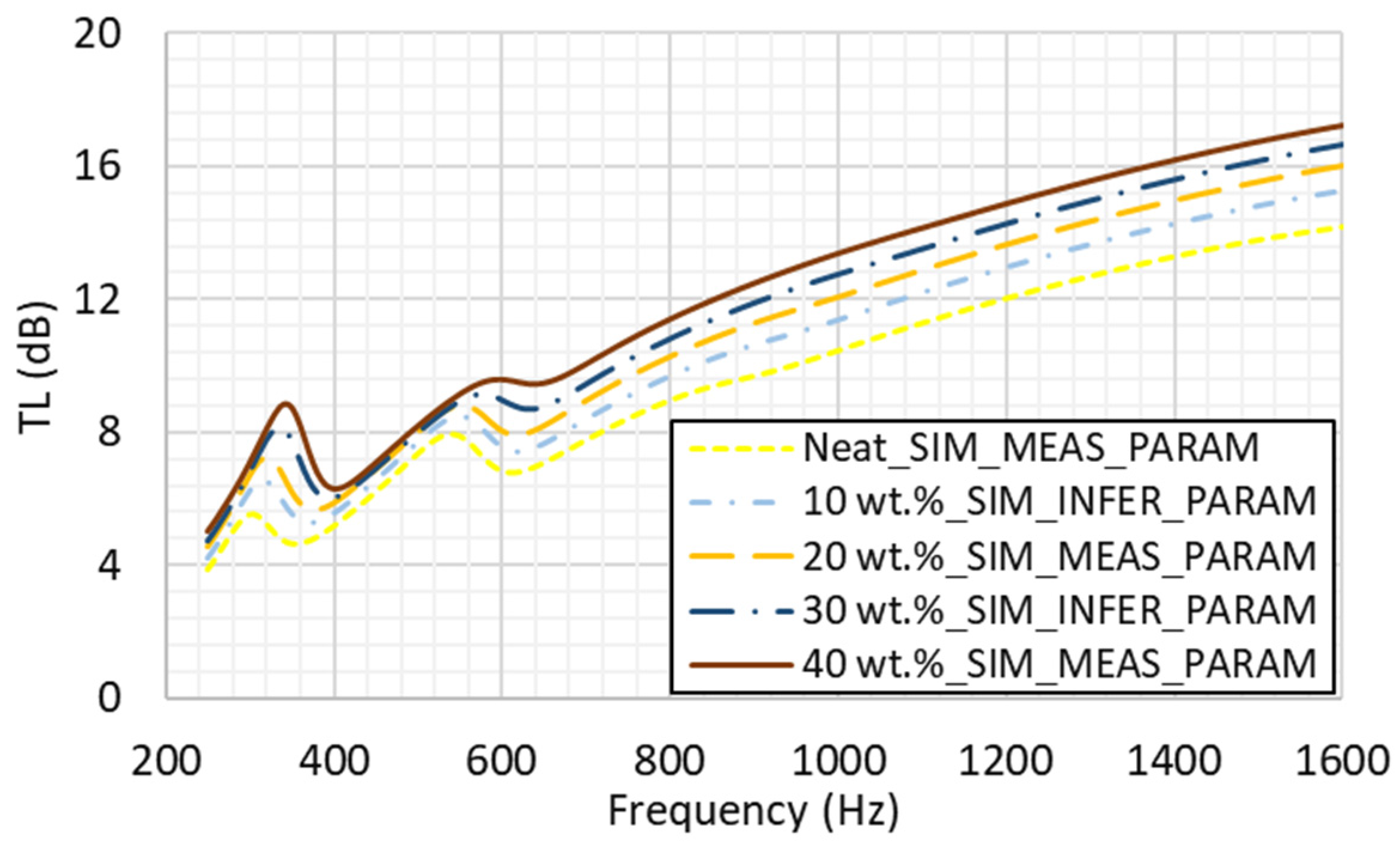
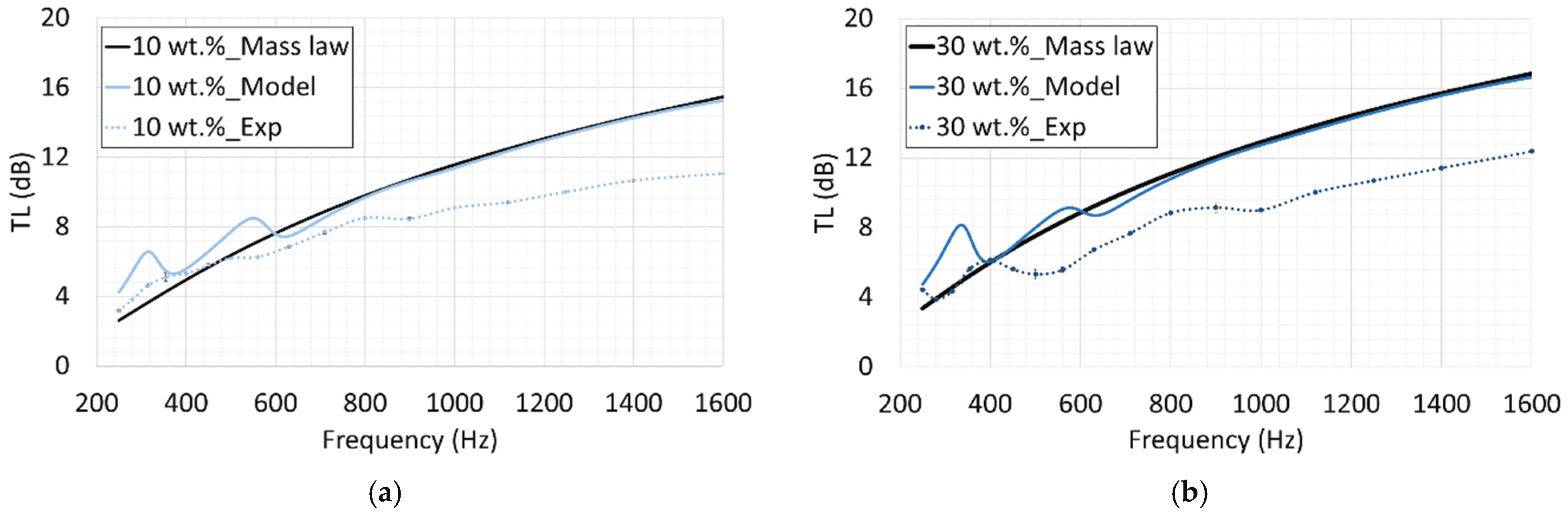
The inferred parameters for the new cases, specifically 10 wt.% and 30 wt.% SNK fabrics, were utilized in the simulation model to predict their corresponding TL values. Figure 22 presents a comparative overview of the model predictions, overlaying the TL curves for cases with both measured and inferred input parameters. The results clearly demonstrate an increasing trend in TL as the nanoparticle wt.% increases. This observation is consistent with the understanding that an increase in treatment level leads to a reduction in pore size and an increase in the mass density of the Kevlar fabric, both of which contribute to an increase in TL. Additionally, the model for the new cases were compared with experiments and mass-law theory predictions (Figure 23). Although the model deviate from the experimental results due to flanking losses and unaccounted uncertain hierarchy of the porosity and flow resistivity parameters used in the simulation model, as observed before, the predicted TL model for both the 10 wt.% and 30 wt.% cases tend towards the mass-law TL. The results obtained from the new cases also confirm the consistency and reliability of the predictive model in simulating the TL of both neat and treated Kevlar samples. The successful prediction of the TL for new SNK fabric cases with different treatment levels serves as a validation of the simulation model, demonstrating its efficacy in predicting the TL of nanoparticle-impregnated Kevlar fabric, thereby offering significant savings in time and cost.

Figure 22. Simulated TL based on measured input parameters for neat Kevlar, 20 wt.%, and 40 wt.% SNK fabrics and inferred input parameters for 10 wt.% and 30 wt.% SNK fabrics.

Figure 23. Comparison of simulated, experimental, and theoretical mass-law TL for SNK fabrics with 10 wt.% (a) and 30 wt.% (b) nanoparticle treatments.

6. Conclusions

This study successfully developed and validated a reduced-order numerical model for the acoustic behavior of silica nanoparticle-impregnated Kevlar (SNK) fabrics, enabling efficient and cost-effective simulations of their sound transmission loss (TL) characteristics. The foundation of this model lies in a coupled poroelastic–acoustic approach, which was rigorously calibrated using experimental data. To facilitate accurate modeling, comprehensive experimental procedures were established to extract critical material properties of SNK, including airflow resistivity, equivalent out-of-plane bending stiffness modulus, and porosity. The model’s predictive capability was further confirmed by applying it to new SNK fabric cases with 10 wt.% and 30 wt.% nanoparticle treatments. For these cases, parameter trends inferred from extensive experimental results for neat, 20 wt.%, and 40 wt.% SNK samples were used to inform the predictions. The accurate TL predictions for these varying treatment levels underscore the model’s efficacy in forecasting the acoustic performance of nanoparticle-impregnated Kevlar, offering substantial time and cost savings in the design and development process.

While Biot’s poroelastic model applied in this study assumes uniform pores within the Kevlar fabric, it is important to acknowledge that Kevlar exhibits a hierarchy of pores, including larger interstitial spaces and smaller pores within yarn bundles. This inherent structural complexity can influence the material’s acoustic behavior in ways not fully captured by a simplified model. Therefore, future research should focus on adapting the poroelastic model to account for this hierarchy of pores to further refine TL performance predictions and explore other acoustic behaviors, such as the sound absorption coefficient. Additionally, the discrepancies observed between acoustic methods, custom tester methods, and the air permeability method in measuring flow resistivity warrant further investigation to ensure consistent and reliable parameter determination for these advanced materials.

The reduced-order model for hybrid structural materials (HSMs) establishes a foundational framework for localized parameter extraction and rapid low-frequency acoustic simulation. By systematically correlating localized physical properties, such as static flow resistivity and effective bending stiffness, with transmission loss, this study advances the fundamental material characterization of nanoparticle-impregnated fabrics. This capability provides an essential computational tool to guide the iterative design of targeted sound-damping composites, particularly in industries like automotive and aerospace. It can streamline the development of sound-damping solutions, addressing emerging noise challenges in quiet propulsion systems. Furthermore, the model holds promise for applications in virtual reality hardware, optimizing acoustic panels in headsets for immersive soundscapes. This capability reduces the need for extensive physical prototyping, enabling faster market entry for innovative acoustic solutions.

References

- Basner, M.; Babisch, W.; Davis, A.; Brink, M.; Clark, C.; Janssen, S.; Stansfeld, S. Auditory and non-auditory effects of noise on health. Lancet 2014, 383, 1325–1332. [Google Scholar] [CrossRef] [Scilit] [PubMed]
- Miedema, H.; Oudshoorn, C.G. Annoyance from transportation noise: Relationships with exposure metrics DNL and DENL and their confidence intervals. Environ. Health Perspect. 2001, 109, 409–416. [Google Scholar] [CrossRef] [Scilit][Green Version]
- Goodman, J.; Grosveld, F. Acoustics and Noise Control in Space Crew Compartments; NASA: Washington, DC, USA, 2015. [Google Scholar]
- Crocker, M.J. Handbook of Acoustics; Wiley-Interscience: New York, NY, USA, 1998; Volume 3. [Google Scholar]
- Kuttruff, H. A simple iteration scheme for the computation of decay constants in enclosures with diffusely reflecting boundaries. J. Acoust. Soc. Am. 1995, 98, 288–293. [Google Scholar] [CrossRef] [Scilit]
- Lee, C.M.; Xu, Y. A modified transfer matrix method for prediction of transmission loss of multilayer acoustic materials. J. Sound Vib. 2009, 326, 290–301. [Google Scholar] [CrossRef] [Scilit]
- Moiser, M. Engineering Acoustics: Introduction to Noise Control, 2nd ed.; Springer: Berlin/Heidelberg, Germany, 2009. [Google Scholar]
- El Kharras, B.; Garoum, M.; Bybi, A. Effect of acoustic enclosure on the sound transmission loss of multi-layered micro-perforated plates. Arch. Acoust. 2024, 49, 241–254. [Google Scholar] [CrossRef] [Scilit]
- Roca, D.; Sal-Anglada, G.; Yago, D.; Cante, J. Coupling multiple resonances for enhancing sound transmission loss of acoustic metamaterials. In Proceedings of the 16th World Congress on Computational Mechanics, Vancouver, BC, Canada, 21–26 July 2024. [Google Scholar]
- Delany, M.E.; Bazley, E.N. Acoustical properties of fibrous absorbent materials. Appl. Acoust. 1970, 3, 105–116. [Google Scholar] [CrossRef] [Scilit]
- Zulkarnain, M.; Harny, I.; Insdrawaty, M.I.; Azman, M.I.F.; Azmi, M.I.A.; Kusrini, E. Study on nature fiber composite for noise material control. Int. J. Technol. 2024, 15, 618–627. [Google Scholar] [CrossRef] [Scilit]
- Jayaraman, P.; Hegde, S.; Reshma, T.; Admaraj, N.H. Influence of fly-ash filler and moisture content on vibrational and acoustic properties of basalt fibre reinforced composites. Adv. Mater. Process. Technol. 2025, 11, 1072–1084. [Google Scholar] [CrossRef] [Scilit]
- AL-Kasar, B.C.M.; Asl, S.K.; Asgharzadeh, H.; Peighambardoust, S.J. Enhancing soundproofing performance of polypropylene nanocomposites for implantable electrodes inside the body through graphene and nanoclay; thermomechanical analysis. AIP Adv. 2024, 14, 125313. [Google Scholar] [CrossRef] [Scilit]
- Sayer, M.; Bektaş, N.B.; Sayman, O. An experimental investigation on the impact behavior of hybrid composite plates. Compos. Struct. 2016, 147, 1256–1262. [Google Scholar] [CrossRef] [Scilit]
- Maev, R.G. Acoustic microscopy for materials characterization. Mater. Charact. Using Nondestruct. Eval. Methods 2019, 104, 161–175. [Google Scholar]
- Miller, J.G. Ultrasonic Nondestructive Characterization of Composites with 3-Dimensional Architectures; NSG-1601; NASA Langley Research Center: Hampton, VA, USA, 1992; pp. 1–29. [Google Scholar]
- Puguan, J.M.C.; Agbayani, D.B.A.; Sadural, A.J.V.; Kim, H. Enhanced low frequency sound absorption of bilayer nanocomposite acoustic absorber laminated with microperforated nanofiber felt. ACS Appl. Polym. Mater. 2023, 5, 8880–8889. [Google Scholar] [CrossRef] [Scilit]
- Dong, Z.; Manimala, J.M.; Sun, C.T. Mechanical behavior of silica nano-particle impregnated Kevlar fabrics. J. Mech. Mater. Struct. 2010, 5, 529–548. [Google Scholar] [CrossRef] [Scilit][Green Version]
- Bablu, M.A.; Manimala, J.M. Mechanisms of ballistic performance enhancement in silica nanoparticle-treated kevlar fabric. J. Compos. Mater. 2022, 56, 2235–2249. [Google Scholar] [CrossRef] [Scilit]
- Smith, N.; Meyyappan, M. Nanostructures and nanoparticles: Sources, processing, and applications in space Exploration. In Nanomaterials: Science and Applications; CRC Press: Boca Raton, FL, USA, 2018. [Google Scholar]
- Marijnissen, J.; Gradon, L. Nanoparticles in Medicine and Environment; Springer: Berlin/Heidelberg, Germany, 2010. [Google Scholar]
- Akinmolayan, O.P.; Manimala, J.M. Acoustic characterization of silica nanoparticle-impregnated Kevlar fabric. Text. Res. J. 2020, 92, 2830–2848. [Google Scholar] [CrossRef] [Scilit]
- Atienzar-Navaroo, R.; Bonet-Aracel, M.; Gisbert-Paya, J.; Dell, A. Sound absorption of textile fabric doped with microcapsule. Appl. Acoust. 2020, 164, 107285. [Google Scholar] [CrossRef] [Scilit]
- Tang, X.; Yan, X. Airflow resistance of acoustical fibrous materials: Measurements, calculations and applications. J. Ind. Text. 2020, 49, 981–1010. [Google Scholar] [CrossRef] [Scilit]
- Akinmolayan, O.P. Acoustic Characterization of Hybrid Structural Materials. Ph.D. Thesis, Oklahoma State University, Stillwater, OK, USA, May 2025. [Google Scholar]
- Biot, M. The theory of propagation of elastic waves in a fluid-saturated porous solid. J. Acoust. Soc. Am. 1952, 24, 168. [Google Scholar]
- Biot, M. Generalized theory of acoustic propagation in porous dissipative media. J. Acoust. Soc. Am. 1962, 34, 1254–1264. [Google Scholar] [CrossRef] [Scilit]
- Allard, J.F.; Atalla, N. Propagation of Sound in Porous Media: Modeling Sound Absorbing Materials, 2nd ed.; Elsevier Applied Science: New York, NY, USA, 2009; pp. 243–307. [Google Scholar]
- Shen, C.; Zeng, F.; Wang, Q.; Hu, Y. Waterborne sound transmission loss in finite double-plate sandwich structures with poroelastic cores. J. Appl. Math. Phys. 2025, 13, 2542–2556. [Google Scholar]
- Biot, M. Theory of propagation of elastic waves in a fluid-saturated porous solid. I. Low-frequency range. J. Acoust. Soc. Am. 1956, 28, 168–178. [Google Scholar] [CrossRef] [Scilit]
- Biot, M. Theory of propagation of elastic waves in a fluid-saturated porous solid. II. Higher frequency range. J. Acoust. Soc. Am. 1956, 28, 179–191. [Google Scholar] [CrossRef] [Scilit]
- Bablu, M. Ballistic Characterization of Meta-Configured Structures. Ph.D. Thesis, Oklahoma State University, Stillwater, OK, USA, 2024. [Google Scholar]
- ASTM E2611-09; Standard Test Method for Measurement of Normal Incidence Sound Transmission of Acoustical Materials Based on the Transfer Matrix Method. ASTM International: West Conshohocken, PA, USA, 2017.
- ISO 9237; Acoustics—Materials for Acoustical Applications—Determination of Airflow Resistance. International Standards Organization: Geneva, Switzerland, 1991.
- Yilmaz, N. Multi-fiber needle-punched nonwoven composites: Effects of heat treatment on sound absorption performance. J. Ind. Text. 2013, 43, 231–246. [Google Scholar] [CrossRef] [Scilit]
- Arumugam, V.; Mishra, R.; Militky, J.; Novak, J. Thermo-acoustic behaviour of 3D knitted spacer fabrics. Fibers Polym. 2015, 16, 2467–2476. [Google Scholar] [CrossRef] [Scilit]
- Tang, X.; Jeong, C.; Yan, X. Prediction of sound absorption based on specific airflow resistance and air permeability of textiles. J. Acoust. Soc. Am. 2018, 144, 100–104. [Google Scholar] [CrossRef] [Scilit] [PubMed]
- Yang, T.; Hu, L.; Petru, M.; Wang, X.; Xiong, X.; Yu, D.; Mishra, R.; Miltky, J. Determination of the permeability coefficient and airflow resistivity of nonwoven materials. Text. Res. J. 2021, 92, 126–146. [Google Scholar] [CrossRef] [Scilit]
- ASTM D1388-14e; Standard Test Method for Stiffness of Fabrics. ASTM International: West Conshohocken, PA, USA, 2014.
- Bear, J. Dynamics of Fluid in Porous Media; Dover Publications: Mineola, NY, USA, 1972. [Google Scholar]
- Allard, J.F.; Champoux, Y. New empirical equations for sound propagation in rigid frame fibrous materials. J. Acoust. Soc. Am. 1992, 91, 3346–3353. [Google Scholar] [CrossRef] [Scilit]
- Gibson, L.J.; Ashby, M.F. Cellular Solids: Structure and Properties, 2nd ed.; Cambridge University Press: Cambridge, UK, 1997. [Google Scholar]
- Pierce, A.; Smith, P. Acoustics: An introduction to its physical principles and applications. Phys. Today 1991, 34, 56–57. [Google Scholar]
- Debergue, P.; Panneton, R.; Atalla, N. Boundary conditions for the weak Formulation of the mixed (u,p) poroelasticity problem. J. Acoust. Soc. Am. 1999, 106, 2383–2390. [Google Scholar] [CrossRef] [Scilit]
- Atalla, N.; Hamdi, M.; Panneton, R. Enhanced weak Integral formulation for the mixed (u_,p_) poroelastic equations. J. Acoust. Soc. Am. 2001, 109, 3065–3086. [Google Scholar] [CrossRef] [Scilit]
- Atalla, N.; Panneton, R.; Debergue, P. A mixed displacement-pressure formulation for poroelastic materials. J. Acoust. Soc. Am. 1998, 104, 1444–1452. [Google Scholar] [CrossRef] [Scilit]
- Atalla, N.; Sgard, F.; Amedin, C. On the modeling of sound radiation from poroelastic materials. J. Acoust. Soc. Am. 2006, 120, 1990. [Google Scholar] [CrossRef] [Scilit]
- Biot, M. Mechanics of deformation and acoustic propagation in porous media. J. Appl. Phys. 1962, 33, 1482–1498. [Google Scholar] [CrossRef] [Scilit]
- Jung, S.; Kim, Y.; Lee, Y. Measurement of sound transmission loss by using impedance tubes. J. Korean Phys. Soc. 2008, 53, 596–600. [Google Scholar] [CrossRef] [Scilit]
- Tao, J.; Wang, P.; Qiu, X.; Pan, J. Static flow resistivity measurements based on the ISO 10534.2 standard impedance tube. Build. Environ. 2015, 94, 853–858. [Google Scholar] [CrossRef] [Scilit]
- Manimala, J.M.; Sun, C.T. Investigation of failure in Kevlar fabric under transverse indentation using a homogenized continuum constitutive model. Text. Res. J. 2013, 84, 388–398. [Google Scholar] [CrossRef] [Scilit]
Disclaimer/Publisher’s Note: The statements, opinions and data contained in all publications are solely those of the individual author(s) and contributor(s) and not of MDPI and/or the editor(s). MDPI and/or the editor(s) disclaim responsibility for any injury to people or property resulting from any ideas, methods, instructions or products referred to in the content. |
© 2026 by the authors. Licensee MDPI, Basel, Switzerland. This article is an open access article distributed under the terms and conditions of the Creative Commons Attribution (CC BY) license.