An Approximate Analytical Method for Predicting Attenuation Due to Ground Effect

Abstract

An approximate analytical model for the variation of A-weighted broadband sound levels with distance over flat acoustically soft ground from a source of known sound power depends on the reduction in low frequency content in noise spectra due to A-weighting. Also, it assumes a weak linear sound speed gradient and a frequency independent attenuation coefficient for air absorption. The model introduces adjustable frequency independent parameters for ground effect, turbulence and atmospheric refraction. An additional parameter allows for the source being located over acoustically hard ground. Predictions of the model are compared with measurements over several ground surfaces. The approximate model predicts a more rapid reduction in sound attenuation due to ground effect with increasing mean propagation path height than the simplified method in a widely used international standard. Moreover, predictions of A-weighted sound levels from onshore wind turbines using the approximate analytical method compare with data and numerical simulations better than the simplified and octave band methods in the international standard and the Swedish standard method.

1. Introduction

There has been a long-standing need to predict noise from fixed industrial premises. More recently predictions are made when assessing the noise impact of onshore wind turbines. These sources may be referred to as broadband since they emit a wide range of frequencies. The frequency content in the received sound is adjusted to correspond to the sensitivity of hearing. Specifically, A-weighting is used which reduces contributions outside the range of speech frequencies between 500 Hz and 4 kHz. The results are expressed as A-weighted sound levels in dB or sound levels in dBA. Despite the increases in computing power and speed that enable relatively accurate and rapid numerical predictions of outdoor sound propagation, there remains a need for less computationally intensive engineering methods. A widely used example is ISO/DIS 9613-2:2024 [1]. Section 7.3.2 of this standard [1] offers a simplified method for calculating attenuation due to ‘soft’ ground effect if only A-weighted sound levels are of interest, the ground is porous or most of it is porous, and the source is not a pure tone. The standard assumes moderate ‘downwind’ conditions. The corresponding expression for attenuation due to soft ground depends only on the mean propagation height and the source to receiver distance. Section 7.3.1 of the standard [1] describes an octave band method and introduces a $G$ factor for distinguishing between ‘hard’ ($G=0$) and ‘soft’ ($G=1$) ground. The octave band method specifies a reduction in ground effect at short range when the distance between source and receiver is less than the height of either the source or the receiver. The standard [1] notes that for source heights of 80 m or more, as might be the case with onshore wind turbines for example, both the general method and the simplified method can overpredict attenuation due to ground effect. To address this, when applying the general (octave band) method, an upper limit of 0.5 is placed on the $G$ factor for ‘soft’ ground and the minimum receiver height to be used is 4 m, even if the actual receiver height is less than 4 m. No corresponding amendments are suggested for the simplified method.

Following Makarewicz et al. [2,3,4] an approximate analytical model can be derived for the propagation of A-weighted levels from a stationary source based on the classical expression for point-to-point propagation over an impedance plane (often called the Weyl-Van der Pol formula). In addition to wave-front spreading and ground effect, the model includes the influences of weak refraction, air absorption and turbulence. The approximation relies on A-weighting to reduce the influence of low frequency content in the source spectra of interest. To allow for refraction, a weak linear sound speed gradient is assumed, and air absorption is included through a frequency independent coefficient.

If the A-weighted source sound power level is denoted by $L_{WA}$ dB, source and receiver heights by $h_s$ and $h_r$ m respectively and their horizontal separation by $d$ m, the A-weighted sound level is given by [4]:

$$L_A=L_{WA}+10\log \left({\displaystyle \frac{E}{4\pi r^2}}\right)-A_{ground}-10\log (1+\alpha d),$$

(1)

where $A_{ground}$ is the attenuation due to ground effect modified by turbulence and refraction given by

$$A_{ground}=10\log \left[1+{\gamma }_g\exp \left(-{\gamma }_{t}d\right){\left({\displaystyle \frac{d}{h_s+h_r}}\right)}^2\right]-10\log \left[1+{\gamma }_R{\left({\displaystyle \frac{d}{h_s+h_r}}\right)}^2\right].$$

(2)

Parameters $E$, ${\gamma }_g$, ${\gamma }_t$, ${\gamma }_R$, and $\alpha$ are adjustable and frequency independent. $E$ is intended to include the effect of the presence and nature of ground near the source on radiation of sound energy from the source ($2\ge E \ge 1$). ${\gamma }_g$, allows for the ‘soft’ ground effect. The lower the surface impedance of the ground, the larger is the value of ${\gamma }_g$. ${\gamma }_t$, allows for the influence of turbulence and is related to the mean square refractive index and the turbulence scale [4]. The larger the value of ${\gamma }_t$ the greater is its influence. ${\gamma }_R$, allows for atmospheric refraction assuming a linear sound speed gradient. Positive values of ${\gamma }_R$ correspond to upward refraction and negative values correspond to downward refraction. The parameter $\alpha$ represents an equivalent frequency independent air absorption coefficient and is assumed to have a value of 14 × 10⁻⁴ nepers per m, corresponding to 10 °C and 70% RH, in subsequent calculations unless stated otherwise.

Section 2 compares predictions of the approximate model with data obtained over continuous soft ground with either a ground mounted jet engine or a loudspeaker as sources of broadband sound. Also, Section 2 compares predictions of the approximate model with data for noise propagating over a single impedance discontinuity from aircraft ground operations and includes a relationship between the ground effect parameter, ${\gamma }_g$, and the ISO9613-2 [1] $G$ factor. Section 3 compares predictions of the approximate model for $A_{ground}$ with those of the simplified method in ISO9613-2 [1] for the variation of attenuation with propagation path height. Section 4 compares predictions and measurements of A-weighted onshore wind turbine sound levels. Concluding remarks are in Section 5. Based on the comparisons with data and numerical predictions, it is suggested that the approximate analytical model provides a more accurate practical engineering method than the simplified method in ISO9613-2 [1] for predicting A-weighted sound levels from fixed broadband sources, including onshore wind turbines, on flat acoustically soft ground.

2. Comparisons with Data

2.1. Continuous Impedance

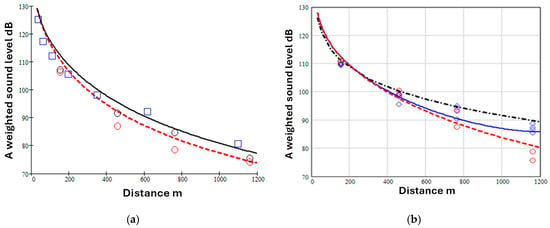
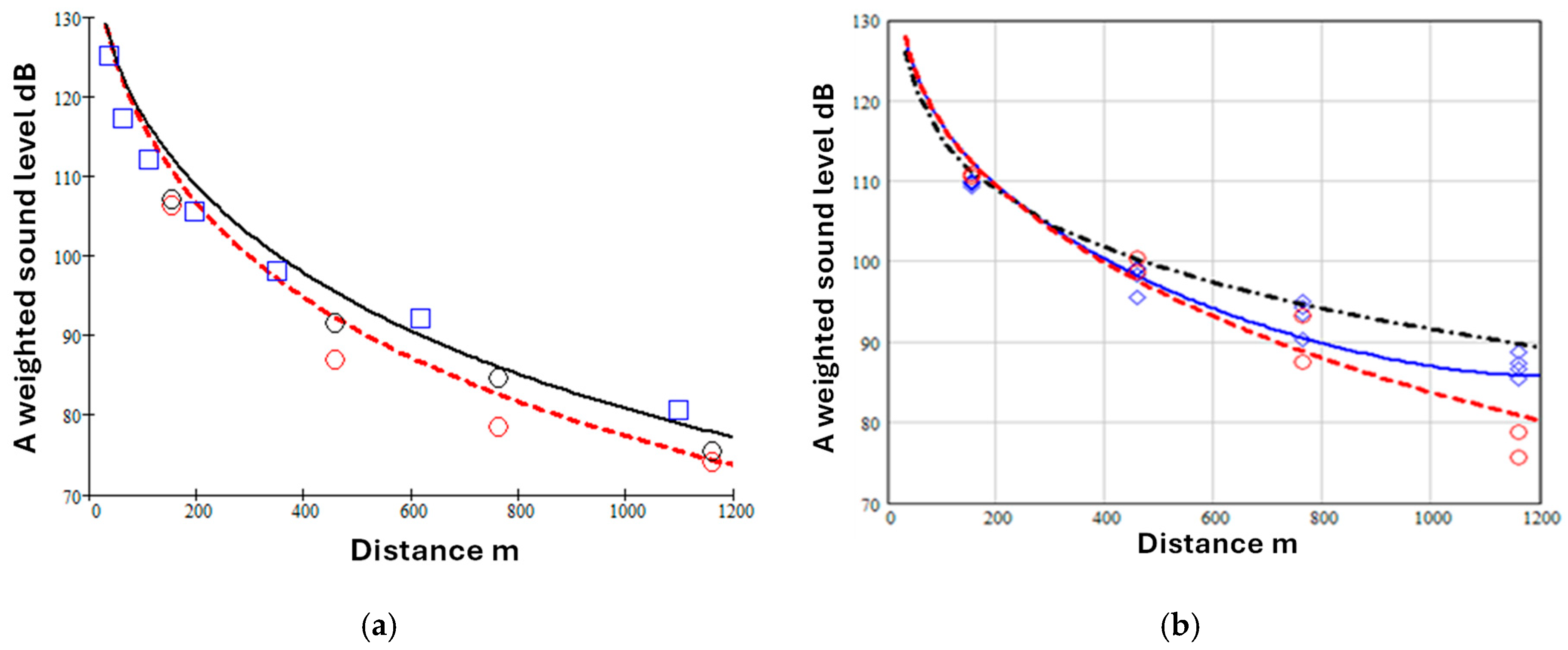
Figure 1a shows A-weighted sound level data at a 1.2 m high receiver for propagation from a fixed jet engine source of broadband sound located on a runway at an airfield [5] in wind speeds less than 6 m s⁻¹ and isothermal conditions (red circles). Also shown in this Figure (open squares) are data for A-weighted levels as a function of range deduced from the corrected level difference measurements by Parkin and Scholes under low wind and isothermal conditions at an airport near Hatfield [6].

Figure 1. (a) A-weighted sound levels due to a fixed jet engine ($L_{WA}=167 \mathrm{d}\mathrm{B}$) during low wind isothermal conditions at Hucknall (source height 2.16 m, receiver height 1.2 m—open circles) [4] and deduced from Parkin and Scholes’ data at Hatfield (source height 1.82 m, receiver height 1.5 m—open squares) [5] compared with predictions of Equations (1) and (2), (solid black line—fitted Hatfield parameters ${\gamma }_g=$ $3\times {10}^{-4}$ and ${\gamma }_t={10}^{-6}$; broken red line—fitted Hucknall parameters ${\gamma }_g=7\times {10}^{-4}$ and ${\gamma }_t={10}^{-7}$) (b) A-weighted levels measured under low wind isothermal conditions (red circles) and downwind conditions (blue diamonds) obtained with receivers 6.4 m above grassland at Hucknall [4], compared with predictions using Equations (1) and (2) (broken red line ${\gamma }_R=$ 0, ${\gamma }_t={10}^{-7}$: solid blue line ${\gamma }_R= -3.5\times {10}^{-5}$, ${\gamma }_t={10}^{-4}$). The black dash-dot line is a prediction using the ISO 9613-2 octave band method [1] with $G=1$.

The continuous black line and broken red line are predictions using Equations (1) and (2), assuming no refraction (${\gamma }_R=0$), $E$ = 2 and values of ${\gamma }_g$ given in the caption. Figure 1b shows data obtained under both low wind isothermal conditions and downward refraction conditions at Hucknall [5] compared with predictions using Equations (1) and (2). For these predictions it has been assumed that E = 1.5 to allow for directivity near the source since it is over an acoustically hard runway.

The low wind isothermal levels measured at Hucknall and Hatfield (Figure 1a) are similar and show a greater attenuation with distance than the levels measured under downwind conditions (Figure 1b). After adjusting values of ${\gamma }_g$, ${\gamma }_t$ and ${\gamma }_R$, Equations (1) and (2) give reasonable agreement with these data. Although the predictions (black dot-dash line) of the ISO9613-2 [1] octave band method in Figure 1b are in reasonable agreement with the data also, they tend to overestimate the measured levels beyond 400 m. Differences between the spectra predicted by the ISO9613-2 [1] octave band method and measurements have been reported elsewhere [4].

Zouboff et al. [7] have carried out a series of measurements in the South of France using a loudspeaker source of broadband noise with maximum energy in the 500 and 1000 Hz octave bands over a flat homogeneous area covered with pebbles and sparse vegetation. Sound levels were measured at a series of microphones located at 80 m, 160 m, 320 m and 640 m from the source. Meteorological parameters including mean air temperature and wind speed at three heights, wind direction, solar radiation and hygrometry were monitored on a 22 m high tower located approximately at the center of the measurement line. 195 ten-minute long samples of sound levels were collected over a range of meteorological conditions and were expressed in terms of the equivalent continuous energy level $L_{\mathrm{A}\mathrm{e}\mathrm{q}}$. Since the ground conditions changed very little, most of the variation may be attributed to meteorological effects.

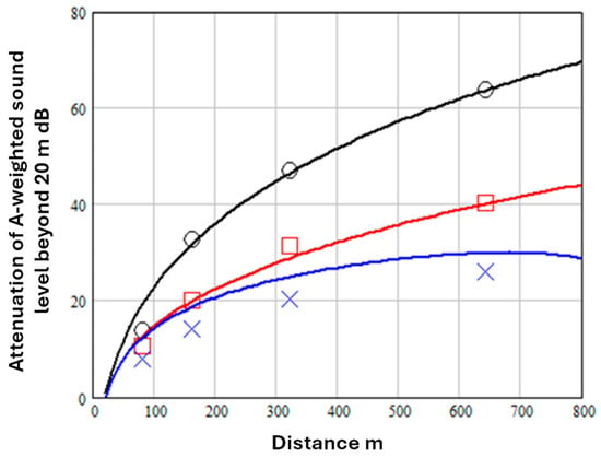
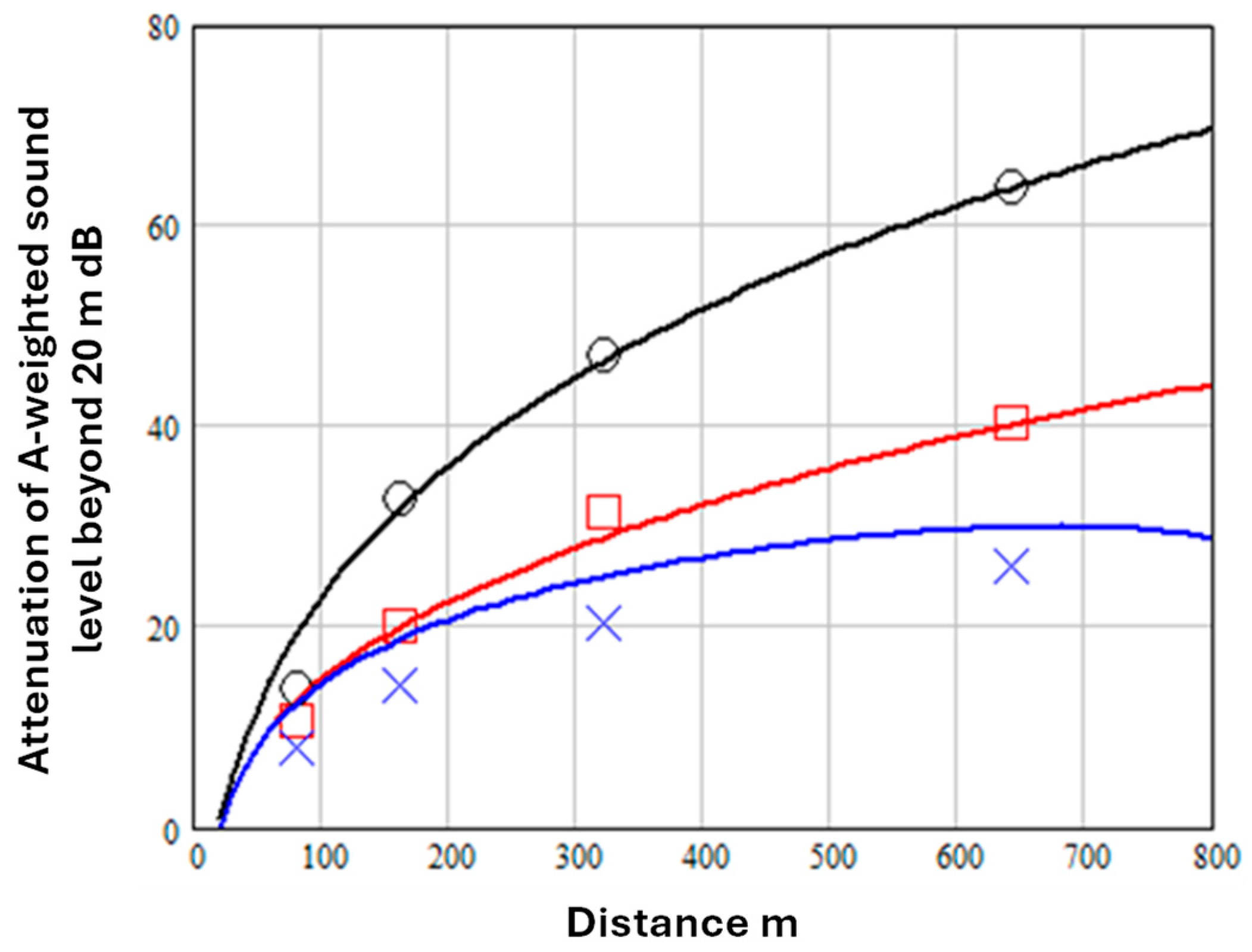
Figure 2 shows the maximum, minimum and mean total attenuation deduced from levels measured at the 1.5 m high microphones after normalizing to a level of 100 dB at 20 m. Predictions of Equations (1) and (2) are shown also after adjusting ${\gamma }_g$ to fit the mean total attenuation (assuming ${\gamma }_R=0$ and ${\gamma }_t={10}^{-6}$) and ${\gamma }_R$ to fit the maximum and minimum attenuation rates. ${\gamma }_t$ is increased for the greater turbulence expected during maximum and minimum attenuation conditions. Source height is assumed to be 1.5 m.

Figure 2. Maximum (black open circles), mean (red open squares) and minimum (blue crosses) measured attenuation beyond 20 m from a 1.5 m high loudspeaker source [7]. Predictions use Equations (1) and (2) with ${\gamma }_g={10}^{-4}$, ${\gamma }_R=$ 0, ${\gamma }_t={10}^{-6}$, red line; ${\gamma }_g={10}^{-4}$, ${\gamma }_R=5\times {10}^{-3}$, ${\gamma }_t={10}^{-5}$ (black line) and ${\gamma }_g={10}^{-6}$, ${\gamma }_R=-1.1\times {10}^{-5}$, ${\gamma }_t={10}^{-4}$ (blue line).

Equations (1) and (2) assume weakly refracting conditions and are not valid if there is strong downwind propagation. Indeed, if the value of ${\gamma }_R$ is made too negative, these equations predict that the A-weighted sound level increases beyond a certain range, as can be seen to be the case with the prediction represented by the solid blue line since it shows decreasing attenuation beyond 700 m. Also, to achieve predictions that correspond approximately to the measured minima, as well as adjusting ${\gamma }_R$, it is found necessary to reduce the value of ${\gamma }_g$, implying acoustically harder ground conditions, This is not unreasonable, since a porous ground surface is likely to be acoustically harder (when wet for example) in conditions where the measured attenuation is minimum.

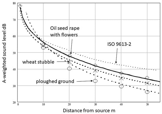
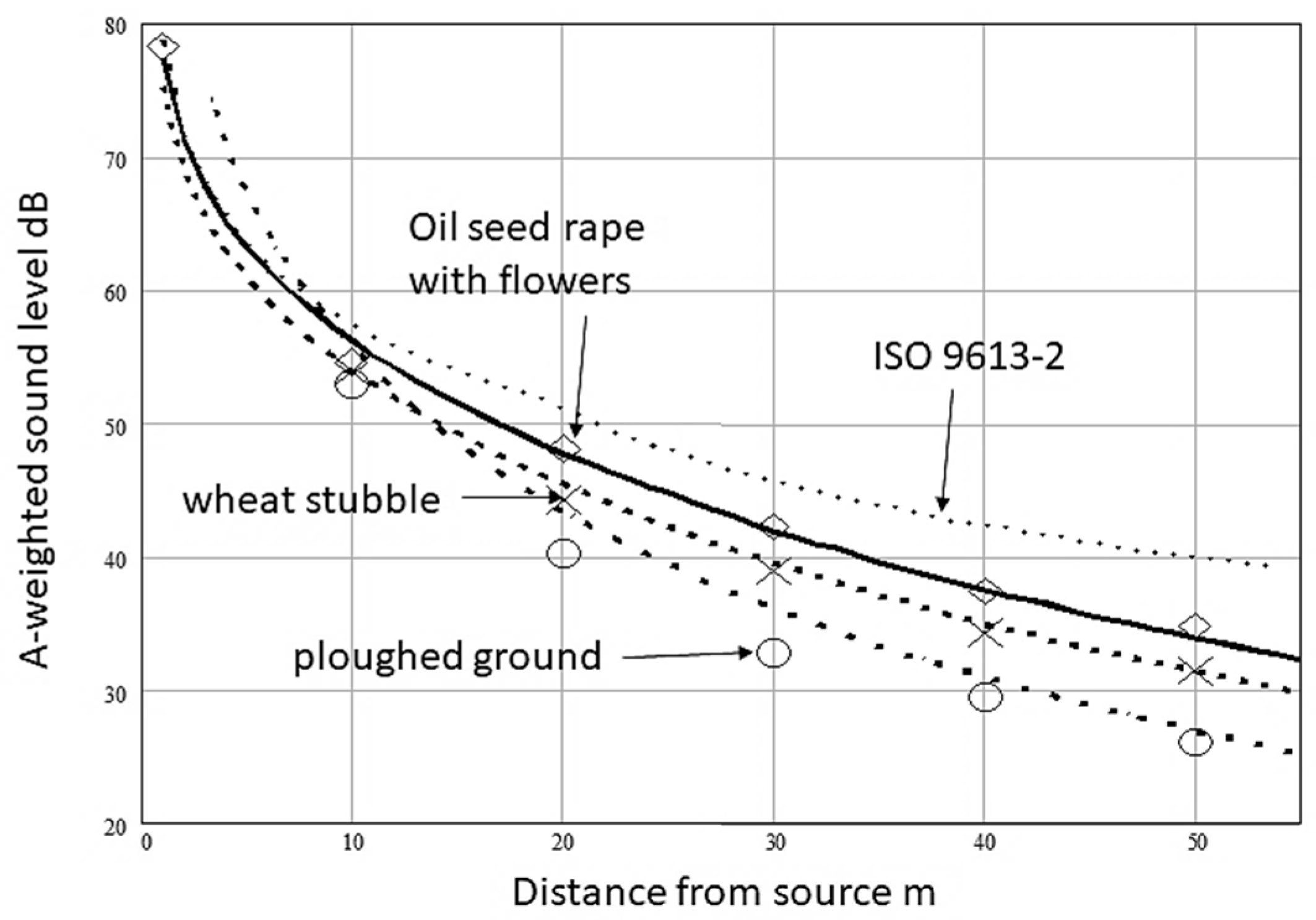
Figure 3 shows average A-weighted sound levels at distances up to 50 m over three cultivated surfaces [8]. Two surfaces were adjacent portions of a field of wheat stubble, one of which had been ploughed. The third surface was covered with oilseed rape plants shortly after flowering. The largest attenuation was measured over the ploughed part of the wheat stubble field. No quantitative meteorological data are available for the measurements over the wheat stubble field. However, in the oilseed rape field, there was a slight wind component (0.9 to 1.9 m/s) between source and receivers. An Electro-Voice loudspeaker was used as a source of broadband sound and assumed to have a height of 1.6 m above the stubble field surface and between 1.6 m and 1.65 m above the soil surface in the oil seed rape field. Since the source output was not calibrated, the data have been normalized to the level measured at 1 m. Also shown (dotted line), are predictions obtained from Equations (1) and (2) with ${\gamma }_R=$ 0, ${\gamma }_t=0$, $\alpha =0$ and fitted values of ${\gamma }_g$ (see Table 1).

Figure 3. A-weighted sound levels relative to that at 1 m measured at 1.2 m height due to a loudspeaker source of broadband sound assumed to have a height of approximately 1.6 m above an oilseed rape field shortly after flowering (open diamonds), and wheat stubble (crosses) and wheat stubble after ploughing (open circles). Also shown are predictions of the ISO9613-2 [1] simplified method (dotted line) and Equations (12) and (2) (broken lines) with ${\gamma }_R=$0, ${\gamma }_t=0$, $\alpha =0$ and fitted values of ${\gamma }_g$ (see Table 1).

Table 1. Fitted values of ${\gamma }_g$ and equivalent values of $G$ acording to Equation (4).

Surface	${\mathit{\gamma }}_{\mathit{g}}$	$\mathit{G}$
Concrete	0.000001	0.090
Pebbles, sparse vegetation	0.00001	0.090
Hatfield grass	0.0003	0.119
French grass	0.0006	0.229
Hucknall grass	0.0007	0.313
Oilseed rape field	0.025	1
Wheat stubble field	0.027	1
Ploughed wheat stubble field	0.031	1

The measured attenuations at 50 m from a loudspeaker source of broad-band noise under slight downwind conditions are between 4 and 10 dB greater than predicted by the ISO9613-2 [1] simplified method for overall A-weighted sound levels (dotted line). The measured differences from the ISO9613-2 [1] predictions are much greater than the expected contribution of air absorption at 50 m.

2.2. Comparisons with Data over Discontinuous Impedance

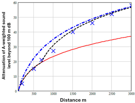
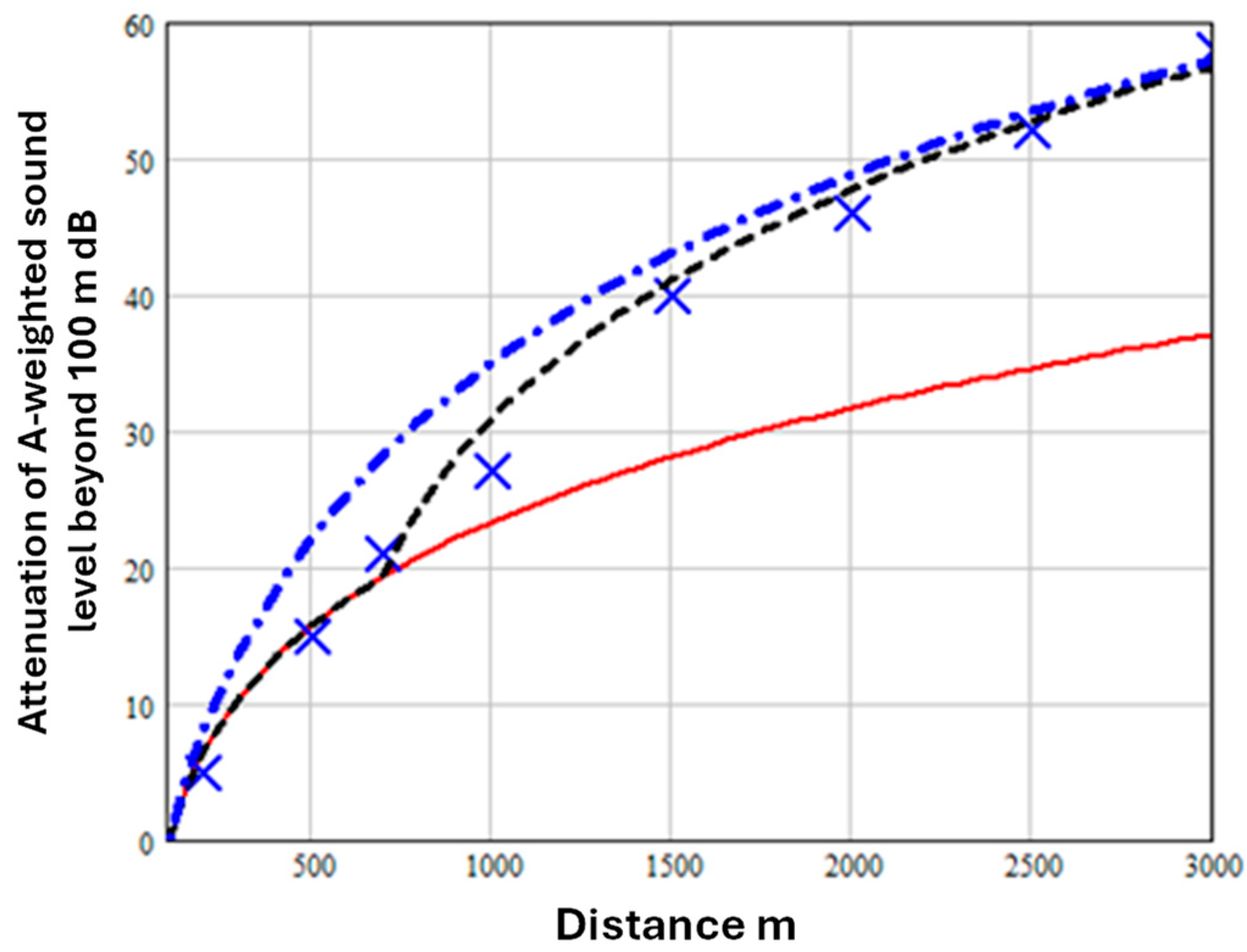
Discontinuities in surface impedance influence the rate of attenuation due to ground effect in low wind isothermal conditions. Measurements of noise levels during aircraft engine run-ups have been made at distances of up to 3 km from the source with the aim of defining ground operation noise contours in the vicinity of airports [9]. Measurements were made for a range of engine power settings during several summer days with near to calm weather conditions (wind speed < 5 m/s, temperature between 20 and 25 °C). Between 7 and 10 measurements were made at every measurement station and averaged. Figure 4 shows examples of the average attenuation measured between a 1.5 m high receiver at a reference distance of 100 m and other 1.5 m high receiver locations between 200 m and 3 km from a stationary jet engine aircraft (notional source height 4.5 m) in the maximum jet noise direction. The change in the measured rate of attenuation between 500 m and 700 m from the source can be attributed to a change in the nature of the ground surface. The aircraft were positioned on a concrete apron, and the surrounding area was either soil or grass. A change in ground impedance at $∆$ m from the source is included through Equation (3).

$$\begin{array}{cc}{\gamma }_g\hfill & ={\gamma }_1,\hspace{1em}\hspace{1em}\hspace{1em}d\le ∆,\hfill \\ & ={\gamma }_2\left({\displaystyle \frac{d-∆}{d}}\right),\hspace{1em}d>∆\hfill \end{array}$$

(3)

Figure 4. Data for the attenuation of A-weighted levels measured under low wind isothermal conditions (blue crosses) [9] compared with predictions of Equation (1) with ${\gamma }_R=$ 0, ${\gamma }_t={10}^{-6}$ and ground parameter ${\gamma }_g=$ ${\gamma }_2=$ $6\times {10}^{-4}$ (dash-dot blue line) or ${{\gamma }_g=\gamma }_1={10}^{-6}$ (continuous red line). The broken black line is the prediction using Equations (1)–(3) with $∆=700$ m.

In Figure 4, the dash-dot blue line is the prediction assuming ${\gamma }_g={\gamma }_2=6\times {10}^{-4}$ for the whole range and the continuous red line is the prediction with ${\gamma }_g={\gamma }_1={10}^{-6}$ for the whole range. The broken black line is the prediction using Equations (1)–(3) with $∆=700$ m and is a reasonable fit to the data.

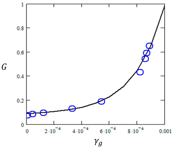
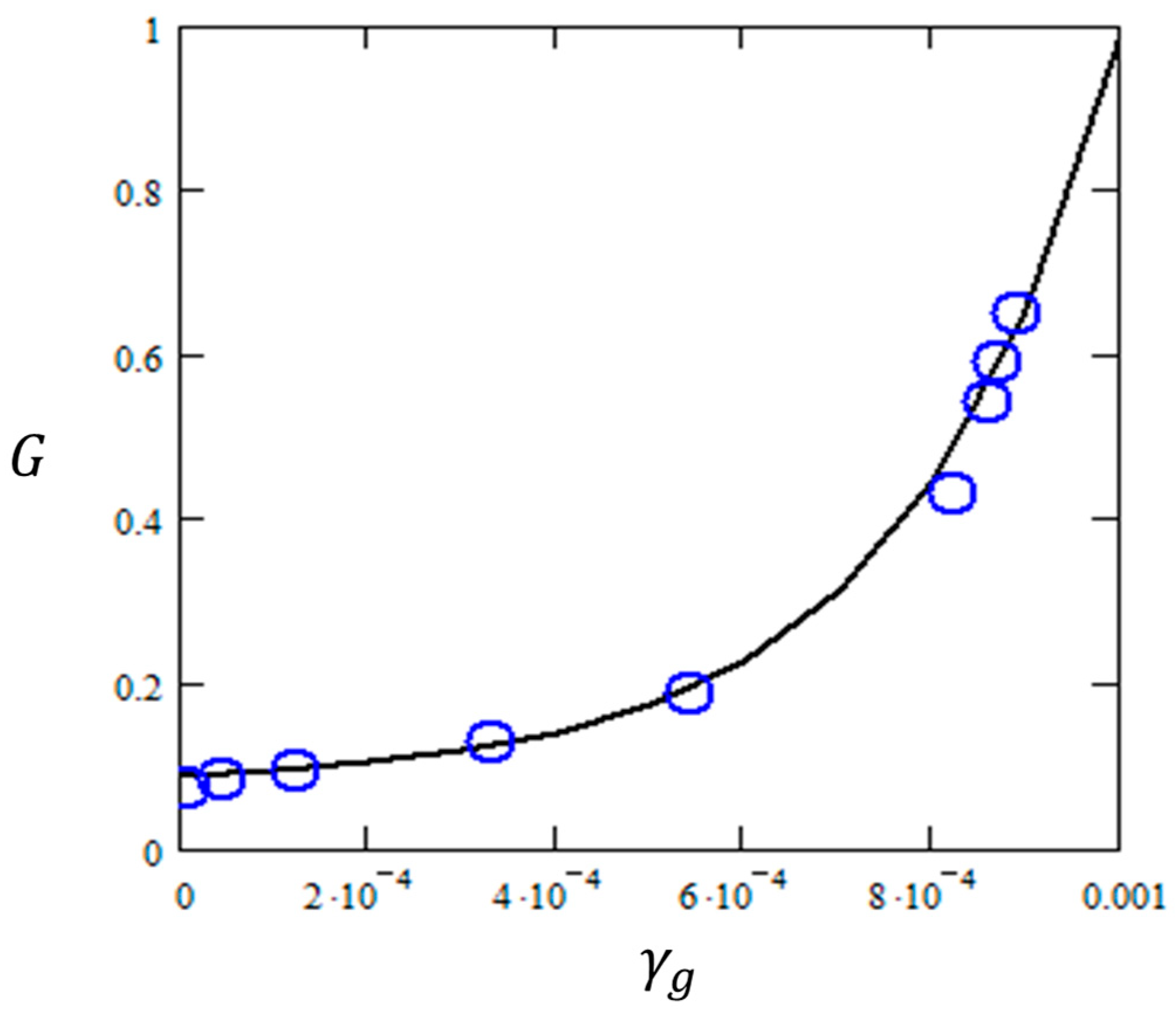
From a series of outdoor measurements and calculations, Golebiewski [10] has suggested equivalences between values of ${\gamma }_g$ and values of the $G$ factor used in the ISO9613-2 octave band method [1] shown by the open blue circles in Figure 5.

Figure 5. Relationships between values of ${\gamma }_g$ and $G$ from Table 2 in ref. [10] (open blue circles). The continuous (black) line is a prediction using Equation (4).

The continuous line is the curve given by Equation (4).

$$G=0.01\left(e^{4500{\gamma }_g}+8\right),G\le 1.$$

(4)

Table 1 lists the values of ${\gamma }_g$ from fitting the data in Figure 1, Figure 2, Figure 3 and Figure 4 using Equations (1)–(4) and corresponding values of $G$.

3. Predicted Variation with Propagation Path Height

According to ISO9613-2:2024 [1], if much of the ground is porous and the sound is not a pure tone, the ground attenuation (dB) can be calculated from

$$A_{ground}=4.8-\left({\displaystyle \frac{2h_m}{d}}\right)\left(17+{\displaystyle \frac{300}{d}}\right)\ge 0 \mathrm{d}\mathrm{B}.$$

(5)

where $h_m$ is the mean height of the propagation path above the ground and negative values of $A_{ground}$ arising from the formula in (5) are set to zero.

When calculating the overall A-weighted sound level and using Equation (5) for attenuation due to ground effect it is necessary to include the directivity correction given by Equation (6) [1].

$$D=10 {\log }_{10}\left\{1+\left(d_p^2+(h_s-h_r{)}^2\right)/\left(d_p^2+(h_s+h_r{)}^2\right)\right\}.$$

(6)

This accounts for the increase in sound power level of the source due to reflections from the ground (assumed to be ‘hard’) near the source. It is equivalent to the term involving the parameter E in Equation (1).

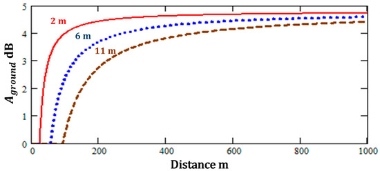
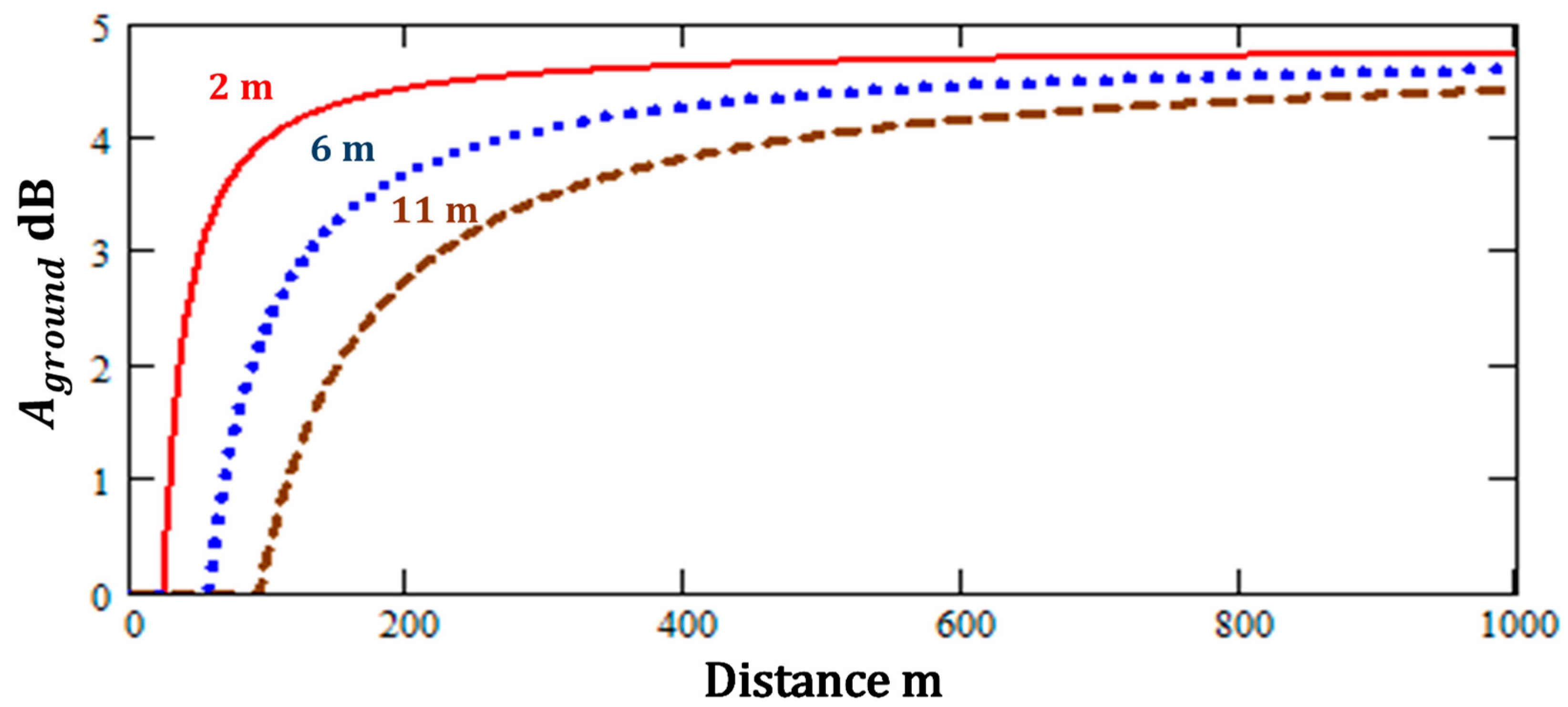
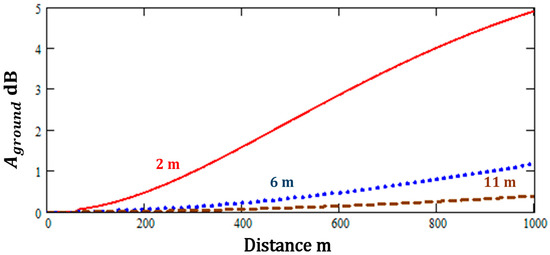
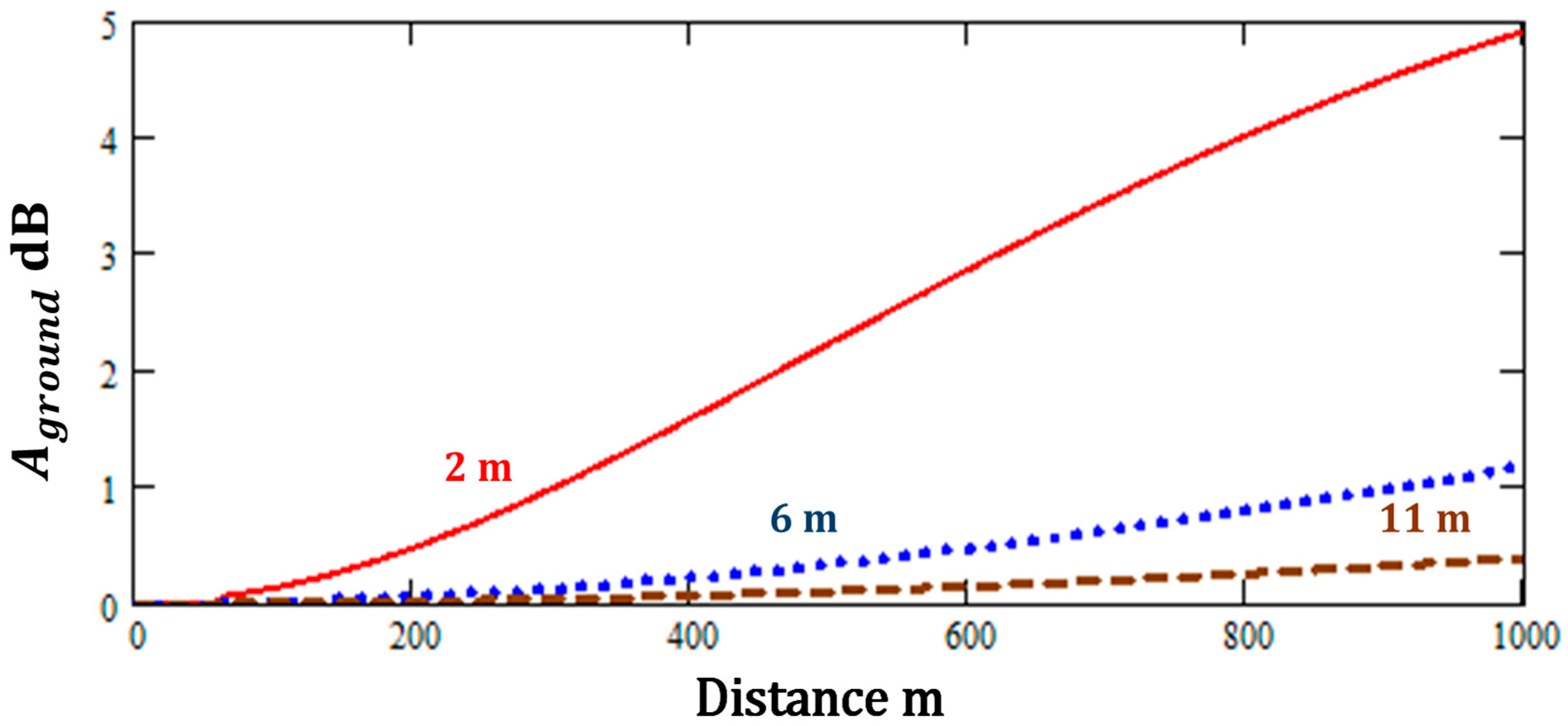
Figure 6 shows predictions of Equation (5) for source heights of 2, 10 and 20 m with a fixed receiver height of 2 m.

Figure 6. Predictions of Equation (5) for mean propagation heights of 2 m, 6 m, and 11 m.

According to the ISO9613-2 [1] simplified method [1], increasing the mean propagation height ($h_m$) increases the distance from the source over which the attenuation due to ground effect is 0 dB. A corresponding provision in the UK Calculation of Road Traffic Noise scheme [11] is that the attenuation due to ground effect is zero if $h_m>\left(d+5\right)/6$. However, the simplified scheme predicts that the attenuation due to soft ground effect approaches 4 dB at 500 m even for mean propagation heights of 11 m.

Figure 7 shows corresponding predictions of Equations (2) and (3) with ${\gamma }_1=2\times {10}^{-6}$, ${\gamma }_2=5\times {10}^{-5}$, $∆=60 \mathrm{m}$ (i.e., the source is over a harder area of ground which extends to 60 m from the source), ${\gamma }_t={10}^{-6}$, and ${\gamma }_R=-2\times {10}^{-6}$. These values have been chosen so that the approximate analytical method predicts a value of $A_{ground}$ of nearly 5 dB at 1 km which is comparable with that predicted by the ISO9613-2 [1] simplified method with $h_m$ = 2 m. However, Equations (2) and (3) predict that the attenuation due ‘soft’ ground effect decreases significantly with increasing source height above 2 m. Indeed, if the mean propagation height is 11 m, the attenuation due to ground effect predicted by the approximate analytical method is less than 1 dB for ranges up to 1 km.

Figure 7. Predictions of Equations (2) and (3) with ${\gamma }_1=2\times {10}^{-6}$, ${\gamma }_2=5\times {10}^{-5}$, $∆ =60 \mathrm{m}$, ${\gamma }_t= {10}^{-6}$, and ${\gamma }_R= -2\times {10}^{-6}$ for mean propagation heights of 2 m, 6 m, and 11 m.

4. Measurements and Predictions of A-Weighted Sound Levels from Onshore Wind Turbines

Many predictions of wind turbine noise are made using the ISO9613-2:2024 octave band method [1]. The relevant equations are not reproduced here for the sake of brevity. The standard recommends that the wind turbine source be regarded as a point source at hub height and that, for predictions over ‘soft’ ground, $G\le 0.5$ and that, if the actual receiver height is less than 4 m, the receiver height should be set at 4 m.

The ISO simplified method can be augmented to include air absorption through Equation (7) which predicts the A-weighted sound pressure level as a function of distance.

$$L_{pA}=L_{WA}-10\log \left(2\pi r^2\right)-A_{ground}+D-10\log (1+\alpha d).$$

(7)

where $D$ is given by Equation (5) and $\alpha$ is the adjustable frequency-independent parameter used in Equation (1).

Forssen et al. [12] have made measurements with 1.7 m high receivers of the sound levels 530 m from a three bladed wind turbine (Enercon E66) with rotor diameter 70 m and hub height 65 m over flat agricultural land (no trees or bushes), under downwind conditions. The variation of A-weighted sound power level was determined for wind speeds between 5 and 12 m s⁻¹ measured at a height of 10 m. The measured levels were compared with predictions obtained with a numerical Parabolic Equation (PE) model, the NORD2000 scheme [13] and the Swedish standard method [14] given by Equation (8).

$$L_{pA}=L_{WA}-8-20\log r-0.005r.$$

(8)

where $r$ m is the distance from the source and the factor 0.005 is intended to account for air attenuation and the losses due to the ground reflection.

According to Forssen et al. [12], Equation (8) predicts an immission level at 530 m within one standard deviation ($\pm 4.7$ dB) of the mean measured values and that, at this range (530 m), the predictions are not improved by taking meteorological conditions into account with either the NORD2000 scheme or the PE model.

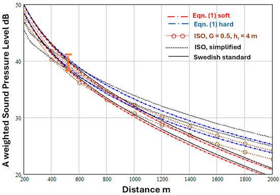
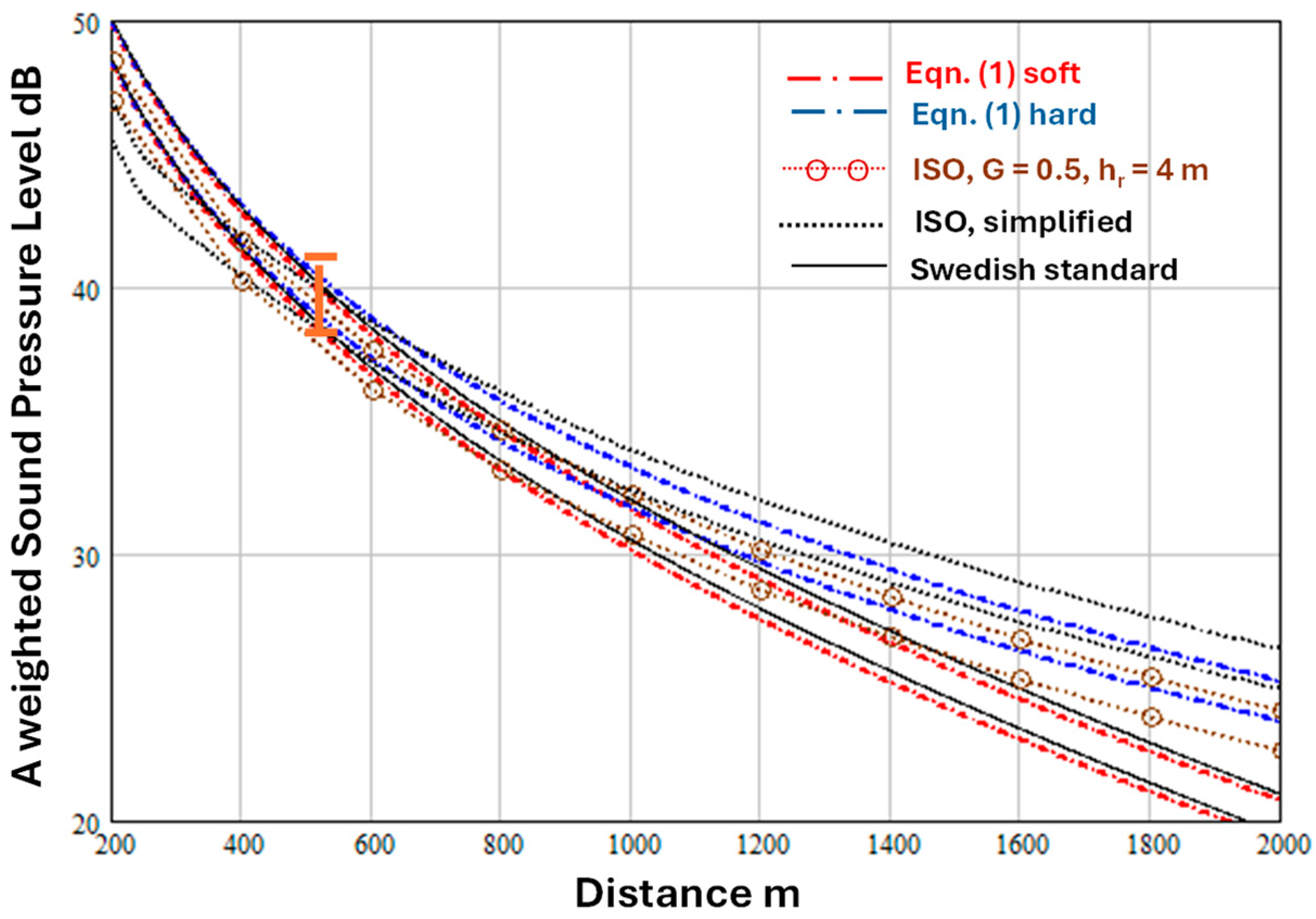
Figure 8 shows predictions of Equations (1) and (2) for a source height ($h_s$) of 65 m, receiver height ($h_r$) of 1.7 m and distances from 200 m to 2 km, with ${\gamma }_t={10}^{-6}$, ${\gamma }_R=-4\times {10}^{-6}$. Also shown in Figure 8 are predictions of Equations (7) and (8) and the ISO9613-2 [1] octave band method with $G=0.5$ and $h_r=4$ m.

Figure 8. Predicted variation of A-weighted sound level with distance according to Equations (1) and (2) for a source height of 65 m, receiver height of 1.7 m, the values of $L_{WA}=105 \mathrm{a}\mathrm{n}\mathrm{d} 103.5$ dB correspond to the highest and lowest sound power levels deduced for wind speeds between 10 and 12 m s⁻¹, ${\gamma }_t= {10}^{-6}$, ${\gamma }_R= -1\times {10}^{-6}$ (weak downward refraction), ${\gamma }_g=0.002$ and ${10}^{-6}$ represent acoustically soft and hard ground respectively (dash dot red and blue lines). Also shown are predictions of Equation (8) (continuous black lines), Equation (7) (dotted black lines) and the ISO9613-2 [1] octave band method with $G=0.5$ and $h_r=4$ m (joined open brown circles). The (orange) error bars at 530 m represent the range of immission levels measured by the 1.5 m high receiver [12].

The sound power levels, $L_{WA}$, deduced from measurements during wind speeds between 10 and 12 m s⁻¹ varied between $105$ and 103.5 dB [12] so both values are used in the predictions. Values of ${\gamma }_g$ (0.00001 and 0.002) are assumed to represent ‘hard’ and ‘soft’ ground respectively.

To make predictions with the ISO9613-2 [1] octave band method the A-weighted sound power levels and air absorption values listed in Table 2 have been used. The octave band sound power levels are an average of the A-weighted spectra for many types of wind turbines Figure 10A in [15]. The total A-weighted sound power level $L_{WA}$ corresponding to the octave band levels in Table 2 is 106.4 dB. However, the levels assumed for subsequent predictions with the ISO9613-2 [1] octave band method have been adjusted to match the A-weighted source power levels used for the predictions with Equations (1), (2), (7) and (8) and the ISO9613-2 [1] simplified method. All predictions are within the range of measured A-weighted sound levels at 530 m. However, the variation with distance predicted by the ISO octave band method differs from that predicted by the other methods. Both ISO methods predict less attenuation than Equations (1) and (2) beyond 1200 m but more attenuation below 400 m. The predictions of Equations (1) and (2) for ‘soft’ ground (${\gamma }_g=0.002$) and Equation (8) (the Swedish standard method) are very close.

Table 2. Average octave band A-weighted wind turbine sound power levels and air absorption.

Octave Band Center Frequency Hz	A-Weighted Sound Power Level dB	Air Absorption dB/km
63	87.1	0.12
125	94.2	0.41
250	98.5	1.04
500	100.6	1.93
1000	101.1	3.66
2000	98.6	9.66
4000	92.6	32.8

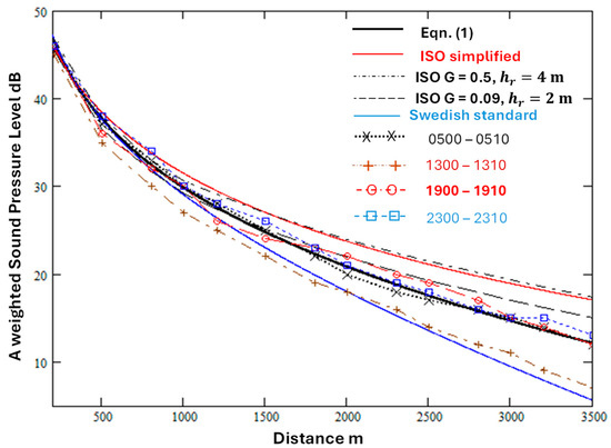
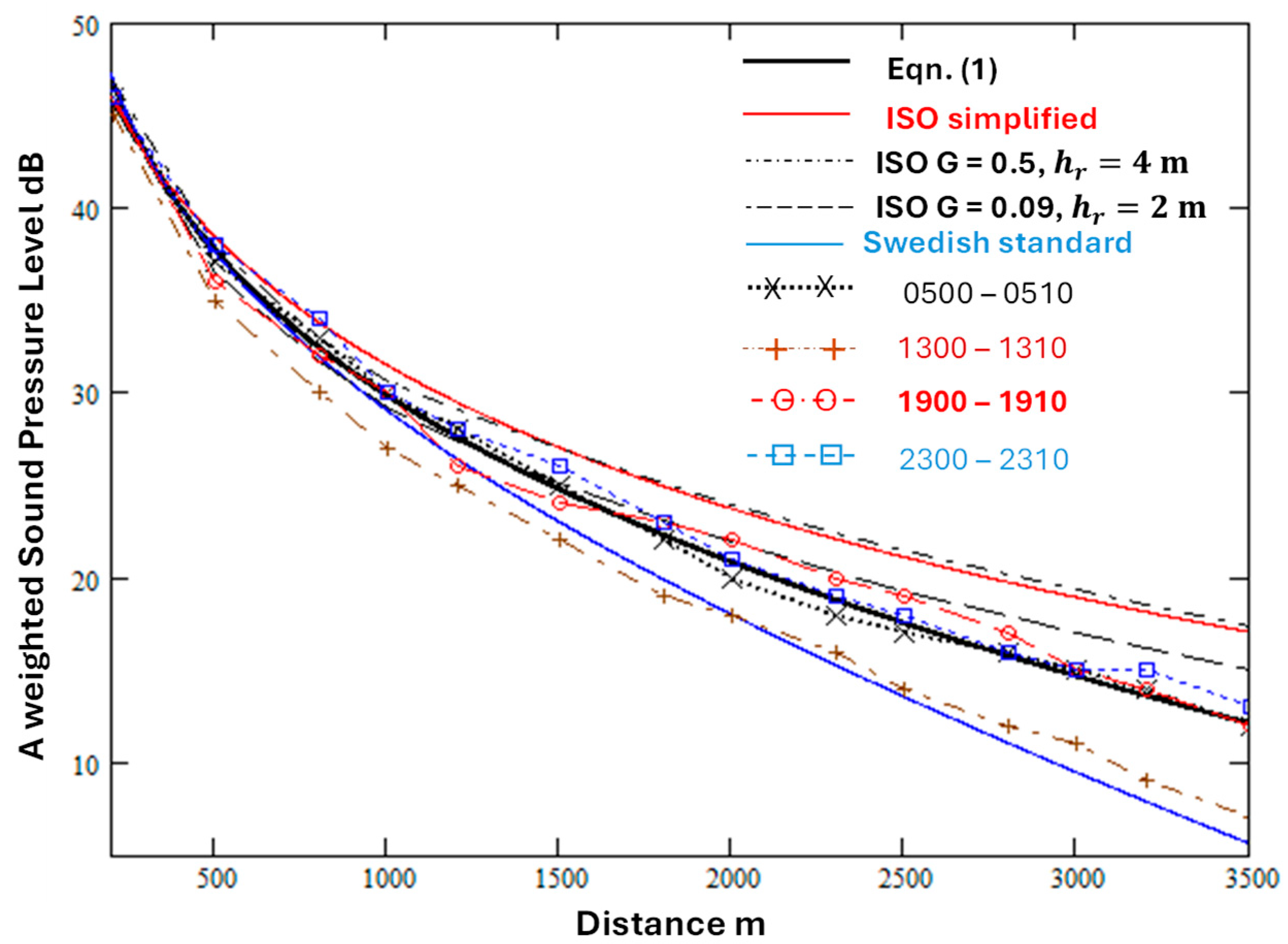
Barlas et al. [16] have investigated the diurnal variation of the A-weighted sound levels from a wind turbine using data obtained at 2 m high receivers in a validation exercise for the NORD2000 prediction scheme [17]. The measured average levels downwind over four 10-min periods at distances between 200 m and 3.5 km are shown in Figure 9 (from Figure 8 in [16]) together with predictions of Equations (1) and (2), the ISO9613-2 [1] octave band method and modified simplified method (Equation (7)) and the Swedish standard prediction (Equation (8)).

Figure 9. Average A-weighted sound levels measured at distances between 200 m and 3.5 km from a wind turbine over flat terrain [18] during four 10-min periods in a single day (joined points) compared with predictions of Equations (1) and (2) with ${\gamma }_g=0.0001$, ${\gamma }_t= {10}^{-6}$, ${\gamma }_R= -1\times {10}^{-6}$ (solid black line). Predictions of the Swedish scheme (solid blue line), the ISO9613-2 [1] octave band method ($G=0.5$, $h_r=4$ m—black dash dot line; $G=0.09$, $h_r=2$ m—broken black line) and the simplified method (solid red line) are shown also. Predictions of the octave band method use the sound power spectrum in Table 2. $L_{WA}$ = 102 dB matches the measured levels at 200 m.

The levels measured during the early morning (0500–0510 h), evening (1900–1910 h) and nighttime (2300–2310 h) are similar and are close to the predictions of Equations (1) and (2). The predictions of the ISO9613-2 [1] octave band method with $G=0.5$ and $h_r=4$ m and the modified simplified method (Equation (7)) are similar, and both tend to overestimate the levels beyond 500 m. The predictions of the ISO9613-2 [1] octave band method with $G=0.09$ and $h_r=2$ m are closer to the data for the early morning, evening and nighttime periods but not as close as the prediction of Equations (1) and (2). Beyond 1.5 km, the prediction of the Swedish scheme (Equation (8)) is close to the average levels measured during the early afternoon period (1300–1310 h). However, these are significantly lower than the levels during the other periods. Barlas et al. [16] attribute this to a difference in effective sound speed profile. Figure 2 in ref. [16] shows that the wind speed gradient and temperature lapse gradient below 100 m during this period are much steeper that during the other periods and imply a logarithmic sound speed profile rather than the linear one assumed by Equations (1) and (2).

Könecke et al. [18] have reported the difference between the sound levels measured by 1.7 m high receivers at two distances (535 m and 845 m) and the level measured at 178 m from a wind turbine (hub height 119 m, rotor length 57 m) over relatively flat grass covered ground during a variety of meteorological conditions. The meteorological measurements included relative humidity, pressure (at 57 m height), temperature, wind speed and wind direction (at heights of 28 m, 53 m and 95 m). Könecke et al. [18] compare their measurements with predictions using a numerical (PE) method which does not include turbulence. They represent the turbine noise source as three incoherent monopole sources located at hub height and at hub height ± 0.85 × rotor length and find that this enables better agreement with data than assuming a single monopole source at the hub height. The overall attenuation of $L_{pA}$ calculated from their third octave band level difference data between 80 Hz and 2 kHz for two (slightly) downwind conditions are compared with predictions of Equations (1), (2), (6) and (7) and the ISO octave band method in Table 3.

Table 3. Measured and predicted A-weighted sound level differences.

	Measured [18]	${\mathit{h}}_{\mathit{s}}$ m	Equations (1) and (2)	Equations (1) and (2) Sum	Equation (6)	Equation (7) Sum	ISO G = 0.5	ISO Sum	Equation (8)
level difference 178 m–535 m dB(A)	18.5	167.45	13.2	14.1	11.1	11.3	10.7	11.9	8.3
		119.00	13.9		10.2		10.7
		70.55	15.4		8.6		10.7
level difference 178 m–845 m dB(A)	24.8	167.45	19.8	21.1	14.7	15.6	15.5	16.7	16.9
		119.00	21.0		13.7		15.5
		70.55	23.6		12.7		15.5

Predictions of Equations (1), (2) and (6) and the ISO octave band method (with $G=0.5$, $h_r=4$ m) are for the three monopole heights (hub height and at hub height ± 0.85 × rotor length) considered by Könecke et al. [18]. The values in the columns headed ‘Sum’ are the level differences after summing the levels due to three incoherent sources at each of the heights in column 3 for each distance. A frequency independent value of $\alpha =5\times {10}^{-3}$ nepers per m (7.8 dB/km) has been used. for predictions with Equations (1) and (6). According to Figure 5b in Könecke et al. [18], this corresponds to a frequency near 1.5 kHz. The other parameter values used for Equations (1) and (2) predictions are ${\gamma }_g=0.0231$, ${\gamma }_t={10}^{-6}$ and ${\gamma }_R=-1\times {10}^{-6}$. From Equation (5), the value ${\gamma }_g=0.0231$ used Equations (1) and (2) predictions corresponds to $G=1$ but $G=0.5$ has been used for the ISO octave band predictions.

Könecke et al. [18] report that their numerical predictions for the propagation losses for the two light downwind cases are within 1 dB of those measured. Equations (1) and (2) predictions for the lowest height source are within 3.1 and 1.2 dB respectively of the measured level differences. The predictions of Equations (1) and (2) for the difference between the total levels after summing the contributions from incoherent sources at three assumed heights are within 4.4 dB and 3.7 dB respectively of the measured level differences. These predictions are closer to the measured level differences than those of the ISO9613-2 [1] simplified and octave band methods and the Swedish standard (Equation (8)). As well as being about 7 dB less than those measured for the summed contributions, the level differences predicted by the ISO octave band method with $G=0.5$ and $h_r=4$ m for the individual sources do not vary with the source height. The differences in the summed levels predicted by the ISO9613-2 [1] simplified method (7.2 and 9.2 dB respectively) are significantly less than the measured level differences. Moreover, the ISO simplified method predicts increases in level differences with increasing height of the individual sources which is not supported by the physics of ground effect.

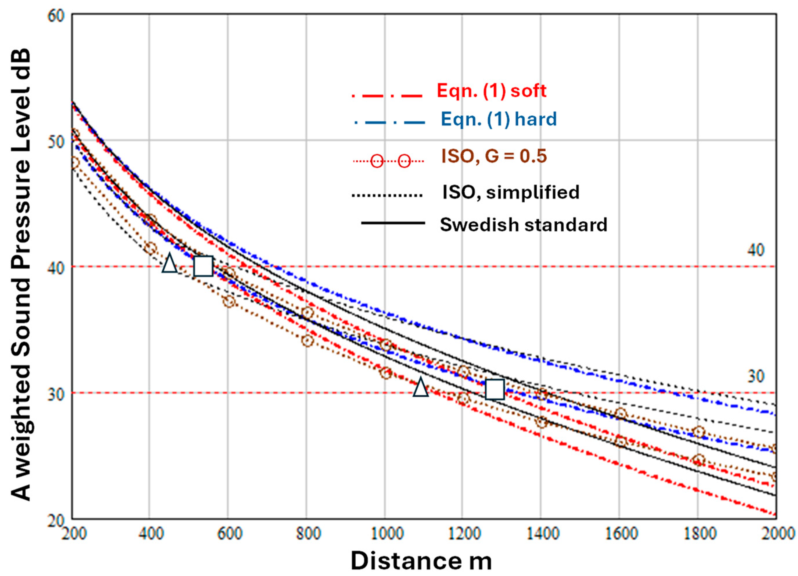
Van den Berg et al. [15] have compared turbines having blades with and without serrated edges. Another distinction is that between turbine spectra with a relatively high low frequency content and others. Van den Berg et al. [15] have used the ISO9613-2 [1] octave band method with $G=0.5$ to estimate the distances at which the overall A-weighted levels would be 40 dB(A) and 30 dB(A) for higher ($L_{WA}=108$ dB) and lower ($L_{WA}=105.8$ dB) sound power level wind turbines of between 3 and 6 MW power output without serrated edge blades (see Table 2 in [15]). These estimates are listed in Table 4. The higher source sound power level is associated with a turbine spectrum in which the low frequency content is relatively high, and the lower sound power level corresponds to a turbine spectrum with relatively little low frequency content [15]. Van den Berg et al. [15] mention immission heights of 1.5 m and 4 m without specifying which applies to their Table 2. An immission height of 1.5 m is assumed here.

Table 4. Estimates of distances at which levels of 30 and 40 dB(A) are reached predicted by the ISO9613-2 [1] octave band method with $G=0.5$ and $h_r=1.5$ m [15].

Sound Power Level dB(A)	Distance to 40 dB(A) m	Distance to 30 dB(A) m
105.8	430	1060
108	540	1280

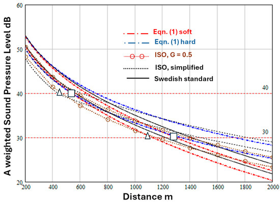
Figure 10 compares predictions of Equations (1), (2), (7) and (8) with these estimates. Turbine hub heights are not specified in Van den Berg et al. [15], so a hub height of 119 m has been assumed (corresponding to the turbine considered by Konecke et al. [18]). Predictions of Equations (1), (2) and (7) in Figure 8 assume $h_r=1.5$ m. For both the lower and higher power turbines, predictions of Equations (1) and (2) with ‘soft’ ground are closer to those estimated by using the ISO9613-2 [1] octave band method with $G=0.5$ and $h_r=4$ m than the predictions of the Swedish method (Equation (8)). The ISO simplified method predicts less attenuation than the ‘hard’ ground predictions of Equations (1) and (2), which, in turn, predict less attenuation for ‘hard’ than for ‘soft’ ground. Although the predictions of Equations (1) and (2) for ‘hard’ and ‘soft’ ground are similar at 500 m, significantly less attenuation is predicted for ‘hard’ ground beyond 1 km. The distances predicted by Equations (1) and (2) over ‘hard’ ground from the higher sound power level source at which levels of 40 dB(A) and 30 dB(A) are reached are 700 m and 1700 m respectively. The distances from the lower sound power level source predicted by Equations (1) and (2) are identical with the ISO octave band estimates with $G=0.5$ and $h_r=4$ m for the higher sound power level source.

Figure 10. Predictions variation of A-weighted sound level with distance according to Equations (1) and (2) for a source height of 65 m, receiver height of 1.5 m, $L_{WA}=108 \mathrm{or} 105.8$ dB, ${\gamma }_t={10}^{-6}$, ${\gamma }_R=-1\times {10}^{-6}$ (weak downward refraction), for two values of ${\gamma }_g=0.002$ and ${\gamma }_g=0.000001$ representative of acoustically ‘soft’ and ‘hard’ ground respectively. Also shown are predictions of the Swedish standard (continuous lines) and the ISO9613-2 [1] simplified method. The open squares and open triangles are estimates of the distances at which the levels obtained with the ISO9613-2 [1] octave band method (with $G=0.5$ and $h_r=4$ m) are 40 dB(A) and 30 dB(A) respectively for higher and lower power wind turbines without serrated edge blades (see Table 2 in [15]).

Barlas et al. [19] have modelled propagation from a US National Renewable Energy Laboratory 5 MW reference wind turbine (rotor diameter 126 m and hub height 90 m) and predicted downwind propagation to 2 m high receivers on flat grassland (effective flow resistivity 112.5 kPa s m⁻²) using the Parabolic Equation numerical method including turbulence and a 4-parameter ground impedance model. Their predictions are made for two values of ground roughness and two hub height wind speeds (see Table 5). Cases 1 and 2 correspond to higher temperatures and lower relative humidities than cases 3 and 4.

Table 5. Parameters used in predictions by Barlas et al. [19].

Case	Ground Roughness (m)	Hub Height Wind Speed (m s−1)
1	0.5	6
2	0.005	6
3	0.5	9
4	0.005	9

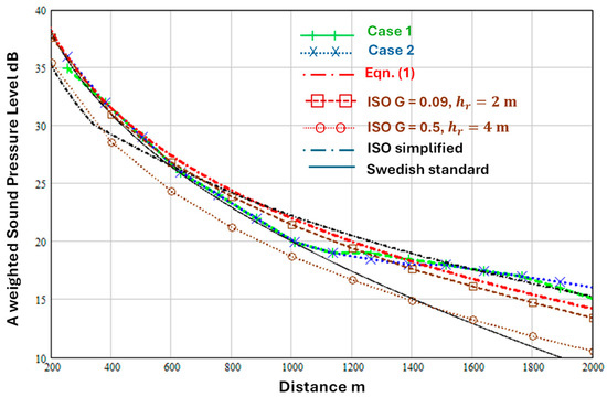
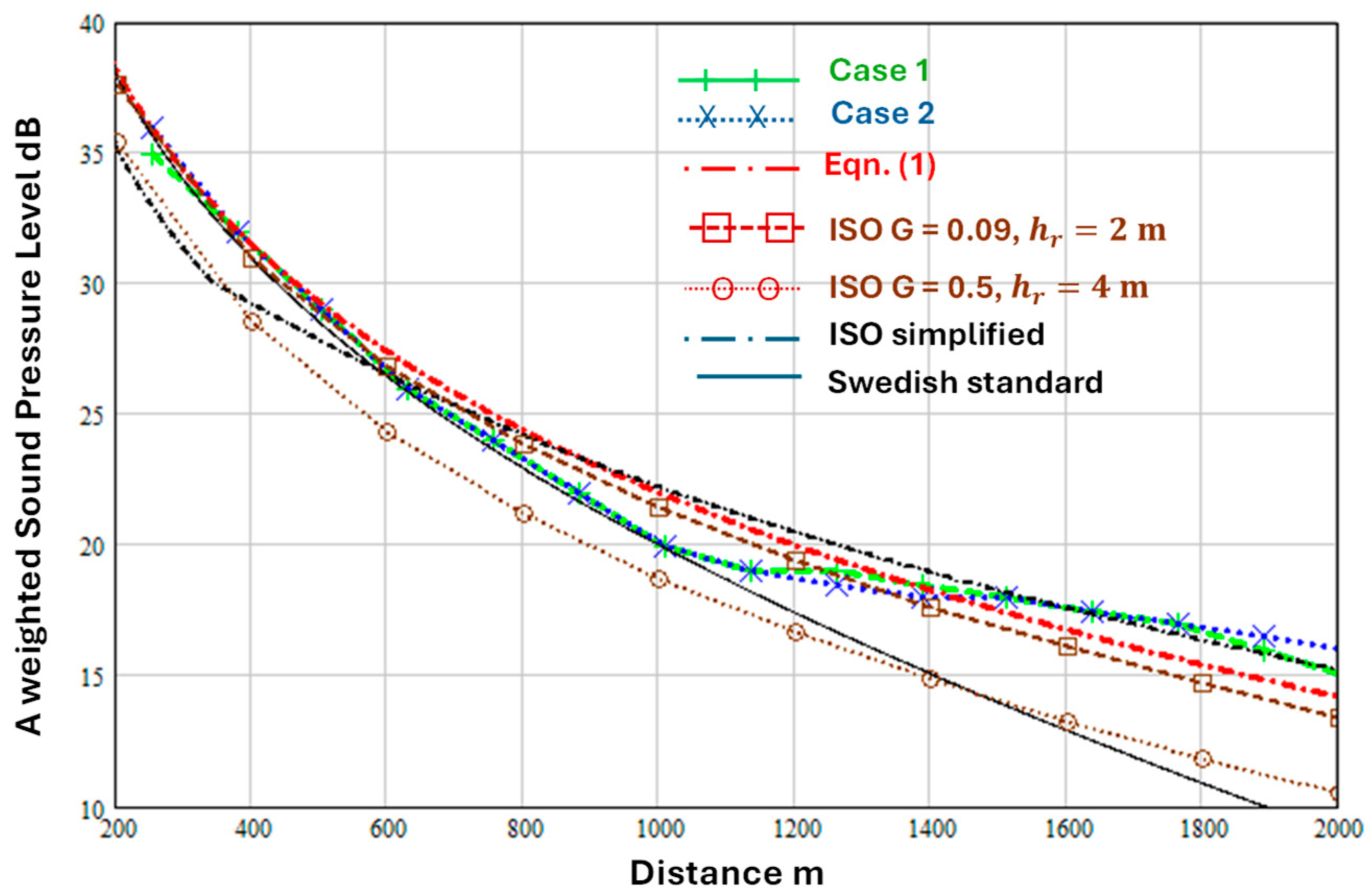
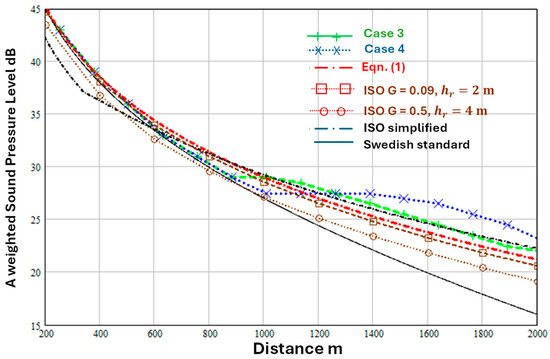
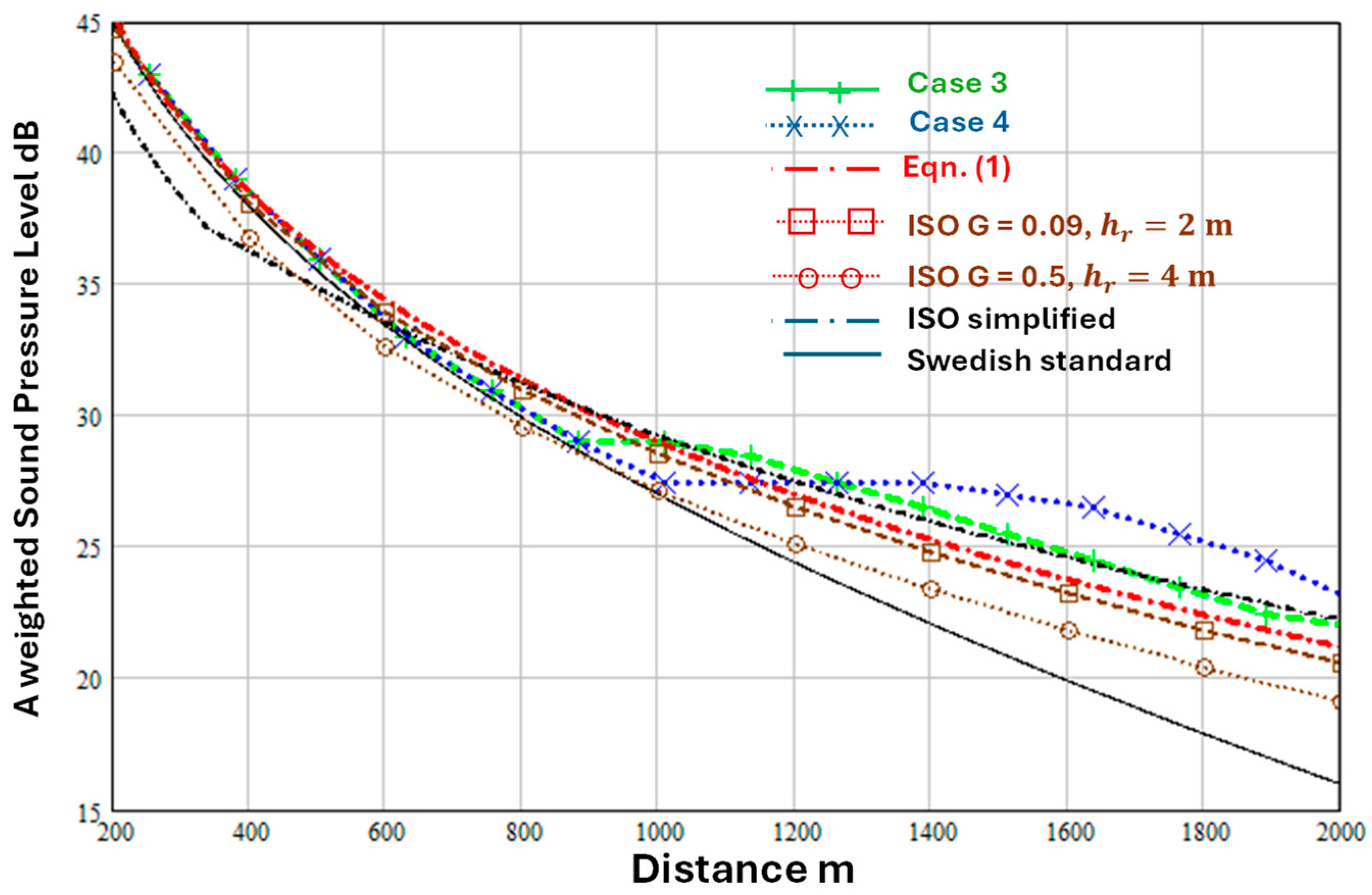
Figure 11 and Figure 12 compare the numerical predictions of Barlas et al. [19] with predictions of Equations (1), (2), (7) and (8) and the ISO9613-2 [1] octave band method.

Figure 11. Predicted variation of A-weighted sound level with distance (joined points) between 200 m and 2 km over flat grassland according to Barlas et al. [19] for a hub height of 90 m, receiver height of 1.5 m (a) for cases 1 and 2 (see Table 4). Also shown are predictions of Equations (1) and (2) (dash dot red line), the Swedish standard method (continuous black line) and the ISO9613-2 [1] octave band method for $G=0.09$ (joined open squares) and $G=0.5$ (joined open circles). The assumed A-weighted source sound power level is $L_{WA}=93$ dB and (b) $L_{WA}=100$ dB. Other parameter values used in the predictions with Equations (1) and (2) are ${\gamma }_g=0.00001$, ${\gamma }_t= {10}^{-5}$, ${\gamma }_R= -4\times {10}^{-6}$ (weak downward refraction) and $\alpha ={10}^{-5}$.

Figure 12. Predictions variation of A-weighted sound level with distance (joined points) between 200 m and 2 km over flat grassland according to Barlas et al. [17] for a hub height of 90 m, receiver height of 1.5 m for cases 3 and 4 (which involve higher wind speeds, see Table 4). Also shown are predictions of Equations (1) and (2) (dash dot red line) and the Swedish standard method (continuous line) and the ISO9613-2 [1] octave band method for $G=0.09$ (joined open squares) and $G=0.5$ (joined open circles). The assumed A-weighted source sound power level is $L_{WA}=100$ dB. Other parameter values used in the predictions with Equations (1) and (2) are ${\gamma }_g=0.00001$, ${\gamma }_t={10}^{-5}$, ${\gamma }_R=-4\times {10}^{-6}$ (stronger downward refraction) and $\alpha ={10}^{-5}$.

The 7 dB difference in the assumed source power levels used for Figure 11 and Figure 12 can be attributed to the difference in wind speeds [19]. According to Equation (5), the value of ${\gamma }_g=0.00001$ used in the predictions with Equations (1) and (2) corresponds to $G=0.09$. So, predictions of the ISO octave band method are shown for both $G=0.5$ ($h_r=4$ m) and $G=0.09$ ($h_r=2$ m).

For cases 1 and 2 [19] (Figure 11), Equations (1) and (2) and the ISO9613-2 [1] octave band method with $G=0.09$ and $h_r=2\mathrm{m}$ give predictions within ±2 dB of the numerical simulations up to 1 km and are within ±3 dB of the numerical results between 1 and 2 km. The predictions of Equations (1) and (2) and of ISO9613-2 [1] octave band method with $G=0.09$ and $h_r=2 \mathrm{m}$ are in close agreement for cases 3 and 4 (Figure 12) but predict between 2 and 4 dB lower levels than the numerical simulation for case 4 beyond 1300 m. Compared with the numerical simulations for cases 1 to 4, the ISO simplified method (Equation (6)) predicts levels that are 2 to 3 dB lower than numerical predictions out to 600 m but in close agreement beyond 600 m. The Swedish standard method (Equation (8)) gives predictions close to the numerical simulations for cases 1 to 4 out to 1 km but overpredicts the attenuation with distance beyond 1 km.

5. Conclusions

Measurements of outdoor sound propagation from loudspeakers, fixed jet engines and onshore wind turbines have been compared with various types of predictions including those of relatively accurate numerical methods and more approximate engineering methods. Although the simplified method for A-weighted sound levels from broadband sources in ISO9613-2 [1] is a practical engineering method, its predictions (a) do not agree with data over some ground surfaces, (b) do not change sufficiently rapidly with mean propagation path height and (c) for some cases (such as onshore wind turbines) suggest that the attenuation of downwind sound levels increases with source height, counter to the physics of ground effect.

The approximate analytical method (Equations (1) and (2)) is based on the physics of outdoor sound propagation and includes allowances for the type of soft ground, turbulence, atmospheric refraction, air absorption. Furthermore, it can be used where there is a single impedance discontinuity. The adjustable parameters introduced by the method can be fixed for representative situations based on comparing its predictions with data for source-receiver distances of up to 3.5 km. The approximate analytical method agrees better with the measured attenuation over ‘softer’ surfaces than does the ISO9613-2 [1] simplified method (modified to include air absorption) and predicts a more rapid decrease in ‘soft’ ground effect with source height. Consequently, the approximate analytical method (Equations (1) and (2)) is recommended as a potential replacement for the ISO9613-2 simplified method [1].

Predictions of the Swedish standard method for A-weighted levels from wind turbines (Equation (7)) have been shown to be close to those of Equations (1) and (2) for ‘very’ soft ground. However, Equations (1) and (2) and the ISO9613-2 [1] simplified method including a frequency independent air absorption (Equation (7)) give predictions in better agreement with data and numerical predictions than Equation (8) at distances of over 1 km where Equation (8) predicts too much attenuation.

When compared with measurements of wind turbine sound levels, where the actual receiver height is 2 m, the ISO9613-2 [1] octave band predictions can be improved by using $G=0.09$ and $h_r=2$ m rather than $h_r=4$ m as suggested in the standard. Nevertheless, the approximate analytical method, while requiring simpler calculations, gives predictions closer to data and numerical predictions than the ISO9613-2 [1] octave band method even with $G=0.09$ and $h_r=2$ m, which suggests that it could be considered as an alternative to the ISO octave band method also.

References

- ISO 9613-2:2024; Acoustics—Attenuation of Sound During Propagation Outdoors Part 2: Engineering Method for the Prediction of Sound Pressure Levels Outdoors. International Organization for Standardization: Geneva, Switzerland, 2024.
- Makarewicz, R. Industrial noise from a point source. J. Sound Vib. 1999, 220, 193–201. [Google Scholar] [CrossRef] [Scilit]
- Makarewicz, R.; Kokowski, P. Simplified model of ground effect. J. Acoust. Soc. Am. 1997, 101, 372–376. [Google Scholar] [CrossRef] [Scilit]
- Attenborough, K.; Van Renterghem, T. Predicting Outdoor Sound, 2nd ed.; CRC Press: Cambridge, UK, 2021. [Google Scholar]
- ESDU Data Item No. 940355; The Correction of Measured Noise Spectra for the Effects of Ground Reflection. ESDU International plc: London, UK, 1994.
- Parkin, P.H.; Scholes, W.E. The horizontal propagation of sound from a jet close to the ground at Hatfield. J. Sound Vib. 1965, 2, 353–374. [Google Scholar] [CrossRef] [Scilit]
- Zouboff, V.; Brunet, Y.; Berengier, M.; Sechet, E. A qualitative approach of atmospherical effects on long range sound propagation. In Proceedings of the 6th International Symposium on Long Range Sound Propagation; Havelock, D.I., Stinson, M., Eds.; National research Council of Canada (NRCC): Ottawa, ON, Canada, 1994; pp. 251–269. [Google Scholar]
- Attenborough, K.; Waters-Fuller, T.; Li, K.M.; Lines, J.A. Acoustical properties of farmland. J. Agric. Eng. Res. 2000, 76, 183–195. [Google Scholar] [CrossRef] [Scilit]
- Zaporozhets, O.; Tokarev, V.; Attenborough, K. Predicting Noise from Aircraft Operated on the Ground. Appl. Acoust. 2003, 64, 941–953. [Google Scholar] [CrossRef] [Scilit]
- Golebiewski, R. Simple methods for the determination of the acoustical properties of ground surfaces. Arch. Acoust. 2007, 32, 827–837. [Google Scholar]
- Department of Transport; Welsh Office. Calculation of Road Traffic Noise; HMSO: London, UK, 1988. [Google Scholar]
- Forssen, J.; Schiff, M.; Pedersen, E.; Persson Waye, K. Wind Turbine Noise Propagation over Flat Ground: Measurements and Predictions. Acta Acust. 2010, 96, 753–760. [Google Scholar] [CrossRef] [Scilit]
- Kragh, J.; Plovsing, B. Nord2000. Comprehensive Outdoor Sound Propagation Model; Part I–II.; DELTA Acoustics & Vibration Report 1849-1851/00; DELTA Acoustics & Vibration: Lyngby, Denmark, 2000; (Revised 31 December 2001). [Google Scholar]
- Swedish Environmental Protection Agency. Noise from Wind Turbines; Report 6241; Swedish Environmental Protection Agency: Stockholm, Sweden, 2001. (In Swedish) [Google Scholar]
- van den Berg, F.; Koppen, E.; Boon, J.; Ekelschot-Smink, M. Sound power of onshore wind turbines and its spectral distribution. Sound Vib. 2025, 59, 1716–1726. [Google Scholar] [CrossRef] [Scilit]
- Barlas, E.; Wu, K.L.; Zhu, W.J.; Porté-Agel, F.; Shen, W.Z. Variability of wind turbine noise over a diurnal cycle. Renew. Energy 2018, 126, 791–800. [Google Scholar] [CrossRef] [Scilit]
- Søndergaard, B.; Plovsing, B.; Sørensen, T. Validation of the NORD2000 Propagation Model for Use on Wind Turbine Noise; PSO-07 F&U Project (7389); Delta: Lyngby, Denmark, 2009; pp. 1–53. [Google Scholar]
- Könecke, S.; Hörmeyer, J.; Bohne, T.; Rolfe, R. A new base of wind turbine noise measurement data and its application for a systematic validation of sound propagation models. Wind. Energy Sci. 2023, 8, 639–659. [Google Scholar] [CrossRef] [Scilit]
- Barlas, E.; Zhu, J.W.; Shen, W.Z.; Dag, K.O.; Moriarty, P. Consistent modelling of wind turbine noise propagation from source to receiver. J. Acoust. Soc. Am. 2017, 142, 3297–3310. [Google Scholar] [CrossRef] [Scilit] [PubMed]
Disclaimer/Publisher’s Note: The statements, opinions and data contained in all publications are solely those of the individual author(s) and contributor(s) and not of MDPI and/or the editor(s). MDPI and/or the editor(s) disclaim responsibility for any injury to people or property resulting from any ideas, methods, instructions or products referred to in the content. |
© 2026 by the author. Licensee MDPI, Basel, Switzerland. This article is an open access article distributed under the terms and conditions of the Creative Commons Attribution (CC BY) license.