


Abstract
We compare direct and factorized prediction under an exactly known microbial multiplier and a multiplicative target law. The revised synthetic generator couples phase flow, velocity and holdup through a common pipe area and a prescribed slip closure. Across 30 draws, complete-pipeline holdouts yielded 7950 predictions, including 1879 active cases (23.6%). With the same exact factor supplied to both extreme gradient boosting (XGBoost) procedures, grouped active root-mean-square error (RMSE) was 0.06099 mm/year for direct learning and 0.04207 mm/year for factorized reconstruction. Inactive RMSE was 0.02951 and 0.02981 mm/year, respectively. Factorization had lower pooled RMSE in 29 of 30 grouped draws and 30 of 30 random splits. Shared factor errors could reverse the active-case ranking. Factorized Ridge had pooled RMSE of 0.03061 mm/year. In a separate AH36 laboratory study, the cell-mean reference had the lowest RMSE across 16 held-out treatment-replicate means.
1. Introduction
Internal corrosion assessment in gas gathering pipelines connects aqueous exposure, degradation mechanisms and inspection priorities. Sulfate-reducing bacteria (SRB) can contribute to microbiologically influenced corrosion (MIC) through sulfide production, biofilm activity, and access to electron donors [1]. Experiments on X80 pipeline steel further show that nutrient availability and sessile activity affect corrosion and mechanical deterioration [2]. Liquid-retention descriptors provide a useful basis for organizing exposure hypotheses alongside these biological processes.
Recent MIC reviews emphasize microbial attachment, community interactions, material properties and local electrochemical conditions [3]. These findings motivate separating a hydrodynamic exposure descriptor from the biological response represented by a microbial multiplier.
Liquid holdup describes a bulk hydrodynamic state governed by phase flow rates, flow pattern and inclination [4]. Experimental oil–water studies relate corrosion to aqueous wall contact [5], while surface wettability and intermittent exposure modify the distribution and duration of that contact [6,7]. We use holdup as an exposure proxy and prescribe its activation threshold to create a controlled numerical comparison of microbial correction strategies.
Electrochemical measurements combined with near-wall visualization show that pre-wetting and oil-film rupture affect corrosion initiation in oil–water flow [8]. This surface and temporal dependence motivates examining both abrupt and smooth activation functions in the benchmark.
Machine learning models have been used to predict internal corrosion from literature-derived descriptors [9] and from scenarios generated with OLI Studio [10]. These studies motivate nonlinear regression within an explicitly described data domain. For a correction-based model, the provenance of the target additionally determines whether a multiplier represents an omitted contribution or repeats a contribution already present in the training labels.
An independent machine-learning analysis using records from more than 35,000 condition-monitoring locations reports increasing uncertainty at higher corrosion rates [11]. This result motivates examining exposure-regime coverage alongside pooled fit metrics when assessing conditional correction.
Neural networks have incorporated physical constraints when predicting maximum pipeline pitting depth [12] and corrosion in subsea multiphase transport [13]. Hybrid models combine a learned component with prescribed structure [14]. Here, the training target determines where to place a prescribed multiplier. Applying it to a prediction of a rate that already includes the multiplier can count the same contribution twice.
We use extreme gradient boosting (XGBoost) for the primary comparison [15]. Random splits can give optimistic estimates for correlated observations [16]. To assess transfer to new pipelines, we withhold complete pipelines [17] and report errors separately for active and inactive test segments.
We ask how a prescribed multiplier affects prediction when it enters the training target, the direct inputs or reconstruction. We compare factorized reconstruction with direct regressors that receive the same factor, the 15 original covariates alone, or those covariates plus raw microbial descriptors. The nominal generator makes the factor recoverable from the original covariates. We therefore also simulate a separate microbial channel and test the procedures with shared factor errors. Post-multiplication of a total-rate prediction serves as a diagnostic for double application.
The synthetic experiments repeat the comparison across 30 draws and complete-pipeline holdouts. In a separate laboratory reanalysis, we estimate the factor from the training controls and predict held-out biological replicates. The fully interacted and saturated models show how much of the laboratory comparison depends on the form of the fitted model.
2. Materials and Methods
2.1. Synthetic Benchmark and Prescribed Factors
The computational benchmark uses synthetic segment records generated in Python with NumPy default_rng, with seeds 5001–5030 for the 30 repeated realizations. The sample comprises three artificial pipelines with 90, 90 and 85 segments at 10 m nominal chainage. Four independent latent sequences per pipeline follow the stationary first-order autoregressive (AR(1)) process in Equation (1), with coefficient 0.85, initial state z0~N(0,1) and independent standard-normal draws ηi:
The logistic transform σ(z) = 1/(1 + exp(−z)) maps latent variables to bounded scenario inputs. Table 1 defines the fifteen regression covariates. Each pipe has internal diameter D = 0.30 m and area A = πD2/4. Liquid density is 1000 kg/m3. Gas density is ρg = 106 P M/(Z R TK), with P in MPa, TK = T + 273.15 K, molar mass M = 0.018 kg/mol, compressibility Z = 0.90 and R = 8.314462618 J/(mol K). Gas volume is reported at the local operating pressure and temperature.
Table 1.
Regression covariates of the revised synthetic generator. Bars denote the mean of the latent sequence within a pipe. Phase flow rates, velocities and holdup share the same area and reference state.
At each pipe inlet, qg,0 = [1.49 + 4.24 σ()] × 104/86400 m3/s and P0 = 13.67 + 0.25 σ(z3,0) MPa. Liquid flow is ql = [471 + 1173 σ(0.7 + 0.3 )]/86400 m3/s. Gas mass flow ρg,0 qg,0 and liquid flow remain constant along each pipe. With slip S = ug/ul = 1 + 4 σ(z2), continuity gives HL = S vsl/(vsg + S vsl), ul = vsl/HL and ug = vsg/(1 − HL). Elevation is 3 sin(x/110 + 0.4 p) + 1.2 cos(x/45) + 0.5 z4 m at 10 m spacing. Pressure increments equal minus the trapezoidal friction and elevation losses, using ρm = HL ρl + (1 − HL)ρg and friction gradient fD ρm(vsg + vsl)2/(2D), with Darcy factor fD = 0.015. The supplied code solves this prescribed closure iteratively. The numerical microbial inputs remain N = 50 exp(1 + 0.8 z2) cells/mL and X = 15 + 100 σ(z4) mg/L.
The slip, bore, density and friction coefficients are fixed scenario settings. The gas and liquid shear covariates are proxies for fD ρg vsg2/8 and fD ρl vsl2/8. The supplement records the exact input scales for regularized and neural models. All prescribed seeds and folds were retained throughout the comparison.
Equation (2) defines the dimensionless microbial multiplier using the fixed scenario coefficients in Table 2. Experiments on microbial activity and nutrients motivate the choice of descriptors [1,2]. The coefficients and functional form specify a numerical benchmark. A raw factor F is clipped between one and three:
Table 2.
Fixed coefficients defining the numerical microbial-factor scenario.
Across the 30 revised draws, pressure ranges from 13.521 to 13.898 MPa, so the pressure term contributes 0.203–0.208 to the multiplier. It acts mainly as an offset. Equation (2) specifies the numerical microbial scenario. Section 2.4 checks the offset by centering and omitting the pressure term. The revised phase closure supplies consistent flow and holdup inputs without estimating microbial kinetics or biofilm transport.
The effective factor g(HL) equals fbac when HL > 0.1 and equals one otherwise; exact equality at HL = 0.1 belongs to the inactive branch. The threshold is fixed for the numerical benchmark. Surface wettability, aqueous-phase distribution and flow history motivate evaluating alternative exposure transitions [5,6,7]. The clean baseline rate b is assigned in mm/a using uT = (T − 18.5)/23.8, uCO2 = (PCO2 − 0.0420)/0.0004, uv = (vsg − 2.34)/8.73, uτ = (τg − 0.22)/3.17, upH = (5.84 − pH)/0.75 and d = clip(−θr/0.108, 0, 1):
Equation (3) defines the synthetic baseline with fixed coefficients in mm/a. The term p mod 3 is the remainder of the artificial pipeline identifier p divided by three and introduces a group offset; the identifier is excluded from the regression covariates. The total target y combines b with the prescribed factor and independent relative Gaussian noise ε of standard deviation 0.025, as in Equation (4). Here a denotes year. This construction supplies a known numerical reference for comparing correction procedures:
2.2. Information Sets and Prediction Procedures
Let x denote the fifteen covariates, y the generated total corrosion rate and g the exact effective scenario factor. In the matched comparison, a direct regressor learns y from (x, g), while a factorized regressor learns y/g from x and multiplies its output by g. Both procedures receive the same factor at training and prediction. With y = b g(1 + ε) and the exact generating g, the factorized learner sees b(1 + ε), with residual scale proportional to b. The direct fifteen-input model and the model supplied with additional N and X use the same targets and splits (Table 3).
Table 3.
Information and target definitions of the four primary synthetic extreme gradient boosting (XGBoost) procedures. The same scenario g is available to the two primary compared procedures.
The primary fixed-preset XGBoost comparisons use 400 trees, maximum depth 6, learning rate 0.05, row and column subsampling of 0.9, histogram construction, squared-error loss, random seed 42 and one thread [15]. Section 2.7 separately tunes tree count and depth. All 30 seeds and all outer folds use the revised generator. Adding columns changes the random column-subsampling path, so each contrast compares complete fitted procedures under the stated settings.
For diagnostic negative controls, the direct fifteen-input total-rate prediction is multiplied globally by fbac or conditionally by g. Because y already contains the contribution, these controls repeat it. Supplementary Information reports these diagnostics and the random forest [18], backpropagation multilayer perceptron (BP-MLP) [19] and support vector regression (SVR) [20] comparisons. Synthetic Ridge, BP-MLP and SVR use prespecified feature-unit scales with training-only centering [21]. The scales in Table S16 avoid amplifying nearly constant training-pipe fluxes. BP-MLP and SVR also standardize the training target. Ridge retains alpha = 1 without tuning.
Mean squared error (MSE), mean absolute error (MAE), root-mean-square error (RMSE), coefficient of determination (R2) and mean absolute percentage error (MAPE) are calculated from exported row-level predictions. MSE has units (mm/a)2; MAE and RMSE have units mm/a; R2 is dimensionless and MAPE is a percentage. All generated targets are positive. Metrics are reported with subset counts. Within each subset, R2 compares squared error with the error of a constant equal to that subset’s target mean; negative values indicate larger error than this descriptive reference. This reference uses evaluation labels and is not a trained operational baseline. RMSE estimates, differences and interval endpoints are reported to four significant figures; calculations retain full numerical precision.
2.3. Repeated Evaluation and Exposure Diagnostics
Each of the 30 realizations contains 265 segments in three artificial pipelines of sizes 90, 90 and 85. A 212/53 random split uses split seed 42. Complete-pipeline evaluation separately withholds each pipeline and trains on the other two [17,22], giving training sizes of 175 or 180. All four procedures are refitted independently for every split. The three grouped prediction folds are combined within each realization. The dataset contains 7950 unique synthetic rows, reused to produce 1590 random-test and 7950 grouped predictions per procedure. The two evaluation protocols are summarized separately.
The primary transfer assessment withholds complete pipelines. Adjacent segments share autocorrelated latent inputs, so random row splitting describes interpolation within the sampled pipelines and can be optimistic for transfer [16,17]. Random splits are suitable for a within-pipeline interpolation objective only when the dependence and the intended prediction access are reflected in the validation design. Spatial blocks or time-separated records are preferable for prediction across reaches or inspection dates. The protocols reuse observations within each realization and are summarized separately. Active and inactive RMSE are reported first, with pooled RMSE as a secondary summary.
The independent generator draw is the paired unit. We combine the three group folds within each draw before comparing RMSE, because those folds have overlapping training data. We report direct-minus-factorized differences, two-sided exact sign tests, and distribution-free median intervals from paired order statistics with at least 95% binomial coverage. Absolute differences of at most 10−10 mm/year count as ties and are excluded from sign tests. Empty active subsets are retained in coverage counts and omitted from active-only paired summaries. Factor-range diagnostics record active test points outside the training g range. These checks measure marginal coverage, while multivariate support requires additional diagnostics.
2.4. Sensitivity and Distribution Challenges
The original frozen-factor grid varies the prediction-stage threshold (0.05, 0.075, 0.10, 0.125 and 0.15) and the scale of excess factor (0.5, 1.0 and 1.5). Above the selected threshold, the reconstruction factor is 1 + scale × (fbac − 1). The original targets and training factor stay fixed. This one-arm grid measures sensitivity of the reconstruction step. Section 2.7 describes the matched two-arm factor perturbation.
A separate generative sensitivity varies one assumption at a time: wN = 0.11 or 0.33, wP = 0.0075 or 0.0225 MPa−1, and H* = 0.05 or 0.15. The same 30 revised covariate/noise draws are retained. Targets are regenerated, and models refitted on all ninety group folds. Each four-strategy comparison uses identical evaluation rows and its own scenario factor.
The pressure sensitivity either omits the pressure term or replaces it with 0.00375 max [0,(P − 13.67 MPa)/(0.25 MPa)], equivalent to 0.015 MPa−1 max(0,P − 13.67 MPa). The reference pressure and interval match the inlet settings. For smooth activation, gδ = 1 + sδ(HL)(fbac − 1), where sδ(HL) = {1 + exp[−(HL − 0.1)/δ]}−1 and δ is 0.005 or 0.020. At finite HL, the logistic weight lies strictly between zero and one. Each scenario regenerates targets and refits both procedures under the same grouped protocol.
We also fit BP-MLP and Ridge on the nominal grouped splits. A separate 200-row distribution challenge uses four additional pipes with slip fixed at S = 1 for two pipes and S = 8 for two pipes. Phase density, pressure, velocity, holdup and targets are recomputed jointly. The development models are frozen for this test. The supplement reports the resulting active and inactive errors and all learner comparisons.
2.5. Open Experimental Calibration Case
Independent measurements were obtained from the open study of Ivanovich et al. [23] and the raw workbooks linked in its data-availability statement. We extracted the authors’ corrosion-rate values from Weight loss.xlsx using explicit worksheet and cell identifiers. The experiment exposed AH36 carbon steel to sterile medium or Pseudodesulfovibrio profundus at 0.1 or 30 MPa, under static or continuous-flow conditions, for 240 h. Each of the eight treatment conditions has two independent biological replicates and two mass-loss coupons per replicate: sixteen treatment-replicate units and 32 coupons. Triplicate balance readings are measurement repeats, not additional experimental units.
The empirical factor is calibrated from condition-matched controls. For context c = (pressure, flow category), let μB,c and μA,c denote mean biotic and sterile rates in the training replicate. We define fE,c = μB,c/μA,c and gE,c(B) = 1 + B(fE,c − 1), where B records the observed inoculation treatment. The experimental factor is estimated anew from measured controls; Equation (2), its cap and the holdup threshold belong to the separate synthetic branch. Numerical flow values differ between source descriptions, so we retain the reported static/flow categories. We preserve the authors’ reported rates and units, with the source-cell extraction and cache/formula audit supplied in the supplement.
We train on biological replicate R1 and test on R2, then reverse the split. Each training or test set contains eight treatment-replicate units and sixteen coupons. We estimate the factor and fit each model with training measurements. Direct models use pressure, flow category and inoculation. Factorized models fit y/gE using pressure and flow, then multiply by the training-calibrated gE. The cell means, XGBoost preset and training-scaled Ridge fit are fixed within this protocol.
To separate reconstruction from model structure, a second direct Ridge design includes all seven factorial contrasts of pressure, flow and inoculation, including their three-way interaction. Its factorized baseline includes pressure, flow and their interaction. Contrasts are effect-coded −1/+1; Ridge retains alpha = 1, an unpenalized intercept and training-only input/target standardization. Complete direct and factorized ordinary-least-squares (OLS) designs supply an unpenalized saturation check. These designs span all eight treatment means; equal nominal Ridge penalties do not imply invariant regularization after target transformation.
Each held-out treatment-replicate unit contains two coupons, which remain together in every split. Primary case-level reporting averages their observed and predicted rates before scoring the sixteen unit means; coupon-level metrics on all 32 observations are also reported. Both reporting levels describe biological-repeat prediction at the four observed pressure–flow contexts. The experimental case evaluates its training-calibrated microbial contrasts, while the fifteen-input pipeline model, its HL threshold and its concentration equation are evaluated in the synthetic branch.
2.6. Reproducibility
The corrected simulations used Python 3.12.14, NumPy 2.5.4, pandas 3.0.1, SciPy 1.18.1, scikit-learn 1.9.1, XGBoost 3.4.1 and Matplotlib 3.11.2. The revised package supplies the version 3 generator, fixed feature scales, split identities, phase-consistency checks, predictions and figure scripts. All synthetic results in the revised article and supplement were recalculated with that generator. Gain and Shapley attributions [24,25,26,27] and ordinal examples are supplied in the supplement.
OpenAI Codex assisted literature review, analysis planning, manuscript drafting and code preparation. Reported values were computed by executing the supplied scripts.
2.7. Factor Identifiability Uncertainty and Baseline Controls
The revised generator also makes g recoverable from x. The phase quantities give S = HL vsg/[(1 − HL)vsl], so z2 = logit[(S − 1)/4]. The H2S transform gives σ(z4). Together with observed pH, pressure and HL, these values reproduce N, X and g. We additionally generated independent AR(1) microbial inputs with the same coefficient and marginal transforms while holding the revised flow inputs, activation, clean rate and noise fixed. The three procedures use x alone, (x, g), or factorized reconstruction with the new exact g.
For shared uncertainty, we retained the nominal targets and gave both XGBoost procedures the same perturbed factor . Active rows were multiplied by 1 + δs, with δ = 0.10 or 0.20 and independent equiprobable signs s = ±1. Inactive rows retained = 1. The signs were fixed per row across the grouped folds and magnitudes. In the frozen comparison, only test inputs or reconstruction use . In the refitted comparison, the direct input and the factorized training divisor both use the same on training rows. Reconstruction uses the corresponding test . These are sensitivity scenarios with known activation and stipulated relative errors.
Alternative grouped controls use Ridge (alpha = 1) with the same g and the fixed scales in Table S16, XGBoost with a direct log target, a log offset with target log(y/g), and an additive residual target y − c(g − 1), with c equal to the median of training y/g. Predictions restore the corresponding offset or residual adjustment once. The two log models exponentiate predictions without a smearing correction. XGBoost is also tuned over (80 trees, depth 2), (160, 3) and (400, 6). Each arm selects the lowest total-rate squared error across two inner pipeline holdouts restricted to the outer training data. All comparisons use the same outer folds.
3. Results
3.1. Repeated Prediction with Controlled Factor Information
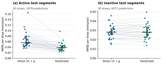
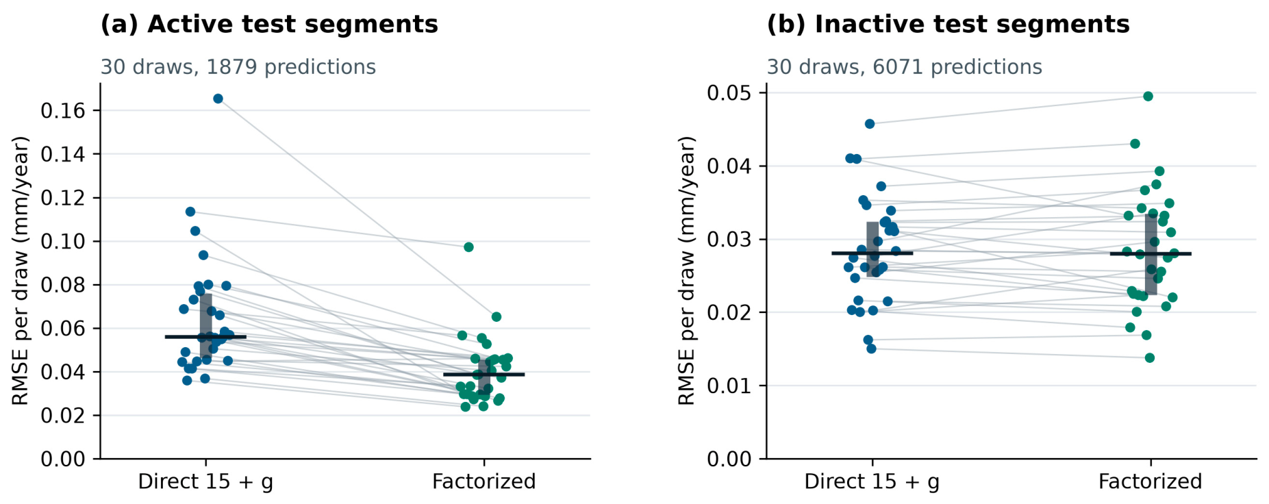
In complete-pipeline holdouts, 1879 of 7950 predictions (23.6%) were active. With the same exact factor supplied to both XGBoost procedures, grouped active root-mean-square error (RMSE) was 0.06099 mm/year for direct learning and 0.04207 mm/year for factorized reconstruction. Inactive RMSE was 0.02951 and 0.02981 mm/year, respectively. Pooled RMSE was 0.03930 and 0.03312 mm/year. Active cases contributed 3.6639 (mm/year)2 to the reduction in summed squared error, while inactive cases contributed −0.1062; the net reduction was 3.5576. The pooled random tests contain 394 active and 1196 inactive predictions; their results are reported separately in Table 4.
Table 4.
Fixed-preset XGBoost root-mean-square error (RMSE) (mm/year) by protocol and exposure subset. Counts are held-out predictions per procedure. Both Direct 15 + g and Factorized receive the exact generating factor.
Across the 30 grouped draws, factorized active RMSE was lower in 29 and higher in 1. The median paired reduction was 0.01768 mm/year (95.7% interval 0.01208–0.02708, exact two-sided sign p = 5.77 × 10⁻⁸). For all grouped rows, the median reduction was 0.005691 mm/year (95.7% interval 0.004617–0.006731, p = 5.77 × 10⁻⁸, 29 of 30). Factorization had lower pooled random RMSE in 30 of 30 draws (Table 5 and Table S12). Figure 1 separates the two grouped exposure strata. These tests quantify variability across draws from the revised generator.
Table 5.
Paired realization summaries for direct 15 + g versus factorized reconstruction. Lower/higher counts refer to factorized RMSE; n is the number of draws. Δ is direct minus factorized RMSE (mm/a). No ties occur.
Figure 1.
Paired complete-pipeline root-mean-square error (RMSE) with the same exact factor supplied to XGBoost procedures. Panel (a) shows 1879 active predictions and panel (b) 6071 inactive predictions, each across 30 draws. Each line joins a draw’s two RMSEs after combining the three grouped folds. Thick vertical bars and horizontal marks show interquartile ranges and medians. The panels use separate vertical scales. XGBoost is extreme gradient boosting.
The grouped median pooled reduction of 0.005691 mm/year is smaller than the spacing among the illustrative corrosion-rate boundaries of 0.025, 0.13 and 0.25 mm/year. Both procedures assigned all 7950 grouped rows to the same bands as their generated targets (Table S12). All generated rates lie above the highest boundary, giving identical band assignments for the two procedures. Evaluation for an intended application uses decision thresholds defined for that setting.
3.2. Exposure, Sensitivity and Learner Dependence
All ninety grouped training folds contain active observations. In grouped tests, 138 of 1879 active factors (7.3%) lie outside the training g range. Random tests contain 12 of 394 such cases (3.0%). Known-factor reconstruction imposes the prescribed multiplier at these values, while direct trees continue fitted leaf responses. Marginal range checks locate one aspect of the support difference.
The one-arm prediction-stage grid in Table S7 changes factorized RMSE from 0.03312 mm/year at the nominal threshold to 0.1417 at 0.05 and 0.1022 at 0.15. Its training factor and targets stay fixed. Section 3.4 compares both procedures under the same factor uncertainty.
Table S9 retains all eleven regenerated factor and gate scenarios. Each row compares the same four procedures on 7950 held-out predictions from the revised flow generator. Centering or removing the pressure term examines its reference offset, and smooth gates examine transition width. The main matched-information comparison remains Direct 15 + g versus factorized reconstruction.
Table 6 compares learners on active test rows from the nominal generator. Two subsets screen test rows against the training ranges, first for HL and then for all fifteen covariates individually. Above the nominal threshold, g = fbac, so the global and gated post-multiplication predictions coincide.
Table 6.
Active grouped RMSE (mm/a) by learner and marginal training range. BP-MLP is a backpropagation multilayer perceptron. The “15 ranges” subset checks each covariate individually. Global and gated columns show the two double-multiplication controls.
On all active rows, Direct 15 BP-MLP and Ridge gave RMSE of 0.1258 and 0.1114 mm/year, compared with 0.06820 for XGBoost (Table 6). The corresponding factorized values were 0.03214, 0.03959 and 0.04207. Section 3.4 adds direct Ridge with the same factor and compares results by factor support.
The revised fixed-seed random test has 2 active cases, and the pipeline-3 holdout has 24 (Tables S2 and S3). Table S4 reports the separate slip-distribution challenge, with 100 active and 100 inactive rows. All synthetic diagnostics were recalculated with the common-area generator.
3.3. Training-Calibrated Experimental Case
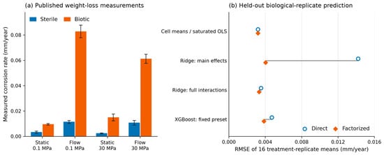
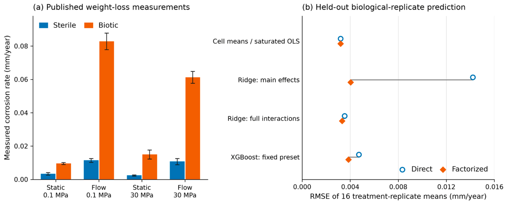
The measured biotic-to-sterile mean ratios are 2.8628 and 7.2886 at 0.1 MPa under static and flow conditions, and 6.3423 and 5.7376 at 30 MPa (Table 7). Three of the four ratios exceed the synthetic cap of 3.0. The observed contrasts apply to the tested AH36 conditions and motivate a separate calibration from the measured sterile and inoculated treatments.
Table 7.
Author-calculated summaries of corrosion rates extracted from the open weight-loss workbook linked by Ivanovich et al. [23]. Values are mean ± sample SD in mm/year across four coupons per treatment, nested within two biological replicates. Each ratio divides the biotic by the sterile mean in the corresponding context.
The cell-mean reference had the lowest RMSE on the sixteen held-out treatment-replicate means, at 0.003194 mm/year. Direct and factorized XGBoost gave 0.004723 and 0.003856 mm/year, respectively, and the Ridge errors were also higher than the reference (Table 8). Saturated OLS matched the cell means to numerical precision. The equality follows from the calibration: dividing the training biotic mean by the biotic-to-sterile ratio gives the sterile mean. Multiplying by that ratio recovers the biotic mean.
Table 8.
Descriptive experimental RMSE (mm/a) at both reporting levels. Unit means average two coupons within each of 16 held-out treatment-replicate units. OLS, ordinary least squares; saturated OLS matches the condition-mean reference.
Adding complete treatment interactions to direct Ridge changes unit-mean RMSE from 0.01420 to 0.003527 mm/a; the corresponding factorized interaction model gives 0.003320 mm/a. The large main effects contrast therefore includes interaction information supplied through the calibrated context factors. With all treatment interactions included, the remaining regularized-model difference also reflects the penalty coordinates. Figure 2 presents the measured contrasts and unit-level prediction errors. Coupon results, all fold-level predictions and the post-multiplication diagnostic controls remain available in the supplement.
Figure 2.
Author-generated plot from reanalysis of the open weight-loss workbook linked by Ivanovich et al. [23]. Panel (a) shows measured AH36 coupon means and sample SD from four coupons per treatment across two biological replicates. Panel (b) shows RMSE of sixteen held-out treatment-replicate means. Calibration uses the training replicate at each pressure–flow context. The cell-mean reference and saturated OLS give the same predictions.
3.4. Matched Factor Perturbations and Alternative Baselines
The nominal g was recovered from the revised fifteen inputs to a maximum absolute error of 4.4 × 10⁻¹⁶. With independent microbial inputs, active grouped RMSE was 0.07096 for Direct 15, 0.06705 for Direct 15 + g and 0.04012 mm/year for factorized reconstruction (Table S14). The comparison separates factor access from imposing the known product.
With frozen fits and shared ±10% and ±20% factor errors, direct active RMSE was 0.08455 and 0.08582 mm/year, while factorized RMSE was 0.07227 and 0.1242. With refitting, the direct values were 0.06731 and 0.06731, and the factorized values were 0.07627 and 0.1391 (Table S13). The ±20% frozen comparison and both refitted comparisons reverse the nominal active-case ranking.
Direct and factorized Ridge models with the same factor gave active RMSEs of 0.07225 and 0.03959 mm/year and pooled RMSEs of 0.04535 and 0.03061. Tuned direct and factorized XGBoost had active RMSE of 0.06166 and 0.04166. The log offset, direct log target and additive residual gave active RMSE of 0.04190, 0.06821 and 0.04754 mm/year (Table S14). Table S15 separates Ridge errors within and outside the training g range.
4. Discussion
4.1. Information Access and Structural Reconstruction
The total target already includes the microbial multiplier. A direct prediction that recovers b g would become proportional to b g2 after a second multiplication by g. We use this case to check for double application. The factorized procedure instead fits the baseline and multiplies its prediction by g. On the log scale, the corresponding offset is log g, since log y = log g + log b + log(1 + ε).
The revised nominal factor remains recoverable from the original inputs. Supplying g therefore gives the direct model a convenient representation of known input information. With independently generated microbial inputs, the direct tree’s active RMSE changed from 0.07096 to 0.06705 mm/year after adding g, while factorized reconstruction gave 0.04012. These comparisons concern the specified generator and learners.
Ridge uses the same scenario feature scales in both arms. Fitting y/g weights squared total-rate residuals by 1/g2 for a given reconstructed function. The direct and factorized forms also penalize coefficients in different bases. Table S15 locates the error differences by factor support. The comparison assesses their combined effect because weighting, basis and support vary together.
4.2. Calibration and Evaluation Domains
The revised generator enforces a common pipe area, constant phase mass flow, a prescribed slip relation and a discrete pressure balance. Across 7950 nominal rows, liquid phase velocity is 1.183–6.846 m/s and gas phase velocity is 4.729–8.319 m/s. Phase-flow residuals are below 10−12 m3/s. The closure uses fixed compressibility and friction parameters and omits acceleration losses. It defines the synthetic operating domain. Calibration of the microbial multiplier and the HL = 0.1 exposure threshold would require independent wall-contact, microbial and corrosion measurements. The AH36 case evaluates measured sterile/biotic contrasts between biological replicates at the same experimental settings.
Each treatment contributes two biological replicates. Both coupons within a replicate stay together when we split the data. The observed ratios and the synthetic cap apply to different quantities: the laboratory estimates compare inoculated and sterile conditions, while the cap bounds a multiplier specified by the pipeline generator.
The supplementary network and repeat-inspection examples apply an ordinal rule to synthetic rates. Their class supports are reported because the generated distributions are strongly imbalanced. Risk matrices summarize severity categories [28]. Asset integrity decisions additionally require corrosion-growth, defect-distribution and asset-specific information [29].
4.3. Evaluation Checklist
- Define the prediction target and units. Record whether the measured or generated labels contain the microbial contribution and whether the intended prediction is total corrosion or a baseline rate.
- Document the factor and how it is obtained at prediction time. Record whether it is specified, measured, estimated from training controls or reconstructible from other inputs. Keep calibration inside each training split and test shared factor errors when relevant.
- Quantify exposure coverage. Report active and inactive counts, folds without active training data and the share of active test factors outside training support. Record the gate and the uncertainty in its definition.
- Match the split to deployment. Withhold complete assets for transfer to new assets. Use spatial or temporal blocks for transfer across reaches or inspection dates. Keep coupons from the same replicate together and assess matched-context performance separately.
- Report active and inactive errors before pooled metrics. Include counts, paired effects at the independent-unit level, and direct and simple regularized baselines with comparable factor access. Evaluate decision thresholds separately when they govern an application.
5. Conclusions
Under the revised synthetic flow closure, an exactly known multiplier and a multiplicative target law, factorized XGBoost gave grouped active RMSE of 0.04207 mm/year, compared with 0.06099 for Direct 15 + g. Active cases represented 23.6% of the grouped predictions. Inactive RMSE was 0.02981 and 0.02951, respectively. Factorization had lower pooled error in 29 of 30 grouped draws and 30 of 30 random splits. Shared factor errors could reverse the active-case ranking. The alternative learners and transformed-target models show that performance depends on the fitted procedure and factor quality.
For AH36, the cell-mean reference gave the lowest error on biological replicates held out at the tested pressure and flow settings. The evaluation checklist in Section 4.3 links the prediction target, factor calibration and exposure coverage to the split and error metrics. Applying it to field pipelines would start with independent corrosion, wall-contact and microbial records.
Supplementary Materials
The following supporting information can be downloaded at: https://www.mdpi.com/article/10.3390/cmd7040083/s1. Figure S1: Response surface of the prescribed microbial factor in main Equation (2) at pH = 5.46 and P = 13.75 MPa; Figure S2: Computed RMSE and R2 of the four regressors on the simulated random test, n = 53; Figure S3: Predictions versus generated target rates for XGBoost, random forest, BP-MLP, and SVR on the same 53 simulated test rows; Figure S4: Recalculated correction errors on the revised random test; Figure S5: XGBoost errors on the slip-distribution challenge, with 100 inactive and 100 active cases; Figure S6: Normalized gain importance of the direct-target XGBoost model trained on simulated data; Figure S7: Native TreeSHAP contributions for the simulated direct-target model, showing the ten largest mean absolute contributions on the 53 test rows; Figure S8: Complete illustrative ordinal matrix; Figure S9: Class counts and percentages for 15,154 synthetic network segments; Figure S10: Confusion matrix for 487 revised synthetic repeat-inspection records; Figure S11: Author-generated plot from the open weight-loss workbook linked by Ivanovich et al.; Table S1: Computed baseline performance on generated targets, n = 53; Table S2: Correction procedures on the revised 53-row random test, including 2 active rows; Table S3: Fixed-seed results for artificial pipeline 3; Table S4: RMSE in mm/year and dimensionless R2 under the jointly generated slip challenge; Table S5: Pooled RMSE in mm/year across thirty revised generator draws; Table S6: Distribution of realization-level RMSE (mm/a) over thirty independent generator draws; Table S7: Pooled pipeline-holdout RMSE in mm/a under prediction-stage perturbations; Table S8: Out-of-replicate experimental RMSE (mm/a) for all learners and strategies, n = 32 coupon predictions; Table S9: Pooled XGBoost group-holdout RMSE (mm/a) after regenerating each scenario and refitting the models; Table S10: Exact class boundaries for the illustrative ordinal screening matrix; Table S11: Class support and recall on simulated repeat-inspection records; Table S12: Paired direct-minus-factorized RMSE by independent generator draw and counts of wrong-band assignments; Table S13: Shared factor perturbations on grouped holdouts; Table S14: Grouped RMSE for the revised nominal and independent microbial-channel generators; Table S15: Same-factor Ridge RMSE for active cases by marginal factor coverage; Table S16: Fixed feature divisors for synthetic Ridge, BP-MLP and SVR. The accompanying data and code package contains the revised generator, extracted laboratory data, predictions, analyses and figure scripts. References cited in the Supplementary Materials are included in the main reference list [17,22,23,24,25,26,27,28,29].
Author Contributions
Conceptualization, F.Z., Z.Z. and G.H.; methodology, X.L. and R.L.; software, X.L. and Y.Z.; validation, R.L. and Y.Z.; formal analysis, X.L. and R.L.; visualization, R.L. and Y.Z.; writing—original draft preparation, X.L., R.L. and Y.Z.; writing—review and editing, F.Z., Z.Z. and G.H.; supervision, G.H. All authors have read and agreed to the published version of the manuscript.
Funding
This research received no external funding.
Data Availability Statement
The corrected synthetic generator, all revised predictions and source-linked laboratory extraction accompany the manuscript. Experimental source workbooks are linked from Ivanovich et al. [23] at https://github.com/NicoloIvanovich/Exploring-the-impact-of-flow-dynamics-in-deep-sea-corrosive-biofilms (accessed on 17 November 2026). Extraction records preserve worksheet/cell identifiers and original values. The authors’ raw workbooks remain available from that source; this supplement supplies the derived tables and analysis code.
Acknowledgments
We thank Ivanovich and coauthors for sharing their experimental data. OpenAI Codex (OpenAI; accessed 1–2 November 2026) provided the assistance described in Methods. The authors are responsible for the final content.
Conflicts of Interest
Authors Fei Zhao and Zhao Zhang are employed by Chengdu Branch, China Petroleum Planning & Engineering Institute, PetroChina. The remaining authors declare that the research was conducted without any commercial or financial relationships that could be construed as a potential conflict of interest.
References
- Enning, D.; Garrelfs, J. Corrosion of iron by sulfate-reducing bacteria: New views of an old problem. Appl. Environ. Microbiol. 2014, 80, 1226–1236. [Google Scholar] [CrossRef] [Scilit] [PubMed]
- Li, Z.; Yang, J.; Guo, H.; Kumseranee, S.; Punpruk, S.; Mohamed, M.E.; Saleh, M.A.; Gu, T. Carbon Source Starvation of a Sulfate-Reducing Bacterium–Elevated MIC Deterioration of Tensile Strength and Strain of X80 Pipeline Steel. Front. Mater. 2021, 8, 794051. [Google Scholar] [CrossRef] [Scilit]
- Lv, X.; Wang, C.; Liu, J.; Sand, W.; Nabuk Etim, I.-I.; Zhang, Y.; Xu, A.; Duan, J.; Zhang, R. The Microbiologically Influenced Corrosion and Protection of Pipelines: A Detailed Review. Materials 2024, 17, 4996. [Google Scholar] [CrossRef] [Scilit] [PubMed]
- Oddie, G.; Shi, H.; Durlofsky, L.J.; Aziz, K.; Pfeffer, B.; Holmes, J.A. Experimental study of two and three phase flows in large diameter inclined pipes. Int. J. Multiph. Flow 2003, 29, 527–558. [Google Scholar] [CrossRef] [Scilit]
- Cai, J.; Li, C.; Tang, X.; Ayello, F.; Richter, S.; Nesic, S. Experimental study of water wetting in oil–water two phase flow—Horizontal flow of model oil. Chem. Eng. Sci. 2012, 73, 334–344. [Google Scholar] [CrossRef] [Scilit]
- Paolinelli, L.D.; Rashedi, A.; Yao, J.; Singer, M. Study of water wetting and water layer thickness in oil-water flow in horizontal pipes with different wettability. Chem. Eng. Sci. 2018, 183, 200–214. [Google Scholar] [CrossRef] [Scilit]
- Ma, W.L.; Wang, H.X.; Barker, R.; Kapur, N.; Hua, Y.; Neville, A. Corrosion behaviour of X65 carbon steel under the intermittent oil/water wetting: A synergic effect of flow velocity and alternate immersion period. Corros. Sci. 2021, 187, 109507. [Google Scholar] [CrossRef] [Scilit]
- Wang, X.; Ouyang, J.; Wang, Z.M. Exploring the dynamic mechanism of water wetting induced corrosion on differently pre-wetted surfaces in oil–water flows. J. Colloid Interface Sci. 2024, 664, 284–298. [Google Scholar] [CrossRef] [Scilit] [PubMed]
- Ben Seghier, M.E.A.; Höche, D.; Zheludkevich, M. Prediction of the internal corrosion rate for oil and gas pipeline: Implementation of ensemble learning techniques. J. Nat. Gas Sci. Eng. 2022, 99, 104425. [Google Scholar] [CrossRef] [Scilit]
- Fang, J.; Cheng, X.; Gai, H.; Lin, S.; Lou, H. Development of machine learning algorithms for predicting internal corrosion of crude oil and natural gas pipelines. Comput. Chem. Eng. 2023, 177, 108358. [Google Scholar] [CrossRef] [Scilit]
- Ansari, E.; Izadkhah, M.; Mohimi, A.; Akhtar, M.N.; Bakar, E.A. Prediction of Internal Corrosion in Oil and Gas Piping Systems—An Independent Analysis Using Machine Learning. J. Pipeline Sci. Eng. 2026, 100522. [Google Scholar] [CrossRef] [Scilit]
- Hu, Q.; Zhang, Z.; Wang, F.; Su, Z.; Zhang, Q.; Zhou, J. A physics-informed neural network method for predicting maximum pitting corrosion depth in pipelines. Process Saf. Environ. Prot. 2026, 208, 108520. [Google Scholar] [CrossRef] [Scilit]
- Li, J.; Li, J.; Cui, Y.; Li, M.; Sun, M.; Li, Z. Prediction of corrosion in subsea multiphase mixed transport pipelines based on physics-informed neural networks. Ocean Eng. 2026, 358, 125807. [Google Scholar] [CrossRef] [Scilit]
- Psichogios, D.C.; Ungar, L.H. A hybrid neural network-first principles approach to process modeling. AIChE J. 1992, 38, 1499–1511. [Google Scholar] [CrossRef] [Scilit]
- Chen, T.; Guestrin, C. XGBoost: A scalable tree boosting system. In Proceedings of the 22nd ACM SIGKDD International Conference on Knowledge Discovery and Data Mining; Association for Computing Machinery: New York, NY, USA, 2016; pp. 785–794. [Google Scholar] [CrossRef] [Scilit]
- Ploton, P.; Mortier, F.; Réjou-Méchain, M.; Barbier, N.; Picard, N.; Rossi, V.; Dormann, C.; Cornu, G.; Viennois, G.; Bayol, N.; et al. Spatial validation reveals poor predictive performance of large-scale ecological mapping models. Nat. Commun. 2020, 11, 4540. [Google Scholar] [CrossRef] [Scilit] [PubMed]
- Wenger, S.J.; Olden, J.D. Assessing transferability of ecological models: An underappreciated aspect of statistical validation. Methods Ecol. Evol. 2012, 3, 260–267. [Google Scholar] [CrossRef] [Scilit]
- Breiman, L. Random forests. Mach. Learn. 2001, 45, 5–32. [Google Scholar] [CrossRef] [Scilit]
- Rumelhart, D.E.; Hinton, G.E.; Williams, R.J. Learning representations by back-propagating errors. Nature 1986, 323, 533–536. [Google Scholar] [CrossRef] [Scilit]
- Smola, A.J.; Schölkopf, B. A tutorial on support vector regression. Stat. Comput. 2004, 14, 199–222. [Google Scholar] [CrossRef] [Scilit]
- Scikit-Learn Developers. Pipelines and Composite Estimators. Available online: https://scikit-learn.org/stable/modules/compose.html (accessed on 3 October 2026).
- Scikit-Learn Developers. Cross-Validation: Evaluating Estimator Performance. Available online: https://scikit-learn.org/stable/modules/cross_validation.html (accessed on 3 October 2026).
- Ivanovich, N.; Marsili, E.; Shen, X.; Messinese, E.; Marcos; Rajala, P.; Lauro, F.M. Exploring the impact of flow dynamics on corrosive biofilms under simulated deep-sea high-pressure conditions using bio-electrochemostasis. Front. Microbiol. 2025, 16, 1540664. [Google Scholar] [CrossRef] [Scilit] [PubMed]
- Lundberg, S.M.; Lee, S.-I. A unified approach to interpreting model predictions. Adv. Neural Inf. Process. Syst. 2017, 30, 4765–4774. [Google Scholar]
- Lundberg, S.M.; Erion, G.G.; Lee, S.-I. Consistent Individualized Feature Attribution for Tree Ensembles. arXiv 2018, arXiv:1802.03888. [Google Scholar] [CrossRef] [Scilit]
- XGBoost Developers. Python API Reference. Available online: https://xgboost.readthedocs.io/en/stable/python/python_api.html (accessed on 3 October 2026).
- Aas, K.; Jullum, M.; Løland, A. Explaining individual predictions when features are dependent: More accurate approximations to Shapley values. Artif. Intell. 2021, 298, 103502. [Google Scholar] [CrossRef] [Scilit]
- Cox, L.A., Jr. What’s Wrong with Risk Matrices? Risk Anal. 2008, 28, 497–512. [Google Scholar] [CrossRef] [Scilit] [PubMed]
- Caleyo, F.; Velázquez, J.C.; Valor, A.; Hallen, J.M. Probability distribution of pitting corrosion depth and rate in underground pipelines: A Monte Carlo study. Corros. Sci. 2009, 51, 1925–1934. [Google Scholar] [CrossRef] [Scilit]

Disclaimer/Publisher’s Note: The statements, opinions and data contained in all publications are solely those of the individual author(s) and contributor(s) and not of MDPI and/or the editor(s). MDPI and/or the editor(s) disclaim responsibility for any injury to people or property resulting from any ideas, methods, instructions or products referred to in the content. |
© 2026 by the authors. Licensee MDPI, Basel, Switzerland. This article is an open access article distributed under the terms and conditions of the Creative Commons Attribution (CC BY) license.