Numerical Modeling of Galvanic Corrosion Between Stainless and Carbon Steels

Abstract

Galvanic corrosion is an electrochemical phenomenon that arises due to the coupling of two different metals in an electrolytic environment, resulting in the deterioration of the less noble metal at an accelerated rate. This phenomenon poses a significant challenge in the economy of mixed-metal assemblies in many industrial applications due to the high maintenance and replacement expenditures that such systems incur. In this study, a stainless steel tube was galvanically coupled with a carbon steel fitting, and both were immersed in a chloride solution to study the galvanic interactions. The electrochemical processes associated with galvanic corrosion were simulated using a finite element multiphysics modeling approach (COMSOL Multiphysics). The simulations reproduced the metal–electrolyte interface potential and current density as well as the preferential anodic dissolution of carbon steel over stainless steel, which was observed during the coupled polarization. The numerical results matched the results predicted using assumptions for the steels’ electrochemical behavior. The results of the study confirmed that finite element simulation is an effective means of modeling galvanic corrosion and optimizing the design and life of metal component assemblies that are subjected to highly aggressive environments such as high-chloride environments. The numerical results matched the trends observed from experimentation and those previously reported in the literature and serve to provide qualitative and semi-quantitative insight regarding galvanic corrosion mechanisms instead of complete corrosion predictions regarding long-term corrosion behavior.

1. Introduction

Galvanic corrosion, resulting from the electrical coupling of dissimilar metals in a conductive environment, still continues to pose a significant threat to most industrial structures and systems based on steel [1]. In such systems, because of potential differences between materials, the less noble metal becomes anodic and is preferentially corroded [2]. Electrolyte composition, especially the chloride and sulfide ion contents, plays an important role in this process.

It is well documented that chloride ions enhance localized corrosion processes and increase carbon steel dissolution rates [3,4]. Regarding sulfide ions, however, their role in acidizing conditions remains controversial. Some studies report that sulfide ions accelerate anodic dissolution by rapidly reacting with iron [5] while others show that increasing the sulfide concentration can suppress corrosion due to the formation of a protective iron sulfide layer [5,6]. This contradictory behavior warrants an investigation into these phenomena, especially under mixed chloride–sulfide conditions. Chloride–sulfide environments are found in many offshore oil and gas production systems, wastewater pipelines, geothermal systems, and ‘sour service’ applications where Cl⁻- and H₂S-based materials simultaneously cause degradation on the surface of steel fittings. Due to the prevalence of carbon steel pipe fittings coupled with stainless steel components in these installations, galvanic corrosion is an important mechanism for the degradation of carbon steel in these installations. While much research has been performed regarding the experimental investigations of galvanic corrosion in these environments, there has been little work in terms of numerical investigations into the evolution of galvanic activity with time under mixed Cl⁻/S²⁻ conditions.

The galvanic coupling between 304L stainless steel and 1020 carbon steel is of practical interest since both grades are commonly used in piping and structural assemblies [1]. In chloride solutions, 1020 steel usually acts as the anode and its corrosion is accelerated when coupled to 304L stainless steel [1,3]. However, recent reports have indicated that sulfide ions can change the corrosion mechanism of metals in such a way that under specific conditions, they decrease anodic dissolution by forming an FeS film on the surface [7,8,9].

Numerical modeling has become an effective method to study these interactions, providing insight into the galvanic current distribution, electrolyte effects, and the formation of corrosion products [10,11,12]. In addition, finite element analysis has reached a state where realistic predictions of corrosion behavior for complex electrolyte environments are possible, including mixed chloride–sulfide media [13,14,15].

In the present work, we investigate the galvanic corrosion behavior of a 304L stainless steel pipe coupled with a 1020 carbon steel fitting in a chlorinated environment containing different sulfide concentrations. The results confirm that increasing sulfide levels decreases galvanic current intensity through the formation of iron sulfide films, which enhance the predicted durability of the carbon steel component.

2. Materials and Methods

2.1. Materials

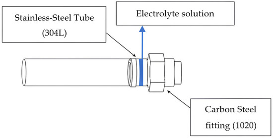
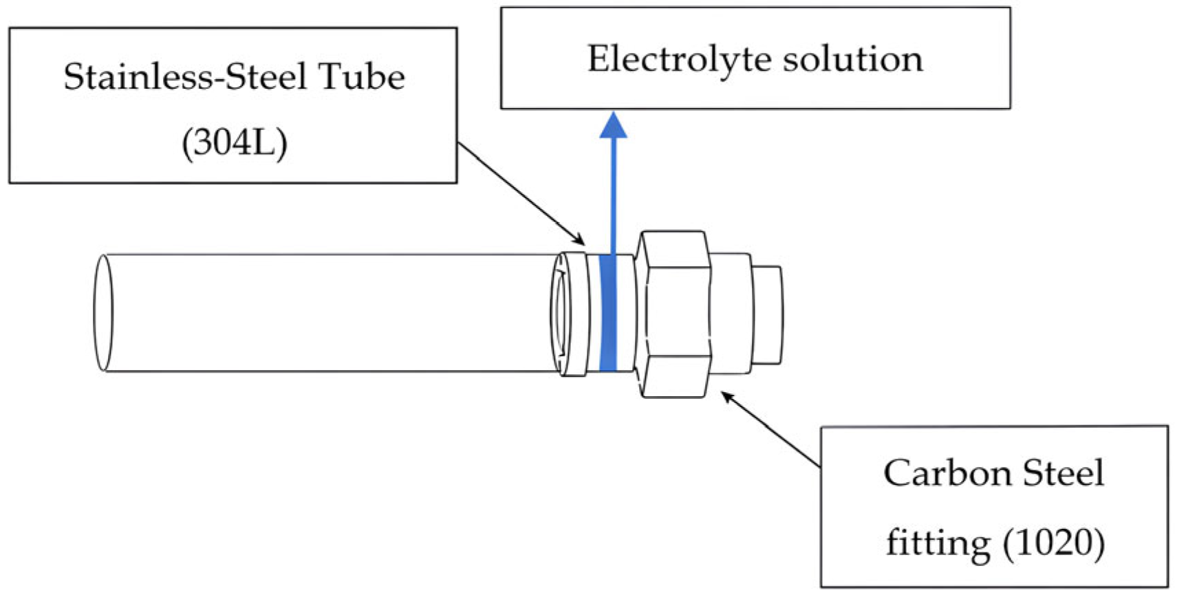
Two different electrolyte concentrations were examined in order to analyze their influence on electrolyte potential and corrosion rate in a galvanic couple [16]. To this end, three galvanic corrosion simulations were carried out for different durations (5, 10, 15 days) in electrolytic environments with two different electrolyte concentrations. Galvanic corrosion therefore took place at the interface between these two materials in the presence of the electrolytic solution (Figure 1). Specifically, 1020 steel acted as an anode, undergoing oxidation, while 304L stainless steel acted as a cathode. The three durations of exposure chosen for this study (5, 10, and 15 days) correspond to both early-stage and intermediate-stage galvanic corrosion, as documented in experimental investigations of steel-couple alloys exposed to sulfide-action environments. These three exposure times have been established as the maximum amount necessary to observe the transition from active-rate to passive-rate partial and complete passivation. Dong et al. also documented this transition in their paper [17]. Longer-term exposures (≥30 days) were not included in this study since the focus of this work is on creating a model that allows the research team to only look at the initial and mid-term stages of corrosion, and did not include any additional effects resulting from corrosion product growth or mass transfer effects, which will be prominent when looking at longer exposures.

Figure 1. Assembly of 304 L steel tube and 1020 steel fitting in contact with electrolytic solution.

Figure 1 provides a schematic representation of a typical industrial assembly, whereas the other figures correspond to the simplified numerical geometry used in the simulations. To model this process, equal anodic and cathodic surface areas were assumed so that the influence of the surface ratio could be ignored and only the effect of the composition of the electrolyte on the evolution over time could be analyzed.

2.2. Geometry and Modeling

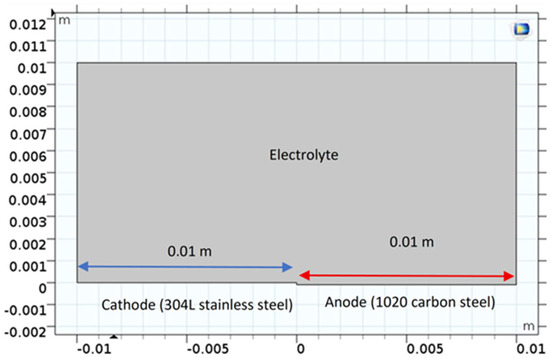
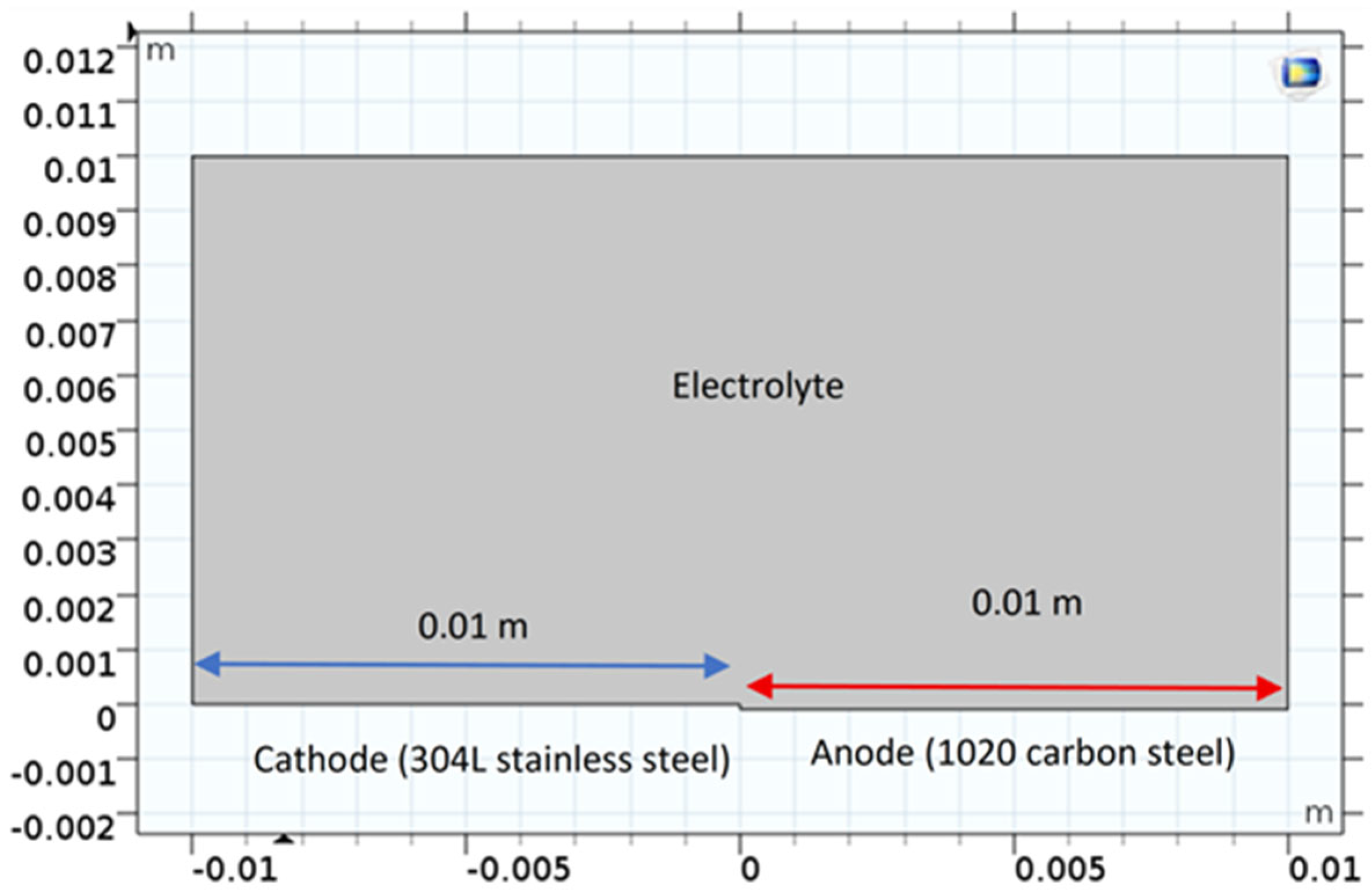
A two-dimensional approach was adopted to simplify the modeling of the contact zone between the two metals in the electrolyte. The geometry includes a flat anode–cathode surface, which represents the contact interface between the two steels. The dimensions of the anode and cathode were chosen to ensure an even distribution of the electric current over the surface. The numerical model was implemented using a two-dimensional geometry with equal anodic and cathodic surface areas (1:1 ratio) in order to isolate the effect of electrolyte composition on galvanic behavior. Therefore, for all the numerical simulations, steady-state conditions were simulated for each immersion period, with constant electrolyte conductivity and activation-controlled kinetics. Figure 2 illustrates the geometry of the model.

Figure 2. Geometric characteristics of the modeling area.

2.3. Study Parameters

The input electrochemical parameters for this simulation were extracted from the experimental potentiodynamic polarization data reported by Dong et al. [17] for both 304L stainless steel and 1020 carbon steel in chloride-containing solutions and then adjusted for numerical convergence requirements in COMSOL. For the 304L stainless steel and 1020 carbon steel, the calculated equilibrium potential and corrosion current densities were obtained from the results of the potentiodynamic polarization measurements performed by Dong et al. [17] in chloride solutions containing sulfides. These values formed the standard input data for the numerical model, although some minor adjustments (in the same order of magnitude) were needed to converge the finite element model.

The corrosion potential for 304L stainless steel was taken directly from the experimental results reported by Dong et al. [17] (≈−530 mV vs. SCE at 0.01 M S²⁻), along with that for 1020 carbon steel (≈−696 mV vs. SCE at 0.01 M S²⁻). Likewise, the experimental corrosion current densities of 0.67 μA·cm⁻² for stainless steel and 1.48 μA·cm⁻² for carbon steel were used in this model. These experimentally validated parameters ensure that the model reflects real-world conditions and any necessary computational adjustments were made.

The following simplifying assumptions were adopted:

(i)

The stainless steel cathode was taken as rigid.

(ii)

The electrochemical reactions were assumed to be activation-controlled and to follow Tafel kinetics [18,19].

(iii)

The electrolyte conductivity was assumed to be constant and homogeneous, which is a common approximation in short-term numerical modeling of galvanic corrosion where concentration gradients in the electrolyte are neglected [18].

(iv)

The mass transport effects were not explicitly modeled since the investigation was primarily focused on the effect of sulfide concentration on galvanic potential distribution. Such assumptions are consistent with previously published FEM corrosion studies.

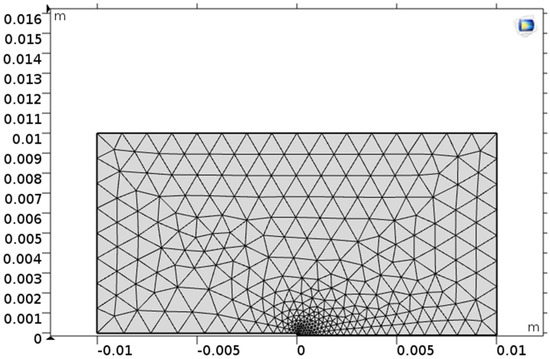
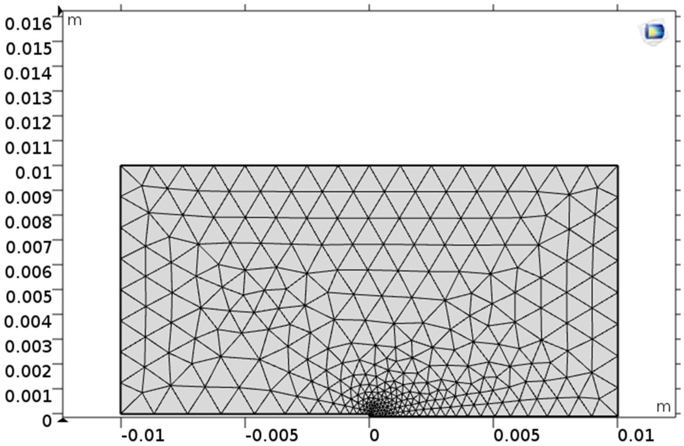
The computational geometry was discretized with a triangular mesh, which was refined at the steel interface to capture localized current density gradients (see Figure 3)

Figure 3. Triangular mesh refined at the steel interface.

The analysis of galvanic corrosion was parametric, taking into account the effect of the materials in contact, the electrolyte concentration, and the exposure time on the electrochemical behavior of the system.

In this study, two types of steel were coupled: a 1020 carbon steel tube (acting as the anode) and a 304L stainless steel fitting (acting as the cathode). The system was immersed in two electrolyte solutions containing chloride and sulfide ions with the following concentrations:

• 0.1 M Cl⁻ + 0.01 M S²⁻;
• 0.1 M Cl⁻ + 0.05 M S²⁻.

For each concentration, tests were conducted over three immersion periods: 5 days, 10 days, and 15 days.

The evolution of the electrolyte potential and the corrosion rate of the 1020 carbon steel under galvanic coupling with 304L stainless steel was evaluated as a function of sulfide concentration and exposure time. The chemical composition of the materials used, namely the 304L stainless steel and 1020 carbon steel, is presented in Table 1 [16].

Table 1. Chemical composition of materials (wt.%).

	C (wt.%)	Cr (wt.%)	Mo (wt.%)	Ni (wt.%)	Mn (wt.%)	Si (wt.%)	P (wt.%)	S (wt.%)	N (wt.%)	Fe (wt.%)
304L	≤0.03	18.0–20.0	≤0.75	8.0–12.0	2.00 max	0.75 max	0.045	0.030	≤0.10	Balance
1020	0.18–0.23	-	-	-	0.30–0.60	≤0.05	≤0.04	≤0.05	-	Balance

The pH and temperature of the electrolyte were assumed to be constant during the simulations and were taken to be identical to the experimental conditions reported by Dong et al. [17] (room temperature and near-neutral pH). Variations in pH and temperature were not explicitly modeled and constitute a limitation of the present approach.

The main parameters defining the galvanic coupling conditions are listed in Table 2. The simulations were carried out using COMSOL Multiphysics^® version 5.1 (COMSOL AB, Stockholm, Sweden), a commercial finite-element software package, using the Electrochemistry Module under an academic license. The governing equations include the law of conservation of charge and Laplace’s equation for the electrolytic potential distribution.

Table 2. Study parameters for the galvanic connection.

Stainless Steel Pipe	Carbon Steel Fitting	Electrolyte Concentration	Time
Fe–18Cr–8Ni		0.1 M Cl− + 0.01 M S2−	5 Days
	Fe–0.20C–0.45Mn		10 Days
		0.1 M Cl− + 0.05 M S2−	15 Days

The deposition of corrosion products on the carbon steel 1020 surface was not considered in the present model since this investigation focused on the early electrochemical stages of galvanic corrosion. This simplification was based on experimental observations reported in the literature for short exposure durations, particularly the work of Dong et al. [17], rather than on direct experimental validation performed in the present study. This simplification has been validated for short-term simulation periods where corrosion product accumulation remains negligible.

The electrochemical parameters used in the simulations are listed in Table 3. The parameters were slightly adjusted to ensure numerical stability. The initial values of these parameters were obtained from the literature to ensure the physical relevance of the model [17]. These adjustments helped prevent certain errors that are often encountered during software computation.

Table 3. Simulation parameters for ions concentrations of 0.1 M Cl⁻ + 0.01 M S²⁻ and 0.1 M Cl⁻ + 0.05 M S²⁻.

	0.1 M Cl− + 0.01 M S2−	0.1 M Cl− + 0.05 M S2−
Equilibrium potential (cathode)	−0.35 V	−0.4 V
Exchange current density (cathode)	6.7 × 10−7 A cm−2	6.4 × 10−7 A cm−2
Equilibrium potential (anode)	−0.696 V	−0.877 V
Exchange current density (anode)	1.48 × 10−6 A cm−2	1.45 × 10−6 A cm−2
Electrolyte conductivity	1.44 S m−1	2.16 S m−1
Tafel slopes	Tafel slope (anode): 0.104 V Tafel slope (cathode): 0.12 V	Tafel slope (anode): 0.098 V Tafel slope (cathode): 0.123 V

2.4. Boundary Conditions

This section describes the boundary conditions and the electrochemical equations used to simulate the galvanic corrosion process between 304L stainless steel and 1020 carbon steel.

Analysis of the Electrode Potential Distribution

The analysis in this study was based on a numerical simulation of galvanic corrosion between 304L stainless steel and 1020 steel in the presence of a chloride-containing electrolyte (NaCl + Na₂S solution). The galvanic couple consisted of a 304L steel cathode and a 1020 steel anode.

The relationships between the current density and electrode potential in the anodic and cathodic reactions were assumed to follow Tafel polarization behavior with activation control, as originally described by Tafel [18]. Thus, the net cathodic current density per unit length ic (x) on 304L steel at an electrode potential Ex is given by

$${\mathit{i}}_{\mathit{c}}\left(\mathit{x}\right)={-\mathit{i}}_0({\mathbf{O}}_{\mathbf{2}})\times {\mathbf{10}}^{\left({\displaystyle \frac{{\mathit{E}}_{{\_\mathbf{e}\mathbf{q},\mathbf{O}}_{\mathbf{2}}}-{\mathit{E}}_{\mathit{x}}}{{\mathit{\beta }}_{\mathbf{304}\mathit{L}}}}\right)}$$

(1)

where

• $E_{{\_eq,O}_2}$ is the equilibrium potential of the cathodic reaction (O₂ reduction).
• $i_0\left(O_2\right)$ is the free corrosion current for the oxygen reduction reaction.
• β₃₀₄L is the Tafel parameter for the cathodic reaction on 304L steel.
• Eₓ is the potential of the electrode at point x.

Similarly, the net anodic current density $i_a\left(x\right)$ on 1020 steel is given by [20]

$$i_a(x)=i_0(\mathrm{F}\mathrm{e})\times {10}^{\left({\displaystyle \frac{E_x-E_{\mathrm{e}\mathrm{q},\mathrm{F}\mathrm{e}}}{{\beta }_{1020}}}\right)}$$

(2)

where

• ${\mathit{i}}_{\mathit{a}}\left(\mathit{x}\right)$ is the net anodic current density at point x.
• ${\mathit{i}}_0\left(\mathbf{F}\mathbf{e}\right)$ is the exchange current corresponding to the oxidation reaction of iron on 1020 steel.
• ${\mathit{E}}_{\mathbf{e}\mathbf{q},\mathbf{F}\mathbf{e}}$ is the equilibrium potential of the iron oxidation reaction.
• β₁₀₂₀ is the Tafel parameter for the anodic reaction on 1020 steel.

The equation governing the potential distribution in the chloride-containing electrolyte follows Laplace’s equation (assuming constant conductivity) [21,22].

$${\mathsf{\nabla }}^{\mathbf{2}}\mathit{\theta }=\mathbf{0}$$

(3)

The resolution of this equation was carried out using software based on the finite element method (FEM) with the application of appropriate boundary conditions. At the electrode–electrolyte interfaces, both anodic and cathodic processes take place simultaneously, and the resulting current density across the interface is determined by these electrochemical reactions.

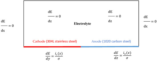
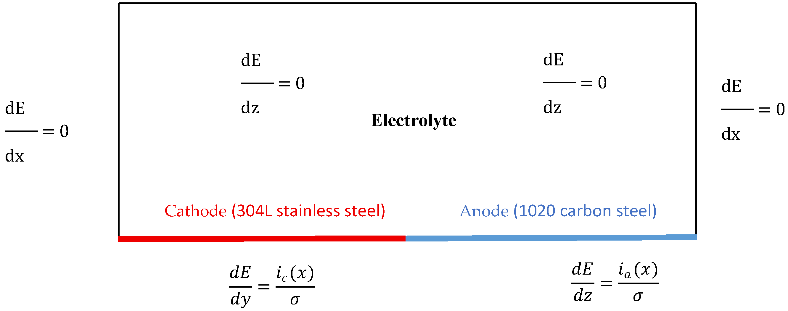
Figure 4 shows the boundary conditions used to solve the electrolyte potential distribution in the galvanic corrosion model. The analysis focused on the impact of different S²⁻ ion concentrations on electrolytic potential distribution and corrosion rate. The results obtained enabled us to quantify the corrosion rate of 1020 steel and explore its evolution in different solutions at different times.

Figure 4. Boundary conditions.

The electrochemical simulations were performed under steady-state conditions for each selected exposure time (5, 10, and 15 days). Each “time” point therefore represents an independent steady-state solution rather than a transient evolution. Mass transport effects and the formation of corrosion-product layers were not explicitly considered in the model. The time-dependent behavior observed in the results was interpreted based on literature reports of FeS film formation and sulfide-induced corrosion mechanisms rather than being directly computed within the numerical framework.

3. Results

To provide a baseline for the interpretation of galvanic corrosion progression, an initial reference state corresponding to an immersion time approaching 0 day (approximately 1 h after immersion) was considered. At this early stage, the galvanic couple is assumed to be free of corrosion products, and the electrolyte potential distribution and current density reach their maximum values due to the absence of any attenuation or passivation effects. This initial state serves as a conceptual reference for interpreting the subsequent evolution of galvanic behavior observed at 5, 10, and 15 days.

3.1. Potential of the Electrolyte

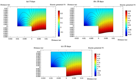
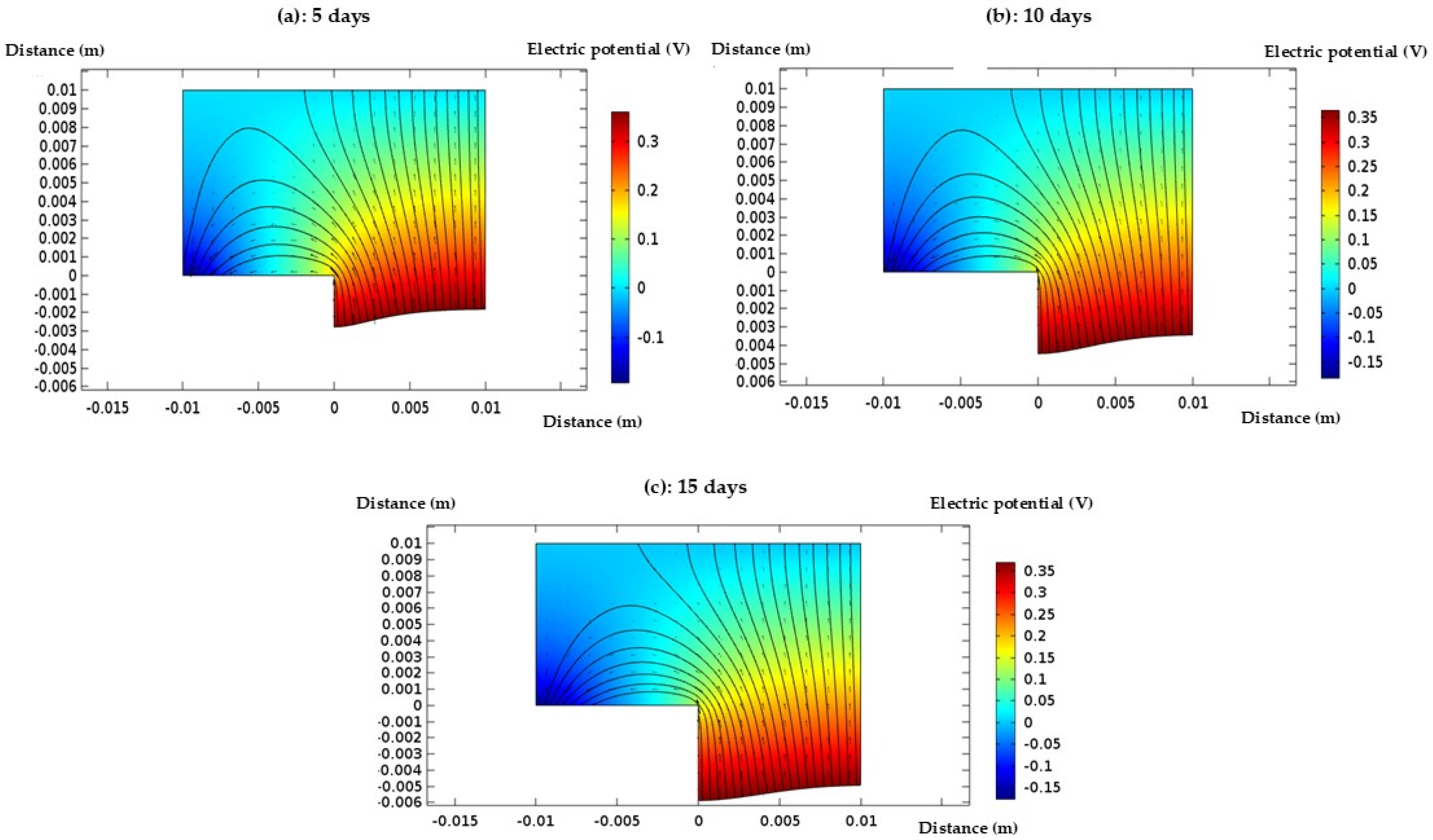
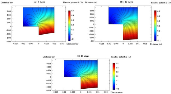
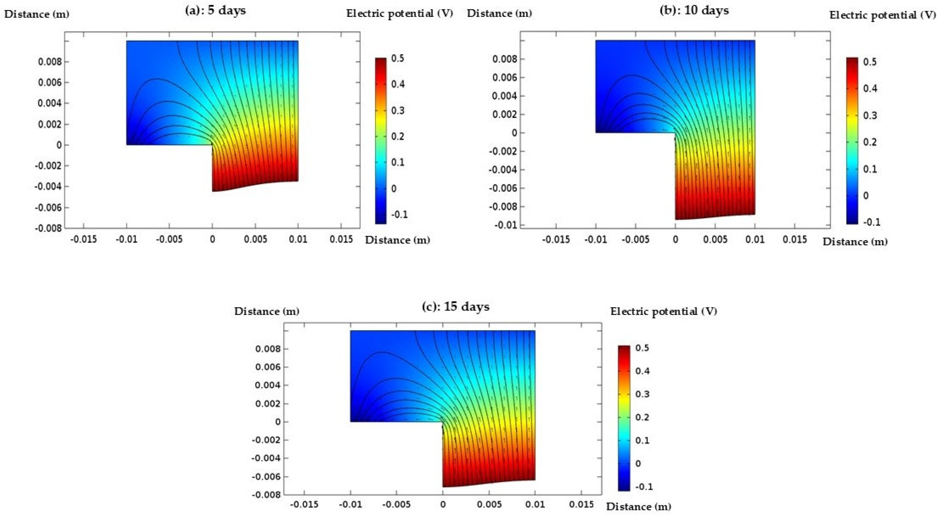
After defining the electrochemical parameters, the model geometry was created, the boundary conditions were applied, and a suitable mesh was generated to ensure accurate numerical resolution. The simulation of galvanic corrosion was then performed. By solving Laplace’s equation, the distribution of the electrolyte potential across the surfaces of the tube and fitting electrodes was obtained. This potential distribution provides insight into the electrochemical behavior at the electrode–electrolyte interface. Figure 5 and Figure 6 illustrated the evolution of the electrolyte potential on the deformed geometry at different time steps for two distinct concentrations of the electrolyte solution, highlighting the influence of concentration on the corrosion process.

Figure 5. Distribution of electric potential (V) in the electrolyte domain after (a) 5 days, (b) 10 days, and (c) 15 days of exposure in Electrolyte 1 (0.1 M Cl⁻ + 0.01 M S²⁻). A progressive reduction in the potential gradient is observed after 15 days, indicating a decrease in the galvanic driving force with exposure time.

Figure 6. Distribution of electric potential (V) in the electrolyte domain after (a) 5 days, (b) 10 days, and (c) 15 days of exposure in Electrolyte 2 (0.1 M Cl⁻ + 0.05 M S²⁻). The current density decreases with increasing exposure time, with the lowest values observed after 15 days, reflecting a reduced galvanic interaction.

The analysis of the electrolyte potential maps at days 5, 10, and 15 reveals a persistent and well-defined gradient between the anodic zone (1020 steel) and the cathodic zone (304L steel), which is characteristic of an active galvanic corrosion process. As early as day 5, the strong concentration of current vectors around the anode indicates intense electrochemical activity, marking the onset of corrosion in the absence of any protective barrier. This behavior continues at day 10, with even more localized current near the anode, confirming that the environment remains aggressive and unfavorable to passivation. At day 10, the environment remains aggressive due to the relatively low sulfide concentration (0.01 M S²⁻), which is insufficient to promote the formation of a continuous or protective corrosion product layer. Under such conditions, chloride-induced anodic dissolution dominates, maintaining high galvanic activity. By day 15, although a slight reduction in current intensity is observed, likely due to the accumulation of corrosion products or local saturation of the electrolyte, the potential gradient remains significant. This confirmed the persistence of galvanic corrosion, with a sustained electrochemical imbalance: the 1020 steel continues to corrode actively, while the 304L steel maintains its cathodic role [22].

Figure 6 presents the potential maps over the 15-day period for the second concentration which illustrate a progressive shift in the galvanic corrosion dynamics due to the higher sulfide concentration. At day 5, the potential gradient between the anodic (1020 steel) and cathodic (304L steel) zones remains visible but is slightly less pronounced than in the 0.01 M S²⁻ case. This attenuation suggests the early onset of a protective mechanism. It should be emphasized that FeS film formation is not explicitly simulated in the present model; instead, the reduced galvanic activity observed numerically is interpreted in light of experimental studies reporting FeS-induced passivation under similar chloride–sulfide conditions.

By day 10, the potential distribution becomes more homogeneous, and the current density around the anode is less concentrated, indicating a noticeable reduction in electrochemical activity. This change pointed to the growing influence of the FeS film, which appears to act as a partial barrier, limiting anodic dissolution and thus slowing the galvanic corrosion process. While corrosion is not entirely suppressed, the formation of the protective layer significantly enhances the system’s resistance.

At day 15, the potential becomes nearly uniform across the electrolyte, and current vectors are much weaker and more diffuse. This configuration reflects a substantial decline in electrochemical activity, signaling that the 1020 steel has reached a passivated state. The well-developed FeS layer now serves as an effective protective film, significantly impeding ion access to the metal surface and drastically reducing corrosion. These observations confirmed the effectiveness of sulfide-induced passivation in mitigating galvanic corrosion under these conditions [23,24].

3.2. Corrosion Rate

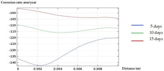
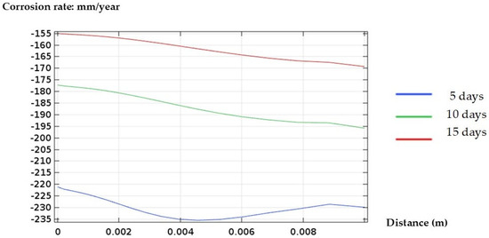
The corrosion rate is a critical parameter for evaluating the severity and progression of material degradation in galvanic systems. In this study, the corrosion rate was monitored over time under different electrolyte concentrations to assess the influence of sulfide ion levels on the corrosion behavior of 1020 steel in contact with 304L stainless steel. Figure 7 and Figure 8 present the corrosion rates in the solutions with two different electrolyte concentrations.

Figure 7. Corrosion rate distribution (mm·year⁻¹) after 5, 10, and 15 days in Electrolyte 1 (0.1 M Cl⁻ + 0.01 M S²⁻). The corrosion rate decreases with increasing exposure time, indicating a progressive reduction in galvanic corrosion activity.

Figure 8. Corrosion rate distribution (mm·year⁻¹) after 5, 10, and 15 days in Electrolyte 2 (0.1 M Cl⁻ + 0.05 M S²⁻). A higher sulfide concentration leads to lower corrosion rates at longer exposure times, reflecting a weakened galvanic interaction.

The evolution of the corrosion rate over the observed period highlights a process of intense and sustained anodic dissolution. By day 5, a high corrosion rate is recorded, indicating an immediate and aggressive attack on 1020 steel [25] starting from the onset of exposure. The results suggest that the environment is particularly harsh, preventing the formation of any protective or passive film on the metal surface and leaving the material highly susceptible to continuous degradation.

At day 10, the continued increase in corrosion rate confirms that the electrolyte remains aggressive, offering no significant resistance to the ongoing electrochemical attack. The absence of protective mechanisms allows the galvanic corrosion to intensify, with 1020 steel, acting as the anode, suffering accelerated deterioration due to its coupling with the more noble 304L steel.

By day 15, although the corrosion rate remains high, a slight tendency toward stabilization is observed. This was attributed to the gradual accumulation of corrosion products on the anode surface, forming a partial barrier [26]. This local saturation could begin to slightly reduce the kinetics of anodic dissolution, without halting the corrosion process altogether, which continues to progress, albeit at a marginally slower rate.

The evolution of the corrosion rate in the solution containing 0.1 M Cl⁻ + 0.05 M S²⁻ reveals a dynamic behavior over the exposure period. During the first 5 days, a high corrosion rate is observed, comparable to that measured in the 0.1 M Cl⁻ + 0.01 M S²⁻ solution at the same time point. This indicates a rapid and intense attack on the metal surface before the formation of a protective layer. By day 10, the corrosion rate begins to decrease, reflecting the emergence of a protective effect. It should be noted that the formation of an iron sulfide (FeS) film was not directly simulated; rather, the numerical decrease in corrosion rate is interpreted based on experimental evidence reported in the literature, which associates higher sulfide concentrations with FeS-induced passivation [27]. This film acts as both a physical and electrochemical barrier, slowing down the corrosion process. By day 15, the corrosion rate drops significantly, well below that observed in the 0.1 M Cl⁻ + 0.01 M S²⁻ solution, indicating the complete and effective formation of a FeS protective layer that enhances the metal’s resistance to corrosion [28].

In comparison, the solution containing 0.1 M Cl⁻ + 0.01 M S²⁻ shows a high and sustained corrosion rate throughout the entire exposure period, without the effective formation of a protective film, resulting in a continuous and aggressive attack on the metal. By day 15, a slight stabilization is observed due to the partial accumulation of corrosion products, but the corrosion rate remains significantly higher than that measured at 0.05 M S²⁻. Thus, a higher sulfide concentration (0.05 M) promotes faster and more effective passivation of the metal [29].

To check the accuracy and reliability of the numerical model developed in the present study, a systematic comparison was conducted with experimental data published by Dong et al. [17] in which the same galvanic couple (1020 carbon steel/304L stainless steel) was investigated in similar chloride and sulfide solutions.

The corrosion potentials, E_corr, and corrosion current densities, i_corr, measured by potentiostatic polarization, are the key electrochemical parameters that were used as direct input data for the COMSOL simulation. They were taken from the work of Dong et al. [17]. For instance, for the 0.01 M S²⁻ solution, values of E_corr = −696 mV/SCE and i_corr = 1.48 μA·cm⁻² for 1020 steel, and E_corr = −530 mV/SCE and i_corr = 0.67 μA·cm⁻² for 304L steel were used. This approach allows the model to be firmly based on the physical and chemical reality of the system.

Comparison of the trends predicted by the model with the experimental results showed remarkable qualitative agreement:

• Influence of Sulfide Concentration: Our modeling gave a correct forecast for the reduction in the corrosion rate of 1020 steel with increasing S²⁻ ion concentration, from an aggressive and sustained attack at 0.01 M S²⁻ to a passivated state at 0.05 M S²⁻. This fully agreed with the findings of Dong et al. [17], who attributed this phenomenon to the formation of a protective iron sulfide (FeS) film at higher sulfide concentrations.
• Galvanic Potential Distribution: The electrolyte potential maps resulting from the simulation here, shown in Figure 5 and Figure 6, indicate a steep potential gradient between the anode and cathode, which is typical for an active galvanic coupling. In fact, this result agrees with the measurement of galvanic potential, E_g, made by Dong et al. [17], which is presented in Figure 2 in their paper and shows that E_g develops with time to reach stable values for different surface ratios.
• Time Evolution: The simulation successfully captured the time evolution of the corrosion process. For example, the steady decrease in current density and potential heterogeneity over 15 days in the 0.05 M S²⁻ solution, as seen in Figure 6, is consistent with FeS layer formation and maturation. This would have a gradual retarding effect on the corrosion kinetics, as suggested by the 15-day mass loss measurements in the referenced experimental study.

Even though this work focused on a simplified geometrical configuration (2D, 1:1 surface ratio) for a basic analysis of the mechanisms, the numerical results obtained are in very good agreement with quantitative experimental data from the literature for the same materials and identical corrosive media. In conclusion, the good agreement between the model-predicted trends and the experimentally observed phenomena validates the adopted modeling approach. These results confirm that the FEM model is capable of reproducing the key mechanisms of galvanic corrosion in mixed Cl⁻/S²⁻ environments, thus making it a reliable predictive tool for further investigations.

4. Discussion

The corrosion behavior of a 304L/1020 galvanic couple arising from this study appears to be very sensitive to changes in sulfide concentration, although all simulations were conducted under identical conditions. The current study is purely numerical and does not involve experimental measurements. Validation of the model was conducted through a comparison with experimental results in the literature for the same galvanic couple and concentrations of the same electrolytes [17]. This practice is common when conducting numerical corrosion research and experimental data are available. A strong difference in the corrosion rate between the two electrolytes proves that small chemical changes in the environment can lead to large variations in anodic dissolution, which was also observed in previous experimental studies. However, it must be emphasized that this mathematical model does not treat or simulate the generation of corrosion products, mass transport, or the generation of protective films. The finite element analysis only simulates the electrochemical reaction of the coupled cell in terms of electrolyte electric potential and current density. Thus, the model does not predict or simulate the passivation mechanisms based on FeS generation but rather relies on experimentally derived data. With a concentration of 0.01 M S²⁻, the sustained potential gradient and high measured rates indicate the absence of an effective protective layer on the 1020 steel, and active corrosion continued. In the other scenario, when the concentration of the sulfide is raised to 0.05 M, the current density is substantially lowered, with a more evenly distributed potential, signifying that the galvanic effect has been diminished. This is in agreement with the formation of the FeS layer and the passivation of the 1020 carbon steel, which has been reported in the literature. Nonetheless, it must be noted that the above COMSOL simulation does not model the transport phenomena or the formation of the corrosion product layer. The effect of the FeS layer is therefore assumed from experimental results rather than being predicted from the simulation. The protective effect of the sulfides has been noted before, but this is not always the case. These results stress the need for a precise definition of local environmental conditions when testing the galvanic corrosion risk. Such a complex problem as the behavior of mixed-metal assemblies exposed to complex electrolytes can hardly be described by a simple indicator like “corrosivity.” Realistic lifetime prediction requires detailed knowledge of ion concentrations and their evolution over time.

Taken altogether, the numerical results presented here contribute to the development of reliable models for mixed chloride–sulfide environments. Dynamic film growth and mass transport effects should be incorporated into future work to further refine the predictive capability of the simulations.

It should be emphasized that the temporal evolution discussed in this work is inferred from literature-reported corrosion mechanisms and not from an explicit simulation of film growth or mass transport.

Although there is good agreement between the calculated and experimental results reported in the literature, the model includes some simplifying assumptions. For example, the geometry was simplified to a two-dimensional system and the electrode surface area was kept fixed. This does not reflect the situation in industrial setups. Additionally, there was no modeling of mass transport processes, electrolyte concentration changes, and corrosion product formation.

These assumptions may influence the quantitative prediction of corrosion rates, particularly at longer exposure times and higher sulfide concentrations. Future improvements to the model could include the incorporation of mass transport effects, dynamic corrosion product layer growth, and three-dimensional geometries with variable anode-to-cathode surface ratios. Experimental validation under controlled laboratory conditions would further enhance the predictive capability of the proposed numerical approach.

To quantitatively verify our results against those from the experimental work performed by Dong et al., the rate of corrosion obtained in this model was compared with experimental values obtained in solutions with similar concentrations of sulfide ions (0.01 M and 0.05 M S²⁻). For both concentrations, since experimental values of the rate of corrosion are not provided, approximate values were obtained through estimates based on experimental plots. In the 0.01 M S²⁻ solution, the experimental rate of corrosion was approximately 26 g·m⁻²·day⁻¹, while in this model, a higher rate of corrosion was observed. However, with a similar increase in sulfide ion concentrations to 0.05 M S²⁻, a significant decrease in both the simulated and experimental rates of corrosion takes place, with a relative decrease of 46% in the simulation and 45% in the experiment.

5. Conclusions

This study numerically investigated the galvanic corrosion behavior of a 304L stainless steel/1020 carbon steel couple in chloride solutions containing different sulfide concentrations using COMSOL Multiphysics. The results demonstrate that sulfide concentration plays a decisive role in controlling galvanic corrosion intensity.

At a low sulfide concentration (0.01 M S²⁻), high electrolyte potential gradients and corrosion rates were maintained over time, indicating sustained anodic dissolution of 1020 carbon steel. However, an increase in the sulfide concentration to 0.05 M S²⁻ resulted in a gradual reduction in the galvanic current density and rates of corrosion, and this was due to the formation of an iron sulfide layer on the surface of the carbon steel.

The numerical results showed good qualitative agreement with experimental data reported in the literature, confirming the ability of the proposed finite element model to reproduce the main mechanisms governing galvanic corrosion in chloride–sulfide environments. Despite the simplifying assumptions adopted, the model provides a reliable framework for understanding galvanic interactions and guiding future experimental and numerical investigations.

References

- Daniel, E.F.; Wang, C.; Li, C.; Dong, J.; Zhang, D.; Zhong, W.; Zhong, S.; Udoh, I.I.; Okafor, P.C. Synergistic effect of crevice corrosion and galvanic coupling on 304 stainless steel fasteners degradation in chloride environments. npj Mater. Degrad. 2023, 7, 11. [Google Scholar] [CrossRef] [Scilit]
- Wu, T.; Qin, J.; Zhang, X.; Qu, S.; Feng, X.; Guo, R. Galvanic corrosion behavior of mill-scaled carbon steel coupled to AISI 304 stainless steel in chloride-contaminated mortar environments. J. Mater. Civ. Eng. 2023, 35, 04023122. [Google Scholar] [CrossRef] [Scilit]
- Frankel, G.S. Pitting corrosion of metals: A review of the critical factors. J. Electrochem. Soc. 1998, 145, 2186–2198. [Google Scholar] [CrossRef] [Scilit]
- Xu, P.; Zhao, M.; Fu, X.; Chen, Z. Effect of chloride ions on the corrosion behavior of carbon steel in an iron bacteria system. RSC Adv. 2022, 12, 15158–15166. [Google Scholar] [CrossRef] [Scilit] [PubMed]
- Zhang, D.; Chen, Y.; Dong, J.; Li, X. Protective role of iron sulfide films formed on steel surfaces in sulfide-containing environments. Electrochim. Acta 2020, 354, 136698. [Google Scholar] [CrossRef] [Scilit]
- Li, D.; Quan, B.; Li, J.; Chen, C.; Xu, J.; Wang, H. Effect of sulfur on synergistic corrosion behavior of Q235 and 16Mn steel in sodium aluminate solution. Sci. Rep. 2024, 14, 22301. [Google Scholar] [CrossRef] [Scilit]
- Imran Ulhaq, M.; Saleem, Q.; Ajwad, H.; Aleisa, R.M.; Alanazi, N.M.; Leoni, M.; Zahrani, I.; Makogon, T. Corrosion Inhibition of Carbon Steel in a Sour (H2S) Environment by an Acryloyl-Based Polymer. ACS Omega 2023, 8, 18047–18057. [Google Scholar] [CrossRef] [Scilit]
- Javidi, M.; Haghshenas, S.M.S.; Shariat, M.H. CO2 corrosion behavior of sensitized 304 and 316 austenitic stainless steels in 3.5 wt.% NaCl solution in the presence of H2S. Corros. Sci. 2020, 163, 108230. [Google Scholar] [CrossRef] [Scilit]
- Parangusan, H.; Bhadra, J.; Al-Thani, N. A review of passivity breakdown on metal surfaces: Influence of chloride- and sulfide-ion concentrations, temperature, and pH. Emergent. Mater. 2021, 4, 1187–1203. [Google Scholar] [CrossRef] [Scilit]
- Liu, K.; Wu, Y.; Liu, H.; Chen, H.; Li, W. Numerical Simulation of Galvanic Corrosion and Electrical Insulation for TC4/304 Galvanic Couple. Materials 2025, 18, 38. [Google Scholar] [CrossRef] [Scilit]
- Yin, L.; Jin, Y.; Leygraf, C.; Pan, J. A FEM model for investigation of micro-galvanic corrosion of Al alloys and effects of deposition of corrosion products. Electrochim. Acta 2016, 192, 110–120. [Google Scholar] [CrossRef] [Scilit]
- Zhu, H.; Leng, M.; Jin, G.; Miao, H. A review of research on galvanic corrosion of aluminum alloys. Fluid Dyn. Mater. Process. 2023, 19, 1907–1923. [Google Scholar] [CrossRef] [Scilit]
- Zhong, X.; Chen, T.; Wang, J.; Huang, S.; Chen, L. A microstructure-sensitive electro-chemo-mechanical phase-field model of pitting and stress corrosion cracking. Corros. Sci. 2024, 232, 112031. [Google Scholar] [CrossRef] [Scilit]
- Harzheim, S.; Hofmann, M.; Wallmersperger, T. Comparison of two mesh-moving techniques for finite element simulations of galvanic corrosion. Acta Mech. 2022, 233, 4427–4439. [Google Scholar] [CrossRef] [Scilit]
- Schneider, J.; Kapfer, K.; Mandel, M.; Mittelbach, A.; Krüger, L. Numerical simulation of corrosion in flanges under consideration of corrosion products and their porosity. Corros. Sci. 2025, 251, 112898. [Google Scholar] [CrossRef] [Scilit]
- Zhang, R.; Cang, Y.; Huang, Y.; Zhang, Q.; Xuan, F.-Z. Experiment and numerical analysis model of the galvanic corrosion of NiCrMoV welded joint under different chloride ion concentrations. Electrochim. Acta 2025, 524, 145970. [Google Scholar] [CrossRef] [Scilit]
- Dong, C.F.; Xiao, K.; Li, X.G.; Cheng, Y.F. Galvanic corrosion of a carbon steel–stainless steel couple in sulfide solutions. J. Mater. Eng. Perform. 2011, 20, 1631–1637. [Google Scholar] [CrossRef] [Scilit]
- Tafel, J. Über die Abhängigkeit des elektrischen Potentials von der Stromstärke bei elektrolytischen Vorgängen. Z. Phys. Chem. 1905, 50, 641–712. [Google Scholar] [CrossRef] [Scilit]
- Bard, A.J.; Faulkner, L.R. Electrochemical Methods: Fundamentals and Applications, 2nd ed.; Wiley: New York, NY, USA, 2001. [Google Scholar]
- Mouloudi, M.; Radouani, R.; Essahli, M.; Chafi, M.; Chhiba, M. Study of corrosion pit propagation in aluminum by numerical simulation using the finite element method. Int. J. Electrochem. Sci. 2021, 16, 21119. [Google Scholar] [CrossRef] [Scilit]
- Radouani, R.; Echcharqy, Y.; Essahli, M. Numerical simulation of galvanic corrosion between carbon steel and low alloy steel in a bolted joint. Int. J. Corros. 2017, 2017, 6174904. [Google Scholar] [CrossRef] [Scilit]
- Oldfield, J.W. Electrochemical theory of galvanic corrosion. In Galvanic Corrosion; Hack, H.P., Ed.; ASTM STP 26188S; ASTM International: West Conshohocken, PA, USA, 1988; pp. 5–22. [Google Scholar] [CrossRef] [Scilit]
- Hack, H.P.; Scully, J.R. Galvanic corrosion prediction using long- and short-term polarization curves. Corrosion 1986, 42, 79–90. [Google Scholar] [CrossRef] [Scilit]
- Mansfeld, F. The relationship between galvanic current and dissolution rates. Corrosion 1973, 29, 403–405. [Google Scholar] [CrossRef] [Scilit]
- Mundra, S.; Provis, J.L. Mechanisms of passivation and chloride-induced corrosion of mild steel in sulfide-containing alkaline solutions. J. Mater. Sci. 2021, 56, 14783–14802. [Google Scholar] [CrossRef] [Scilit]
- Tang, Y.; Li, H.; Zhang, J.; Wang, X.; Liu, Q. Role of Al and Mn in Lightweight Weathering Steel: Influence of Rust Layer Structure on Corrosion Behavior. npj Mater. Degrad. 2024, 8, 32. [Google Scholar] [CrossRef] [Scilit]
- Pessu, F.; Barker, R.; Chang, F.; Chen, T.; Neville, A. Iron sulphide formation and interaction with corrosion inhibitor in H2S-containing environments. J. Petrol. Sci. Eng. 2021, 207, 109152. [Google Scholar] [CrossRef] [Scilit]
- Li, W.; Liu, K.; Wu, J.; Chen, H.; Li, P. Numerical Simulation of Carbon Steel Atmospheric Corrosion under Varying Electrolyte-film Thickness and Corrosion Product Porosity. npj Mater. Degrad. 2023, 7, 3. [Google Scholar] [CrossRef] [Scilit]
- Meng, J.; Li, X.; Guo, F.; Cheng, W.; Jia, R. Influence of Temperature on the Galvanic Corrosion Behavior Between Titanium Alloy and 304 Stainless Steel in a Simulated Marine Environment. Corros. Mater. Degrad. 2025, 6, 50. [Google Scholar] [CrossRef] [Scilit]
Disclaimer/Publisher’s Note: The statements, opinions and data contained in all publications are solely those of the individual author(s) and contributor(s) and not of MDPI and/or the editor(s). MDPI and/or the editor(s) disclaim responsibility for any injury to people or property resulting from any ideas, methods, instructions or products referred to in the content. |
© 2026 by the authors. Licensee MDPI, Basel, Switzerland. This article is an open access article distributed under the terms and conditions of the Creative Commons Attribution (CC BY) license.