


Abstract
Independent Component Analysis (ICA) is a blind source separation technique that has been broadly used in signal and image separation. In order to verify the feasibility of ICA algorithms which will be used for the detection of fabric defect, four kinds of classic ICA algorithms have been chosen and compared in terms of their algorithm performances. The results of simulation experiments show that the separation performances of these algorithms are different and FastICA algorithm has the best separation performance than others.
1. Introduction
In production and manufacture of fabric and garment, quality control usually is a crucial aspect to improve enterprises’ economic benefit and level of management. Inspection of fabric defect is an important process in fabric quality control. Defect inspection, a process of subjective, tedious, and time-consuming work, is usually carried out by human operators. With the development of machine vision and compute technology, Automated Image-based Inspection System (AIIS) offers an attractive alternative to human inspection. In image recognition, finding the shape of object or component is a rather general problem and various solutions are available, depending on the nature of data. Blind Sources Separation (BSS), which does not depend on any prior knowledge of source signals, is the process of estimating unknown source signals from observed signals. Usually BSS take an algorithm of ICA to accomplish source separation. The goal of ICA algorithm is to find a linear representation of non-Gaussian data so that the components are statistically independent.
Currently ICA has an extensive application in communication signal processing, speech signal separation, biomedical signal processing, financial data analysis, array signal processing and general signal analysis ect [1]. As so many domestic and foreign scholars studied ICA algorithms, the application of ICA algorithms in image processing aspect is becoming more and more popular. At present, the applications of ICA algorithms in image processing are mainly focused on image feature extraction [2,3], face recognition and detection [4], image separation, medical im-age processing [5], image watermarking [6], image retrieval, character recognition, remote sensing image processing [7] ect. A few studies have also been reported with the use of ICA for texture analysis. Serzer [8] et al. presented a new method for texture classification, using ICA extracts feature of texture image from non-overlapping window and classifying a subwindows as defective or non-defective based on the Euclidean distance. Tsai Du-Ming [9] et al. proposed a constrained version of the ICA model for detecting defect in low-contrast surface images. In recent years, researchers have proposed various methods on fabric defects, such as Fourier transform, wavelet analysis and neural network [10]. In this paper, we introduced ICA as a computation technique for use in fabric defects detection.
2. ICA Algorithm
2.1. Preprocessing for ICA
To simplify the solution of ICA the observed data should be preprocessed appropriately to make it better meet the basic assumptions of ICA. So before applying an ICA algorithm on the data, it usually undergoes preprocessing [1]. In this section we discuss some preprocessing techniques, such as centering, whitening, that make the problem of ICA estimation simpler and better conditioned. Sometimes PCA may also be used to remove the second-order correlation.
2.1.1. Centering
Centralization is the most basic and necessary preprocessing which is used to center the observed signal. Supposed observation vector set as X and the mean of X is m = E(X), the center can expressed as X’ = X−m, X’→X. After estimating centered data, E(X) = E(X’) = E(X−m) = E(X)−m = 0. From the basic ICA model: X = AS, we can obtain E(X) = E(AS) = AE(S), then E(S) = A−1E(X) = A−1m, where m is the mean that was subtracted in the preprocessing.
2.1.2. Whitening
Another useful preprocessing strategy in ICA is whitening the observed data. Applying a linear transformation to make any multidimensional signal into a whited signal process called whitening, which is also known as sphering. One popular method for whitening is to use the eigenvalue decomposition (EVD) of the covariance matrix E(XXT) = EDET, where E is the orthogonal matrix of eigenvalues of E(XXT) and D is the diagonal matrix of its eigenvectors. The corresponding matrix is called whitening matrix Q = D−1/2ET. We can solve half of the problem by whitening.
2.1.3. PCA
Traditional Principal Component Analysis (PCA) can be used as the preprocessing method of ICA to remove the second order redundancy information. PCA is a kind of orthogonal transformation, but there is still the possibility that the existence of some higher-order redundant information which can influence the data that is transformed.
2.2. Classic ICA Algorithm
2.2.1. Natural Gradient Algorithm
The Natural Gradient algorithm (NG) was first proposed by Amari et al. [11], and the cost function is defined as

where W is de-mixing matrix, E is expectation and pi(yi(t)) is probability density function. The iterative formula of the separation matrix in Eq. (1) is proposed as follows:
where µ is the step factor, Eq. (2) updates the amplitude control separation matrix W in each iteration, it affects the convergence speed and stability. Typically, µ generally use the fixed step size. The nonlinear function of separated signal is
W (t + 1) = W (t) + µ[I − f (y(t))yT (t)]W (t)

Compared with the general gradient , gradient
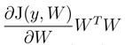 is called natural gradient. Natural gradient algorithm can avoid matrix inverse operation in computational phase, so the algorithm has low computational complexity. Numerical stability is also greatly enhanced while the convergence rate of the algorithm is strengthened to a certain extent.
, gradientis called natural gradient. Natural gradient algorithm can avoid matrix inverse operation in computational phase, so the algorithm has low computational complexity. Numerical stability is also greatly enhanced while the convergence rate of the algorithm is strengthened to a certain extent.2.2.2. Infomax Algorithm
The Infomax algorithm [12] was first put forward by the United States Salk Institute Computational Neuroscience Laboratories researchers. In the basic model, the separated mixture signals y(t) can be expressed as
where B is de-mixing matrix and x(t) is source signal. The model lead into a nonlinear function ri = gi(yi) to replace the estimation of higher order statistics after obtained mixing components y(t) by de-mixing matrix B. The criterion: given appropriate gi(yi), we can find the total entropy weight H(r) of r = [r1, r2, · · · , rM ] maximum. The maximum entropy output form as follows: L = H(G1(y1), G2(y2), · · · , Gn(yn)). where Gi(yi) is a class of nonlinear function.
y(t) = Bx(t)
2.2.3. Extended Infomax Algorithm
An extension of the Infomax algorithm of Bell and Sejnowski based on information theory is able to blindly separate mixed signals with sub-Gaussian and super-Gaussian source distributions. This was achieved by using a simple type of learning rule first derived by Girolami by choosing negative entropy as a projection pursuit index [13]. The algorithm is updated according to the following formula:
where K4 is equal to diag(sign(k4(yi)), k4(yi) is Kurtosis value, sign( ) is sign function, diag( ) put vector into a diagonal matrix.
∆W ∝ [I − K4 tanh(y)yT − yyT ]W

The Fast ICA algorithm [14] based on the principle of non-Gauss maximization, using fixed point iteration theory in order to seek the maximum non Gauss of WT X, which was proposed by Hyvarinen et al. from University of Helsinki in Finland. An algorithm uses Newton’s iterative algorithm to batch process a large number of sampling points of the measured variable X. The approximate Newton iteration formulated as:
where E[ ] is mean operation, g( ) is nonlinear function, g( ) can be interpreted as g1(y) = tanh(a1y), or g2(y) = y exp(−y2/2), or g3(y) = y3 etc. Here, 1 ≤ a1 ≤ 2, we generally take a1=1.
W* = W − [E{Xg(WT X)} − βW ]/[E{g'(WT X)} − β]
3. Simulation
This section is made up of two parts: One is about the separation of mixed signal; the other is about the separation of mixed image. The simulation is completed on a computer whose CPU Type is Intel Corei5 2350M and frequency 2.3 GHz.
3.1. Signal Separation
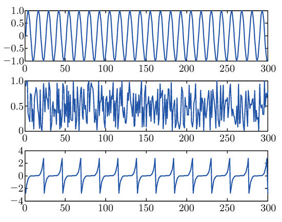
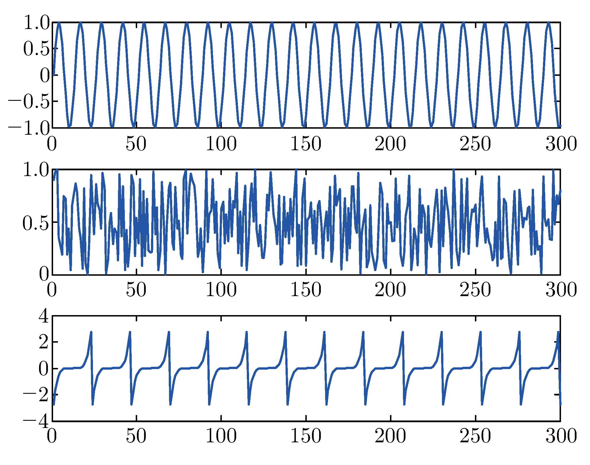
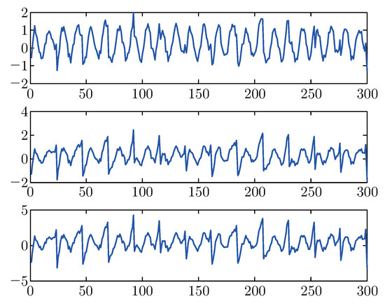
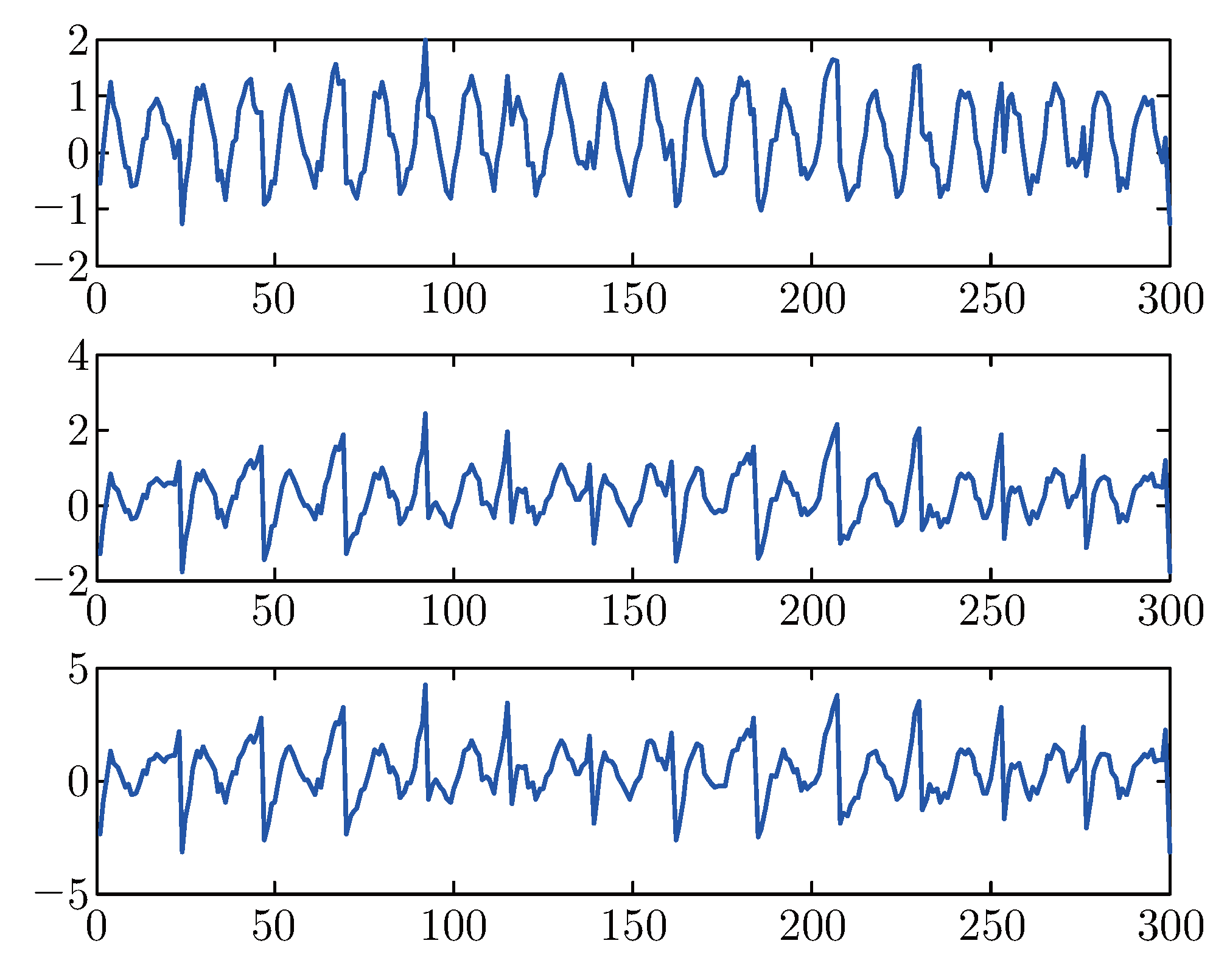
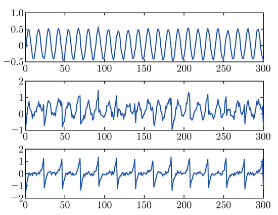
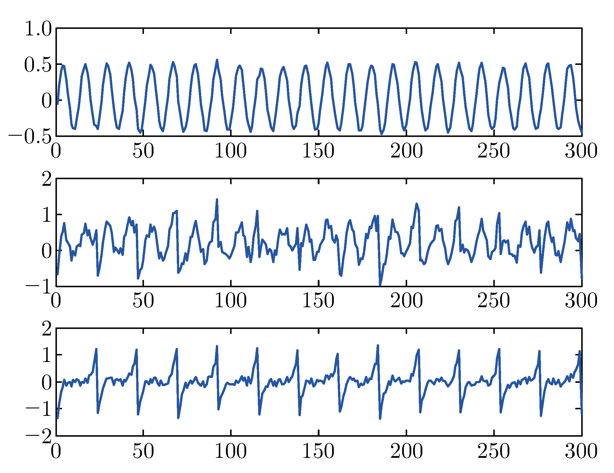
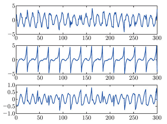
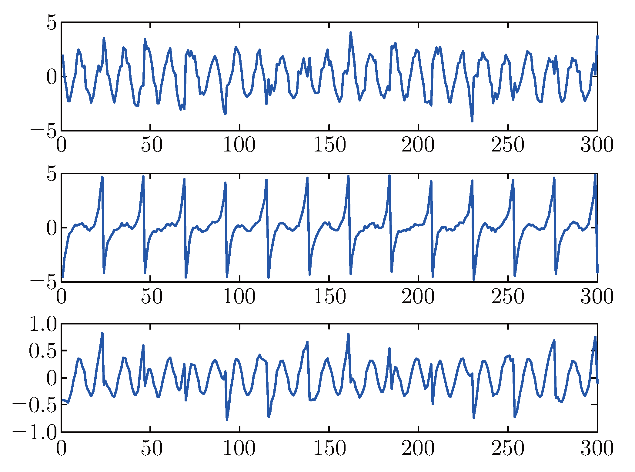
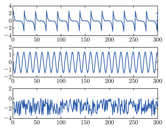
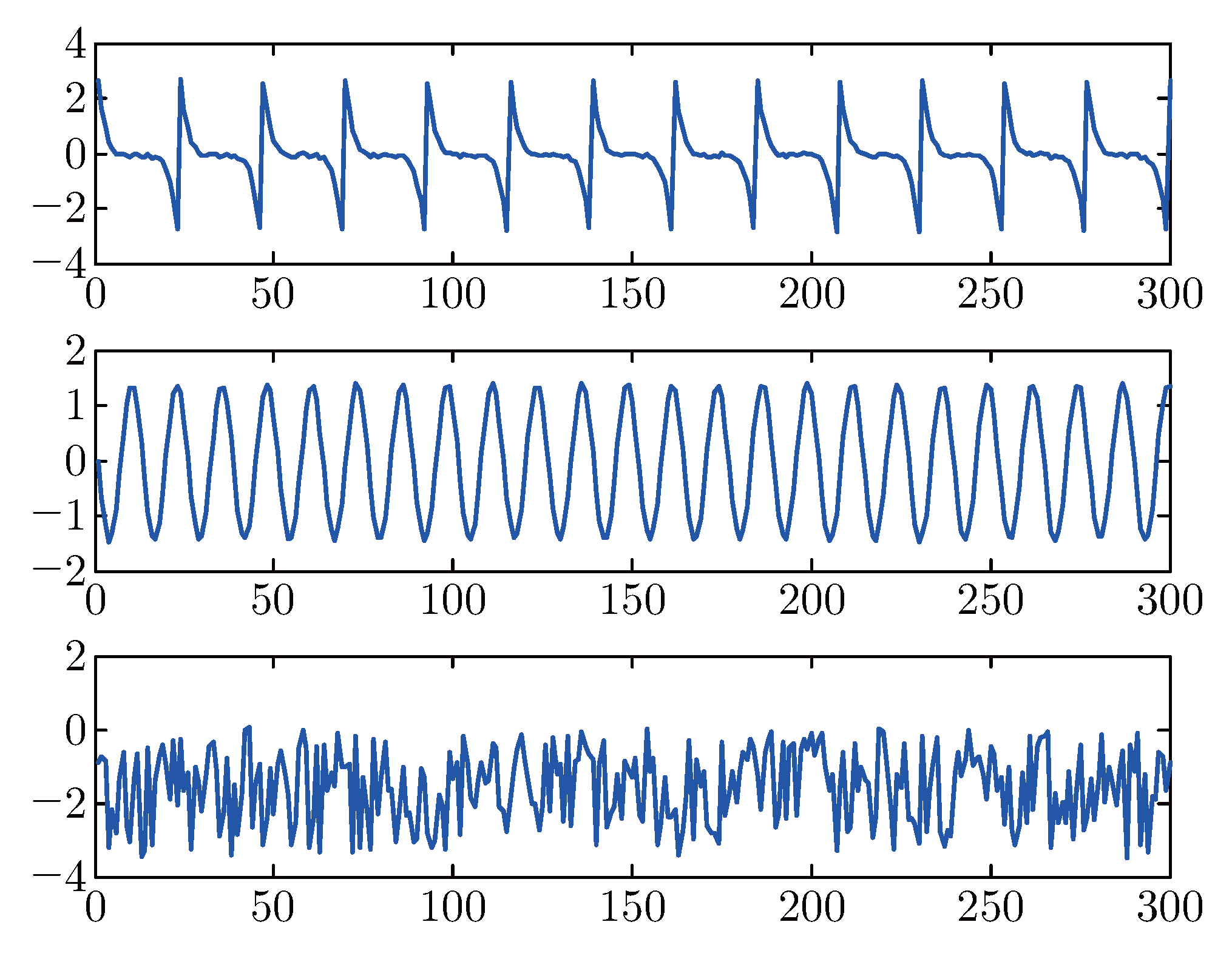
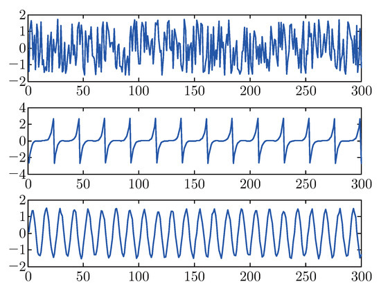
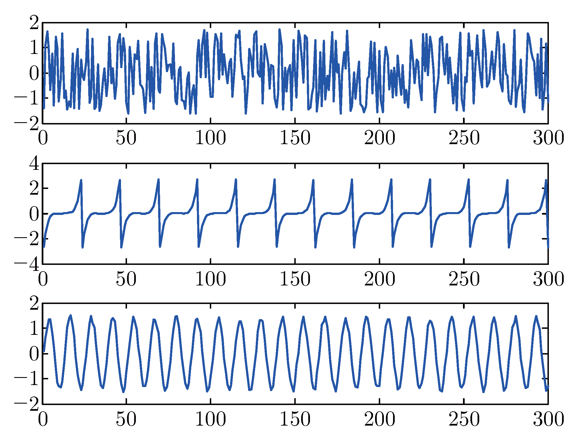
The separation performance of the algorithms mixed in the case of the random mixing matrix was compared by the separation experiment of the mixed sub-Gaussian (s1), Gaussian (s2) and super-Gaussian signal (s3). From top to bottom as shown in Figure 1 the signals are, in order, s1, s2 and s3, which kurtosis value are −0.3738, −0.0096, 2.5145, respectively. In order to effectively compare arithmetic performance, we use the same random mixed matrix W1, which is given by W1=[0.8654 0.5227 0.2278; 0.6126 0.4795 0.4981; 0.9900 0.8013 0.9009]. Figure 2 shows the mixed signals of s1, s2 and s3 with mixed matrix W1. Figure 3, Figure 4, Figure 5, Figure 6 show, respectively, the separated signals y1, y2 and y3 using natural gradient algorithm, Infomax algorithm, extended Infomax algorithm, and FastICA algorithm.
Figure 1.
Source Signals (s1, s2, s3).
Figure 2.
Mixed Signals.
Figure 3.
Separation by NG.
Figure 4.
Separation by Infomax.
Figure 5.
Separation by ExInfomax.
Figure 6.
Separation by FastICA.
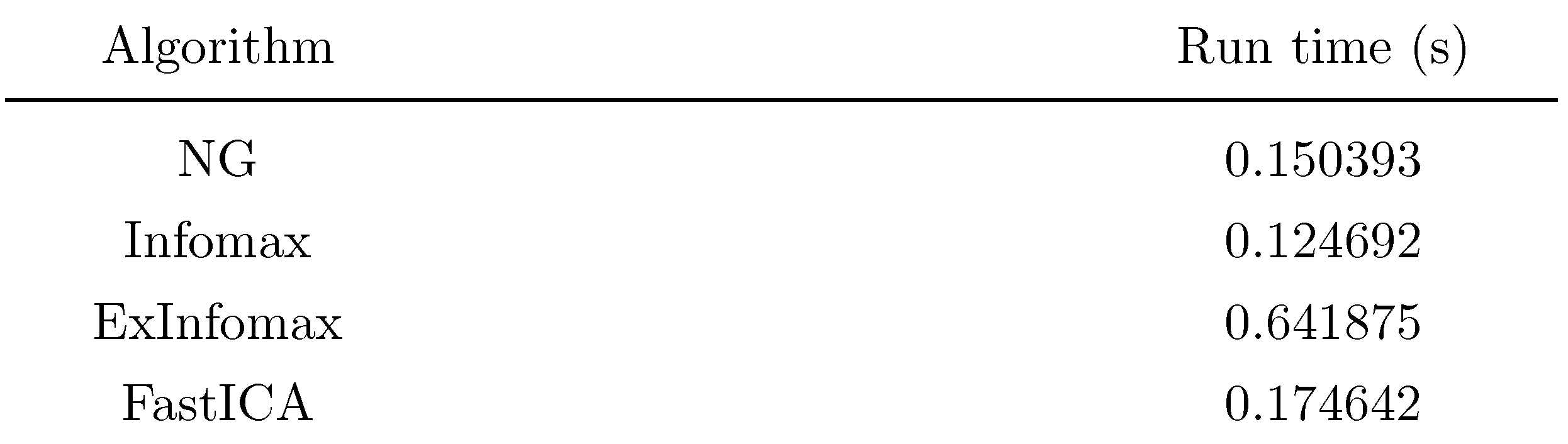
It can be observed from the separation results that the Fast ICA algorithm can well recover the original source signal, whereas the other three algorithms cannot finish it well. Although theseparated sequence and source signals sequence are not consistent, the separated signal waveform of the Fast ICA algorithm is conformed to the originals. Compared with the originals, the wave-forms separated by ExInfomax algorithm have a smaller difference, while waveforms by natural gradient and Infomax algorithm have great difference. The running time of the algorithms is figured out by MATLAB which is given in Table 1 so that we can better compare the algorithms separation performance for mixed signal. The kurtosis value of the signal before and after the separation are also worked out and displayed in Table 2.
Table 1.
The running time of the algorithms.
Table 2.
Kurtosis value of the signal before and after the separation.
As seen in Table 2, the algorithms have different performances to cope with sub-Gaussian (s1), Gaussian (s2) and super-Gaussian signals (s3). It shows NG algorithm have better ability to separate it from the mixed signals while ExInformax and Fast ICA make wrong results and Informax tend to give an unsatisfactory separating results when dealing with the sub-Gaussian signal which kurtosis value equal to −0.3738. Besides, the kurtosis value of s2 before the separation is equal to −0.0096, the result of NG equals 0.0030 is closest. The kurtosis value of s3 before the separation is equal to 2.5145, the result of four algorithm is 0.1599, 1.7253, 2.3099, 2.3614, respectively, after the separation, so we can draw a conclusion that the result of Fast ICA is closest. In general, according to the information shown in Table 1 and Table 2, the Infomax algorithm and natural gradient algorithm work more efficiently than Fast ICA algorithm, but their separation effect are worse than it. Furthermore, the effect of the Infomax algorithm is not ideal when sub-Gaussian signal was separated. Compared with several other algorithms, kurtosis values of the separated signals used Fast ICA algorithm are closer to the originals.
3.2. Image Separation
This section is divided into two parts: the first part is the separation of natural gray images; the second part is the separation of fabric defect images. In order to evaluate the performance of the algorithm, the performance index is used.
Performance index [15] can be calculated using the equation as follow:

where gij is the i-th row and j-th column element of the global matrix G=WA, maxj|gij| represents the maximum value of the i-th row vector of |G|, and maxj|gji| represents the maximum value of the i-th column vector of |G|. The performance index is zero, ideally, the separation performance achieved perfect. In fact, PI values around 10−2 show that the algorithm has a very good performance.
3.2.1. Natural Gray Images
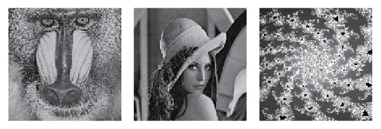
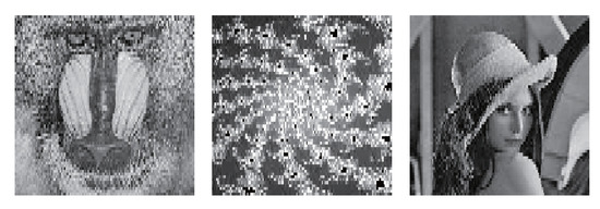
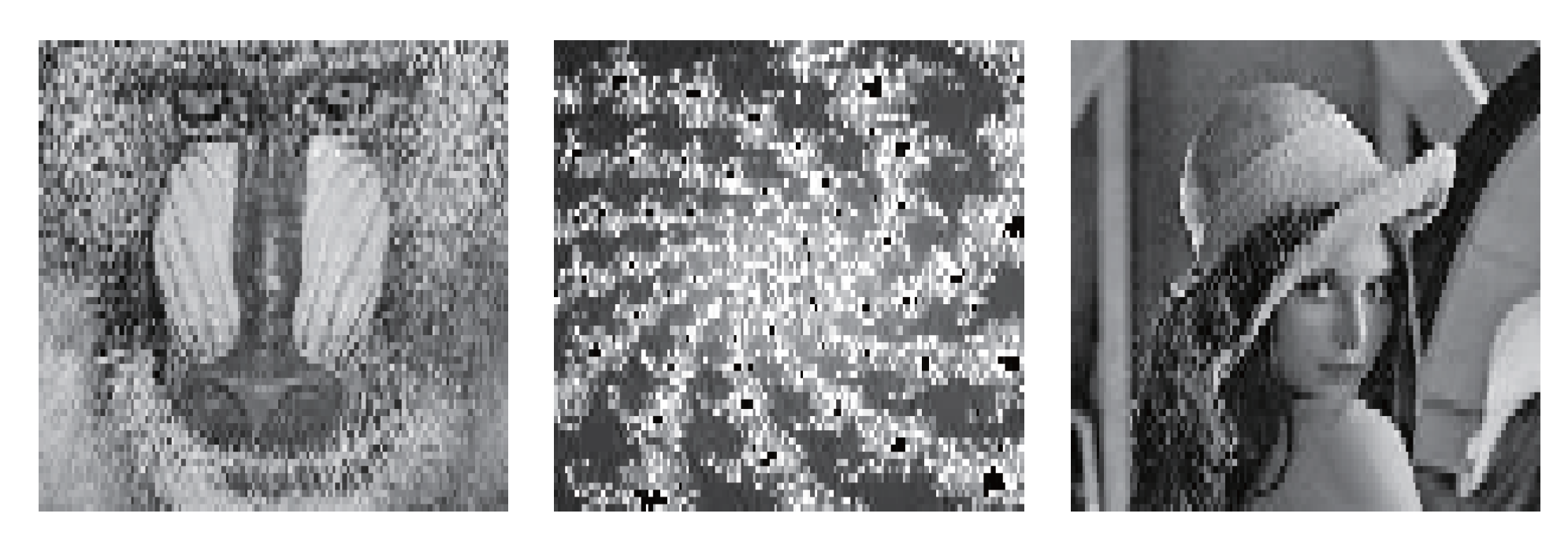
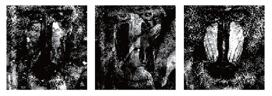
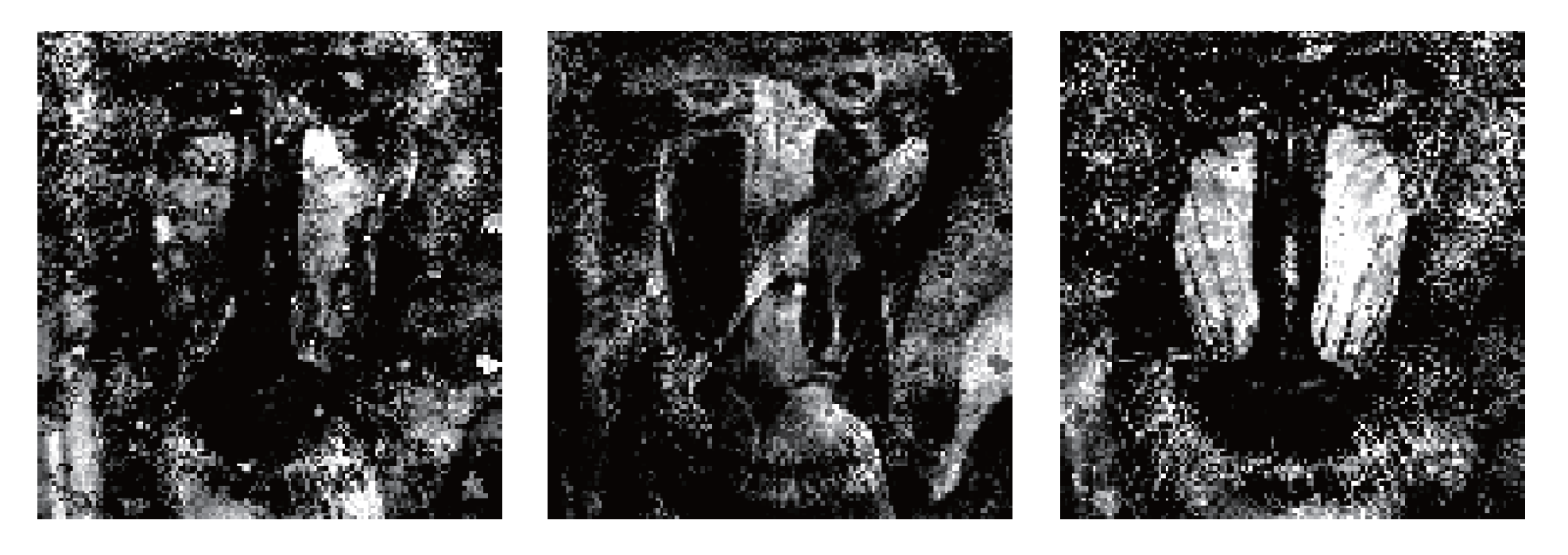
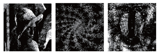
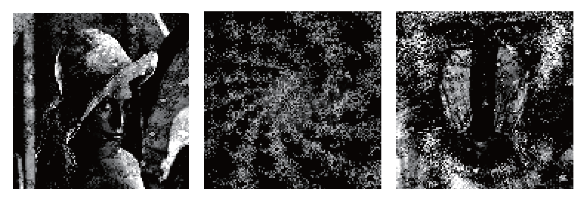
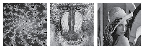
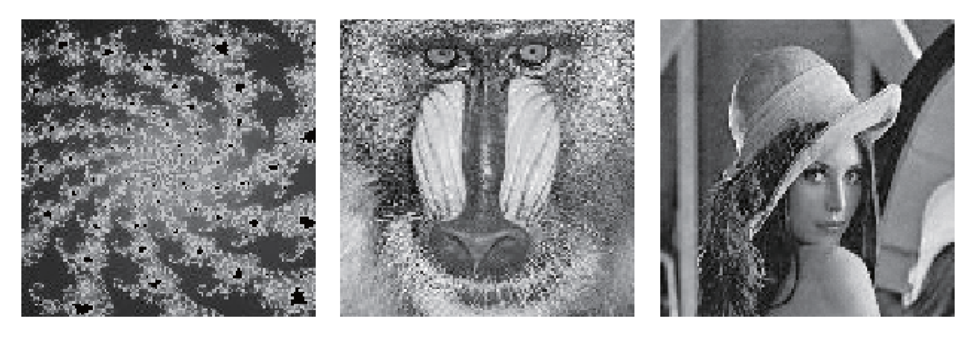
The sizes of test images, from natural image benchmarks, are of 256 pixel × 256 pixel and mixed by random matrix. We used the same random mixing matrix W2 = [0.7922 0.0357 0.6787; 0.9594 0.8491 0.7577; 0.6557 0.934 0.7431] to validly compare the algorithm performance. Figure 7 shows three natural images and Figure 8 mixed images. The separation results are displayed in Figure 9, Figure 10, Figure 11 and Figure 12, respectively. The running time and the performance index are depicted in Table 3.
Figure 7.
Natural images.
Figure 8.
Mixed images.
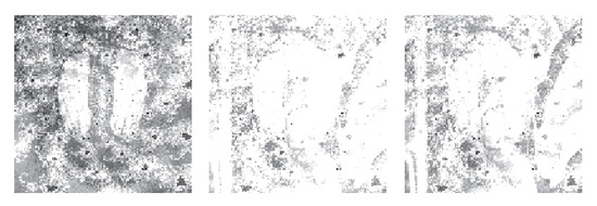
Figure 9.
Separation by NG.
Figure 10.
Separation by Infomax.
Figure 11.
Separation by ExInfomax.
Figure 12.
Separation by FastICA.
Table 3.
The separation performance index and the running time.
From those images, it can be observed that the separated images using natural gradient algo-rithm, extended Infomax algorithm, and FastICA algorithm respectively are consistent with the source image; however, the separation of Infomax algorithm is not well done as shown in Figure 10.
The data in Table 3 shows that running time for separating the natural mixed images with Fast ICA algorithm requires 0.38 s, compared with 4.41 s with ExInfomax algorithm. As is clearly shown above, PI value of Fast ICA algorithm is smaller than Infomax and ExInfomax algorithm. So Fast ICA algorithm separation is excellent. In spite of the best separation effect of natural gradient algorithm for natural image, the calculation time is longer than Fast ICA.
3.2.2. Fabric Defect Images
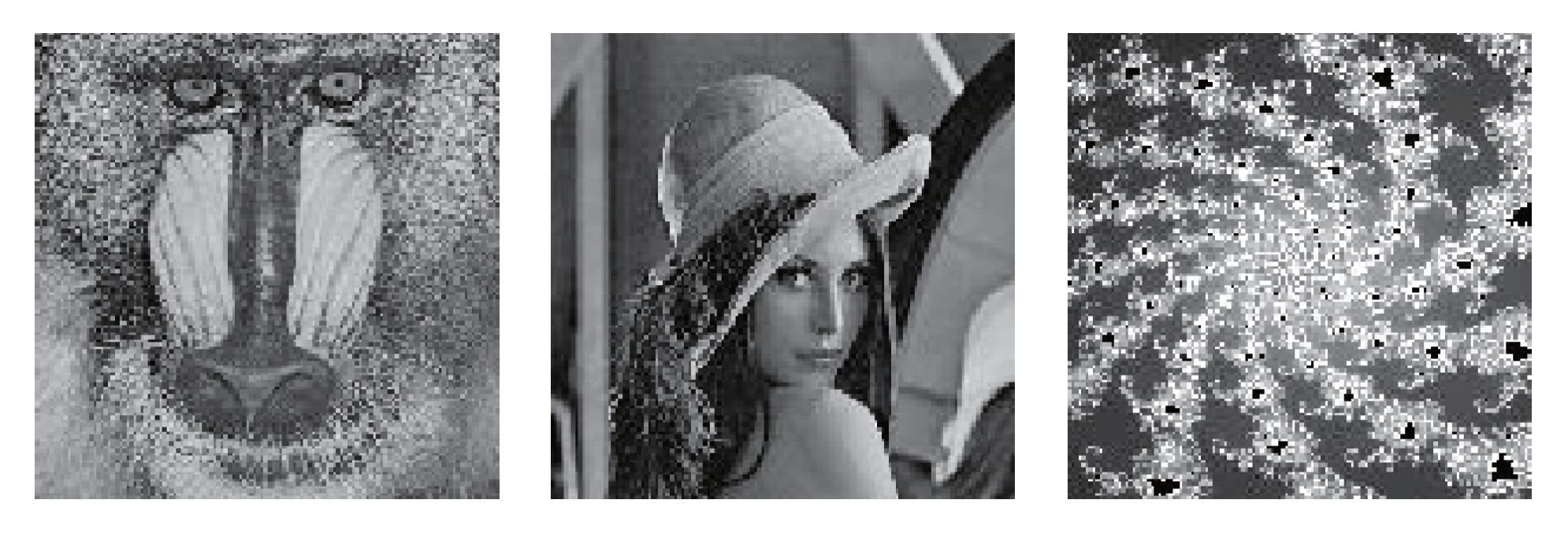
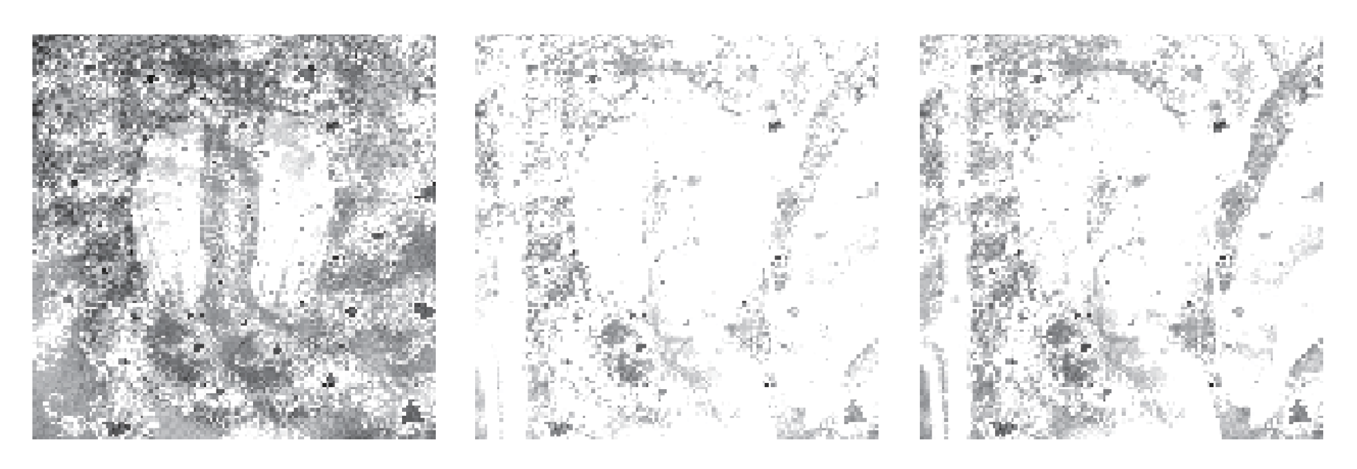
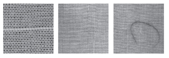
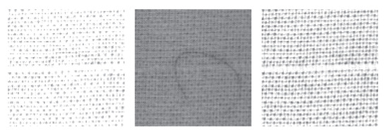
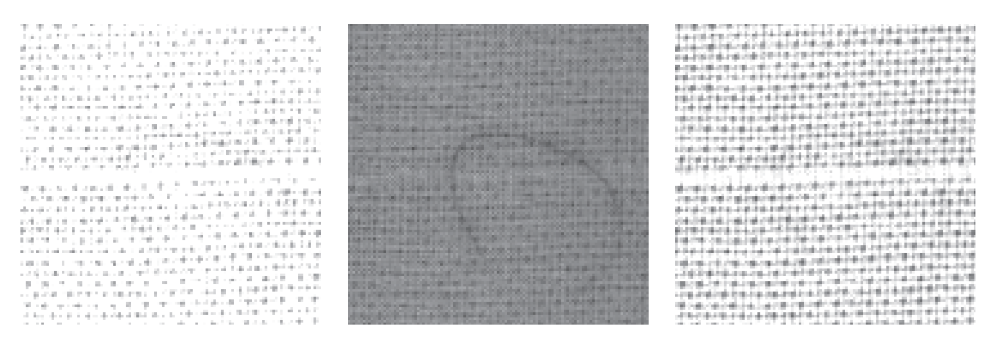
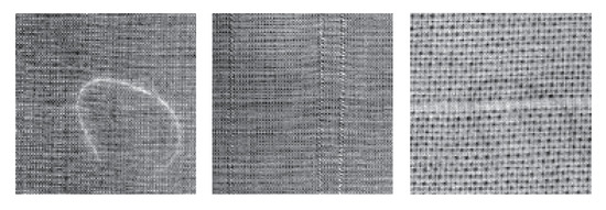
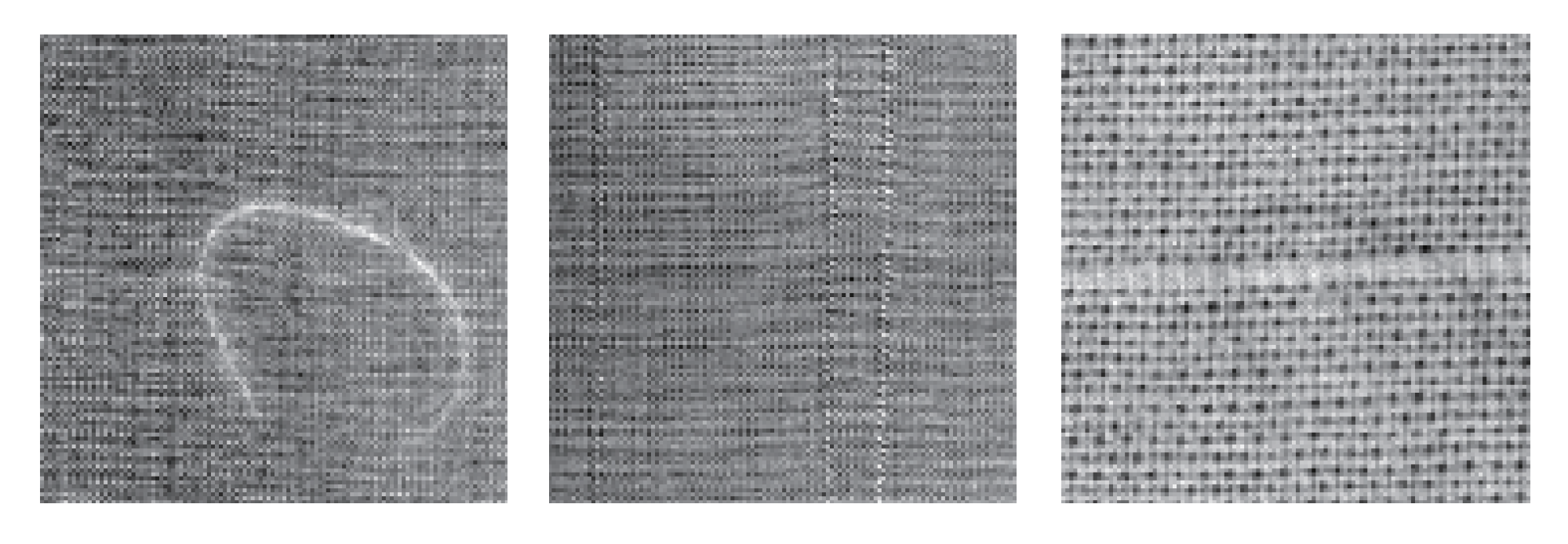
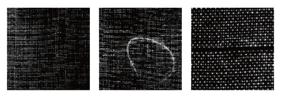
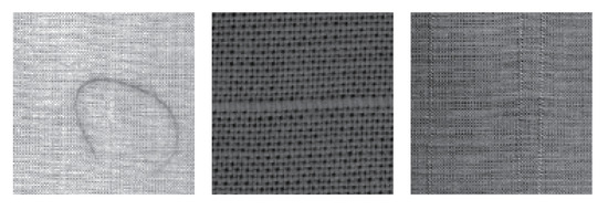
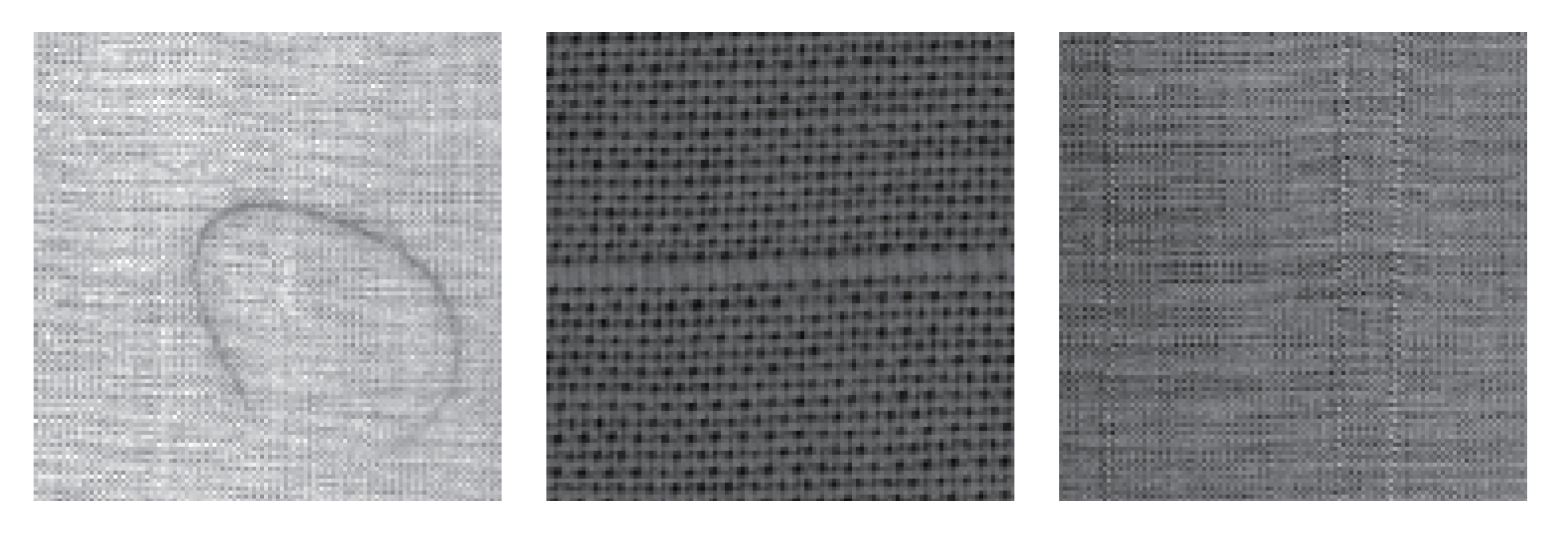
Three fabric defect images, i.e., coarse pick, cracked end, gout, are selected, which size is all the same as 256×256 and mixed by random matrix. The same random mixing matrix W3=[0.8143 0.3500 0.6160; 0.2435 0.1966 0.4733; 0.9293 0.2511 0.3517] are employed. The original Fabric defect images are shown in Figure 13 and mixed images a in Figure 14. Separated by the algorithm of NG, Infomax, ExInfomax and FastICA, the results are given in Figure 15, Figure 16, Figure 17 and Figure 18. The running time of the algorithms as well as the performance index are presented in Table 4.
Figure 13.
Fabric defect images.
Figure 14.
Mixed images.
Figure 15.
Separation by NG.
Figure 16.
Separation by Infomax.
Figure 17.
Separation by ExInfomax.
Figure 18.
Separation by FastICA.
Table 4.
The separation performance index and the running time.
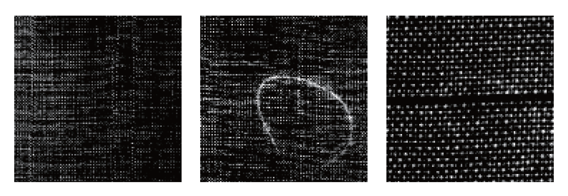
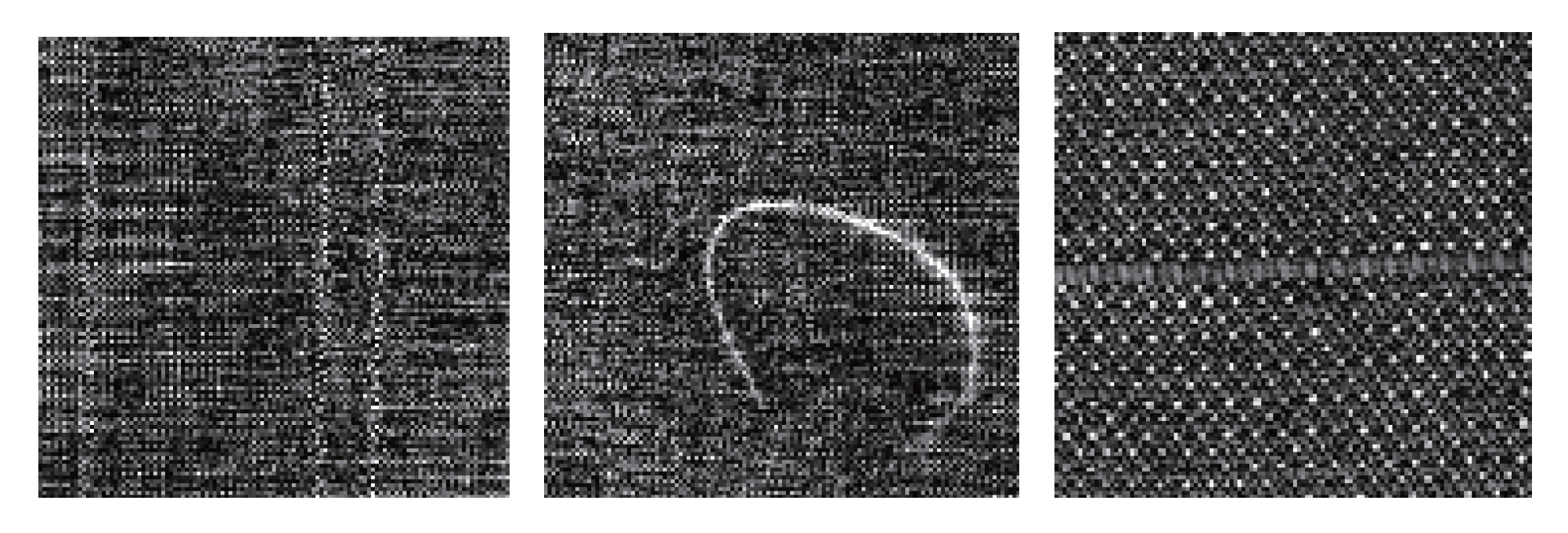
It can be observed from the experimental results that the Fast ICA algorithm and NG can well recover the original image, whereas the other two algorithms cannot finish it well. Although the separated sequence and source signals sequence are not consistent, the separation image of the Fast ICA and NG are conformed to the originals.
From Table 4, we observed the Fast ICA provides better execution time compared to Infomax, NG and ExInfomax. PI value of the Fast ICA algorithm shows that Fast ICA’s separation is alsoexcellent. The image separation simulation test results of Section 3.2.1 and Section 3.2.2 can be concluded that the Fast ICA algorithm outperforms ExInfomax algorithm, Infomax and natural gradient in terms of image separation.
4. Conclusion
This paper makes a comparative research using four ICA algorithms on signal separation and image separation performance. Experimental results show that the separation performances of four algorithms are different. In order to effectively compare arithmetic performance, we used the same random mixed matrix, respectively. In the aspect of signal separation, Fast ICA can well separate the three mixed signal, while Infomax algorithm for sub-Gaussian signal separation is not ideal. In terms of image separation, Fast ICA separation performance is still the best, and Infomax algorithm can separate the fabric defect image, whereas the natural image cannot be separated completely. Although this paper only introduced the ICA in signal processing and image processing application, the application of ICA is utilized widely. The experiment was conducted to evaluate the performance of those algorithms. At present, there are many ways for defect detection. Compared to other detection method, ICA is a method based on the high order statistics and this method for fabric defects detection is worth further study. Using ICA with other intelligent optimization algorithms for fabric defection is the next thing we need to do and further research is underway. With the constant improvement of ICA theory and further promotion, the ICA technology will surely make more contribution to the fabric defects detection in the future.
Acknowledgments
This work was financially supported by the Priority Academic Program Development of Jiangsu Higher Education Institutions.
References
- Hyv¨arinen, A.; Oja, E. Independent component analysis: algorithms and applications. J. Neural Netw. 2000, 13, 411–430. [Google Scholar] [CrossRef] [Scilit]
- Kwak, N.; Choi, C.H. Feature extraction based on ICA for binary classification problems. IEEE Trans. Knowl. Data Eng. 2003, 15, 1374–1388. [Google Scholar] [CrossRef]
- Talbar, S.N.; Bodade, R.M. Feature Extraction of Iris Images using ICA for Person Authentication. ICSPC 2007, 1055–1058. [Google Scholar] [CrossRef] [Scilit]
- Draper, B.A.; Baek, K.; Bartlett, M. S.; et al. Recognizing faces with PCA and ICA. J. Comput. Vis. Image Understand 2003, 91, 115–137. [Google Scholar] [CrossRef] [Scilit]
- Arakeri, M.P.; Reddy, G.R.M. A comparative performance evaluation of independent component anal-ysis in medical image de-noising. ICRTIT 2011, 770–774. [Google Scholar] [CrossRef] [Scilit]
- Gonzalez-Serrano, F.J.; Molina-Bulla, H.Y.; Murillo-Fuentes, J.J. Independent component analysis ap-plied to digital image watermarking. ICASSP 2001, 3, 1997–2000. [Google Scholar] [CrossRef] [Scilit]
- Chiang, S.S.; Chang, C.I.; Ginsberg, I.W. Unsupervised hyper spectral image analysis using independent component analysis. IGARSS 2000, 7, 3136–3138. [Google Scholar]
- Sezer, O.G.; Ertiizun, A. Independent component analysis for texture defect detection. J. Pattern Recognit. 2004, 14, 303–307. [Google Scholar]
- Tsai, D.M.; Lin, P.C.; Lu, C.J. An independent component analysis-based filter design for defect de-tection in low-contrast surface images. J. Pattern Recognit. 2006, 39, 1679–1694. [Google Scholar] [CrossRef] [Scilit]
- Mahajan, P.M.; Kolhe, S.R.; Patil, P.M. A review of automatic fabric defect detection techniques. Adv. Comp. Res. 2009, 1, 18–29. [Google Scholar]
- Amari, S.I. Natural gradient works efficiently in learning. J. Neural Comput 1998, 10, 251–276. [Google Scholar] [CrossRef] [Scilit]
- Bell, A.J.; Sejnowski, T.J. An information-maximization approach to blind separation and blind deconvolution. J. Neural Comput 1995, 7, 1129–1159. [Google Scholar] [CrossRef] [Scilit]
- Lee, T.W.; Girolami, M.; Sejnowski, T.J. Independent component analysis using an extended infomax algorithm for mixed sub-gaussian and super-gaussian sources. J. Neural Comput 1999, 11, 417–441. [Google Scholar] [CrossRef] [Scilit]
- Hyvarinen, A. Fast and robust fixed-point algorithms for independent component analysis. J. Neural Netw. 1999, 10, 626–634. [Google Scholar] [CrossRef] [Scilit]
- Mansour, A.; Kawamoto, M.; Ohnishi, N. A survey of the performance indexes of ICA algorithms. J. MIC 2002, 660–666. [Google Scholar]

© 2014 Textile Bioengineering and Informatics Society. This article is an open access article distributed under the terms and conditions of the Creative Commons Attribution (CC BY) license (https://creativecommons.org/licenses/by/4.0/).