New Statistical Approach to Forecasting Earth’s Skin Temperature from MERRA-2 Satellite Using Semiparametric Time Series Regression with Mixed Additive Spline Fourier (STSR-MASF)

Highlights

What are the main findings?

• The first contribution of this study is the introduction of a new Semiparametric Time Series Regression approach, supported by the theoretical formulation of the STSR-MASF estimator through Lemma and Theorem, along with the construction of the GCV criterion for optimal knot and oscillation selection.
• The second contribution is that an analysis of Earth’s skin temperature in East Kalimantan showed clear warming tendencies and seasonal dynamics, which are captured more accurately by STSR-MASF. This demonstrates the model’s practical usefulness for understanding environmental patterns and informing climate-related decisions in tropical ecosystems.

What are the implications of the main findings?

• The STSR-MASF consistently shows better performance than the six previous methods forecasting methods across all training and testing schemes, producing highly accurate predictions and effectively capturing complex time series patterns.
• The STSR–MASF provides a flexible and reliable framework for modeling environmental data, particularly for short-term forecasting, and supports more effective climate adaptation, resource management, and policy planning in tropical regions.

Abstract

We introduce the Semiparametric Time Series Regression with Mixed Additive Spline Fourier (STSR–MASF) model as an innovative approach for analyzing time series data with complex patterns. The model combines the flexibility of the spline estimator in capturing nonlinear variations across specific sub-intervals and the strength of the Fourier series in representing periodically recurring patterns. Within the semiparametric regression framework, STSR–MASF integrates both linear parametric and nonparametric components, with the optimal number of knots and oscillations determined using the Generalized Cross-Validation (GCV) criterion. The model was trained and tested using Earth’s skin temperature data from the National Aeronautics and Space Administration (NASA) MERRA-2 for East Kalimantan, Indonesia, a tropical rainforest region. The results demonstrate that the STSR–MASF model provides more accurate estimations and forecasts compared to six previous methods proposed in earlier studies with highly accurate predictions. This innovation not only offers methodological advancements in nonlinear time series modeling, but also contributes practical insights into understanding variations in Earth’s skin temperature in tropical regions, supporting broader efforts toward global climate change mitigation.

1. Introduction

Time series analysis is about analyzing data that changes over time, such as weather data [1]. By studying how data changes, we can identify patterns and trends and even predict what might happen next. Time series analysis has evolved from older, basic methods to newer approaches that leverage technology and tools such as machine learning and artificial intelligence. Among the many methods used, regression analysis plays a crucial role as the starting point for developing more complex models [2]. In regression, there are three main approaches: parametric, nonparametric, and semiparametric [3,4]. The parametric approach typically specifies a specific function form to describe the relationship between variables, while the nonparametric approach provides more flexibility by allowing for the data to form its own relationship patterns [5]. Meanwhile, the semiparametric approach attempts to combine the advantages of both, resulting in a more balanced, additive model that better captures the diverse characteristics of time series data [6]. The nonparametric regression approach has the advantage of flexibly estimating regression curves because it makes no specific assumptions about the relationship between the predictor and response variables [7]. In this context, several well-known estimators include splines [8,9,10], Fourier series [11,12,13], and kernels [14,15,16].

Splines are widely used in nonparametric regression for their clear statistical interpretations and simple visualizations. Splines have different basis functions; one is the truncated spline. This estimator fits a piecewise polynomial by adding basis functions at specified points, known as knots. The number and location of these knots are key because they determine how well the curve fits the data while maintaining smoothness. Several studies have applied the truncated spline estimator, including [17,18].

In addition to splines, another common way to estimate patterns in data, especially when the data has repeating or periodic trends, is the Fourier series. The Fourier estimator uses a combination of sine and cosine waves to describe these patterns. A key part of using this method is deciding how many waves or frequencies to include. This helps the model match the data’s cycles without overfitting. Researchers have studied how Fourier series estimators work in different situations, including [19,20,21].

Recent advances in technology and information show that regression modeling need not rely on a single approach, such as parametric or nonparametric regression. In multivariable cases, one predictor and its response may have a known relationship, while another does not. Wahba (1990) introduced the semiparametric regression approach for such situations [4]. Semiparametric regression combines ideas from both parametric and nonparametric methods. This helps the model find complex links between the predictor variables and the outcome. Semiparametric regression approaches offer flexibility but currently only allow for a single estimator for both parametric and nonparametric predictors, assuming that all predictors share the same pattern. To address this, Budiantara et al. (2015) introduced a mixed estimator for nonparametric regression by combining truncated spline and kernel estimators [10]. Ratnasari et al. (2016) generalized their research by including multiple predictor variables for each estimator [22]. Rismal et al. (2016) examined mixed estimators of truncated splines and kernels applied to open unemployment data in West Java [23]. Dani et al. (2021) explored several methods for selecting optimal knot points and bandwidths for mixed estimators of truncated splines and Gaussian kernels [24]. Other estimator combinations have also been employed, including mixed estimators of kernels with Fourier series by [25,26] and a truncated spline mixed estimator with Fourier series by [27,28]. However, these studies were limited to cross-sectional data and have not yet been applied to time series data.

Developing a semiparametric regression model using a mixed estimator refines statistical methods for analyzing complex relationship patterns. This approach bridges the limitations of traditional methods, providing flexibility with a strong interpretative basis. The application of this approach is particularly relevant for time series data, namely data collected sequentially at specific time intervals, such as daily, monthly, or annually [29,30]. Within this framework, the time series regression (TSR) model serves as an important foundation. TSR is a statistical method for modeling and predicting the value of a response variable that changes over time while accounting for the influence of predictor variables that also change over time [31]. By integrating a mixed estimator into semiparametric regression, it is anticipated that the analysis of complex time series data can be more accurate and informative. Several previous studies have examined the generalization of the semiparametric regression approach to time series data, including Aydin et al. (2021), who modeled censored time series data using semiparametric regression with a spline estimator [32]. Dang and Ullah (2022) studied a semiparametric time series model based on machine learning using kernel-regularized least squares [33]. Fibriyani et al. (2024) developed a semiparametric regression model for time series data using a local polynomial estimator to predict inflation in Indonesia [34]. Fitriyah et al. (2025) conducted a study on Semiparametric Time Series Regression modeling using a spline estimator with least-squares to predict rice production [35]. Previous studies clearly demonstrate that the development of semiparametric regression models for time series data is still relatively new and has significant potential for further advancement.

Time series data often contains nonlinear patterns and trends that change over time [36,37]. In the ever-evolving world of data analysis, developing a semiparametric regression model with a mixed estimator is an innovative approach to modeling time series data. By combining the concepts of semiparametric regression and the flexibility of mixed estimators, we see an opportunity to develop a model that is not only flexible in accommodating complex data patterns, but which is also capable of capturing the dynamics and fluctuations that are often difficult to capture in time series data.

This research develops a semiparametric regression model for time series data using mixed estimators, referred to as Semiparametric Time Series Regression with Mixed Additive Spline Fourier (STSR-MASF). The mixed estimators, truncated splines, and Fourier series are chosen for their suitability in modeling the predictor–response relationship. In the semiparametric regression framework, this method combines a parametric component, modeled with a linear estimator, with a nonparametric component for complex data patterns. The spline component captures changes at subintervals, while the Fourier component models periodic recurring patterns. The development of this model is a key novelty in this research, with specific applications for modeling hydrological data in tropical rainforest areas. This study is expected to provide both methodological and practical contributions, including the development of semiparametric regression theory and an understanding of the dynamics of hydrological data in tropical rainforest areas, which have unique characteristics.

East Kalimantan, often referred to as the “lungs of the world” due to its vast tropical rainforests and rich biodiversity, has a unique ecosystem with only two main seasons: the rainy and dry seasons. One important indicator of environmental dynamics in this region is Earth’s skin temperature, which is closely linked to energy balance, climate dynamics, and the sustainability of tropical ecosystems [38]. The phenomenon of rising Earth’s skin temperature, which tends to occur year after year, has become a global concern, particularly in the context of mitigating climate change and preventing environmental disasters [39]. In this study, Earth’s skin temperature data were obtained from the MERRA-2 (Modern-Era Retrospective Analysis for Research and Applications, Version 2). MERRA-2 is a global reanalysis product that assimilates multiple observations, including satellite, ground-based, and sounding measurements, into physical models, providing comprehensive atmospheric and environmental data. MERRA-2 provides high-quality data that allows for in-depth analysis of both long-term trends and short-term fluctuations [40,41].

The proposed model is Semiparametric Time Series Regression with Mixed Additive Spline Fourier (STSR-MASF), designed to analyze time series data with complex patterns. It combines truncated splines to capture pattern changes at subintervals and Fourier series for recurring patterns. The model is constructed using Lemma and Theorem formulation, with knot and oscillation selection based on the Generalized Cross-Validation (GCV) criterion. To assess the performance of the proposed model, this study compares STSR-MASF with several popular time series methods, including Naive Trend, Exponential Smoothing, Winter’s Method, Autoregressive Integrated Moving Average (ARIMA), Fourier Series, and Feedforward Neural Networks. This comparison is expected to confirm STSR-MASF’s superiority in capturing the complexity of time series data, particularly in tropical environmental phenomena that are inherently uncertain.

Thus, the development of the STSR-MASF model is expected to make a significant contribution to statistical science while also offering a new, more adaptive methodological framework for time series modeling. In practice, these findings also have the potential to provide more comprehensive insights into the dynamics of Earth’s skin temperatures in the tropical rainforests of East Kalimantan, as well as to support climate change mitigation efforts at both local and global scales. This manuscript is organized into five main sections. Section 1 provides the introduction. Section 2 presents the construction of the proposed STSR–MASF model, including the research variables, evaluation metrics, and overall methodological framework. Section 3 reports the empirical results and compares the forecasting performance of STSR–MASF with classical statistical methods, machine learning models, and nonparametric approaches. Section 4 discusses the main findings and their implications for climatic time series modeling. Finally, Section 5 concludes the paper and outlines potential directions for future research.

2. Materials and Methods

This section presents the key methodological components of the study and introduces the proposed STSR–MASF model, with particular emphasis on the theoretical foundation established using the Lemmas and Theorems. It then describes the selection of optimal knot points and Fourier oscillations using the Generalized Cross-Validation (GCV) method, followed by the evaluation metrics employed in this research. The section concludes with an explanation of the research variables, study sites, and the data used in the analysis.

2.1. The Proposed Method: STSR-MASF

The Semiparametric Time Series Regression Mixed Additive Spline Fourier (STSR-MASF) model is an innovation developed to enhance the existing statistical models used for analyzing complex relationship patterns in time series data. STSR-MASF combines parametric and nonparametric components, each addressing different data characteristics in a more flexible and effective manner. The parametric component employs a linear estimator, while the nonparametric component focuses on capturing data patterns that vary across specific subintervals and on recurrent or periodic patterns over time. To establish the theoretical foundation of the STSR–MASF model, a series of Lemmas are presented in this section. Each Lemma is formulated to support essential intermediate results required for proving the main theoretical statements.

Lemma 1.

Construction of the STSR-MASF model.

Suppose that a Semiparametric Time Series Regression model is constructed with a known parametric component and a nonparametric component approximated using truncated spline and Fourier series estimators, then the model can be written as in Equation (1):

$$y_t=f\left(y_{t-1}\right)+h\left(z_{1,t-1}\right)+g\left(v_t\right)+{\epsilon }_t,$$

(1)

The parametric component $f(y_{t-1})$ is approximated by a linear estimator, as shown in Equation (2):

$$f\left(y_{t-1}\right)={\beta }_0+{\beta }_1{y}_{t-1}.$$

(2)

To estimate the nonparametric components, a truncated spline estimator is used for $h\left(z_{1,t-1}\right)$ and a Fourier series estimator is used for $g\left(v_t\right)$. Thus, the estimation for $h\left(z_{1,t-1}\right)$ is given in Equation (3):

$$h_1\left(z_{1,t-1}\right)={\vartheta }_0+\sum _{j=1}^m{\vartheta }_{1j}{z}_{1,t-1}^j+\sum _{k=1}^r{\vartheta }_{1(m+k)}{\left(z_{1,t-1}-K_{1k}\right)}_{+}^m ,$$

(3)

and for $g\left(v_t\right)$, the estimation is presented in Equation (4):

$$g\left(v_t\right)={\displaystyle \frac{1}{2}}{\alpha }_0+\gamma v_t+\sum _{k=1}^{\lambda }\left\{{\alpha }_k[\cos 2\pi k\left({\displaystyle \frac{v_t-1}{n}}\right)]+{\zeta }_k[\sin 2\pi k\left({\displaystyle \frac{v_t-1}{n}}\right)]\right\}.$$

(4)

By combining the parametric dan nonparametric components from Equations (2)–(4), the complete form of the STSR-MASF model can be expressed in Equation (5):

$$\begin{array}{l}{y}_t={\beta }_0^{*}+{\beta }_1{y}_{t-1}+{\displaystyle \sum _{j=1}^m}{\vartheta }_{1j}{z}_{1,t-1}^j+{\displaystyle \sum _{k=1}^r}{\vartheta }_{1\left(m+k\right)}{\left(z_{1,t-1}-K_{1k}\right)}_{+}^m+\\ \gamma v_t+{\displaystyle \sum _{k=1}^{\lambda }}\left\{{\alpha }_k[\cos 2\pi k\left({\displaystyle \frac{v_t-1}{n}}\right)]+{\zeta }_k[\sin 2\pi k\left({\displaystyle \frac{v_t-1}{n}}\right)]\right\}+{\epsilon }_t,\end{array}$$

(5)

where ${\beta }_0^{*}={\beta }_0+{\vartheta }_0+{\displaystyle \frac{1}{2}}{\alpha }_0$.

The STSR-MASF model in Equation (5) can then be expressed in a matrix form in Equation (6):

$$\mathit{y}=\mathit{X}\mathit{\beta }+\mathit{Z}\left(K\right)\mathit{\vartheta }+\mathit{V}\left(\lambda \right)\mathsf{\gamma }+\mathit{\epsilon },$$

(6)

where $\mathit{y}$ represents the vector of response variable, $\mathit{X}$ denotes the matrix of the parametric component, and $\mathit{\beta }$ is the vector of coefficients associated with this component. The matrices $\mathit{Z}\left(K\right)$ and $\mathit{V}\left(\lambda \right)$ correspond to the nonparametric components, with $\mathit{\vartheta }$ and $\mathsf{\gamma }$ representing their respective coefficient vectors. The term $\mathit{\epsilon }$ denotes the vector of random errors, which are assumed that $E\left({\epsilon }_t\right)=0$ and $Var\left({\epsilon }_t\right)={\sigma }^2$.

Proof of Lemma 1.

Based on Equation (1), by substituting the parametric component $f\left(y_{t-1}\right)={\beta }_0+{\beta }_1{y}_{t-1}$ and the nonparametric component $h_1\left(z_{1,t-1}\right)$ and $g\left(v_t\right)$, defined in Equations (3)–(4), we obtain

$$\begin{array}{cc}\hfill y_t=({\beta }_0+{\vartheta }_0& +{\displaystyle \frac{1}{2}}{\alpha }_0)+{\beta }_1{y}_{t-1}+{\displaystyle \sum _{j=1}^m}{\vartheta }_{1j}{z}_{1,t-1}^j+{\displaystyle \sum _{k=1}^r}{\vartheta }_{1\left(m+k\right)}{\left(z_{1,t-1}-K_{1k}\right)}_{+}^m+\gamma v_t\hfill \\ & +{\displaystyle \sum _{k=1}^{\lambda }}\left\{{\alpha }_k[\mathit{cos}2\pi k\left({\displaystyle \frac{v_t-1}{n}}\right)]+{\zeta }_k[\mathit{sin}2\pi k\left({\displaystyle \frac{v_t-1}{n}}\right)]\right\}+{\epsilon }_t.\hfill \end{array}$$

Grouping the intercept terms yields ${\beta }_0^{*}={\beta }_0+{\vartheta }_0+{\displaystyle \frac{1}{2}}{\alpha }_0$, resulting in the complete form of the STSR-MASF model as presented in Equation (5). Finally, by considering $n$ observations of $y_t$ for $t=1, 2,\dots ,n$, the model can be expressed in matrix notation as shown in Equation (6), which represents the STSR-MASF model. □

Lemma 2.

Separation of parametric and nonparametric components.

Suppose that the parametric component ${\beta }_0+{\beta }_1{y}_{t-1}$ in the regression model is known. To simplify the estimation of the nonparametric component, the parametric part can be subtracted from the model equation. Thus, the regression model in Equation (6) can be simplified in Equation (7), as follows:

$$\mathit{y}-\mathit{X}\mathit{\beta }=\mathit{Z}\left(K\right)\mathit{\vartheta }+\mathit{V}\left(\lambda \right)\mathsf{\gamma }+\mathit{\epsilon }.$$

(7)

By defining ${\mathit{y}}^{\mathit{*}}=\mathit{y}-\mathit{X}\mathit{\beta }$, Equation (7) can be rewritten in Equation (8):

$${\mathit{y}}^{\mathit{*}}=\mathit{Z}\left(K\right)\mathit{\vartheta }+\mathit{V}\left(\lambda \right)\mathsf{\gamma }+\mathit{\epsilon }.$$

(8)

Proof of Lemma 2.

Based on Lemma 2, it is assumed that the parametric component ${\beta }_0+{\beta }_1{y}_{t-1}$ in the STSR- MASF regression model is known. Therefore, the parametric part can be eliminated first to focus on estimating the nonparametric components. From Equation (2),

$$\mathit{y}=\mathit{X}\mathit{\beta }+\mathit{Z}\left(K\right)\mathit{\vartheta }+\mathit{V}\left(\lambda \right)\mathsf{\gamma }+\mathit{\epsilon },$$

By defining ${\mathit{y}}^{\mathit{*}}=\mathit{y}-\mathit{X}\mathit{\beta }$, we obtain Equation (8). Thus, the parametric component has been successfully eliminated, resulting in a simplified equation that contains only the nonparametric and error components, which can then be used for further estimation. □

Lemma 3.

Expression of the error term and sum of squared errors for nonparametric component.

Suppose that the error term is defined as the difference between ${\mathit{y}}^{\mathit{*}}$ and the estimated model involving $\mathit{Z}\left(K\right)\mathit{\vartheta }$ and $\mathit{V}\left(\lambda \right)\mathsf{\gamma }$, then the error expression from Equation (8) can be written as follows in Equation (9):

$$\mathit{\epsilon }={\mathit{y}}^{\mathit{*}}-\mathit{Z}\left(K\right)\mathit{\vartheta }-\mathit{V}\left(\lambda \right){\displaystyle \mathsf{\gamma }},$$

(9)

Furthermore, the sum of squared errors can be expressed in Equation (10):

$$\begin{array}{cc}\hfill {\mathit{\epsilon }}^T\mathit{\epsilon }={{\mathit{y}}^{\mathit{*}}}^T{\mathit{y}}^{\mathit{*}}-2& {\mathit{\vartheta }}^T\mathit{Z}{\left(K\right)}^T{\mathit{y}}^{\mathit{*}}-2{\mathsf{\gamma }}^T\mathit{V}{\left(\lambda \right)}^T{\mathit{y}}^{\mathit{*}}+{\mathit{\vartheta }}^T\mathit{Z}{\left(K\right)}^T\mathit{Z}\left(K\right)\mathit{\vartheta }+2{\mathit{\vartheta }}^T\mathit{Z}{\left(K\right)}^T\mathit{V}\left(\lambda \right)\mathsf{\gamma }\hfill \\ & +{\mathsf{\gamma }}^T\mathit{V}{\left(\lambda \right)}^T\mathit{V}\left(\lambda \right)\mathsf{\gamma }.\hfill \end{array}$$

(10)

Proof of Lemma 3.

Based on Lemma 3, the error term $\mathit{\epsilon }$ is defined as the difference between ${\mathit{y}}^{\mathit{*}}$ and the estimated model involving the nonparametric components $\mathit{Z}\left(K\right)\mathit{\vartheta }$ and $\mathit{V}\left(\lambda \right)\mathsf{\gamma }$. The sum of squared errors is obtained by multiplying the error by its transpose:

$${\mathit{\epsilon }}^T\mathit{\epsilon }={\left({\mathit{y}}^{\mathit{*}}-\mathit{Z}\left(K\right)\mathit{\vartheta }-\mathit{V}\left(\lambda \right)\mathsf{\gamma }\right)}^T\left({\mathit{y}}^{\mathit{*}}-\mathit{Z}\left(K\right)\mathit{\vartheta }-\mathit{V}\left(\lambda \right)\mathsf{\gamma }\right).$$

Expanding the matrix multiplication gives

$$\begin{array}{cc}\hfill {\mathit{\epsilon }}^T\mathit{\epsilon }={{\mathit{y}}^{\mathit{*}}}^T{\mathit{y}}^{\mathit{*}}-{{\mathit{y}}^{\mathit{*}}}^T& \mathit{Z}\left(K\right)\mathit{\vartheta }-{{\mathit{y}}^{\mathit{*}}}^T\mathit{V}\left(\lambda \right)\mathsf{\gamma }-{\mathit{\vartheta }}^T\mathit{Z}{\left(K\right)}^T{\mathit{y}}^{\mathit{*}}+{\mathit{\vartheta }}^T\mathit{Z}{\left(K\right)}^T\mathit{Z}\left(K\right)\mathit{\vartheta }\hfill \\ & +{\mathit{\vartheta }}^T\mathit{Z}{\left(K\right)}^T\mathit{V}\left(\lambda \right)\mathsf{\gamma }-{\mathsf{\gamma }}^T\mathit{V}{\left(\lambda \right)}^T{\mathit{y}}^{\mathit{*}}+{\mathsf{\gamma }}^T\mathit{V}{\left(\lambda \right)}^T\mathit{Z}\left(K\right)\mathit{\vartheta }+{\mathsf{\gamma }}^T\mathit{V}{\left(\lambda \right)}^T\mathit{V}\left(\lambda \right)\mathsf{\gamma }.\hfill \end{array}$$

Simplifying similar terms yields the sum of squared errors, which corresponds to Equation (10). □

Theorem 1.

Least squares estimation of mixed nonparametric parameters.

Supposing that a Semiparametric Time Series Regression model is given, involving a parametric component whose relationship pattern is assumed to be known and a nonparametric component approximated by a mixed truncated spline and Fourier series estimator, then the estimated values of the parameter vectors $\mathit{\vartheta }$ and $\mathsf{\gamma }$ can be obtained by minimizing the sum of squared errors defined in Equation (11):

$$\begin{array}{cc}\hfill \begin{array}{c}\min \\ \mathit{\vartheta },\mathsf{\gamma }\end{array}\left\{{\mathit{\epsilon }}^T\mathit{\epsilon }\right\}=\begin{array}{c}\min \\ \mathit{\vartheta },\mathsf{\gamma }\end{array}& \{{{\mathit{y}}^{\mathit{*}}}^T{\mathit{y}}^{\mathit{*}}-2{\mathit{\vartheta }}^T\mathit{Z}{\left(K\right)}^T{\mathit{y}}^{\mathit{*}}-2{\mathsf{\gamma }}^T\mathit{V}{\left(\lambda \right)}^T{\mathit{y}}^{\mathit{*}}+{\mathit{\vartheta }}^T\mathit{Z}{\left(K\right)}^T\mathit{Z}\left(K\right)\mathit{\vartheta }\hfill \\ & +2{\mathit{\vartheta }}^T\mathit{Z}{\left(K\right)}^T\mathit{V}\left(\lambda \right)\mathsf{\gamma }+{\mathsf{\gamma }}^T\mathit{V}{\left(\lambda \right)}^T\mathit{V}\left(\lambda \right)\mathsf{\gamma }\}.\hfill \end{array}$$

(11)

By minimizing this function, we can obtain the best estimates for the parameters $\mathit{\vartheta }$ and $\mathsf{\gamma }$, which are computed through differentiation and substitution, leading to the solutions for these two parameters.

Proof of Theorem 1.

Based on Lemma 3, the sum of squared errors ${\mathit{\epsilon }}^T\mathit{\epsilon }$ is obtained by multiplying the error by its own transpose, resulting in the following expansion:

$$\begin{array}{cc}\hfill {\mathit{\epsilon }}^T\mathit{\epsilon }={{\mathit{y}}^{\mathit{*}}}^T{\mathit{y}}^{\mathit{*}}-& 2{\mathit{\vartheta }}^T\mathit{Z}{\left(K\right)}^T{\mathit{y}}^{\mathit{*}}-2{\mathsf{\gamma }}^T\mathit{V}{\left(\lambda \right)}^T{\mathit{y}}^{\mathit{*}}+{\mathit{\vartheta }}^T\mathit{Z}{\left(K\right)}^T\mathit{Z}\left(K\right)\mathit{\vartheta }+2{\mathit{\vartheta }}^T\mathit{Z}{\left(K\right)}^T\mathit{V}\left(\lambda \right)\mathsf{\gamma }\hfill \\ & +{\mathsf{\gamma }}^T\mathit{V}{\left(\lambda \right)}^T\mathit{V}\left(\lambda \right)\mathsf{\gamma }.\hfill \end{array}$$

To minimize the sum of squared errors, we take the partial derivatives of ${\mathit{\epsilon }}^T\mathit{\epsilon }$ with respect to parameters $\mathit{\vartheta }$ and $\mathsf{\gamma }$.

• Differentiation with respect to $\mathit{\vartheta }$

By differentiating with respect to $\mathit{\vartheta }$, we obtain the following equation:

$${\displaystyle \frac{\partial Q\left(\mathit{\vartheta },\mathsf{\gamma }\right)}{\partial \mathit{\vartheta }}}=-2\mathit{Z}{\left(K\right)}^T{\mathit{y}}^{\mathit{*}}+2\mathit{Z}{\left(K\right)}^T\mathit{Z}\left(K\right)\mathit{\vartheta }+2\mathit{Z}{\left(K\right)}^T\mathit{V}\left(\lambda \right)\mathsf{\gamma }.$$

To find the value of $\mathit{\vartheta }$ that minimizes $Q\left(\mathit{\vartheta },\mathsf{\gamma }\right)$, we set the partial derivative equal to zero, and multiply by ${\left(\mathit{Z}{\left(K\right)}^T\mathit{Z}\left(K\right)\right)}^{-1}$, resulting in the estimator given in Equation (12).

$$\widehat{\mathit{\vartheta }}={\left(\mathit{Z}{\left(K\right)}^T\mathit{Z}\left(K\right)\right)}^{-1}\left(\mathit{Z}{\left(K\right)}^T{\mathit{y}}^{\mathit{*}}-\mathit{Z}{\left(K\right)}^T\mathit{V}\left(\lambda \right)\widehat{\mathsf{\gamma }}\right).$$

(12)

2.

Differentiation with respect to $\mathsf{\gamma }$

By differentiating with respect to $\mathsf{\gamma }$, we obtain the following equation:

$${\displaystyle \frac{\partial Q\left(\mathit{\vartheta },\mathsf{\gamma }\right)}{\partial \mathsf{\gamma }}}=-2\mathit{V}{\left(\lambda \right)}^T{\mathit{y}}^{\mathit{*}}+2\mathit{V}{\left(\lambda \right)}^T\mathit{Z}\left(K\right)\mathit{\vartheta }+2\mathit{V}{\left(\lambda \right)}^T\mathit{V}\left(\lambda \right)\mathsf{\gamma }.$$

To find the value of $\mathsf{\gamma }$ that minimizes $Q\left(\mathit{\vartheta },\mathsf{\gamma }\right)$, we set the partial derivative equal to zero and multiply by ${\left(\mathit{V}{\left(\lambda \right)}^T\mathit{V}\left(\lambda \right)\right)}^{-1}$, obtaining the estimator in Equation (13):

$$\widehat{\mathsf{\gamma }}={\left(\mathit{V}{\left(\lambda \right)}^T\mathit{V}\left(\lambda \right)\right)}^{-1}\left(\mathit{V}{\left(\lambda \right)}^T{\mathit{y}}^{\mathit{*}}-\mathit{V}{\left(\lambda \right)}^T\mathit{Z}\left(K\right)\widehat{\mathit{\vartheta }}\right).$$

(13)

3.

Substitution to resolve interdependence

Based on the results obtained in Equations (12) and (13), it is evident that $\mathit{\vartheta }$ and $\mathsf{\gamma }$ still contain mutual dependence. The results of the partial derivatives with respect to $\mathit{\vartheta }$ and $\mathsf{\gamma }$ do not yield a closed-form solution, as both parameters depend on each other. To address this issue, the substitution method is applied. We substitute the estimate of $\widehat{\mathsf{\gamma }}$ from Equation (13) into Equation (12):

$$\widehat{\mathit{\vartheta }}={\left(\mathit{Z}{\left(K\right)}^T\mathit{Z}\left(K\right)\right)}^{-1}\left(\mathit{Z}{\left(K\right)}^T{\mathit{y}}^{\mathit{*}}-\mathit{Z}{\left(K\right)}^T\mathit{V}\left(\lambda \right)\left({\left(\mathit{V}{\left(\lambda \right)}^T\mathit{V}\left(\lambda \right)\right)}^{-1}\left(\mathit{V}{\left(\lambda \right)}^T{\mathit{y}}^{\mathit{*}}-\mathit{V}{\left(\lambda \right)}^T\mathit{Z}\left(K\right)\widehat{\mathit{\vartheta }}\right)\right)\right),$$

hence, we obtain

$$\begin{array}{cc}\hfill \widehat{\mathit{\vartheta }}=(\mathit{I}-(\mathit{Z}{\left(K\right)}^T& {{\mathit{Z}\left(K\right))}^{-1}\mathit{Z}{\left(K\right)}^T\mathit{V}\left(\lambda \right){\left(\mathit{V}{\left(\lambda \right)}^T\mathit{V}\left(\lambda \right)\right)}^{-1}\mathit{V}{\left(\lambda \right)}^T\mathit{Z}\left(K\right))}^{-1}{\left(\mathit{Z}{\left(K\right)}^T\mathit{Z}\left(K\right)\right)}^{-1}(\mathit{Z}{\left(K\right)}^T{\mathit{y}}^{\mathit{*}}\hfill \\ & -\mathit{Z}{\left(K\right)}^T\mathit{V}\left(\lambda \right){\left(\mathit{V}{\left(\lambda \right)}^T\mathit{V}\left(\lambda \right)\right)}^{-1}\mathit{V}{\left(\lambda \right)}^T{\mathit{y}}^{\mathit{*}}).\hfill \end{array}$$

(14)

Equation (14) can be simplified in Equation (15):

$$\widehat{\mathit{\vartheta }}={\left(\mathit{I}-\mathit{A}\right)}^{-1}{\left(\mathit{Z}{\left(K\right)}^T\mathit{Z}\left(K\right)\right)}^{-1}\left(\mathit{Z}{\left(K\right)}^T{\mathit{y}}^{\mathit{*}}-\mathit{Z}{\left(K\right)}^T\mathit{V}\left(\lambda \right){\left(\mathit{V}{\left(\lambda \right)}^T\mathit{V}\left(\lambda \right)\right)}^{-1}\mathit{V}{\left(\lambda \right)}^T{\mathit{y}}^{\mathit{*}}\right).$$

(15)

where $\mathit{A}={\left(\mathit{Z}{\left(K\right)}^T\mathit{Z}\left(K\right)\right)}^{-1}\mathit{Z}{\left(K\right)}^T\mathit{V}\left(\lambda \right){\left(\mathit{V}{\left(\lambda \right)}^T\mathit{V}\left(\lambda \right)\right)}^{-1}\mathit{V}{\left(\lambda \right)}^T\mathit{Z}\left(K\right).$

After obtaining the estimator $\widehat{\mathit{\vartheta }}$ from Equation (15), we substitute into Equation (13):

$$\widehat{\mathsf{\gamma }}={\left(\mathit{V}{\left(\lambda \right)}^T\mathit{V}\left(\lambda \right)\right)}^{-1}\mathit{V}{\left(\lambda \right)}^T{\mathit{y}}^{\mathit{*}}-\mathit{B}\mathit{Z}{\left(K\right)}^T{\mathit{y}}^{\mathit{*}}+\mathit{B}\mathit{Z}{\left(K\right)}^T\mathit{V}\left(\lambda \right){\left(\mathit{V}{\left(\lambda \right)}^T\mathit{V}\left(\lambda \right)\right)}^{-1}\mathit{V}{\left(\lambda \right)}^T{\mathit{y}}^{\mathit{*}}$$

where $\mathit{B}={\left(\mathit{V}{\left(\lambda \right)}^T\mathit{V}\left(\lambda \right)\right)}^{-1}\mathit{V}{\left(\lambda \right)}^T\mathit{Z}\left(K\right){\left(\mathit{I}-\mathit{A}\right)}^{-1}{\left(\mathit{Z}{\left(K\right)}^T\mathit{Z}\left(K\right)\right)}^{-1}.$

By combining components based on ${\mathit{y}}^{\mathit{*}}$, we obtain

$$\widehat{\mathsf{\gamma }}=\left[{\left(\mathit{V}{\left(\lambda \right)}^T\mathit{V}\left(\lambda \right)\right)}^{-1}\mathit{V}{\left(\lambda \right)}^T-\mathit{B}\mathit{Z}{\left(K\right)}^T+\mathit{B}\mathit{Z}{\left(K\right)}^T\mathit{V}\left(\lambda \right){\left(\mathit{V}{\left(\lambda \right)}^T\mathit{V}\left(\lambda \right)\right)}^{-1}\mathit{V}{\left(\lambda \right)}^T\right]{\mathit{y}}^{\mathit{*}}.$$

(16)

Through the minimization of the sum of squared errors and the application of the substitution method, the estimators for the parameters $\widehat{\mathit{\vartheta }}$ and $\widehat{\mathsf{\gamma }}$ are derived. This approach effectively resolves the interdependence between the two parameters and ensures a valid and consistent solution. □

Lemma 4.

Representation of predicted nonparametric component with mixed estimator.

Given the estimators for the parameters $\widehat{\mathit{\vartheta }}$ and $\widehat{\mathsf{\gamma }}$ based on Equations (15) and (16) obtained from Theorem 1, Equation (8) in Lemma 2 can be rewritten in terms of the estimated parameters as follows:

$${\widehat{\mathit{y}}}^{\mathit{*}}=\mathit{Z}\left(K\right)\widehat{\mathit{\vartheta }}+\mathit{V}\left(\lambda \right)\widehat{\mathsf{\gamma }},$$

by substituting the estimators $\widehat{\mathit{\vartheta }}$ and $\widehat{\mathsf{\gamma }}$, ${\widehat{\mathit{y}}}^{\mathit{*}}$ can be expressed in a more explicit form as follows:

$$\begin{array}{cc}\hfill {\mathit{y}}^{\mathit{*}}=\left[\mathit{Z}\left(K\right)\right((\mathit{I}-& {\mathit{A})}^{-1}{\left(\mathit{Z}{\left(K\right)}^T\mathit{Z}\left(K\right)\right)}^{-1}\left(\mathit{Z}{\left(K\right)}^T{\mathit{y}}^{\mathit{*}}-\mathit{Z}{\left(K\right)}^T\mathit{V}\left(\lambda \right){\left(\mathit{V}{\left(\lambda \right)}^T\mathit{V}\left(\lambda \right)\right)}^{-1}\mathit{V}{\left(\lambda \right)}^T{\mathit{y}}^{\mathit{*}}\right))\hfill \\ & +\mathit{V}\left(\lambda \right)\left(\left[{\left(\mathit{V}{\left(\lambda \right)}^T\mathit{V}\left(\lambda \right)\right)}^{-1}\mathit{V}{\left(\lambda \right)}^T-\mathit{B}\mathit{Z}{\left(K\right)}^T+\mathit{B}\mathit{Z}{\left(K\right)}^T\mathit{V}\left(\lambda \right){\left(\mathit{V}{\left(\lambda \right)}^T\mathit{V}\left(\lambda \right)\right)}^{-1}\mathit{V}{\left(\lambda \right)}^T\right]{\mathit{y}}^{\mathit{*}}\right)],\hfill \end{array}$$

where

$$\begin{array}{cc}\hfill {\mathit{F}}_{\mathit{m}\mathit{i}\mathit{x}\mathit{e}\mathit{d}}=(\mathit{Z}\left(K\right)& \left({\left(\mathit{I}-\mathit{A}\right)}^{-1}{\left(\mathit{Z}{\left(K\right)}^T\mathit{Z}\left(K\right)\right)}^{-1}\left(\mathit{Z}{\left(K\right)}^T-\mathit{Z}{\left(K\right)}^T\mathit{V}\left(\lambda \right){\left(\mathit{V}{\left(\lambda \right)}^T\mathit{V}\left(\lambda \right)\right)}^{-1}\mathit{V}{\left(\lambda \right)}^T\right)\right)\hfill \\ & +\mathit{V}\left(\lambda \right)\left(\left[{\left(\mathit{V}{\left(\lambda \right)}^T\mathit{V}\left(\lambda \right)\right)}^{-1}\mathit{V}{\left(\lambda \right)}^T-\mathit{B}\mathit{Z}{\left(K\right)}^T+\mathit{B}\mathit{Z}{\left(K\right)}^T\mathit{V}\left(\lambda \right){\left(\mathit{V}{\left(\lambda \right)}^T\mathit{V}\left(\lambda \right)\right)}^{-1}\mathit{V}{\left(\lambda \right)}^T\right]\right))\end{array}$$

Hence, we obtain the result in Equation (17):

$${\widehat{\mathit{y}}}^{\mathit{*}}={\mathit{F}}_{\mathit{m}\mathit{i}\mathit{x}\mathit{e}\mathit{d}}{\mathit{y}}^{\mathit{*}}.$$

(17)

Proof of Lemma 4.

According to Theorem 1, the estimators for the parameters $\widehat{\mathit{\vartheta }}$ and $\widehat{\mathsf{\gamma }}$ are obtained from Equations (15) and (16), respectively:

$$\widehat{\mathit{\vartheta }}={\left(\mathit{I}-\mathit{A}\right)}^{-1}{\left(\mathit{Z}{\left(K\right)}^T\mathit{Z}\left(K\right)\right)}^{-1}\left(\mathit{Z}{\left(K\right)}^T{\mathit{y}}^{\mathit{*}}-\mathit{Z}{\left(K\right)}^T\mathit{V}\left(\lambda \right){\left(\mathit{V}{\left(\lambda \right)}^T\mathit{V}\left(\lambda \right)\right)}^{-1}\mathit{V}{\left(\lambda \right)}^T{\mathit{y}}^{\mathit{*}}\right) \text{and}$$

$$\widehat{\mathsf{\gamma }}=\left[{\left(\mathit{V}{\left(\lambda \right)}^T\mathit{V}\left(\lambda \right)\right)}^{-1}\mathit{V}{\left(\lambda \right)}^T-\mathit{B}\mathit{Z}{\left(K\right)}^T+\mathit{B}\mathit{Z}{\left(K\right)}^T\mathit{V}\left(\lambda \right){\left(\mathit{V}{\left(\lambda \right)}^T\mathit{V}\left(\lambda \right)\right)}^{-1}\mathit{V}{\left(\lambda \right)}^T\right]{\mathit{y}}^{\mathit{*}}.$$

By substituting these estimators into Equation (8) from Lemma 2, ${\mathit{y}}^{\mathit{*}}$ can be rewritten in a form that incorporates the estimated parameters. This substitution yields a more explicit representation of ${\mathit{y}}^{\mathit{*}}$, illustrating the relationship among ${\mathit{y}}^{\mathit{*}}$, $\mathit{Z}\left(K\right)$, and $\mathit{V}\left(\lambda \right)$ through the estimated parameters $\widehat{\mathit{\vartheta }}$ and $\widehat{\mathsf{\gamma }}$. After simplification and the definition of ${\mathit{F}}_{\mathit{m}\mathit{i}\mathit{x}\mathit{e}\mathit{d}}$, the final expression of ${\widehat{\mathit{y}}}^{\mathit{*}}$ is obtained. The matrix ${\mathit{F}}_{\mathit{m}\mathit{i}\mathit{x}\mathit{e}\mathit{d}}$ is a composite structure that integrates information from both the truncated spline and Fourier series nonparametric components. □

Lemma 5.

Expression of the error term and sum of squared errors for parametric component.

Supposing that ${\mathit{y}}^{\mathit{*}}=\mathit{y}-\mathit{X}\mathit{\beta }$ is known, then Equation (8) in Lemma 2 can be rewritten as in Equation (17). After obtaining the estimators for the nonparametric components, the next step is to estimate the parametric component, resulting in the STSR-MASF model as shown in Equation (18):

$$\mathit{y}=\mathit{X}\mathit{\beta }+{\mathit{F}}_{\mathit{m}\mathit{i}\mathit{x}\mathit{e}\mathit{d}}\left(\mathit{y}-\mathit{X}\mathit{\beta }\right)+\mathit{\epsilon }.$$

(18)

The error term in Equation (18) can be expressed as shown in Equation (19):

$$\mathit{\epsilon }=\left(\mathit{I}-{\mathit{F}}_{\mathit{m}\mathit{i}\mathit{x}\mathit{e}\mathit{d}}\right)\left(\mathit{y}-\mathit{X}\mathit{\beta }\right),$$

(19)

The sum of squared errors is defined in Equation (20):

$$\begin{array}{cc}\hfill {\mathit{\epsilon }}^T\mathit{\epsilon }=({\mathit{y}}^T(\mathit{I}& {-{\mathit{F}}_{\mathit{m}\mathit{i}\mathit{x}\mathit{e}\mathit{d}})}^T\left(\mathit{I}-{\mathit{F}}_{\mathit{m}\mathit{i}\mathit{x}\mathit{e}\mathit{d}}\right)\mathit{y})-2{\mathit{\beta }}^T{\mathit{X}}^T{\left(\mathit{I}-{\mathit{F}}_{\mathit{m}\mathit{i}\mathit{x}\mathit{e}\mathit{d}}\right)}^T\left(\mathit{I}-{\mathit{F}}_{\mathit{m}\mathit{i}\mathit{x}\mathit{e}\mathit{d}}\right)\mathit{y}\hfill \\ & +{\mathit{\beta }}^T{\mathit{X}}^T{\left(\mathit{I}-{\mathit{F}}_{\mathit{m}\mathit{i}\mathit{x}\mathit{e}\mathit{d}}\right)}^T\left(\mathit{I}-{\mathit{F}}_{\mathit{m}\mathit{i}\mathit{x}\mathit{e}\mathit{d}}\right)\mathit{X}\mathit{\beta }.\end{array}$$

(20)

Proof of Lemma 5.

According to Lemma 2, we begin with the STSR-MASF model that contains the parametric component $\mathit{X}\mathit{\beta }$ and the nonparametric components $\mathit{Z}\left(K\right)\mathit{\vartheta }+\mathit{V}\left(\lambda \right)\mathsf{\gamma }$. To simplify the estimatin of the nonparametric part, the parametric component $\mathit{X}\mathit{\beta }$ is temporarily eliminated, and we define ${\mathit{y}}^{\mathit{*}}=\mathit{y}-\mathit{X}\mathit{\beta }$.

After obtaining the estimators for $\widehat{\mathit{\vartheta }}$ and $\widehat{\mathsf{\gamma }}$ in Theorem 1, the next step is to estimate the parametric component by reintroducing $\mathit{X}\mathit{\beta }$ into the model:

$$\mathit{y}=\mathit{X}\mathit{\beta }+{\mathit{F}}_{\mathit{m}\mathit{i}\mathit{x}\mathit{e}\mathit{d}}\left(\mathit{y}-\mathit{X}\mathit{\beta }\right)+\mathit{\epsilon }.$$

The sum of squared errors is then computed by multiplying the error term by its transpose, resulting in

$${\mathit{\epsilon }}^T\mathit{\epsilon }={\left(\left(\mathit{I}-{\mathit{F}}_{\mathit{m}\mathit{i}\mathit{x}\mathit{e}\mathit{d}}\right)\left(\mathit{y}-\mathit{X}\mathit{\beta }\right)\right)}^T\left(\left(\mathit{I}-{\mathit{F}}_{\mathit{m}\mathit{i}\mathit{x}\mathit{e}\mathit{d}}\right)\left(\mathit{y}-\mathit{X}\mathit{\beta }\right)\right).$$

Expanding the matrix product results in the following expression for the sum of squared errors in Equation (20). □

Theorem 2.

Least squares estimation of parametric parameters.

Supposing that a Semiparametric Time Series Regression model involves a parametric component whose functional relationship is assumed to be known and a nonparametric component approximated using the mixed truncated spline and Fourier series estimators (STSR-MASF), then the estimator for the nonparametric component is obtained based on Theorem 1. According to Lemma 5, the sum of squared errors of the STSR-MASF model can be expressed accordingly. The parameter $\mathit{\beta }$ is estimated by differentiating the sum of squared errors, ${\mathit{\epsilon }}^T\mathit{\epsilon }$, with respect to $\mathit{\beta }$ and equating the derivative to zero. This process results in the estimator of $\mathit{\beta }$, as shown in Equation (21):

$$\widehat{\mathit{\beta }}={\left({\mathit{X}}^T{\left(\mathit{I}-{\mathit{F}}_{\mathit{m}\mathit{i}\mathit{x}\mathit{e}\mathit{d}}\right)}^T\left(\mathit{I}-{\mathit{F}}_{\mathit{m}\mathit{i}\mathit{x}\mathit{e}\mathit{d}}\right)\mathit{X}\right)}^{-1}{\mathit{X}}^T{\left(\mathit{I}-{\mathit{F}}_{\mathit{m}\mathit{i}\mathit{x}\mathit{e}\mathit{d}}\right)}^T\left(\mathit{I}-{\mathit{F}}_{\mathit{m}\mathit{i}\mathit{x}\mathit{e}\mathit{d}}\right)\mathit{y}.$$

(21)

Proof of Theorem 2.

To obtain the estimator of $\mathit{\beta }$, the sum of squared errors of the STSR-MASF model, which incorporates both the parametric and nonparametric components as stated in Lemma 5, is first defined. By taking the partial derivative of ${\mathit{\epsilon }}^T\mathit{\epsilon }$ with respect to $\mathit{\beta }$ and setting the derivative equal to zero, we obtain the following expression:

$${\displaystyle \frac{\partial {\mathit{\epsilon }}^T\mathit{\epsilon }}{\partial \mathit{\beta }}}=-2{\mathit{X}}^T{\left(\mathit{I}-{\mathit{F}}_{\mathit{m}\mathit{i}\mathit{x}\mathit{e}\mathit{d}}\right)}^T\left(\mathit{I}-{\mathit{F}}_{\mathit{m}\mathit{i}\mathit{x}\mathit{e}\mathit{d}}\right)\mathit{y}+2{\mathit{X}}^T{\left(\mathit{I}-{\mathit{F}}_{\mathit{m}\mathit{i}\mathit{x}\mathit{e}\mathit{d}}\right)}^T\left(\mathit{I}-{\mathit{F}}_{\mathit{m}\mathit{i}\mathit{x}\mathit{e}\mathit{d}}\right)\mathit{X}\mathit{\beta }.$$

Setting the derivative equal to zero and simplifying

$${\mathit{X}}^T{\left(\mathit{I}-{\mathit{F}}_{\mathit{m}\mathit{i}\mathit{x}\mathit{e}\mathit{d}}\right)}^T\left(\mathit{I}-{\mathit{F}}_{\mathit{m}\mathit{i}\mathit{x}\mathit{e}\mathit{d}}\right)\mathit{y}={\mathit{X}}^T{\left(\mathit{I}-{\mathit{F}}_{\mathit{m}\mathit{i}\mathit{x}\mathit{e}\mathit{d}}\right)}^T\left(\mathit{I}-{\mathit{F}}_{\mathit{m}\mathit{i}\mathit{x}\mathit{e}\mathit{d}}\right)\mathit{X}\mathit{\beta }.$$

Multiplying both sides by the inverse of ${\mathit{X}}^T{\left(\mathit{I}-{\mathit{F}}_{\mathit{m}\mathit{i}\mathit{x}\mathit{e}\mathit{d}}\right)}^T\left(\mathit{I}-{\mathit{F}}_{\mathit{m}\mathit{i}\mathit{x}\mathit{e}\mathit{d}}\right)\mathit{X}$, the estimator of $\mathit{\beta }$ is then obtained, as shown in Equation (21). □

Lemma 6.

Representation of the STSR-MASF predicted values.

Supposed that the estimator for parameter $\mathit{\beta }$ is given in Theorem 2, and the estimators for parameter $\mathit{\vartheta }$ and $\mathsf{\gamma }$ in Theorem 1. Then, Equation (18) in Lemma 5 can be rewritten as

$$\widehat{\mathit{y}}=\mathit{X}\widehat{\mathit{\beta }}+{\mathit{F}}_{\mathit{m}\mathit{i}\mathit{x}\mathit{e}\mathit{d}}\left(\mathit{y}-\mathit{X}\widehat{\mathit{\beta }}\right).$$

Accordingly, the STSR-MASF model can be expressed in Equation (22).

$$\widehat{\mathit{y}}=\left(\mathit{F}\mathit{P}\left(K,\lambda \right)\right)\mathit{y},$$

(22)

where $\mathit{F}\mathit{P}\left(K,\lambda \right)={\mathit{F}}_{\mathit{P}\mathit{a}\mathit{r}}+{\mathit{P}}_{\mathit{M}\mathit{i}\mathit{x}\mathit{e}\mathit{d}}$.

Proof of Lemma 6.

According to Theorem 2, the estimator for parameter $\mathit{\beta }$ is given by

$$\widehat{\mathit{\beta }}={\left({\mathit{X}}^T{\left(\mathit{I}-{\mathit{F}}_{\mathit{m}\mathit{i}\mathit{x}\mathit{e}\mathit{d}}\right)}^T\left(\mathit{I}-{\mathit{F}}_{\mathit{m}\mathit{i}\mathit{x}\mathit{e}\mathit{d}}\right)\mathit{X}\right)}^{-1}{\mathit{X}}^T{\left(\mathit{I}-{\mathit{F}}_{\mathit{m}\mathit{i}\mathit{x}\mathit{e}\mathit{d}}\right)}^T\left(\mathit{I}-{\mathit{F}}_{\mathit{m}\mathit{i}\mathit{x}\mathit{e}\mathit{d}}\right)\mathit{y}.$$

Substituting this estimator into Equation (18) from Lemma 5 gives

$$\begin{array}{cc}\hfill \widehat{\mathit{y}}=\mathit{X}(({\mathit{X}}^T(\mathit{I}-& {{{\mathit{F}}_{\mathit{m}\mathit{i}\mathit{x}\mathit{e}\mathit{d}}(}^T(\mathit{I}-{\mathit{F}}_{\mathit{m}\mathit{i}\mathit{x}\mathit{e}\mathit{d}})\mathit{X})}^{-1}{\mathit{X}}^T{\left(\mathit{I}-{\mathit{F}}_{\mathit{m}\mathit{i}\mathit{x}\mathit{e}\mathit{d}}\right)}^T\left(\mathit{I}-{\mathit{F}}_{\mathit{m}\mathit{i}\mathit{x}\mathit{e}\mathit{d}}\right)\mathit{y})\hfill \\ & +{\mathit{F}}_{\mathit{m}\mathit{i}\mathit{x}\mathit{e}\mathit{d}}\left(\mathit{y}-\mathit{X}\left({\left({\mathit{X}}^T{\left(\mathit{I}-{\mathit{F}}_{\mathit{m}\mathit{i}\mathit{x}\mathit{e}\mathit{d}}\right)}^T\left(\mathit{I}-{\mathit{F}}_{\mathit{m}\mathit{i}\mathit{x}\mathit{e}\mathit{d}}\right)\mathit{X}\right)}^{-1}{\mathit{X}}^T{\left(\mathit{I}-{\mathit{F}}_{\mathit{m}\mathit{i}\mathit{x}\mathit{e}\mathit{d}}\right)}^T\left(\mathit{I}-{\mathit{F}}_{\mathit{m}\mathit{i}\mathit{x}\mathit{e}\mathit{d}}\right)\mathit{y}\right)\right).\hfill \end{array}$$

We subsequently define two matrix components as follows:

$${\mathit{F}}_{\mathit{P}\mathit{a}\mathit{r}}=\mathit{X}\left({\left({\mathit{X}}^T{\left(\mathit{I}-{\mathit{F}}_{\mathit{m}\mathit{i}\mathit{x}\mathit{e}\mathit{d}}\right)}^T\left(\mathit{I}-{\mathit{F}}_{\mathit{m}\mathit{i}\mathit{x}\mathit{e}\mathit{d}}\right)\mathit{X}\right)}^{-1}{\mathit{X}}^T{\left(\mathit{I}-{\mathit{F}}_{\mathit{m}\mathit{i}\mathit{x}\mathit{e}\mathit{d}}\right)}^T\left(\mathit{I}-{\mathit{F}}_{\mathit{m}\mathit{i}\mathit{x}\mathit{e}\mathit{d}}\right)\right);$$

(23)

$${\mathit{P}}_{\mathit{M}\mathit{i}\mathit{x}\mathit{e}\mathit{d}}={\mathit{F}}_{\mathit{m}\mathit{i}\mathit{x}\mathit{e}\mathit{d}}\left(\mathit{I}-{\mathit{F}}_{\mathit{P}\mathit{a}\mathit{r}}\right).$$

(24)

Hence, $\widehat{\mathit{y}}$ can be rewritten in a simplified form as

$$\widehat{\mathit{y}}=\left(\mathit{F}\mathit{P}\left(K,\lambda \right)\right)\mathit{y},$$

where $\mathit{F}\mathit{P}\left(K,\lambda \right)={\mathit{F}}_{\mathit{P}\mathit{a}\mathit{r}}+{\mathit{P}}_{\mathit{M}\mathit{i}\mathit{x}\mathit{e}\mathit{d}}$. The matrix $\mathit{F}\mathit{P}\left(K,\lambda \right)$ depends on ${\mathit{F}}_{\mathit{P}\mathit{a}\mathit{r}}$, which represents the parametric component, and ${\mathit{P}}_{\mathit{M}\mathit{i}\mathit{x}\mathit{e}\mathit{d}}$, which represents the nonparametric component through the mixed truncated spline–Fourier series approach. The nonparametric component ${\mathit{P}}_{\mathit{M}\mathit{i}\mathit{x}\mathit{e}\mathit{d}}$ depends on the optimal knot points and oscillation frequencies. □

2.2. Selection of Optimal Knot Points and Oscillation Using the Generalized Cross-Validation (GCV) Method

To obtain the Semiparametric Time Series Regression–Mixed Additive Spline Fourier (STSR-MASF) model, it was necessary to determine the optimal knot points and oscillation that yield the best model performance. For this purpose, the Generalized Cross-Validation (GCV) method was employed. The GCV method is well-suited for nonparametric and semiparametric regression modeling. Selecting optimal parameters, such as the number of knots and oscillations, is critical for model performance. Wahba (1990) originally developed GCV for a single nonparametric regression estimator and did not consider combinations of estimators. Recent advances have extended GCV to handle more complex combinations, including those in the STSR–MASF model proposed in this study. Assuming an additive relationship between the estimator components, the combined hat matrix can be expressed in Equation (22). To formulate the GCV criterion for the STSR-MASF model, the residual vector is defined as in Equation (25):

$$\mathit{A}\left(K,\lambda \right)=\left(\mathit{I}-\mathit{F}\mathit{P}\left(K,\lambda \right)\right)\mathit{y},$$

(25)

where $\mathit{I}$ is the $n\times n$ identity matrix that measures the difference between the observed data $\mathit{y}$ and the predicted values $\widehat{\mathit{y}}$ generated by the model. The magnitude of prediction error is captured by the norm of the residual vector, as expressed in Equation (26):

$${‖\mathit{A}\left(K,\lambda \right)‖}^2={‖\left(\mathit{I}-\mathit{F}\mathit{P}\left(K,\lambda \right)\right)\mathit{y}‖}^2.$$

(26)

The norm of $\mathit{A}\left(K,\lambda \right)$ represents the mean squared error (MSE), which quantifies the average squared deviation between observed and predicted values and reflectes the model’s fitting accuracy. The GCV function for the STSR-MASF model then formulated in Equation (27):

$$GCV\left(K_{opt},{\lambda }_{opt}\right)={\displaystyle \frac{n^{-1}{‖\mathit{A}\left(K,\lambda \right)‖}^2}{n^{-1}tr {\left(\left(\mathit{I}-\mathit{F}\mathit{P}\left(K,\lambda \right)\right)\right)}^2}},$$

(27)

where $n$ denotes the number of observations; ${‖\mathit{A}\left(K,\lambda \right)‖}^2$ represents the squared norm of the residual vector, serving as a measure of prediction error; and $tr \left(\mathit{I}-\mathit{F}\mathit{P}\left(K,\lambda \right)\right)$ denotes the trace of the matrix, which reflects model complexity through the combined contributions of the parametric and nonparametric component. The optimal knot points $K$ and oscillation $\lambda$ are determined by selecting the combination that minimizes the GCV value, thereby achieving an optimal balance between model fitting accuracy and structural complexity.

2.3. Evaluation Metrics

Evaluation metrics are used to assess the model’s performance in predicting both training and test data. In this study, three widely used accuracy measures are adopted: Mean Squared Error (MSE), Root Mean Squared Error (RMSE), and Mean Absolute Percentage Error (MAPE). Each of these metrics provides a different perspective on how accurately and precisely the model can predict the observed outcomes [12,42]. MSE measures the average of the squared differences between the predicted and actual values and is defined in Equation (28):

$$MSE={\displaystyle \frac{1}{n}}\sum _{t=1}^n{\left(y_t-{\widehat{y}}_t\right)}^2,$$

(28)

where ${\widehat{y}}_t$ denotes the predicted value at period $t$. The MSE penalizes larger errors more heavily because the differences are squared, thus emphasizing substantial deviations between actual and predicted values.

The RMSE, obtained as the square root of the MSE, restores the error measure to the original scale of the response variable, thereby facilitating a clearer interpretation of the model’s predictive accuracy. It is formally defined in Equation (29):

$$RMSE=\sqrt{MSE}=\sqrt{{\displaystyle \frac{1}{n}}\sum _{t=1}^n{\left(y_t-{\widehat{y}}_t\right)}^2}.$$

(29)

In addition, the MAPE quantifies the average relative deviation between the predicted and actual values, expressed as a percentage. It is formally defined in Equation (30):

$$MAPE={\displaystyle \frac{1}{n}}\sum _{t=1}^n\left|{\displaystyle \frac{y_t-{\widehat{y}}_t}{y_t}}\right|\times 100.$$

(30)

2.4. Research Variables, Study Objects, and Available Data

The research variables utilized in this study are presented in detail for each forecasting method, as summarized in Table 1.

Table 1. Summary of research variables and predictor structures across forecasting methods.

Method	Predictor Variables	Response Variable
Naïve Trend	-	$y_t$: Earth’s skin temperature
Exponential Smoothing	-
Holt-Winters	-
ARIMA	-
FFNN	$y_{t-1}$: Earth’s skin temperature at one previous time $y_{t-2}$: Earth’s skin temperature at two previous time
Fourier Series	$v_t$$: \mathrm{Time} \mathrm{index}, t=\mathrm{1,2},\dots ,n$
STSR-MASF	$y_{t-1}$: Earth’s skin temperature at one previous time $z_{1,t-1}$: Precipitation at one previous time $v_t$$: \mathrm{Time} \mathrm{index}, t=\mathrm{1,2},\dots ,n$

The data used in this study were obtained from the MERRA-2 (Modern-Era Retrospective Analysis for Research and Applications, Version 2) reanalysis dataset. MERRA-2 is a global reanalysis product that assimilates multiple observations, including satellite, ground-based, and sounding measurements, into physical models, providing comprehensive atmospheric and environmental data.

For this study, we specifically used the Earth’s skin temperature (TS) and corrected total precipitation (PRECTOTCORR) datasets. The observation period spans January 2010–December 2024, with data extracted from the grid points closest to the study sites. The spatial resolution of MERRA-2 is 0.5° latitude × 0.625° longitude, corresponding to average elevations of 12.56 m for Samarinda and 7.13 m for Balikpapan. This research focuses on Samarinda and Balikpapan, two major cities located in East Kalimantan Province, Indonesia. These cities were selected as study sites for their strategic geographic locations and relevance to climate and environmental research. Furthermore, both Samarinda and Balikpapan play a crucial role in supporting the large-scale development of the new capital city, Ibu Kota Nusantara (IKN).

2.5. Research Methodology

The methodology employed in this study involves a series of systematic steps: first, the collection of relevant data; then, data preprocessing; and, subsequently, the division of the data into training and testing sets. Various methods, including traditional approaches, machine learning techniques, and the proposed STSR-MASF model, are applied to model Earth’s skin temperature data from two locations: Samarinda and Balikpapan. The framework architecture is presented in Figure 1.

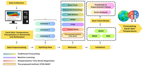
Figure 1. The framework architecture.

In addition, a dedicated visualization scheme was designed for the STSR-MASF model to illustrate the relationship between the predictor variables and the response variable. This schematic illustrates how each component, the parametric (autoregressive), nonparametric truncated spline, and nonparametric Fourier series, collectively contributes to the model’s overall structure. The architectural framework of the STSR-MASF model is presented in Figure 2.

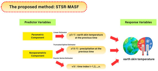
Figure 2. Overview of the STSR-MASF model structure and its components.

Based on Figure 2, Earth’s skin temperature at the previous time ($y_{t-1}$) was used as a predictor to account for the fact that Earth’s current skin temperature is influenced by previous conditions. Precipitation was included because rainfall can directly lower Earth’s skin temperature by increasing soil and air moisture and through evaporative cooling [43]. Rainfall is also part of the hydrological cycle, affecting how energy is distributed and influencing Earth’s short-term and seasonal skin temperature patterns [44,45]. By considering the order of observations over time, the STSR-MASF model can capture seasonal changes and variations in Earth’s skin temperature between periods, while also accounting for the two-way relationship between temperature and precipitation. This approach is consistent with tropical climatology, where Earth’s skin temperature and rainfall influence each other through processes like evapotranspiration and heat exchange between the surface and atmosphere.

Furthermore, the data-splitting procedure is explained in greater detail through three illustrative schemes, each clearly outlining the proportions of training and testing datasets. These visualizations, presented in Figure 3, provide a comprehensive overview of the experimental design implemented in this study.

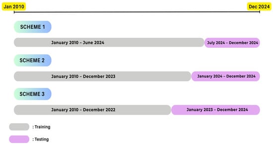
Figure 3. Data-splitting schemes.

The test sets were divided into durations of 0.5, 1, and 2 years to examine inter-seasonal variability in the tropical region, where seasonal changes typically occur twice a year, and to determine the most suitable training-testing scheme. This approach allows us to evaluate the capability of STSR-MASF in capturing seasonal patterns and producing reliable predictions over different periods.

3. Results

3.1. Exploratory Data Analysis

An exploratory analysis of Earth’s skin temperature data was conducted using time series plots and box plots to examine trends and seasonality. This initial exploration provides a comprehensive overview of the data characteristics prior to modeling. The visualizations are presented in Figure 4 and Figure 5.

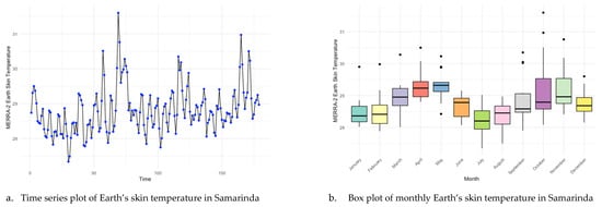
Figure 4. Exploratory visualization of Earth’s skin temperature data in Samarinda.

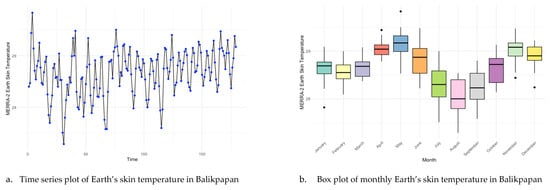
Figure 5. Exploratory visualization of Earth’s skin temperature data in Balikpapan.

The city of Samarinda exhibits a clear seasonal temperature pattern with noticeable fluctuations throughout the year. As shown in Figure 4a, the Earth’s skin temperature in Samarinda displays considerable variation, with several temperature spikes occurring in specific months, particularly from October to December. This period coincides with the dry season, which is typically characterized by higher temperatures. In addition, the graph shows a notable temperature increase during March and April, reflecting the transition from the rainy season to the dry season. This temperature rise is associated with reduced rainfall and increased solar radiation intensity, both of which contribute to the heating of the Earth’s skin temperature. Figure 4b further confirms this seasonal pattern, showing lower temperatures in January and February, corresponding to a cooler, more stable rainy season. In this case, higher-temperature outliers are frequently observed in October, November, and December, indicating temperature surges that are significantly higher than the usual monthly distributions. This phenomenon is likely influenced by climatic or extreme weather conditions that affect temperatures in Samarinda during the dry season. Overall, Samarinda’s temperature follows a consistent seasonal cycle, with peak temperatures toward the end of the year and lower temperatures at the beginning.

The city of Balikpapan, as shown in Figure 5a, demonstrates a temperature fluctuation pattern like that of Samarinda, although with smaller variations. Temperatures in Balikpapan tend to remain more stable throughout the year, but still exhibit a clear upward trend from October to December, indicating that these months, as in Samarinda, correspond to a hotter, drier season. Figure 5b shows a narrower temperature distribution during these months, reflecting more stable yet higher temperatures than in other periods. This pattern is associated with reduced rainfall and increased duration and intensity of solar radiation exposure. Meanwhile, January–March shows lower and more stable temperatures, corresponding to the rainy season. Higher temperature outliers in Balikpapan tend to occur in October and November, indicating more extreme temperature surges during these months, even though the city’s overall temperature remains relatively stable. This phenomenon may be attributed to climate variability or specific weather events that cause higher-than-usual temperatures, particularly during the peak of the dry season.

3.2. Application of STSR-MASF for Predictive Modeling

This section discusses the modeling process using STSR-MASF. Before the parameter estimation process, an initial visualization, in the form of a scatter plot, is performed to examine the relationship between time variables and Earth’ skin temperature values. This visualization helps us to identify the underlying nonlinear patterns and seasonal components of the data while also providing an initial overview of the data characteristics to be modeled by STSR-MASF.

3.2.1. Scatter Plots

Based on Figure 6 and Figure 7, the relationship between the Earth’s skin temperature at the previous time ($y_{t-1}$) and the current Earth’s skin temperature ($y_t$) in both Samarinda and Balikpapan exhibits a linear pattern. This indicates a linear temporal dependence, where the current Earth’s skin temperature is influenced by its previous value. This pattern represents the parametric component of the STSR-MASF model, which captures the direct dependence between past and present observations through the autoregressive (AR) component.

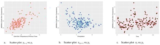
Figure 6. Scatter plots showing the relationship between Earth’s skin temperature and predictor variables in Samarinda.

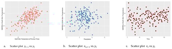
Figure 7. Scatter plots showing the relationship between Earth’s skin temperature and predictor variables in Balikpapan.

Meanwhile, the relationship between the previous precipitation ($z_{1,t-1}$) and the current Earth’s skin temperature ($y_t$) in both cities shows a random, irregular pattern, suggesting a nonlinear relationship that varies across subintervals. Therefore, this relationship is modeled using the truncated spline estimator, which represents the nonparametric component of the STSR-MASF and captures nonlinear variations in the data.

Furthermore, the relationship between time ($v_t$) and Earth’s skin temperature ($y_t$) exhibits a periodic pattern, indicating a seasonal component that recurs consistently. This pattern corresponds to the Fourier series component of the STSR-MASF model, which captures periodic or oscillatory behavior in the temperature data. Overall, the predictor variables used in this study reflect the three main components of the STSR-MASF model. Together, these components enable the model to effectively capture linear, nonlinear, and periodic patterns in the Earth’s skin temperature (y_t) data for both Samarinda and Balikpapan.

3.2.2. Implementation and Estimation Results of STSR-MASF

The implementation of the STSR-MASF model for the Earth’s skin temperature data in Samarinda and Balikpapan, using the predictor variables listed in Table 2, is presented in Table 3, Table 4 and Table 5. The STSR-MASF model consists of two main components: a parametric component and a nonparametric component, represented by the truncated spline estimator and the Fourier series, respectively.

In this study, the nonparametric truncated spline component was tested with one to three knot points and employed a linear order ($m=1$), while the nonparametric Fourier series component was tested with one to three oscillations. The linear order was chosen based on the principle of parsimony, aiming to use the simplest model that adequately captures the main trend in the temperature time series without unnecessary complexity. The knot locations in the STSR-MASF model were determined based on the observed values of the predictor variable. Specifically, the knots were placed by evenly dividing the range between the minimum and maximum values of the predictor. To avoid boundary effects, the first and last points of the range were excluded, ensuring that all knots were positioned strictly within the observed data.

The STSR-MASF models were then constructed through an iterative process that combined different numbers of knots in the truncated spline component with different numbers of oscillations in the Fourier series component. Each model configuration represented a distinct level of flexibility and complexity, reflecting the interaction between the model’s parametric and nonparametric structures. All candidate models were evaluated using the Generalized Cross-Validation (GCV) criterion. The optimal STSR-MASF model was selected based on the combination of knots and oscillations that produced the minimum GCV value. A lower GCV indicates a model with the smallest generalization error, implying the best predictive performance and the most appropriate representation of the true data pattern.

1.

Scheme 1

The summary of the STSR-MASF modeling results for Earth’s skin temperature data in Samarinda and Balikpapan under Scheme 1 is presented in Table 2. Knot indicates the number of truncated spline knots and Oscillation denotes the number of Fourier harmonics employed in the STSR–MASF model.

Table 2. Performance Evaluation of the STSR-MASF Model (Scheme 1).

Location	Knot	Oscillation		Training			Testing
			GCV	MSE	RMSE	MAPE (%)	MSE	RMSE	MAPE (%)
Samarinda	1	1	31.6959	0.1687	0.4107	1.1311	0.0524	0.2290	0.7308
		2	31.6067	0.1642	0.4052	1.1077	0.0480	0.2190	0.6368
		3	31.6937	0.1606	0.4008	1.1046	0.0685	0.2617	0.8268
	2	1	31.3572	0.1649	0.4061	1.1345	0.0543	0.2331	0.7307
		2	31.1917	0.1601	0.4001	1.1092	0.0562	0.2371	0.6385
		3	31.3925	0.1572	0.3964	1.1041	0.0583	0.2414	0.7752
	3	1	30.6725	0.1593	0.3992	1.1101	0.0860	0.2932	0.8797
		2	30.5395	0.1548	0.3934	1.0889	0.0857	0.2927	0.8705
		3	30.6733	0.1517	0.3894	1.0777	0.0874	0.2957	0.9015
Balikpapan	1	1	20.3468	0.1083	0.3291	0.9058	0.0851	0.2917	0.8732
		2	20.3768	0.1058	0.3253	0.9066	0.0956	0.3092	0.9671
		3	20.8774	0.1058	0.3253	0.9060	0.0927	0.3044	0.9463
	2	1	20.4780	0.1077	0.3281	0.9006	0.0859	0.2930	0.8771
		2	20.5623	0.1055	0.3248	0.9025	0.0948	0.3079	0.9599
		3	21.0732	0.1055	0.3248	0.9021	0.0931	0.3051	0.9475
	3	1	20.6831	0.1074	0.3278	0.8969	0.0852	0.2919	0.8756
		2	31.6959	0.1687	0.4107	1.1311	0.0524	0.2290	0.7308
		3	31.6067	0.1642	0.4052	1.1077	0.0480	0.2190	0.6368

Table 2. Performance Evaluation of the STSR-MASF Model (Scheme 1).

Location	Knot	Oscillation		Training			Testing
			GCV	MSE	RMSE	MAPE (%)	MSE	RMSE	MAPE (%)
Samarinda	1	1	31.6959	0.1687	0.4107	1.1311	0.0524	0.2290	0.7308
		2	31.6067	0.1642	0.4052	1.1077	0.0480	0.2190	0.6368
		3	31.6937	0.1606	0.4008	1.1046	0.0685	0.2617	0.8268
	2	1	31.3572	0.1649	0.4061	1.1345	0.0543	0.2331	0.7307
		2	31.1917	0.1601	0.4001	1.1092	0.0562	0.2371	0.6385
		3	31.3925	0.1572	0.3964	1.1041	0.0583	0.2414	0.7752
	3	1	30.6725	0.1593	0.3992	1.1101	0.0860	0.2932	0.8797
		2	30.5395	0.1548	0.3934	1.0889	0.0857	0.2927	0.8705
		3	30.6733	0.1517	0.3894	1.0777	0.0874	0.2957	0.9015
Balikpapan	1	1	20.3468	0.1083	0.3291	0.9058	0.0851	0.2917	0.8732
		2	20.3768	0.1058	0.3253	0.9066	0.0956	0.3092	0.9671
		3	20.8774	0.1058	0.3253	0.9060	0.0927	0.3044	0.9463
	2	1	20.4780	0.1077	0.3281	0.9006	0.0859	0.2930	0.8771
		2	20.5623	0.1055	0.3248	0.9025	0.0948	0.3079	0.9599
		3	21.0732	0.1055	0.3248	0.9021	0.0931	0.3051	0.9475
	3	1	20.6831	0.1074	0.3278	0.8969	0.0852	0.2919	0.8756
		2	31.6959	0.1687	0.4107	1.1311	0.0524	0.2290	0.7308
		3	31.6067	0.1642	0.4052	1.1077	0.0480	0.2190	0.6368

Based on the results presented in Table 2, the best STSR-MASF model for Scheme 1 in Samarinda achieved the minimum GCV value of 30.5395, obtained with a configuration of three knot points and two oscillations. The model showed good performance based on the accuracy measures from the training data. In Balikpapan, the best STSR-MASF model yielded the minimum GCV value of 20.3468 with a configuration of one knot point and one oscillation.

2.

Scheme 2

The summary of the STSR-MASF modeling results for Earth’s skin temperature data in Samarinda and Balikpapan under Scheme 2 is presented in Table 3. Knot indicates the number of truncated spline knots, and Oscillation denotes the number of Fourier harmonics employed in the STSR–MASF model.

Table 3. Performance evaluation of the STSR-MASF Model (Scheme 2).

Location	Knot	Oscillation		Training			Testing
			GCV	MSE	RMSE	MAPE (%)	MSE	RMSE	MAPE (%)
Samarinda	1	1	29.8223	0.1639	0.4049	1.1190	0.1812	0.4257	1.0365
		2	29.7107	0.1592	0.3991	1.0913	0.2090	0.4571	1.0904
		3	30.0631	0.1571	0.3963	1.0976	0.1711	0.4136	1.0028
	2	1	29.5259	0.1603	0.4003	1.1223	0.1786	0.4226	0.9800
		2	29.3183	0.1552	0.3939	1.0930	0.2167	0.4655	1.1142
		3	29.7933	0.1537	0.3920	1.0940	0.1771	0.4208	0.9425
	3	1	29.2917	0.1570	0.3962	1.1137	0.1715	0.4141	0.9131
		2	29.0081	0.1516	0.3893	1.0851	0.2113	0.4597	1.0730
		3	29.4829	0.1501	0.3875	1.0855	0.1689	0.4110	0.8706
Balikpapan	1	1	20.1900	0.1110	0.3331	0.9204	0.0633	0.2517	0.7293
		2	20.2017	0.1083	0.3291	0.9199	0.0828	0.2877	0.8406
		3	20.6956	0.1081	0.3288	0.9169	0.0981	0.3132	0.9151
	2	1	20.3238	0.1103	0.3321	0.9147	0.0641	0.2532	0.7326
		2	20.3980	0.1080	0.3286	0.9159	0.0808	0.2843	0.8270
		3	20.8981	0.1078	0.3283	0.9130	0.0972	0.3118	0.9091
	3	1	20.5398	0.1101	0.3318	0.9111	0.0636	0.2523	0.7315
		2	20.5915	0.1076	0.3280	0.9130	0.0837	0.2894	0.8480
		3	21.1173	0.1075	0.3279	0.9098	0.1028	0.3206	0.9349

Table 3. Performance evaluation of the STSR-MASF Model (Scheme 2).

Location	Knot	Oscillation		Training			Testing
			GCV	MSE	RMSE	MAPE (%)	MSE	RMSE	MAPE (%)
Samarinda	1	1	29.8223	0.1639	0.4049	1.1190	0.1812	0.4257	1.0365
		2	29.7107	0.1592	0.3991	1.0913	0.2090	0.4571	1.0904
		3	30.0631	0.1571	0.3963	1.0976	0.1711	0.4136	1.0028
	2	1	29.5259	0.1603	0.4003	1.1223	0.1786	0.4226	0.9800
		2	29.3183	0.1552	0.3939	1.0930	0.2167	0.4655	1.1142
		3	29.7933	0.1537	0.3920	1.0940	0.1771	0.4208	0.9425
	3	1	29.2917	0.1570	0.3962	1.1137	0.1715	0.4141	0.9131
		2	29.0081	0.1516	0.3893	1.0851	0.2113	0.4597	1.0730
		3	29.4829	0.1501	0.3875	1.0855	0.1689	0.4110	0.8706
Balikpapan	1	1	20.1900	0.1110	0.3331	0.9204	0.0633	0.2517	0.7293
		2	20.2017	0.1083	0.3291	0.9199	0.0828	0.2877	0.8406
		3	20.6956	0.1081	0.3288	0.9169	0.0981	0.3132	0.9151
	2	1	20.3238	0.1103	0.3321	0.9147	0.0641	0.2532	0.7326
		2	20.3980	0.1080	0.3286	0.9159	0.0808	0.2843	0.8270
		3	20.8981	0.1078	0.3283	0.9130	0.0972	0.3118	0.9091
	3	1	20.5398	0.1101	0.3318	0.9111	0.0636	0.2523	0.7315
		2	20.5915	0.1076	0.3280	0.9130	0.0837	0.2894	0.8480
		3	21.1173	0.1075	0.3279	0.9098	0.1028	0.3206	0.9349

Based on the results presented in Table 3, the best STSR-MASF model for Scheme 2 in Samarinda achieved the minimum GCV value of 29.0081, obtained with a configuration of three knot points and two oscillations. In Balikpapan, the best STSR-MASF model yielded the minimum GCV value of 20.1900 with a configuration of one knot point and one oscillation.

3.

Scheme 3

The summary of the STSR-MASF modeling results for Earth’s skin temperature data in Samarinda and Balikpapan under Scheme 3 is presented in Table 4. Knot indicates the number of truncated spline knots, and Oscillation denotes the number of Fourier harmonics employed in the STSR–MASF model.

Table 4. Performance Evaluation of the STSR-MASF Model (Scheme 3).

Location	Knot	Oscillation		Training			Testing
			GCV	MSE	RMSE	MAPE (%)	MSE	RMSE	MAPE (%)
Samarinda	1	1	26.9200	0.1583	0.3979	1.1087	0.2484	0.4984	1.1917
		2	26.3297	0.1507	0.3882	1.0742	0.5226	0.7229	1.8907
		3	27.0585	0.1507	0.3882	1.0750	0.4983	0.7059	1.8267
	2	1	26.8704	0.1559	0.3949	1.1020	0.2518	0.5018	1.1980
		2	26.2287	0.1481	0.3848	1.0709	0.5228	0.7230	1.8874
		3	26.9530	0.1480	0.3847	1.0712	0.5329	0.7300	1.9152
	3	1	26.6922	0.1528	0.3909	1.0983	0.2134	0.4620	1.0979
		2	25.9890	0.1447	0.3804	1.0574	0.1601	0.3996	1.0675
		3	26.7253	0.1447	0.3804	1.0577	0.5014	0.7081	1.8850
Balikpapan	1	1	19.1071	0.1124	0.3352	0.9193	0.0815	0.2855	0.8532
		2	19.1018	0.1093	0.3307	0.9163	0.0975	0.3122	0.9289
		3	19.5013	0.1086	0.3295	0.9160	0.1477	0.3844	1.0874
	2	1	19.2413	0.1117	0.3341	0.9137	0.0828	0.2877	0.8547
		2	19.3062	0.1090	0.3302	0.9124	0.0969	0.3113	0.9237
		3	19.7031	0.1082	0.3289	0.9119	0.1494	0.3865	1.0913
	3	1	19.5169	0.1117	0.3342	0.9090	0.0821	0.2865	0.8611
		2	19.3190	0.1076	0.3280	0.9048	0.1068	0.3267	0.9776
		3	19.9134	0.1078	0.3284	0.9042	0.1508	0.3884	1.1024

Table 4. Performance Evaluation of the STSR-MASF Model (Scheme 3).

Location	Knot	Oscillation		Training			Testing
			GCV	MSE	RMSE	MAPE (%)	MSE	RMSE	MAPE (%)
Samarinda	1	1	26.9200	0.1583	0.3979	1.1087	0.2484	0.4984	1.1917
		2	26.3297	0.1507	0.3882	1.0742	0.5226	0.7229	1.8907
		3	27.0585	0.1507	0.3882	1.0750	0.4983	0.7059	1.8267
	2	1	26.8704	0.1559	0.3949	1.1020	0.2518	0.5018	1.1980
		2	26.2287	0.1481	0.3848	1.0709	0.5228	0.7230	1.8874
		3	26.9530	0.1480	0.3847	1.0712	0.5329	0.7300	1.9152
	3	1	26.6922	0.1528	0.3909	1.0983	0.2134	0.4620	1.0979
		2	25.9890	0.1447	0.3804	1.0574	0.1601	0.3996	1.0675
		3	26.7253	0.1447	0.3804	1.0577	0.5014	0.7081	1.8850
Balikpapan	1	1	19.1071	0.1124	0.3352	0.9193	0.0815	0.2855	0.8532
		2	19.1018	0.1093	0.3307	0.9163	0.0975	0.3122	0.9289
		3	19.5013	0.1086	0.3295	0.9160	0.1477	0.3844	1.0874
	2	1	19.2413	0.1117	0.3341	0.9137	0.0828	0.2877	0.8547
		2	19.3062	0.1090	0.3302	0.9124	0.0969	0.3113	0.9237
		3	19.7031	0.1082	0.3289	0.9119	0.1494	0.3865	1.0913
	3	1	19.5169	0.1117	0.3342	0.9090	0.0821	0.2865	0.8611
		2	19.3190	0.1076	0.3280	0.9048	0.1068	0.3267	0.9776
		3	19.9134	0.1078	0.3284	0.9042	0.1508	0.3884	1.1024

Based on the results presented in Table 4, the best STSR-MASF model for Scheme 3 in Samarinda achieved the minimum GCV value of 25.9890, obtained with a configuration of three knot points and two oscillations. In Balikpapan, the best STSR-MASF model yielded the minimum GCV value of 19.1018 with a configuration of one knot point and two oscillations.

Table 5. Final selected benchmark models and optimal parameters for each location and scheme.

Location	Scheme	Exponential Smoothing	Holt-Winters	SARIMA	FFNN	Fourier Series
Samarinda	1	$\alpha =0.1$	$\alpha =0.7358$ $\rho =0.0218$ $\kappa =0.4080$	SARIMA (4,1,0)(1,1,0)6	Best NN architecture: 5 neurons (HL1), 2 neurons (HL2)	3 oscillations
	2	$\alpha =0.1$	$\alpha =0.7466$ $\rho =0.0219$ $\kappa =0.4303$	SARIMA (4,1,0)(1,1,0)6	Best NN architecture: 1 neuron (HL1), 5 neurons (HL2)	3 oscillations
	3	$\alpha =0.9$	$\alpha =0.7145$ $\rho =0.0241$ $\kappa =0.7467$	SARIMA (4,1,0)(1,1,0)6	Best NN architecture: 5 neurons (HL1), 4 neurons (HL2)	3 oscillations
Balikpapan	1	$\alpha =0.1$	$\alpha =0.8217$ $\rho =0.0127$ $\kappa =1.0000$	SARIMA (4,1,0)(1,1,0)6	Best NN architecture: 1 neuron (HL1), 3 neurons (HL2)	2 oscillations
	2	$\alpha =0.3$	$\alpha =0.8183$ $\rho =0.0132$ $\kappa =1.0000$	SARIMA (4,1,0)(1,1,0)6	Best NN architecture: 1 neuron (HL1), 5 neurons (HL2)	2 oscillations
	3	$\alpha =0.3$	$\alpha =0.8159$ $\rho =0.0127$ $\kappa =1.0000$	SARIMA (4,1,0)(1,1,0)6	Best NN architecture: 1 neuron (HL1), 5 neurons (HL2)	2 oscillations

Table 5. Final selected benchmark models and optimal parameters for each location and scheme.

Location	Scheme	Exponential Smoothing	Holt-Winters	SARIMA	FFNN	Fourier Series
Samarinda	1	$\alpha =0.1$	$\alpha =0.7358$ $\rho =0.0218$ $\kappa =0.4080$	SARIMA (4,1,0)(1,1,0)6	Best NN architecture: 5 neurons (HL1), 2 neurons (HL2)	3 oscillations
	2	$\alpha =0.1$	$\alpha =0.7466$ $\rho =0.0219$ $\kappa =0.4303$	SARIMA (4,1,0)(1,1,0)6	Best NN architecture: 1 neuron (HL1), 5 neurons (HL2)	3 oscillations
	3	$\alpha =0.9$	$\alpha =0.7145$ $\rho =0.0241$ $\kappa =0.7467$	SARIMA (4,1,0)(1,1,0)6	Best NN architecture: 5 neurons (HL1), 4 neurons (HL2)	3 oscillations
Balikpapan	1	$\alpha =0.1$	$\alpha =0.8217$ $\rho =0.0127$ $\kappa =1.0000$	SARIMA (4,1,0)(1,1,0)6	Best NN architecture: 1 neuron (HL1), 3 neurons (HL2)	2 oscillations
	2	$\alpha =0.3$	$\alpha =0.8183$ $\rho =0.0132$ $\kappa =1.0000$	SARIMA (4,1,0)(1,1,0)6	Best NN architecture: 1 neuron (HL1), 5 neurons (HL2)	2 oscillations
	3	$\alpha =0.3$	$\alpha =0.8159$ $\rho =0.0127$ $\kappa =1.0000$	SARIMA (4,1,0)(1,1,0)6	Best NN architecture: 1 neuron (HL1), 5 neurons (HL2)	2 oscillations

3.3. Modeling with Naïve Trend, Exponential Smoothing, Holt-Winters, ARIMA, FFNN, and Fourier Series

This section models Earth’s skin temperature data using three methodological categories. First, classical statistical methods are applied, including Naïve Trend, Exponential Smoothing, additive Holt–Winters, and ARIMA models. Next, the nonparametric approach is represented by the Fourier Series. Finally, the machine learning method employs a feed-forward neural network (FFNN). Taken together, these methods provide comparative baselines for evaluating the proposed STSR-MASF model.

• Naïve Trend
  The Naïve Trend method assumes that the change between the last two observations persists at a constant rate into the subsequent period. Forecasts are generated by adding the difference between the two most recent values to the latest observation. This approach is effective for datasets exhibiting a stable trend.
• Exponential Smoothing
  The exponential smoothing method employs a single smoothing parameter, the level constant ($\alpha$), which assigns greater weight to more recent observations and allows for the model to adapt to recent changes. In this study, the smoothing parameter α was examined over a grid of candidate values ranging from 0.1 to 0.9 with an increment of 0.1. The optimal value of $\alpha$ was selected by minimizing forecast error measures, and is reported in Table 5.
• Holt–Winters
  The additive Holt–Winters method captures relatively constant trend and seasonal patterns over time. This method uses three parameters: level ($\alpha$), trend ($\rho$), and seasonal ($\kappa$). These are combined additively if seasonal variations have constant amplitude across periods. The values of $\alpha$, $\rho$, and $\kappa$ are tuned to achieve the most accurate forecasts. Model performance is evaluated using MSE, RMSE, and MAPE. The additive Holt–Winters models were estimated using the HoltWinters() function in R. The level (α), trend ($\rho$), and seasonal ($\kappa$) smoothing parameters were automatically optimized by minimizing the sum of squared errors. The final estimated smoothing parameters for each city and scheme are explicitly reported in Table 5 to ensure fairness and reproducibility in comparison with the proposed STSR–MASF model.
• ARIMA
  The ARIMA modeling process starts by examining the data’s characteristics, especially stationarity of the variance and the mean. Variance stationarity is assessed with the Box–Cox transformation. Mean stationarity is evaluated visually using the Autocorrelation Function (ACF) plot. After confirming stationarity, patterns of autocorrelation and partial autocorrelation, identified using the Autocorrelation Function (ACF) and Partial Autocorrelation Function (PACF), are analyzed. These analyses indicate a seasonal component with a period of six. Consequently, a Seasonal Autoregressive Integrated Moving Average (SARIMA) model, denoted as (p, d, q)(P, D, Q)_s, is employed. For each scheme and city, model selection involves evaluating all possible SARIMA parameter combinations, namely SARIMA (1,1,0)(1,1,0)₆, SARIMA (2,1,0)(1,1,0)₆, SARIMA (3,1,0)(1,1,0)₆, and SARIMA (4,1,0)(1,1,0)₆. The optimal model is selected based on three criteria: parameter significance, independence of residuals as assessed by the Ljung–Box test, and normality of residuals as determined by the Kolmogorov–Smirnov test. Some of the best SARIMA models do not fully satisfy the residual independence assumption for certain schemes and cities. Based on the evaluation criteria and forecasting performance, the SARIMA (4,1,0)(1,1,0)₆ model is consistently identified as the optimal specification across all schemes and cities and is therefore selected as the final SARIMA benchmark model in this study.
• FFNN
  The FFNN modeling process was implemented in R using the neuralnet package. The FFNN modeling process starts by selecting input variables from time-lagged observations. ACF and PACF analyses of the training data help identify the relevant lags for each scheme and city: $y_{t-1}$ and $y_{t-2}$. The FFNN architecture has two Hidden Layers (HL), with 1–8 neurons per layer. The optimal configuration is identified using evaluation metrics MSE, RMSE, and MAPE. The model was trained using the backpropagation algorithm with mean squared error (MSE) as the loss function. The activation function for hidden neurons was the logistic function, while the output layer used a linear activation. Data are standardized using min–max normalization to ensure stable convergence and accelerate learning.
• Fourier Series
  The Fourier Series approach captures periodic patterns in the data using sine and cosine functions. Models with one to three oscillations are evaluated. The optimal model is selected based on the minimum Generalized Cross Validation (GCV) value, which balances model complexity and estimation error.

3.4. Performance Comparison of STSR-MASF and Benchmark Forecasting Methods

Seven time series modeling methods were evaluated using Earth’s skin temperature data from Samarinda and Balikpapan across three observation schemes. The goal was to assess how well each method captured data patterns, including trends, seasonality, and random fluctuations. Model accuracy was assessed with MSE, RMSE, and MAPE on training and test sets. Lower errors indicate more accurate estimations and forecasts. Table 6, Table 7 and Table 8 present complete modeling results for each method, scheme, and location, summarizing the model accuracy and best performers for every combination.

• Scheme 1

Table 6. Model performance comparison across seven time series approach for Scheme 1.

Location	Methods	Training			Testing
		MSE	RMSE	MAPE (%)	MSE	RMSE	MAPE (%)
Samarinda	Naïve Trend	0.4765	0.6903	1.8719	16.8412	4.1038	12.2744
	Exponential Smoothing	0.3918	0.6260	1.6408	0.2172	0.4660	1.2625
	Holt-Winters	0.3015	0.5491	1.4993	0.2588	0.5087	1.6310
	SARIMA	0.2414	0.4914	1.3558	0.1328	0.4622	1.2359
	FFNN	0.2080	0.4561	1.2236	0.1350	0.3674	1.1200
	Fourier Series	0.3438	0.5863	1.5547	0.1858	0.4300	1.2294
	STSR-MASF	0.1548	0.3934	1.0889	0.0857	0.2927	0.8705
Balikpapan	Naïve Trend	0.2195	0.4685	1.3189	1.0350	1.0173	2.8112
	Exponential Smoothing	0.1897	0.4355	1.2120	0.1242	0.3525	1.0497
	Holt-Winters	0.1383	0.3719	1.0611	0.1229	0.3506	1.1800
	SARIMA	0.2097	0.4579	1.2000	0.1799	0.4242	1.3445
	FFNN	0.2021	0.4496	1.2600	0.1596	0.3995	1.1300
	Fourier Series	0.1706	0.4131	1.1603	0.1255	0.3542	1.0459
	STSR-MASF	0.1083	0.3291	0.9058	0.0851	0.2917	0.8732

Table 6. Model performance comparison across seven time series approach for Scheme 1.

Location	Methods	Training			Testing
		MSE	RMSE	MAPE (%)	MSE	RMSE	MAPE (%)
Samarinda	Naïve Trend	0.4765	0.6903	1.8719	16.8412	4.1038	12.2744
	Exponential Smoothing	0.3918	0.6260	1.6408	0.2172	0.4660	1.2625
	Holt-Winters	0.3015	0.5491	1.4993	0.2588	0.5087	1.6310
	SARIMA	0.2414	0.4914	1.3558	0.1328	0.4622	1.2359
	FFNN	0.2080	0.4561	1.2236	0.1350	0.3674	1.1200
	Fourier Series	0.3438	0.5863	1.5547	0.1858	0.4300	1.2294
	STSR-MASF	0.1548	0.3934	1.0889	0.0857	0.2927	0.8705
Balikpapan	Naïve Trend	0.2195	0.4685	1.3189	1.0350	1.0173	2.8112
	Exponential Smoothing	0.1897	0.4355	1.2120	0.1242	0.3525	1.0497
	Holt-Winters	0.1383	0.3719	1.0611	0.1229	0.3506	1.1800
	SARIMA	0.2097	0.4579	1.2000	0.1799	0.4242	1.3445
	FFNN	0.2021	0.4496	1.2600	0.1596	0.3995	1.1300
	Fourier Series	0.1706	0.4131	1.1603	0.1255	0.3542	1.0459
	STSR-MASF	0.1083	0.3291	0.9058	0.0851	0.2917	0.8732

Comparing seven time series modeling methods on Earth’s skin temperature data from Samarinda and Balikpapan shows clear differences in fit. Notably, combining a truncated spline with a Fourier series enables the model to capture temporal patterns and variability more effectively than other approaches, indicating strong generalization and stability. Under Scheme 1, STSR–MASF performs well in both training and test sets.

2.

Scheme 2

Table 7. Model performance comparison across seven time series approach for Scheme 2.

Location	Methods	Training			Testing
		MSE	RMSE	MAPE (%)	MSE	RMSE	MAPE (%)
Samarinda	Naïve Trend	0.4661	0.6827	1.8467	33.2973	5.7704	17.5157
	Exponential Smoothing	0.3896	0.6242	1.6399	0.3269	0.5717	1.4315
	Holt-Winters	0.2967	0.5447	1.4941	0.2547	0.5046	1.5365
	SARIMA	0.2344	0.4841	1.3437	1.0332	1.0165	3.1229
	FFNN	0.3616	0.6013	1.5500	0.5885	0.7671	1.9100
	Fourier Series	0.3410	0.5840	1.5463	0.4154	0.6445	1.4206
	STSR-MASF	0.1516	0.3893	1.0851	0.2113	0.4597	1.0730
Balikpapan	Naïve Trend	0.2234	0.4726	1.3336	4.8959	2.2127	6.5134
	Exponential Smoothing	0.1874	0.4329	1.2345	0.0905	0.3009	0.8008
	Holt-Winters	0.1393	0.3732	1.0630	0.1245	0.3528	0.9650
	SARIMA	0.1813	0.4258	1.1190	0.0902	0.3003	0.9028
	FFNN	0.2032	0.4508	1.2600	0.1648	0.4060	1.2200
	Fourier Series	0.1746	0.4178	1.1770	0.1175	0.3428	1.0004
	STSR-MASF	0.1110	0.3331	0.9204	0.0633	0.2517	0.7293

Table 7. Model performance comparison across seven time series approach for Scheme 2.

Location	Methods	Training			Testing
		MSE	RMSE	MAPE (%)	MSE	RMSE	MAPE (%)
Samarinda	Naïve Trend	0.4661	0.6827	1.8467	33.2973	5.7704	17.5157
	Exponential Smoothing	0.3896	0.6242	1.6399	0.3269	0.5717	1.4315
	Holt-Winters	0.2967	0.5447	1.4941	0.2547	0.5046	1.5365
	SARIMA	0.2344	0.4841	1.3437	1.0332	1.0165	3.1229
	FFNN	0.3616	0.6013	1.5500	0.5885	0.7671	1.9100
	Fourier Series	0.3410	0.5840	1.5463	0.4154	0.6445	1.4206
	STSR-MASF	0.1516	0.3893	1.0851	0.2113	0.4597	1.0730
Balikpapan	Naïve Trend	0.2234	0.4726	1.3336	4.8959	2.2127	6.5134
	Exponential Smoothing	0.1874	0.4329	1.2345	0.0905	0.3009	0.8008
	Holt-Winters	0.1393	0.3732	1.0630	0.1245	0.3528	0.9650
	SARIMA	0.1813	0.4258	1.1190	0.0902	0.3003	0.9028
	FFNN	0.2032	0.4508	1.2600	0.1648	0.4060	1.2200
	Fourier Series	0.1746	0.4178	1.1770	0.1175	0.3428	1.0004
	STSR-MASF	0.1110	0.3331	0.9204	0.0633	0.2517	0.7293

Modeling results under Scheme 2 confirm that STSR–MASF continues to achieve the highest accuracy at both sites. The consistently low errors indicate that the model effectively reflects Earth’s skin temperature dynamics and sustains high generalization. Overall, under Scheme 2, STSR–MASF demonstrates the most reliable performance among the seven methods.

3.

Scheme 3

Table 8. Model performance comparison across seven time series approach for Scheme 3.

Location	Methods	Training			Testing
		MSE	RMSE	MAPE (%)	MSE	RMSE	MAPE (%)
Samarinda	Naïve Trend	0.4685	0.6845	1.8622	1.3337	1.1548	3.1527
	Exponential Smoothing	0.2763	0.5257	1.3715	0.3481	0.5900	1.5798
	Holt-Winters	0.3175	0.5635	1.5283	1.1249	1.0606	3.1227
	SARIMA	0.2331	0.4828	1.3285	0.8275	0.9096	2.2005
	FFNN	0.2349	0.4846	1.2700	0.6755	0.8219	1.9000
	Fourier Series	0.3141	0.5604	1.5135	0.9323	0.9656	2.4681
	STSR-MASF	0.1447	0.3804	1.0574	0.1601	0.3996	1.0675
Balikpapan	Naïve Trend	0.2296	0.4792	1.3523	1.6523	1.2854	3.6939
	Exponential Smoothing	0.1903	0.4362	1.2404	0.1195	0.3456	0.9639
	Holt-Winters	0.1416	0.3763	1.0749	0.1450	0.3808	1.1100
	SARIMA	0.1784	0.4224	1.1094	0.0521	0.2282	2.6346
	FFNN	0.2054	0.4533	1.2700	0.1806	0.4249	1.2400
	Fourier Series	0.1773	0.4211	1.1772	0.1512	0.3888	1.1332
	STSR-MASF	0.1093	0.3307	0.9163	0.0975	0.3122	0.9289

Table 8. Model performance comparison across seven time series approach for Scheme 3.

Location	Methods	Training			Testing
		MSE	RMSE	MAPE (%)	MSE	RMSE	MAPE (%)
Samarinda	Naïve Trend	0.4685	0.6845	1.8622	1.3337	1.1548	3.1527
	Exponential Smoothing	0.2763	0.5257	1.3715	0.3481	0.5900	1.5798
	Holt-Winters	0.3175	0.5635	1.5283	1.1249	1.0606	3.1227
	SARIMA	0.2331	0.4828	1.3285	0.8275	0.9096	2.2005
	FFNN	0.2349	0.4846	1.2700	0.6755	0.8219	1.9000
	Fourier Series	0.3141	0.5604	1.5135	0.9323	0.9656	2.4681
	STSR-MASF	0.1447	0.3804	1.0574	0.1601	0.3996	1.0675
Balikpapan	Naïve Trend	0.2296	0.4792	1.3523	1.6523	1.2854	3.6939
	Exponential Smoothing	0.1903	0.4362	1.2404	0.1195	0.3456	0.9639
	Holt-Winters	0.1416	0.3763	1.0749	0.1450	0.3808	1.1100
	SARIMA	0.1784	0.4224	1.1094	0.0521	0.2282	2.6346
	FFNN	0.2054	0.4533	1.2700	0.1806	0.4249	1.2400
	Fourier Series	0.1773	0.4211	1.1772	0.1512	0.3888	1.1332
	STSR-MASF	0.1093	0.3307	0.9163	0.0975	0.3122	0.9289

The comparison results in Scheme 3 again indicate that the STSR–MASF model performs better than the six other benchmark methods across both observation sites. For Scheme 3, STSR–MASF achieves the lowest training and testing errors in both Samarinda and Balikpapan. The model demonstrates stable performance and accuracy across both cities. Overall, the findings in Scheme 3 strengthen previous evidence that the STSR–MASF model exhibits strong adaptability and generalization ability in time series modeling.

4. Discussion

The STSR–MASF, a new statistical approach to forecasting Earth’s skin temperature based on MERRA-2, demonstrates promising performance across various evaluation schemes. This study is primarily methodological in nature, aiming to introduce the STSR-MASF approach as a statistical time series regression tool, focusing on its statistical development and an initial demonstration using climate-related data. Based on the results from both the training and testing datasets, all STSR–MASF configurations yielded relatively small and stable error values in the two observation areas: Samarinda and Balikpapan City. This finding indicates that the proposed model effectively captures the dynamic patterns and fluctuations of Earth’s skin temperature over time.

To identify the overall best-performing scheme, a comparative assessment was conducted. This assessment was based on the average MSE, RMSE, and MAPE values from the testing data of both locations. This approach was used because this study aimed to obtain a model configuration that is consistent and accurate across different regions, rather than one that performs optimally in only one location. The average testing performance for both cities is illustrated in Figure 8.

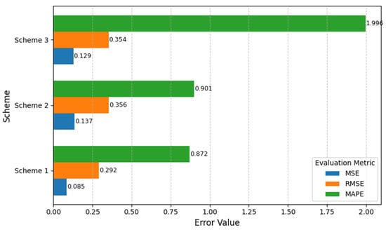
Figure 8. Average testing errors of the STSR–MASF schemes for Samarinda and Balikpapan.

Based on Figure 8, Scheme 1 produced the smallest average values of MSE, RMSE, and MAPE compared to the other two schemes, indicating that Scheme 1 represents the most optimal configuration of the STSR–MASF model. It provides the highest predictive accuracy during the testing phase across both locations and maintains stable performance between training and testing results. Furthermore, the MAPE value obtained under Scheme 1 is less than 10%, which, according to common forecasting standards, indicates a highly accurate prediction. The optimal STSR-MASF model for Scheme 1 in Samarinda is presented in Equation (31),

$$\begin{array}{cc}\hfill {\widehat{y}}_t=31.7023+0.532& y_{t-1}-0.782z_{1,t-1}+1.751{\left(z_{1,t-1}-3.138\right)}_{+}-1.437{\left(z_{1,t-1}-3.744\right)}_{+}+0.452{\left(z_{1,t-1}-4.956\right)}_{+}-0.000v_t\hfill \\ & +0.024\cos \left(2\pi \left({\displaystyle \frac{v_t-1}{n}}\right)\right)-0.100\sin \left(2\pi \left({\displaystyle \frac{v_t-1}{n}}\right)\right)+0.047\cos \left(4\pi \left({\displaystyle \frac{v_t-1}{n}}\right)\right)-0.113\sin \left(4\pi \left({\displaystyle \frac{v_t-1}{n}}\right)\right) ,\hfill \end{array}$$

(31)

while the corresponding model for Balikpapan is given in Equation (32):

$${\widehat{y}}_t=20.196+0.650y_{t-1}-0.014z_{1,t-1}+0.826{\left(z_{1,t-1}-15.444\right)}_{+}+0.000v_t+0.038\cos \left(2\pi \left({\displaystyle \frac{v_t-1}{n}}\right)\right)-0.051\sin \left(2\pi \left({\displaystyle \frac{v_t-1}{n}}\right)\right)$$

(32)

Based on Figure 9, the testing MAPE values for all forecasting methods evaluated in this study are compared. The results show that the proposed STSR-MASF model attains a lower MAPE than the other methods, with detailed numerical values summarized in Table 6. This observation provides additional indication that the proposed approach can capture nonlinear patterns, seasonal behavior, and autoregressive dependencies in the data, resulting in a highly accurate prediction on the testing dataset. Although the MAPE value indicates a highly accurate prediction, examining the patterns of increase and decrease remains essential to understand how the model responds to real-world dynamics of Earth’s skin temperature.

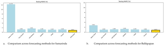
Figure 9. MAPE-based comparison of forecasting models on the testing dataset under Scheme 1.

In this study, an additional 11-month forecast was performed outside the testing step-by-step process to evaluate the model’s accuracy in predicting future temperatures. This extension was carried out by utilizing the parameters obtained from the STSR–MASF model under Scheme 1 and applying them sequentially from January 2025 to November 2025. The purpose of this additional forecast was to assess how well the model could predict temperatures for a period extending beyond the original testing data. By comparing the predicted values with the actual data as it becomes available, we can better evaluate the model’s predictive performance. The forecasting process was carried out sequentially, starting from January 2025, by substituting the previous temperature value ($y_{t-1}$), the data from December 2024, into the parametric component. For the truncated spline component, the previous precipitation value ($z_{1,t-1}$) from December 2024 was used, while the Fourier component was generated by substituting the time index $t=181$, corresponding to the next time step in the sequence. By substituting these three components into the STSR–MASF model equation, the estimated Earth’s skin temperature for January 2025 was obtained. The same procedure was then applied iteratively for subsequent periods up to November 2025. This forecasting horizon is limited to November because the STSR–MASF model operates as a short-term forecasting approach. Each new prediction must be informed by the most recent available observation, most notably being the previous precipitation value that feeds into the nonparametric truncated spline component. The forecasting results for Samarinda City and Balikpapan City are presented in Figure 10.

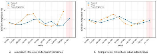
Figure 10. Step-by-step forecasting results of the STSR–MASF model.

The forecasting results were validated by comparing the model’s estimated values with actual data obtained from the official NASA POWER website (https://power.larc.nasa.gov) for two observation sites: Samarinda and Balikpapan. From the evaluation side, using MSE, RMSE, and MAPE on the forecasting data for the period January–October 2025, during which NASA POWER observational data were available, allowed for direct comparison with the STSR–MASF forecasts. These results further strengthen the earlier findings. When the model’s forecasts were compared with the corresponding validated observational data, the STSR–MASF model achieved an MSE of 0.3970, RMSE of 0.6300, and MAPE of 1.5917% for Samarinda. For Balikpapan, the error metrics were even smaller, with an MSE of 0.0978, RMSE of 0.3128, and MAPE of 0.9666%. The relatively low values across all indicators demonstrate the model’s strong ability to reproduce actual temperature variations, underscoring the close agreement between the predicted and observed Earth’s skin temperature in both cities. For November 2025, the actual observational data from NASA POWER were not yet available at the time of this analysis. Nevertheless, the STSR–MASF forecasts suggest a potential increase in temperature in both cities, aligning with the general warming tendency commonly observed toward the end of the year.

The STSR–MASF model not only delivers accurate predictions, but also introduces an innovative statistical framework. It integrates semiparametric regression with a mixed estimator that combines spline and Fourier series components. This enables the model to capture nonlinear patterns and underlying seasonal oscillations in the data. This approach provides a more comprehensive understanding of Earth’s skin temperature behavior than conventional methods typically offer. The primary strength of this study lies in both its forecasting outcomes and its conceptual and methodological innovation. The successful application of the STSR–MASF model to temperature dynamics in Samarinda and Balikpapan demonstrates the potential for statistical approaches to effectively represent natural phenomena.

5. Conclusions

We introduce the STSR–MASF model, a novel and effective approach to statistical time series analysis. By integrating a clear, flexible structure with advanced spline methods for smooth nonlinear trends and a Fourier element for recurring patterns, the STSR–MASF model sets a new standard in forecasting accuracy for cycles and seasonal effects. This innovation also yields six Lemmas and two Theorems that represent the mathematical foundation of the development. Empirical evaluations across multiple experiments show that the STSR–MASF model consistently provides more accurate and stable forecasts compared to six previous methods proposed in earlier studies. The model achieves lower MSE, RMSE, and MAPE values, while effectively capturing the temporal dynamics and fluctuations of Earth’s skin temperature in an adaptive, additive manner that responds to environmental variability. These results show that the STSR–MASF model is a strong tool for climate monitoring, energy planning, and environmental policy, especially in tropical places like Indonesia. In practice, the model’s insights can help city planners develop targeted cooling strategies for neighborhoods most affected by urban heat islands and assist energy providers in optimizing resource allocation during high temperature variability. For example, policymakers could use these short-term forecasts to adjust, such as improving energy distribution systems for the upcoming month or adding temporary green spaces and heat-resilient infrastructure to manage the immediate impact of heat.

Future research may extend the STSR–MASF framework to multipredictor formulations and explore mixed estimation strategies, such as spline–kernel or kernel–Fourier approaches, to better accommodate the complexity of climatic time series. Although the present study restricts the spline component to precipitation as a single explanatory variable, it is well established that other climatic drivers, including solar radiation, also play an important role in modulating temperature variability. The focus on a single predictor is intentionally adopted to highlight precipitation–temperature coupling and to preserve a coherent modeling structure in which each estimator is constructed based on one explanatory variable. Accordingly, incorporating additional predictors, such as solar radiation and other atmospheric variables, represents a natural extension of the proposed framework and is expected to further improve both model interpretability and forecasting accuracy.

References

- Wei, W.W.S. Time Series Analysis: Univariate and Multivariate Methods, 2nd ed.; Pearson Education, Inc.: New York, NY, USA, 2006. [Google Scholar]
- Chen, M.; Papadikis, K.; Jun, C.; Macdonald, N. Linear, nonlinear, parametric and nonparametric regression models for nonstationary flood frequency analysis. J. Hydrol. 2023, 616, 128772. [Google Scholar] [CrossRef]
- Chamidah, N.; Lestari, B.; Budiantara, I.N.; Aydin, D. Estimation of Multiresponse Multipredictor Nonparametric Regression Model Using Mixed Estimator. Symmetry 2024, 16, 386. [Google Scholar] [CrossRef]
- Wahba. Spline Models for Observational Data, 2nd ed.; SIAM: Philadelphia, PA, USA, 1990. [Google Scholar]
- Eubank, R.L.; Speckman, P.L. Confidence bands in nonparametric regression. J. Am. Stat. Assoc. 1993, 88, 1287–1301. [Google Scholar] [CrossRef]
- Gao, J. Nonlinear Time Series Semiparametric and Nonparametric Methods, 1st ed.; Chapman & Hall: London, UK; CRC: New York, NY, USA, 2007. [Google Scholar]
- Ratnasari, V.; Budiantara, I.N.; Dani, A.T.R. Nonparametric Regression Mixed Estimators of Truncated Spline and Gaussian Kernel based on Cross-Validation (CV), Generalized Cross- Validation (GCV), and Unbiased Risk (UBR) Methods. Int. J. Adv. Sci. Eng. Inf. Technol. 2021, 11, 2400–2406. [Google Scholar] [CrossRef]
- Eilers, P.H.C.; Marx, B.D. Splines, Knots, and Penalties. Wiley Interdiscip. Rev. Comput. Stat. 2010, 2, 637–653. [Google Scholar] [CrossRef]
- Regier, M.D.; Parker, R.D. Smoothing using fractional polynomials: An alternative to polynomials and splines in applied research. Wiley Interdiscip. Rev. Comput. Stat. 2015, 7, 275–283. [Google Scholar] [CrossRef]
- Budiantara, I.N.; Ratnasari, V.; Ratna, M.; Zain, I. The Combination of Spline and Kernel Estimator for Nonparametric Regression and its Properties. Appl. Math. Sci. 2015, 9, 6083–6094. [Google Scholar] [CrossRef]
- Bilodeau, M. Fourier smoother and additive models. Can. J. Stat. 1992, 20, 257–269. [Google Scholar] [CrossRef]
- Alabdally, H.; Ali, M.; Diykh, M.; Deo, R.C.; Aldhafeeri, A.A.; Abdulla, S.; Farooque, A.A. Improving Dry-Bulb Air Temperature Prediction Using a Hybrid Model Integrating Genetic Algorithms with a Fourier–Bessel Series Expansion-Based LSTM Model. Forecasting 2025, 7, 46. [Google Scholar] [CrossRef]
- Greblicki, W.; Pawlak, M. Fourier and Hermite series estimates of regression functions. Ann. Inst. Stat. Math. 1985, 37, 443–454. [Google Scholar] [CrossRef]
- Chu, C.-K.; Marron, J.S. Choosing a Kernel Regression Estimator. Stat. Sci. 1991, 6, 404–436. [Google Scholar] [CrossRef]
- Cui, W.; Wei, M. Strong Consistency of Kernel Regression Estimate. Open J. Stat. 2013, 3, 179–182. [Google Scholar] [CrossRef]
- Hartt, J.D. Kernel Regression Estimation with Time Series Errors. R. Stat. Soc. 1991, 53, 173–187. [Google Scholar] [CrossRef]
- Lestari, B.; Chamidah, N.; Budiantara, I.N.; Aydin, D. Determining confidence interval and asymptotic distribution for parameters of multiresponse semiparametric regression model using smoothing spline estimator. J. King Saud. Univ. Sci. 2023, 35, 102664. [Google Scholar] [CrossRef]
- Panchuk, K.; Myasoedova, T.; Lyubchinov, E. Spline curves formation given extreme derivatives. Mathematics 2021, 9, 47. [Google Scholar] [CrossRef]
- Ming, W.Y.; Huang, L.-J. Fourier Series Neural Networks for Regression. In Proceedings of the IEEE International Conference on Applied System Innovation, Chiba, Japan, 13–17 April 2018; IEEE: New York, NY, USA, 2018; pp. 716–719. [Google Scholar]
- Bloomfield, P. Fourier Analysis of Time Series An Introduction, 2nd ed.; John Wiley & Sons, Inc.: Toronto, ON, Canada, 2000. [Google Scholar]
- Chamidah, N.; Febriana, S.D.; Ariyanto, R.A.; Sahawaly, R. Fourier series estimator for predicting international market price of white sugar. In AIP Conference Proceedings; American Institute of Physics Inc.: College Park, MD, USA, 2021. [Google Scholar] [CrossRef]
- Ratnasari, V.; Budiantara, I.N.; Ratna, M.; Zain, I. Estimation of nonparametric regression curve using mixed estimator of multivariable truncated Spline and multivariable Kernel. Glob. J. Pure Appl. Math. 2016, 12, 5047–5057. [Google Scholar]
- Rismal; Budiantara, I.N.; Prastyo, D.D. Mixture model of spline truncated and kernel in multivariable nonparametric regression. In AIP Conference Proceedings; American Institute of Physics Inc.: College Park, MD, USA, 2016. [Google Scholar] [CrossRef]
- Dani, A.T.R.; Ratnasari, V.; Budiantara, I.N. Optimal Knots Point and Bandwidth Selection in Modeling Mixed Estimator Nonparametric Regression. IOP Conf. Ser. Mater. Sci. Eng. 2021, 1115, 012020. [Google Scholar] [CrossRef]
- Afifah, N.; Budiantara, I.N.; Latra, I.N. Mixed Estimator of Kernel and Fourier Series in Semiparametric Regression. J. Phys. Conf. Ser. 2017, 855, 012002. [Google Scholar] [CrossRef]
- Budiantara, I.N.; Ratnasari, V.; Ratna, M.; Wibowo, W.; Afifah, N.; Putri Rahmawati, D.; Dwi Octavanny, M.A. Modeling Percentage of Poor People In Indonesia Using Kernel and Fourier Series Mixed Estimator In Nonparametric Regression. Investig. Oper. 2019, 40, 538–550. [Google Scholar]
- Octavanny, M.A.D.; Budiantara, I.N.; Kuswanto, H.; Rahmawati, D.P. Nonparametric Regression Model for Longitudinal Data with Mixed Truncated Spline and Fourier Series. Abstr. Appl. Anal. 2020, 2020, 4710745. [Google Scholar] [CrossRef]
- Mariati, N.P.A.M.; Budiantara, I.N.; Ratnasari, V. The application of mixed smoothing spline and fourier series model in nonparametric regression. Symmetry 2021, 13, 2094. [Google Scholar] [CrossRef]
- Iftikhar, H.; Khan, M.; Żywiołek, J.; Khan, M.; López-Gonzales, J.L. Modeling and forecasting carbon dioxide emission in Pakistan using a hybrid combination of regression and time series models. Heliyon 2024, 10, e33148. [Google Scholar] [CrossRef] [PubMed]
- Liu, X.; Wang, W. Deep Time Series Forecasting Models: A Comprehensive Survey. Mathematics 2024, 12, 1504. [Google Scholar] [CrossRef]
- Durbin, J. Estimation of Parameters in Time-series Regression Models. J. R. Stat. Soc. 1959, 22, 139–153. [Google Scholar] [CrossRef]
- Aydın, D.; Ahmed, S.E.; Yılmaz, E. Right-censored time series modeling by modified semi-parametric A-Spline estimator. Entropy 2021, 23, 1586. [Google Scholar] [CrossRef]
- Dang, J.; Ullah, A. Machine-Learning-Based Semiparametric Time Series Conditional Variance: Estimation and Forecasting. J. Risk Financ. Manag. 2022, 15, 38. [Google Scholar] [CrossRef]
- Fibriyani, V.; Chamidah, N.; Saifudin, T. Estimating time series semiparametric regression model using local polynomial estimator for predicting inflation rate in Indonesia. J. King. Saud. Univ. Sci. 2024, 36, 103549. [Google Scholar] [CrossRef]
- Fitriyah, A.T.; Chamidah, N.; Saifudin, T. Prediction of Paddy Production in Indonesia Using Semiparametric Time Series Regression Least Square Spline Estimator. Data Metadata 2025, 4, 527. [Google Scholar] [CrossRef]
- Lam, K.K.; Wang, B. Robust Non-Parametric Mortality and Fertility Modelling and Forecasting: Gaussian Process Regression Approaches. Forecasting 2021, 3, 13. [Google Scholar] [CrossRef]
- Pełka, P. Analysis and Forecasting of Monthly Electricity Demand Time Series Using Pattern-Based Statistical Methods. Energies 2023, 16, 827. [Google Scholar] [CrossRef]
- Niko, N. Dayak Benawan Indigenous Futures: Tropical Rainforest Knowledge in Kalimantan, Indonesia. Etropic Electron. J. Stud. Trop. 2025, 24, 218–239. [Google Scholar] [CrossRef]
- Amri, I.F.; Chamidah, N.; Saifudin, T.; Purwanto, D.; Fadlurohman, A.; Ningrum, A.F.; Amri, S. Prediction of extreme weather using nonparametric regression approach with Fourier series estimators. Data Metadata 2024, 4, 319. [Google Scholar] [CrossRef]
- Xu, X.; Frey, S.K.; Ma, D. Hydrological performance of ERA5 and MERRA-2 precipitation products over the Great Lakes Basin. J. Hydrol. Reg. Stud. 2022, 39, 100982. [Google Scholar] [CrossRef]
- Nakkazi, M.T.; Sempewo, J.I.; Tumutungire, M.D.; Byakatonda, J. Performance evaluation of CFSR, MERRA-2 and TRMM3B42 data sets in simulating river discharge of data-scarce tropical catchments: A case study of Manafwa, Uganda. J. Water Clim. Change 2022, 13, 522–541. [Google Scholar] [CrossRef]
- Lara, I.I.B.; Diaz, R.J.L.; Galván, M.d.L.Á.S.; García, J.R.; Badaoui, M.; Romero, D.R.; Flores, R.A.M. Probabilistic Demand Forecasting in the Southeast Region of the Mexican Power System Using Machine Learning Methods. Forecasting 2025, 7, 39. [Google Scholar] [CrossRef]
- Pereira, S.C.; Carvalho, D.; Rocha, A. Temperature and precipitation extremes over the Iberian peninsula under climate change scenarios: A review. Climate 2021, 9, 139. [Google Scholar] [CrossRef]
- Valipour, M.; Bateni, S.M.; Jun, C. Global surface temperature: A new insight. Climate 2021, 9, 81. [Google Scholar] [CrossRef]
- Trenberth, K.E.; Shea, D.J. Relationships between precipitation and surface temperature. Geophys. Res. Lett. 2005, 32, L14703. [Google Scholar] [CrossRef]
Disclaimer/Publisher’s Note: The statements, opinions and data contained in all publications are solely those of the individual author(s) and contributor(s) and not of MDPI and/or the editor(s). MDPI and/or the editor(s) disclaim responsibility for any injury to people or property resulting from any ideas, methods, instructions or products referred to in the content. |
© 2026 by the authors. Licensee MDPI, Basel, Switzerland. This article is an open access article distributed under the terms and conditions of the Creative Commons Attribution (CC BY) license.