Multi-Scale Explainable AI for RMB Exchange Rate Drivers

Highlights

What are the main findings?

• The CEEMDAN-PE-CatBoost-SHAP framework identifies scale-specific USD/CNY drivers.
• DXY/CCI, EFFR/M2, and gold/M2 are the primary driving indicators of high-, mid-, and low-frequency exchange-rate fluctuations, respectively.

What are the implications of the main findings?

• Market participants should tailor investment strategies to specific time horizons.
• This hybrid framework offers a transparent template adaptable to other complex financial systems.

Abstract

To address the nonlinear nature of exchange rates where drivers vary by time horizon, this paper proposes a CEEMDAN-PE-CatBoost-SHAP framework. Analyzing USD/CNY data (2012–2024), we decomposed rates into high, medium, and low frequencies to bridge machine learning with economic interpretability. Empirical results revealed distinct frequency-dependent drivers: high-frequency fluctuations depend on market sentiment; medium-frequency variations follow Fed policies; and low-frequency trends reflect fundamentals like gold prices. SHAP analysis provides transparent attribution of these factors. This multi-scale approach isolates heterogeneous drivers, offering policymakers and investors a nuanced paradigm for managing currency risks. The study significantly clarifies how different economic factors shape exchange rate dynamics across varying time scales.

1. Introduction

Exchange rate forecasting is challenging because exchange rate series often exhibit nonlinearity, structural breaks, and multi-scale fluctuations, implying horizon-dependent driving mechanisms. We propose an interpretable multi-frequency framework that separates exchange-rate dynamics into short-, medium-, and long-run components and identifies their key predictors.

We implemented a CEEMDAN-PE-CatBoost-SHAP framework using monthly data from January 2012 to September 2024. Specifically, we employed Complete Ensemble Empirical Mode Decomposition with Adaptive Noise (CEEMDAN) to decompose the exchange rate series and used Permutation Entropy (PE) to reconstruct them into economically meaningful high-, mid-, and low-frequency components. We then utilized the CatBoost model integrated with SHapley Additive exPlanations (SHAP) to quantify the contribution of 16 macroeconomic, financial, and sentiment indicators across these reconstructed frequency bands.

Our empirical analysis revealed that the dominance of exchange rate determinants is strictly horizon-dependent. In the high-frequency domain, we found that fluctuations are primarily driven by market sentiment and immediate trading signals. Our SHAP analysis identified the US Dollar Index (DXY) and the Consumer Confidence Index (CCI) as the most critical features. This suggests that in the short run, rapid oscillations in the USD/CNY rate are a reflection of the market participants’ immediate reactions to international currency movements and changes in domestic economic expectations. As noted in behavioral finance literature (Kumari et al., 2022 [1]), sentiment-driven market expectations can lead to short-term currency fluctuations that deviate from long-term fundamental values.

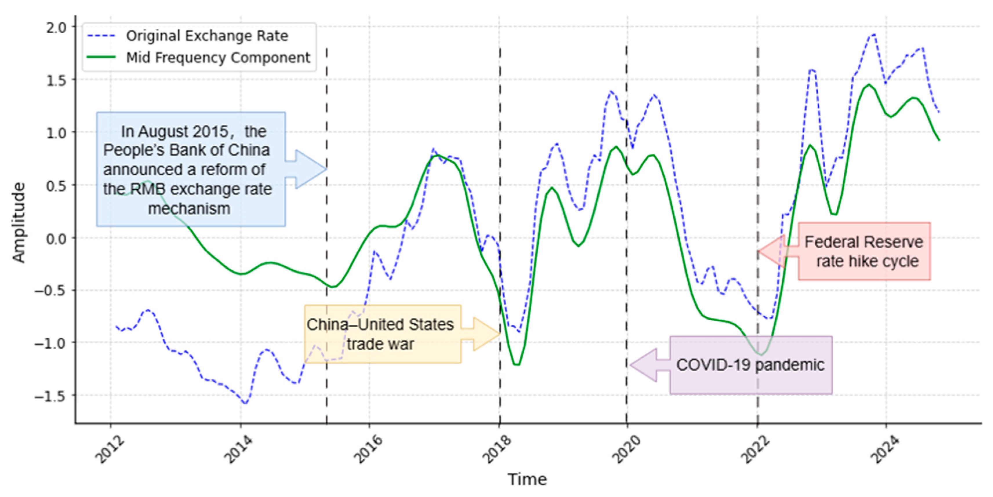
In the medium-frequency domain, the drivers shifted significantly towards policy cycles and event shocks. The Effective Federal Funds Rate (EFFR) emerged as the dominant factor, exerting a far greater influence than money supply metrics. Our results show that high EFFR values—indicative of tightening U.S. monetary policy—exert significant depreciation pressure on the RMB. This frequency band captures the medium-term trends where the effects of central bank policies gradually materialize and structural breaks occur. As illustrated by our event analysis, sharp adjustments in this component correspond closely with major shocks such as the US–China trade frictions and the Federal Reserve’s aggressive interest rate hiking cycle starting in 2022 (Ma et al., 2024 [2]).

In the low-frequency domain, the exchange rate was anchored by macroeconomic fundamentals and strategic assets. We identified the money supply ratio between China and the U.S. (M2) and gold futures prices (COMEX) as the decisive factors. A relative increase in China’s M2 supply was shown to exert long-term depreciation pressure, consistent with monetary theories of exchange rate determination. Furthermore, the strong link with gold prices reflects the complex interplay between global risk hedging and the intrinsic value of the currency (Li, 2024 [3]). This long-run component filters out short-term noise and policy shocks, revealing the secular trends determined by relative economic strength and monetary sovereignty.

Accordingly, this paper makes two contributions. First, we provide horizon-specific evidence on the determinants of USD/CNY by decomposing exchange-rate movements into economically meaningful frequency components and quantifying the relative importance of key drivers within each component. Second, we propose a transparent “decompose-reconstruct-predict-explain” workflow that integrates multi-scale decomposition with interpretable machine learning, thereby linking predictive modeling to economically interpretable insights. Importantly, our primary objective is to complement accurate forecasting with transparent interpretation, rather than pursuing accuracy gains alone; SHAP-based attribution provides transparent, model-based evidence on the sources of exchange rate fluctuations across horizons.

The remainder of the paper is organized as follows. Section 2 reviews the related literature, Section 3 discusses the data sources and indicator selection, Section 4 introduces the methods used in this paper for explainable AI and multi-scale analysis of exchange rates, Section 5 presents the empirical analysis results, and Section 6 concludes the paper.

2. Literature Review

The foreign exchange market is a typical complex system characterized by high volatility and non-stationarity, which inhibits the ability of models to explain its fluctuations and predict its trends. Traditional Empirical Mode Decomposition (EMD) and Ensemble Empirical Mode Decomposition (EEMD) methods have limitations when processing complex signals from the foreign exchange market. For instance, Lin et al. (2012) [4] applied EMD to decompose exchange rates and found that the decomposed subcomponents exhibited mixing frequencies, making it difficult for the model to identify the underlying patterns. To address this issue, Wu and Huang (2009) [5] proposed the EEMD method, which adds Gaussian white noise to the original sequence and processes the newly generated signal multiple times using the EMD algorithm. Yeh et al. (2010) [6] further introduced the Complete Ensemble Empirical Mode Decomposition (CEEMD) method, optimizing the decomposition process by adding two opposite white noise components. These methods help reduce noise interference to some extent, but white noise may still remain within the Intrinsic Mode Functions (IMFs). To solve this problem, Torres et al. (2011) [7] proposed the Complete Ensemble Empirical Mode Decomposition with Adaptive Noise (CEEMDAN). This method does not directly add Gaussian white noise to the original signal, but instead adds IMF components with auxiliary noise after the EMD decomposition. Compared to EEMD and CEEMD, CEEMDAN effectively addresses the issue of white noise transfer from high-frequency to low-frequency components. Therefore, in this paper, we used the CEEMDAN method to decompose exchange rates, improving the decomposition accuracy, which in turn enhanced the reliability and scientific validity of subsequent analyses.

Our study aims to establish a scientific framework to explain the factors influencing exchange rates at different frequencies. Numerous studies have examined the factors affecting exchange rates from various perspectives, including inflation and foreign reserves (Grebenkina & Khandruev, 2021 [8], Korap, 2024 [9], Panopoulou & Souropanis, 2019 [10], Draz et al., 2019 [11]), international variables like oil prices and global interest rates (Breen & Hu, 2021 [12], Zhang & Qin, 2022 [13], Jammazi et al., 2015 [14], Vancsura et al. [15]), market sentiment (Bhargava & Konku, 2023 [16], Wang et al., 2022 [17], Fantazzini, 2025 [18]), and trade dynamics (Bosupeng et al., 2024 [19], Lin & Chen, 2022 [20], Msomi & Muzindutsi, 2025 [21]). Specifically, Ferrara et al. (2021) [22] re-examined the impact of government spending shocks on real exchange rates and inflation in the U.S., finding that increased government spending leads to real exchange rate appreciation and inflationary pressure. Harrison et al. (2024) [23] investigated the long-term effects of global oil market shocks on real effective exchange rates, volatility, and related dynamics. Huynh et al. (2023) [24] analyzed the impact of trade policy uncertainty on the USD exchange rates of the nine most traded currencies in global trade. Aslam et al. (2020) [25] studied the impact of the COVID-19 pandemic on the efficiency of the foreign exchange market. Shahzad et al. (2021) [26] analyzed the dependence between investor sentiment and exchange rate returns. While the existing literature also includes short-term and long-term analyses of factors influencing exchange rates, these studies typically do not systematically decompose exchange rates into components of different frequencies and are often focused on the impact of specific factors on exchange rates in the short- and long-term. Despite the growing body of literature in the field of economics and finance that integrates decomposition methods with machine learning to address diverse issues (Cui et al., 2024 [27], Zu et al., 2024 [28], Han et al., 2025 [29]), the application of this hybrid approach to the study of RMB exchange rate dynamics remains under-explored in the existing research. Therefore, this paper decomposed exchange rates into different frequency components for multi-level differentiation and comparison. We analyzed and compared high, medium, and low-frequency exchange rates from four different perspectives: economic fundamentals, international financial environment, public sentiment, and international trade, systematically revealing the dominant factors at various time scales.

In this paper, we used the SHAP model to study the contribution relationships and structural hierarchy between variables. However, the prerequisite for using the SHAP model is that predictions must first be made, after which the model’s results can be explained and analyzed. Common forecasting methods in the existing literature include Autoregressive Integrated Moving Average (ARIMA), Generalized Autoregressive Conditional Heteroskedasticity (GARCH), and Vector Autoregression (VAR) models (Charfi & Mselmi, 2022 [30]; Zhou et al., 2020 [31]; Escudero et al., 2021 [32]; Liang et al., 2022 [33]). While widely used, these traditional econometric models may not effectively capture the nonlinear relationships and dynamic changes in exchange rates. In contrast, machine learning methods have proven highly effective in addressing these issues for time series forecasting. The seminal work by Gu et al. (2020) [34] demonstrated the value of machine learning in empirical asset pricing, establishing a foundation for its application in capturing complex financial data structures. Building on this, newer applications, such as by Raza and Akhtar (2024) [35], have further validated the predictive power of these techniques in emerging markets. Representative techniques in the current literature include XGBoost, CatBoost, LightGBM, random forests, neural networks, and support vector machines (e.g., Naeem et al., 2021 [36]; Colombo et al., 2020 [37]; Su & Wu, 2023 [38]; Yu et al., 2024 [39]; Neghab et al., 2024 [40], Bilis et al., 2025 [41]). It should be noted that machine learning models are typically “black boxes”, making it difficult to interpret their predictions. The interpretable machine learning model SHAP, proposed by Lundberg and Lee (2017) [42], effectively overcomes this challenge. Therefore, in this study, we used machine learning models to predict exchange rates, compare the performance of XGBoost, CatBoost, LightGBM, and random forests, and selected the best-performing CatBoost model to predict exchange rates. Subsequently, we applied SHAP to analyze the decomposed high, medium, and low-frequency exchange rates.

3. Data Sources and Indicator Selection

This paper selected the monthly midpoint exchange rate data of USD/CNY from January 2012 to September 2024 to represent the fluctuation of the RMB exchange rate. Additionally, the monthly data for 16 selected indicators from four categories—macroeconomic fundamentals, international financial markets, international trade, and public sentiment—were sourced from the National Bureau of Statistics, the People’s Bank of China, the Wind database, and other sources. A summary of the classification of the 16 indicators is shown in Table 1.

Table 1. The summary of variables.

Factor	Indicator	Variable	Abbreviation
Economic Fundamentals	Economic Development Level	Value Added of Industry Enterprises	VAIE
	Inflation Rate	Consumer Price Index	CPI
	Fiscal Policy	Government Fiscal Expenditure	GE
	Monetary Policy	Money Supply	M2
	Foreign Exchange Reserves	Foreign Exchange Reserves	FXR
International Financial Market	International Currency Exchange Rates	US Dollar Index	DXY
	International Market Interest Rates	Effective Federal Funds Rate	EFFR
	International Crude Oil Prices	Brent Crude oil Futures Settlement Price	BFSP
	International Gold Prices	Gold Futures Closing Price	COMEX
International Trade	Terms of Trade	Import Price Index	IPI
		Export Price Index	EPI
	Trade Balance	Balance of Trade	BOT
	Foreign Direct Investment	Foreign Direct Investment	FDI
Public Sentiment	Sentiment Index	Consumer Confidence Index	CCI
		Economic Policy Uncertainty Index	EPU
	Panic Index	S&P 500 Volatility Index	VIX

Note: This table summarizes the 16 explanatory variables used in this study to model USD/CNY exchange rate fluctuations. The dataset covers the period from January 2012 to September 2024 with a monthly frequency. Key specifications include: 1. Value Added of Industry Enterprises (VAIE) serves as a proxy for GDP due to data availability. 2. CPI and M2 are calculated as the ratio of the indices for China and the U.S. to capture relative changes. 3. Data Sources: National Bureau of Statistics, People’s Bank of China, Wind database, and other standard sources. 4. Abbreviations: Most abbreviations follow standard conventions in the literature (M2, FXR, DXY, COMEX EPU, VIX) or are formed from the initials of the corresponding variable names. For variables without widely accepted abbreviations, we adopted concise notations; specifically, GE denotes Government Fiscal Expenditure and BFSP denotes Brent Crude Oil Futures Settlement Price.

In the category of macroeconomic fundamentals, Gross Domestic Product (GDP) is commonly used to measure the level of economic development. However, since GDP data are available only on a quarterly basis, we used China’s Value Added of Industry Enterprises (VAIE) monthly data as a substitute. The inflation rate is represented by the Consumer Price Index (CPI), and monetary policy is represented by the money supply (M2). Given that the exchange rate data selected in this study pertain to USD/CNY, the CPI and M2 were expressed as the ratio of the indices for China and the U.S. In addition, government expenditure (GE) data were selected to represent government fiscal policy, and foreign exchange reserves (FXR) were included.

In the international financial market category, the U.S. dollar, as the world’s primary reserve currency, directly affects the relative value of the RMB. Given the U.S. dollar’s status as the dominant global currency, the U.S. Dollar Index (DXY) was selected as a representative variable. Since this paper focused on the factors influencing the USD/CNY exchange rate, the Effective Federal Funds Rate (EFFR) was chosen to represent U.S. monetary policy. The international crude oil price is represented by the Brent crude oil futures settlement price (BFSP), and the international gold price is represented by the average closing price of gold futures (COMEX).

In the international trade category, the import price index (IPI) and export price index (EPI) were used to represent trade conditions. This section also includes the Balance of Trade (BOT) and foreign direct investment (FDI). In the category of public sentiment, the Consumer Confidence Index (CCI) and the Economic Policy Uncertainty Index (EPU) were selected, while the panic index was represented by the S&P 500 Volatility Index (VIX). Descriptive statistics for these indicators are shown in Table 2. Although the descriptive statistics reveal basic characteristics of the exchange rate data, they cannot capture the complex, nonlinear, and multi-scale features. Therefore, in the next section, we introduce a hybrid framework to decompose and model these complexities.

Table 2. The descriptive statistics of all variables.

	N	Max	Min	Mean	Std. Dev.	Skewness	Kurtosis
EX	153	7.307	6.051	6.618	0.358	0.239	−1.199
CPI	153	24.000	13.758	1.208	3.049	2.613	25.823
M2	153	14.554	8.768	11.664	1.410	0.010	−0.504
FXR	153	39,932.130	29,982.040	32,870.752	2609.926	1.421	0.822
VAIE	153	52.339	−25.867	6.700	6.362	1.706	21.577
GE	153	37,742	6897.340	17,260.864	6370.799	0.798	0.353
EFFR	153	5.330	0.050	1.333	1.744	1.361	0.488
DXY	153	111.937	78.922	94.029	8.183	−0.396	−0.714
BFSP	153	124.545	26.637	75.736	24.205	0.170	−1.041
COMEX	153	2571.741	1069.282	1545.950	331.621	0.698	−0.199
IPI	153	118.000	85.000	101.164	7.925	0.305	−0.499
EPI	153	115.700	90.300	101.520	5.229	0.474	0.185
FDI	153	245.800	65.000	115.758	31.788	1.261	2.110
BOT	153	988.050	−619.920	438.706	257.485	−0.445	1.387
VIX	153	57.737	10.125	17.601	6.131	2.576	11.826
CCI	153	127.000	85.500	107.557	12.606	−0.222	−1.081
EPU	153	970.830	40.403	436.748	255.736	0.298	−1.048

Note: This table reports descriptive statistics for the USD/CNY exchange rate (EX) and the 16 explanatory variables listed in Table 1 using monthly observations from January 2012 to September 2024. N denotes the number of monthly observations. Max, Min, Mean, Std. Dev., Skewness, and Kurtosis are computed on the sample values, respectively.

4. Methodology

4.1. Research Framework

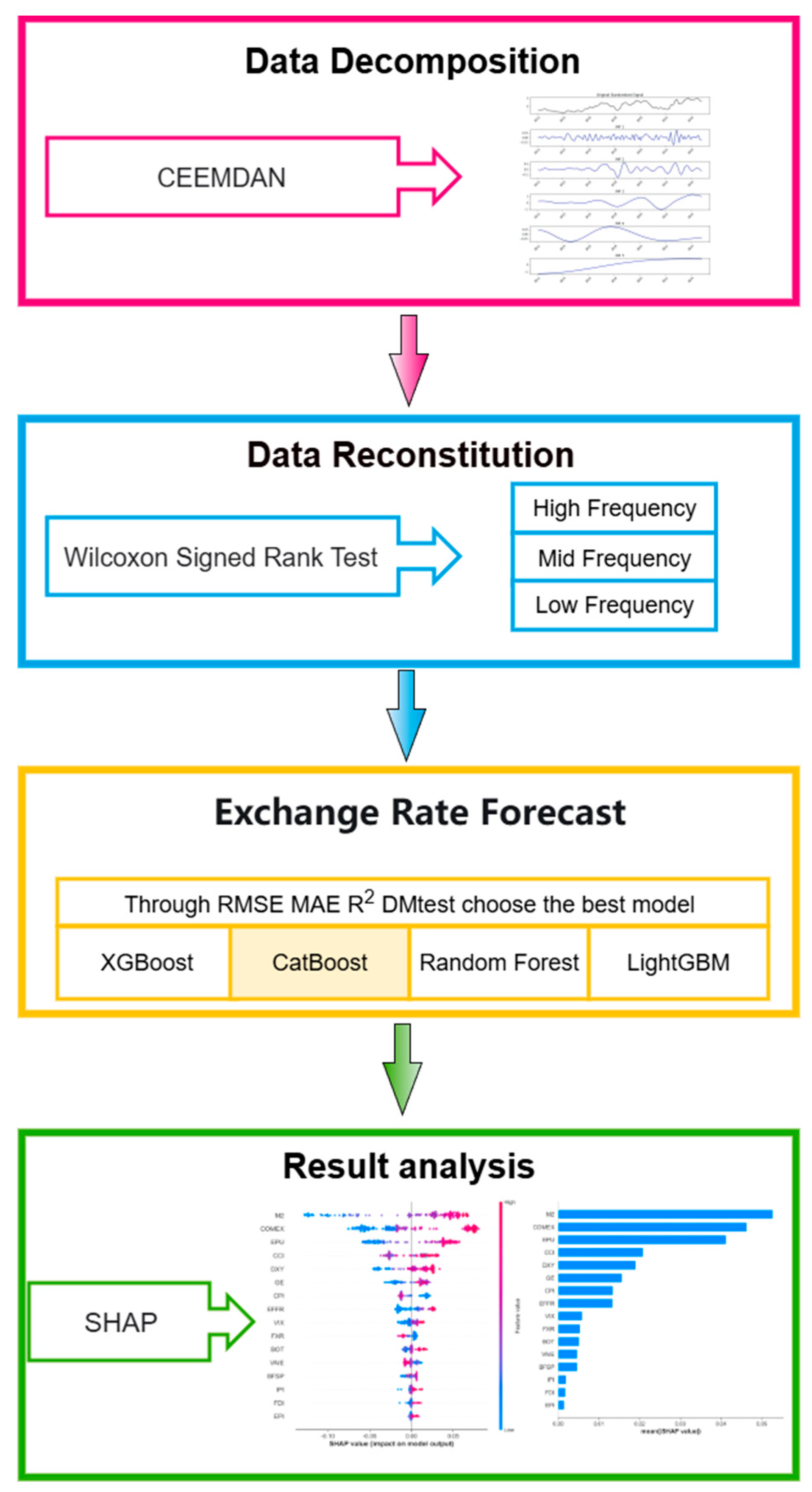
We propose the CEEMDAN-PE-CatBoost-SHAP method, combining multi-scale analysis and explainable AI tools, to study the monthly exchange rate data of USD/CNY from January 2012 to September 2024. As shown in Figure 1, our research process follows four steps: decomposition, reconstruction, prediction, and analysis.

Figure 1. The research framework.

Step 1: The CEEMDAN method is applied to decompose the exchange rate data into four IMFs from high to low frequency plus one residual.

Step 2: The Welch Power Spectral Density estimate and Permutation Entropy are used to characterize the spectral features and complexity of the series, respectively. Based on these metrics, the decomposed exchange rate data are reconstructed into high-, medium-, and low-frequency bands.

Step 3: Based on historical literature, 16 indicators from four key factors influencing exchange rates—economic fundamentals, international financial environment, public sentiment, and international trade—are selected. These indicators are used to predict the exchange rate series sequentially using Random Forest, XGBoost, CatBoost, and LightGBM models. To ensure the robustness of model selection, we employed the Diebold–Mariano (DM) test to statistically compare the predictive accuracy of these models. The DM test results consistently identified CatBoost as the superior model across different frequency bands.

Step 4: The SHAP model is employed to explore the extent to which these 16 indicators influence the exchange rate at different frequencies. The analysis of high, medium, and low-frequency exchange rates is conducted using composite charts, SHAP summary plots, and importance ranking charts.

4.2. Multi-Scale Decomposition

4.2.1. CEEMDAN

CEEMDAN, an advanced signal decomposition technique introduced by Torres et al. (2011) [7], offers a robust solution for analyzing nonlinear and non-stationary time series. By integrating adaptive noise into the decomposition process, CEEMDAN effectively mitigates the commonly observed issue of mode mixing in traditional Empirical Mode Decomposition (EMD). This method builds upon the foundations laid by Ensemble Empirical Mode Decomposition (EEMD) and its complementary variant (CEEMD), refining the process by adaptively adjusting the magnitude of added noise at each iteration. This results in a more accurate extraction of Intrinsic Mode Functions (IMFs) from complex signals. We selected CEEMDAN over strictly EMD or EEMD because it effectively addresses the ‘mode mixing’ problem and provides a negligible reconstruction error, which is crucial for the precision of financial time series forecasting.

Generate modified signal x_i(t) by superimposing Gaussian white noise n(t) to the source signal x(t):

$$x_i\left(t\right)=x\left(t\right)+n_i\left(t\right)$$

(1)

Apply EMD to each x_i(t), then derive the first IMF component through ensemble averaging, then extract the primary residual:

$${\mathrm{I}\mathrm{M}\mathrm{F}}_1\left(t\right)={\displaystyle \frac{\sum _{i=1}^m{\mathrm{I}\mathrm{M}\mathrm{F}}_{i1}^1\left(t\right)}{m}}$$

(2)

$$r_1\left(t\right)=x\left(t\right)-{\mathrm{I}\mathrm{M}\mathrm{F}}_1\left(t\right)$$

(3)

Inject noise into r_i(t) before EMD to derive ${\mathrm{I}\mathrm{M}\mathrm{F}}_{\mathrm{i}+1}\left(\mathrm{t}\right)$ until monotonic residuals emerge:

$$X\left(t\right)=\sum _{i=1}^n{\mathrm{I}\mathrm{M}\mathrm{F}}_i\left(t\right)+r_n\left(t\right)$$

(4)

To balance computational efficiency and decomposition stability, the number of ensembles is set to 200, and the standard deviation of the added white noise is set to 0.4.

4.2.2. Permutation Entropy (PE)

Permutation Entropy (PE), introduced by Bandt and Pompe (2002) [43], serves as a robust and computationally efficient measure for assessing the complexity of time series data. Particularly effective for analyzing systems characterized by nonlinearity and nonstationarity, PE is noted for its resilience to noise and minimal computational overhead.

For a time series x(i), construct embedding matrix with dimension m and delay t:

$$\mathrm{X} = \begin{array}{cccc}x\left(1\right)& x\left(1+t\right)& \dots & x\left(1+\left(m-1\right)t\right)\\ ⋮& ⋮& & ⋮\\ x\left(j\right)& x\left(j+t\right)& \dots & x\left(j+\left(m-1\right)t\right)\\ ⋮& ⋮& & ⋮\\ x\left(G\right)& x\left(G+t\right)& \dots & x\left(G+\left(m-1\right)t\right)\end{array}$$

(5)

where G = N − (m − 1)t denotes the reconstructed vector count.

For each vector X_j, rank components in ascending order:

$$x(i+(j_1-1\left)t\right)\le x(i+(j_2-1\left)t\right)\le \cdots \le x(i+(j_m-1\left)t\right)$$

(6)

Each such permutation corresponds to one of the m! possible symbol sequences. By calculating the relative frequency $P_l$, the entropy is defined fusing the Shannon entropy formula:

$$PE\left(m\right)=-\sum _{l=1}^{m!}{P}_{l}ln{P}_l$$

(7)

The maximum entropy is $\ln \left(m!\right)$, which occurs when all permutations are equally probable. Normalizing by this value yields:

$$PE={\displaystyle \frac{PE\left(m\right)}{\ln \left(m!\right)}}$$

(8)

where the PE range is 0 ≤ PE ≤ 1. A higher PE indicates greater dynamical complexity within the time series.

4.3. Interpretable AI Analysis

The technical rationale for integrating these specific components is threefold. First, while CEEMDAN effectively handles the non-stationarity of exchange rates, the resulting IMFs often contain redundant noise or fragmented information. By introducing PE as a reconstruction criterion, we bridge the gap between signal processing and economic intuition, ensuring that the input features for the machine learning stage are aligned with distinct market frequencies. CatBoost was chosen as the primary forecasting engine; theoretically, its ordered boosting mechanism is designed to combat prediction shift and gradient bias, which often plague financial time series with complex temporal dependencies. This aligns with our empirical findings where CatBoost consistently outperformed other ensemble methods in terms of predictive accuracy. Finally, the integration of SHAP transforms the CatBoost model from a black-box into a structural analysis tool. Unlike traditional importance metrics that only rank features, our SHAP-based approach quantifies the marginal contribution of each economic driver in original units, providing a rigorous, game-theoretic basis for comparing drivers across different time horizons. This integrated pipeline ensures that our findings are both statistically robust and economically interpretable. A comprehensive exposition of the mathematical principles and operational procedures for each component of this framework is provided in the following subsections.

4.3.1. Random Forest

The Random Forest method, developed by Breiman (2001) [44], is a robust ensemble learning method that aggregates predictions from multiple decision trees. For regression tasks, it outputs the mean of the predictions from all individual trees, thereby enhancing predictive accuracy while mitigating overfitting. Each tree in the forest is trained on a bootstrap sample of the data and considers a randomly selected subset of features at every split. The overall prediction for an input vector x is given by aggregating the outputs of all base learners $h_i\left(X\right)$:

$$\widehat{Y}={\displaystyle \frac{1}{N}}\sum _{i=1}^N{h}_i\left(X\right)$$

(9)

4.3.2. XGBoost

Extreme Gradient Boosting (XGBoost), introduced by Chen and Guestrin (2016) [45], is a high-performance implementation of gradient boosting that emphasizes computational efficiency and scalability. It builds additive tree models in a sequential manner, where each subsequent tree is trained to predict the residuals of the previous ensemble. To avoid overfitting, a pruning strategy is employed, removing tree nodes with low contributions. The update rule for predictions is:

$${\widehat{y}}_i^{\left(t\right)}=\sum _{k=1}^t{f}_k\left(x_i\right)={\widehat{y}}_i^{\left(t-1\right)}+f_t\left(x_i\right)$$

(10)

Here, f_t denotes the newly added regression tree at iteration t, and x_i represents the input features of the i-th instance.

4.3.3. LIGHTGBM

Light Gradient Boosting Machine (LIGHTGBM), developed by Ke et al. (2017) [46], is a gradient boosting framework that excels in handling large-scale and high-dimensional data. It employs leaf-wise tree growth, allowing for faster convergence and improved accuracy compared to level-wise methods. LightGBM is optimized for speed and memory efficiency, supporting both parallel and GPU learning. The model can be expressed as:

$$\widehat{Y}=\sum _{t=1}^T{f}_t\left(X\right)$$

(11)

Here, f_t(x) denotes the regression tree at iteration t, and T is the total number of trees.

4.3.4. CatBoost

Categorical Boosting (CatBoost), proposed by Prokhorenkova et al. (2018) [47], is a gradient boosting framework tailored for datasets containing categorical variables. It introduces two key innovations: a novel method for encoding categorical data and a permutation-driven ordered boosting scheme that reduces prediction bias. Compared to XGBoost and LightGBM, CatBoost handles categorical features more naturally and is less prone to overfitting due to its ordered boosting mechanism, making it suitable for our financial time series. The predictive function is defined as:

$$\widehat{Y}=\sum _{t=1}^T{h}_t\left(X\right)$$

(12)

Here, ℎ(X) captures the decision function at iteration t, and the model learns the conditional distribution f_t (X_k, Y_k) over the training data.

4.3.5. Evaluation Metrics

The predictive accuracy of machine learning models is assessed using the following statistical metrics:

$$MAE={\displaystyle \frac{1}{N}}{\sum }_{i=1}^N\left({\widehat{Y}}_i-Y_i\right)$$

(13)

$$MSE={\displaystyle \frac{1}{N}}\sum _{i=1}^N{\left({\widehat{Y}}_i-Y_i\right)}^2$$

(14)

$$RMSE=\sqrt{{\displaystyle \frac{1}{N}}\sum _{i=1}^N{\left({\widehat{Y}}_i-Y_i\right)}^2}$$

(15)

$$R^2={\displaystyle \frac{\sum _{i=1}^N{\left({\widehat{Y}}_i-{\overline{Y}}_i\right)}^2}{\sum _{i=1}^N{\left(Y_i-{\overline{Y}}_i\right)}^2}}$$

(16)

4.3.6. SHAP

Although machine learning models are powerful tools for time series forecasting, their interpretability remains a major challenge. To address this, Lundberg and Lee (2017) [42] proposed the SHAP framework, which leverages Shapley values from cooperative game theory to explain individual predictions. SHAP estimates the contribution of each input feature to the model’s output by evaluating marginal contributions across all possible feature permutations. The SHAP value for a feature subset z’ is computed as:

$${\varnothing }_i\left(f,x\right)=\sum _{z^{\prime }⊑x^{\prime }}{\displaystyle \frac{\left|z^{\prime }\right|!\left(M-\left|z^{\prime }\right|-1\right)!}{M!}}\left[f_x\left(z^{\prime }\right)-f_x\left(z^{\prime \backslash }i\right)\right]$$

(17)

Here, M is the total number of features, and f_x (z′) is the model prediction using the subset of features.

To quantify the global importance of each variable, we calculated the Mean Absolute SHAP Value. This metric represents the average impact of a feature on the magnitude of the model output across all observations:

$${\mathrm{I}}_{\mathrm{j}}={\displaystyle \frac{1}{\mathrm{N}}}{\sum }_{\mathrm{i}=1}^{\mathrm{N}}\left|{\mathsf{\varphi }}_{\mathrm{j}}^{\left(\mathrm{i}\right)}\right|$$

(18)

where $N$ is the total number of samples and ${\mathrm{\varnothing }}_{\mathrm{j}}^{\left(\mathrm{i}\right)}$ is the SHAP value of feature for the observation. A higher value indicates that the feature has a stronger overall influence on the exchange rate forecasting.

4.4. Model Training and Hyperparameter Selection

The machine learning models employed in this study were trained using an expanding-window forecasting scheme with time-order preservation of the datasets. The first 70% of the chronologically sorted observations served as the initial training window, followed by recursive one-step-ahead forecasting on the remaining observations.

All models underwent systematic hyperparameter tuning using grid search combined with time-series cross-validation. The optimization criterion was Mean Absolute Error (MAE), selected for its robustness to outliers and interpretability in the context of exchange rate forecasting. The best hyperparameters for each model are specified below:

(1) Random Forest: n_estimators = 1200, max_depth = 7, min_samples_leaf = 1.

(2) CatBoost: iterations = 800, depth = 4, learning rate = 0.05.

(3) XGBoost: n_estimators = 800, max_depth = 3, learning rate = 0.05.

(4) LightGBM: n_estimators = 800, learning rate = 0.05, max_depth = 4.

5. Empirical Study

5.1. Multi-Scale Decomposition

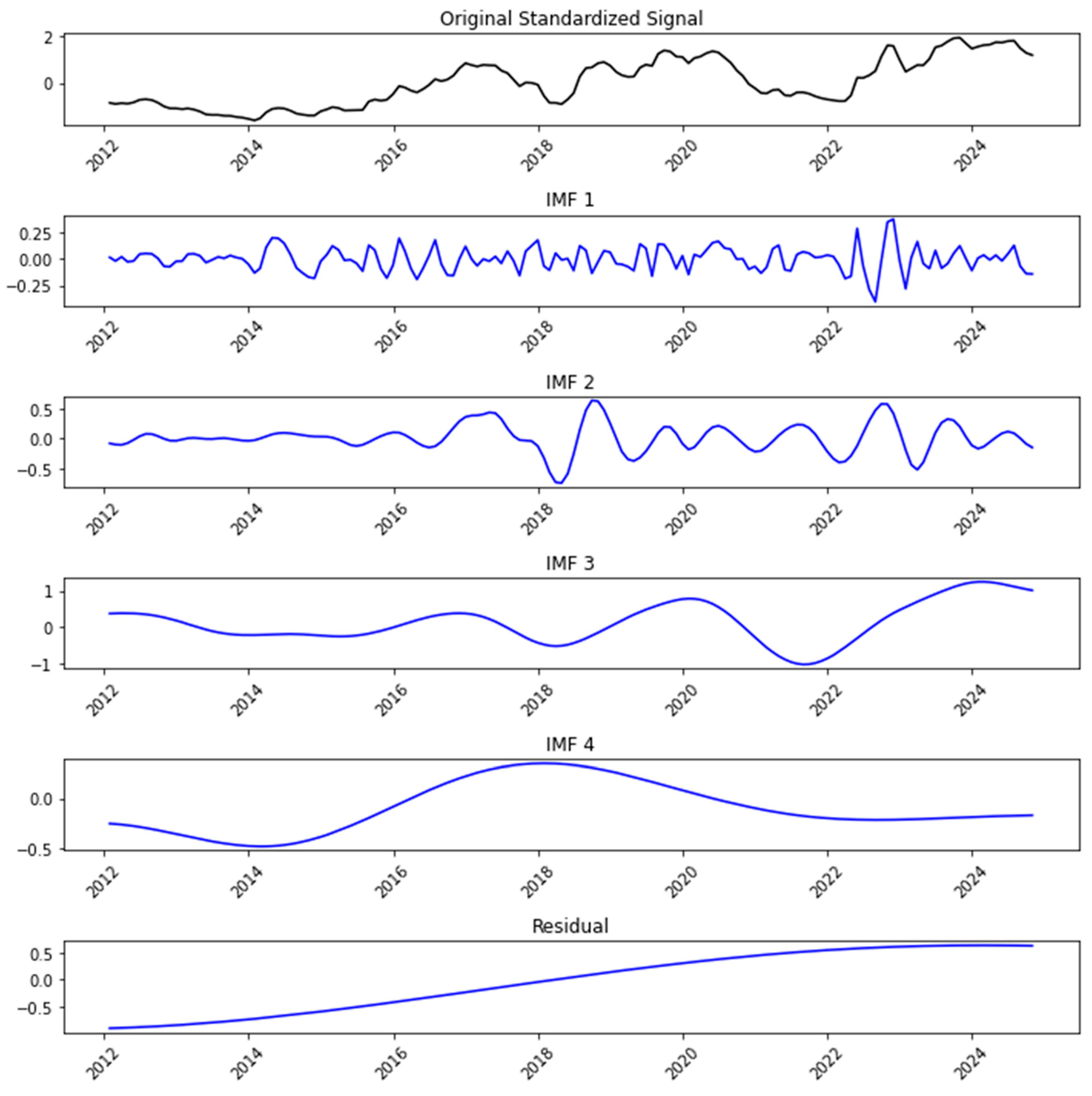
First, the CEEMDAN method was used to decompose the monthly exchange rate into four IMFs from high to low frequency plus one residual, as shown in Figure 2. To characterize their time scales, we calculated the dominant periods of each IMF using the Welch power spectral density estimate. Specifically, IMF1 (peak period: 5.7 months) exhibited significant high-frequency fluctuations, characterized by rapid oscillation and relatively small amplitude. IMF2 (20.1 months) and IMF3 (38.5 months) displayed similar fluctuation characteristics in terms of amplitude and periodic variation. Compared to IMF1, the fluctuation frequencies of IMF2 and IMF3 were notably lower with longer periods, manifesting as medium-frequency oscillations. Finally, IMF4 and the residual exhibited distinct low-frequency characteristics, with periods exceeding 77 months.

Figure 2. The CEEMDAN decomposition results. Note: The original monthly exchange rate series was decomposed into four IMFs and a residual term.

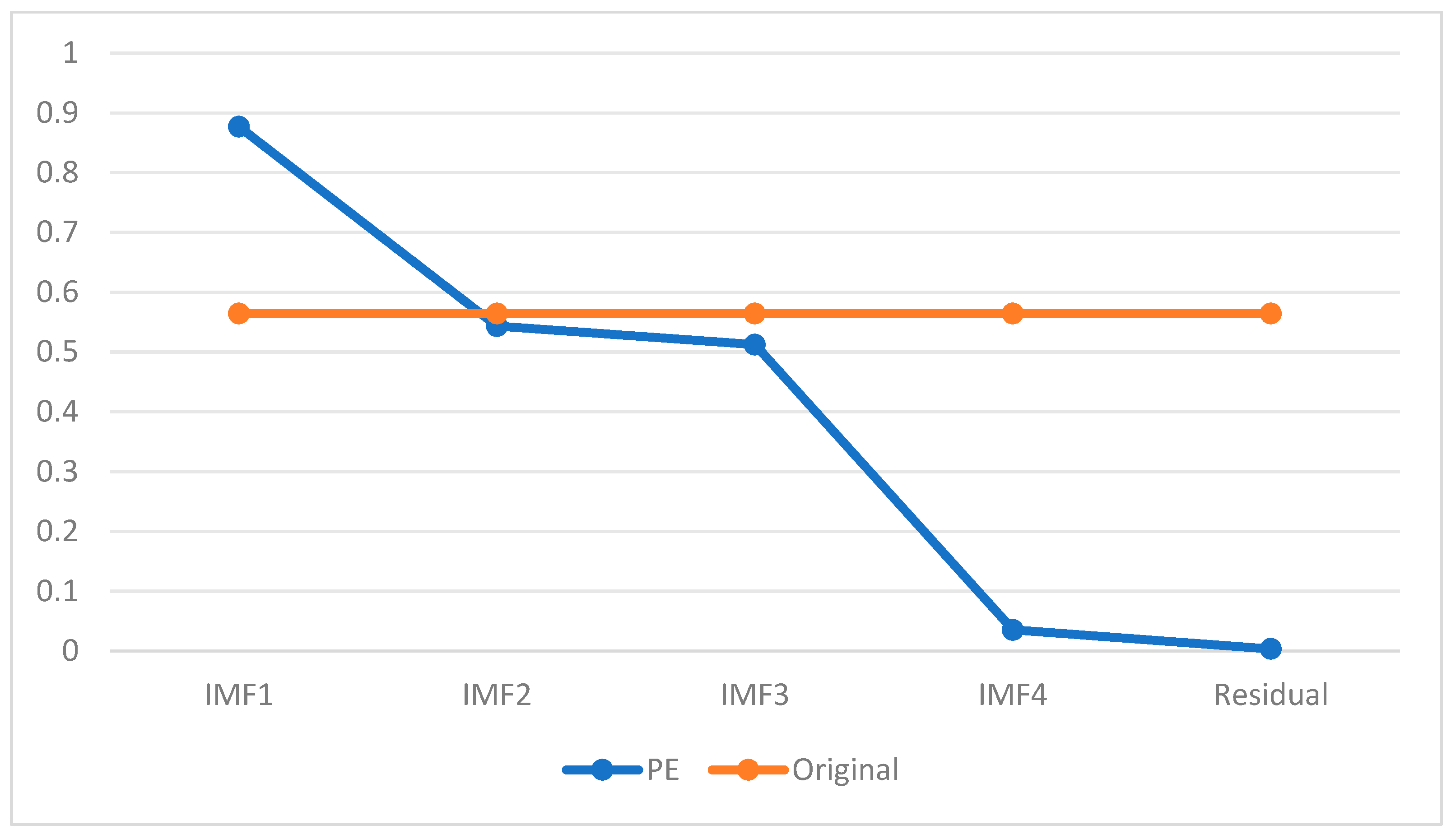
Next, PE was used to assess the complexity of the five IMFs. A larger PE value indicates a higher degree of complexity in the sequence. We plotted the PE values of the original sequence in Figure 3 to identify which subsequences were closer to each other, followed by their classification and reconstruction. The IMFs were divided into three categories based on their PE values in comparison to the original sequence: those with PE values close to, smaller than, or larger than the PE value of the original sequence (Zhang et al., 2014) [48]. As shown in Figure 3, the PE values of IMF2 and IMF3 were close to those of the original sequence, the PE value of IMF1 was significantly higher than that of the original sequence, and the PE values of IMF4 and the residual were noticeably lower.

Figure 3. PE value of five IMFs. Note: Permutation Entropy (PE) characterizes the complexity and irregularity of a time series, where a higher PE value indicates greater complexity. The orange line represents the PE value of the original USD/CNY exchange rate series (EX). The blue line plots the PE values of the components obtained via CEEMDAN decomposition (IMF1–IMF4 and the Residual).

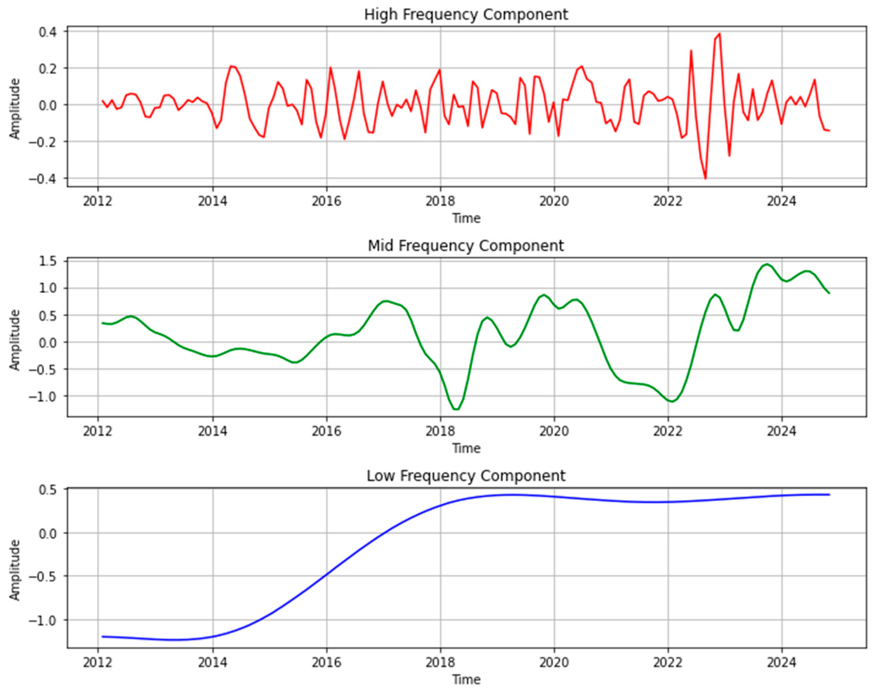
In conclusion, we adopted a reconstruction strategy primarily driven by PE values and corroborated by the time-scale analysis from PSD. IMF1 was classified as a high-frequency component, IMF2 and IMF3 were combined into a medium-frequency component, and IMF4 and the residual were grouped into a low-frequency component. The signal graphs of the high, medium, and low-frequency components are shown in Figure 4. Table 3 reports the statistical metrics of these frequency components.

Figure 4. The three components for exchange rate. Note: Frequency bands are formed according to the components’ complexity and frequency characteristics. High-frequency was reconstructed from IMF1; Mid-frequency from IMF2 and IMF3; Low-frequency from IMF4 and the Residual, based on Permutation Entropy values.

Table 3. The descriptive statistics of different frequencies.

	N	Max	Min	Mean	Var	Skewness	Kurtosis
High_Frequency	153	0.298	−0.343	0.001	0.019	−0.131	−0.078
Mid_Frequency	153	0.346	−0.248	−0.002	0.022	0.248	−0.698
Low_Frequency	153	6.923	6.283	6.618	0.049	−0.154	−1.439

Note: This table reports descriptive statistics for the reconstructed high-, mid-, and low-frequency components. N denotes the number of monthly observations. Max, Min, Mean, Var, Skewness and Kurtosis were computed on the reconstructed high-, mid-, and low-frequency components, respectively.

5.2. Interpretable AI Analysis

To ensure robust results, we adopted an expanding window approach to preserve temporal dependencies in our time series data. The first 70% of the chronologically sorted observations served as the initial training window, followed by recursive one-step-ahead forecasting on the remaining observations. We implemented and compared four machine learning models: Random Forest, XGBoost, LightGBM, and CatBoost.

The predictive performance was assessed using MAE, RMSE, and R². Furthermore, the Diebold–Mariano (DM) test was employed to determine whether the differences in forecast accuracy between the best-performing model and the alternatives were statistically significant. As summarized in Table 4, CatBoost achieved the highest predictive accuracy with an R² of 0.8539, outperforming the other models. Crucially, the DM test statistics and corresponding p-values (p < 0.05) confirmed that the predictive superiority of CatBoost over Random Forest, XGBoost, and LightGBM was statistically significant.

Table 4. Machine learning model performance and DM test results.

	MAE	RMSE		R2
Random Forest	0.1427	0.1783		0.7339
XGboost	0.1206	0.1621		0.7801
CatBoost	0.0999	0.1296		0.8539
LightGBM	0.1182	0.1629		0.7776
	DM_stat		p_value
CatBoost vs. XGBoost	−2.3437		0.0118 *
CatBoost vs. LightGBM	−2.3331		0.0121 **
CatBoost vs. RandomForest	−3.9108		0.0001 ***

Note: 1. ***, ** and * denote significance at 1%, 5%, 10%, respectively. 2. The null hypothesis of the DM test assumes equal predictive accuracy between the two compared models. A negative DM statistic indicates that the first model (CatBoost) has a lower forecast error than the second.

Given its superior performance, the CatBoost model was subsequently integrated with SHAP to conduct an interpretable AI analysis. While machine learning models are often viewed as black boxes, SHAP allows us to quantify the contribution of each feature to the model’s output, thereby identifying the key drivers of exchange rate fluctuations.

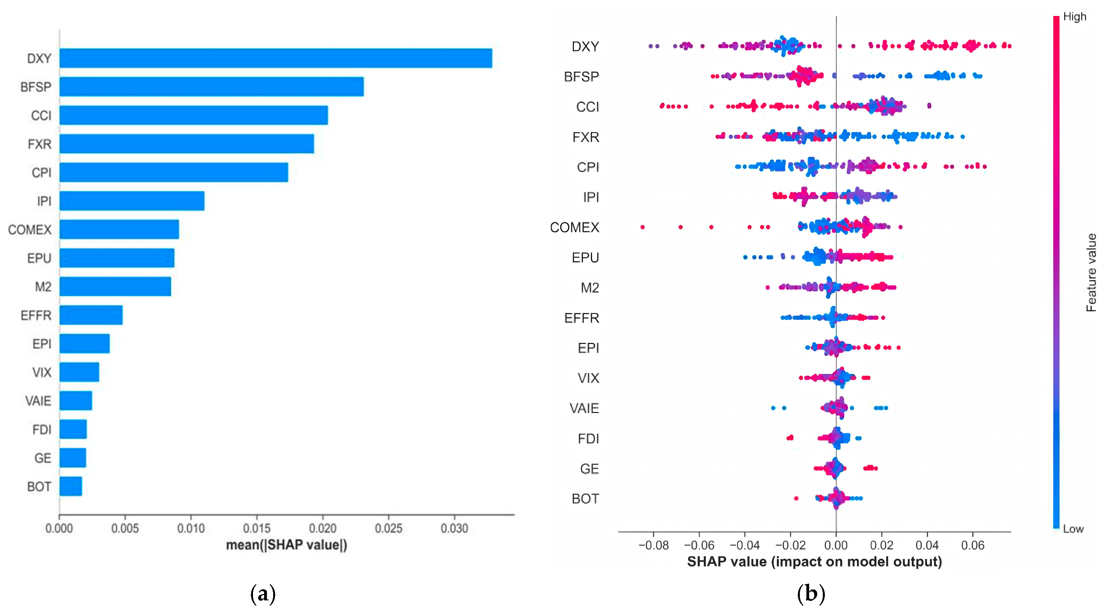
Before analyzing specific frequency bands, we clarified the interpretation of the SHAP plots. The Variable Importance Bar Charts rank features based on their average absolute impact. The SHAP Summary Plots provide a detailed view of the direction of influence: each point represents an observation; the color indicates the feature value (red for high, blue for low), and its position on the horizontal axis indicates whether it drives the USD/CNY exchange rate up (positive SHAP, depreciation) or down (negative SHAP, appreciation).

5.2.1. High-Frequency

Figure 5a,b presents the importance ranking of 16 variables for high-frequency exchange rates and the SHAP summary plot, respectively. As shown, the U.S. Dollar Index (DXY), which represents international currency exchange rates, is the most critical feature in the model, aligning with the dominant role of the U.S. Dollar Index in global foreign exchange markets. Following that, international crude oil prices, represented by the Brent Crude Oil Futures Settlement Price (BFSP), and public sentiment factors such as the Consumer Confidence Index (CCI) play significant roles. These indicators have a large average impact on the model output, indicating their strong explanatory power in exchange rate fluctuations.

Figure 5. Contribution of input variables to High-Frequency exchange rate: (a) Global variable importance based on mean absolute SHAP values; (b) SHAP summary plot illustrating the distribution of feature impacts.

Figure 5b primarily illustrates how different variable values influence the direction of the model’s output. Specifically, when DXY is high (red dots), it positively drives the USD/CNY exchange rate (indicating RMB depreciation), whereas lower DXY values (blue dots) negatively impact the exchange rate. This aligns with the general economic principle that when the U.S. Dollar Index rises, other currencies depreciate against the dollar, leading to an increase in the USD appreciating against other currencies. The Consumer Confidence Index (CCI) showed a concentration of red dots in the negative SHAP value region, suggesting that an increase in consumer confidence pushes the RMB to appreciate. This is mainly because the CCI reflects the domestic economic outlook, which encourages capital inflows and increased consumer spending, thereby enhancing the potential for RMB appreciation. This finding is consistent with Kumari et al. (2022) [1], who explored the relationship between sentiment indicators, such as the CCI, and the U.S. dollar exchange rate, concluding that optimism in sentiment indices leads to short-term USD appreciation.

The higher values of Brent crude oil futures settlement price (BFSP) (red dots) were concentrated in the region with negative SHAP values, indicating that an increase in BFSP leads to a decrease in the USD/CNY exchange rate, and thus an appreciation of the RMB against the USD. This view is supported by Liu et al. (2021) [49], who studied the relationship between oil prices and exchange rates in seven oil-importing and seven oil-exporting countries. Their findings show that when oil prices rise (or fall), foreign currencies appreciate (or depreciate) against the USD.

In conclusion, we consider monthly trading activities and public sentiment as key factors driving high-frequency exchange rate fluctuations. Since market participants’ trading behaviors and sentiment changes are influenced by various factors such as international financial markets, policy shifts, and geopolitical events, these impacts are quickly reflected in the market and significantly affect the exchange rate trends in the short-term.

5.2.2. Mid-Frequency

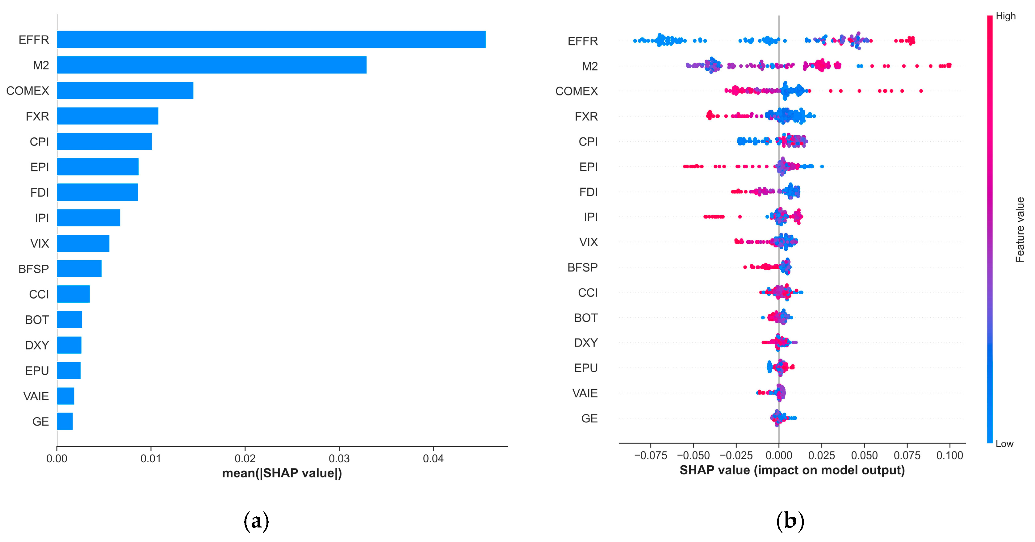
Figure 6a,b illustrates the importance ranking of variables for the mid-frequency exchange rate and the SHAP summary plot, respectively. From Figure 6a, it can be observed that the variables with a significant impact on the model output are the Effective Federal Funds Rate (EFFR), which represents the U.S. Federal Reserve’s monetary policy, and the ratio of money supply between China and the U.S. (M2), with EFFR exerting a far greater influence on the mid-frequency exchange rate than M2. Figure 6b shows that when EFFR is at a high value (indicated by the red color), the SHAP value is significantly positive, suggesting that an interest rate hike by the Federal Reserve puts pressure on the RMB to depreciate. This view is supported by Ma, Z. et al. (2024) [2], whose research used the EFFR as a key indicator to measure the tightening of U.S. monetary policy. Their findings indicate that tightening U.S. monetary policy leads to the depreciation of real exchange rates in other countries, which aligns with the logic that the Fed’s tightening policy strengthens the U.S. dollar. Specifically, the increase in U.S. interest rates attracts capital back to the U.S., causing a relative depreciation of the RMB.

Figure 6. Contribution of input variables to Mid-Frequency exchange rate: (a) Global variable importance based on mean absolute SHAP values; (b) SHAP summary plot illustrating the distribution of feature impacts.

Generally speaking, medium-frequency exchange rate fluctuations reflect the medium- to long-term trends in the economy and policy. For example, the effects of government or central bank monetary policies take time to manifest, and the persistent impact of event shocks gradually influences exchange rate movements. Figure 7 visually aligns specific macroeconomic shocks with the extracted medium-frequency component. Instead of random noise, the fluctuations capture the persistent impact of structural breaks and policy shifts. Notably, the sharp adjustments correspond to the 2015 RMB exchange rate mechanism reform, the escalation of U.S.–China trade frictions (2018), and the global monetary policy divergence following the COVID-19 pandemic. In particular, the sustained upward trend starting in 2022 reflects the aggressive interest rate hikes by the Federal Reserve, confirming that medium-term exchange rate dynamics are largely driven by policy cycles and event shocks. In conclusion, as the effects of policies gradually materialize and the impact of event shocks continues to unfold, market expectations and risk preferences adjust, driving noticeable fluctuations in exchange rates in the medium-term. These fluctuations reflect the market’s gradual response to macroeconomic conditions and policy changes, making the medium-frequency exchange rate an important indicator for observing the effects of economic policies and the impact of major events.

Figure 7. Impact of major events on the Mid-Frequency exchange rate.

5.2.3. Low-Frequency

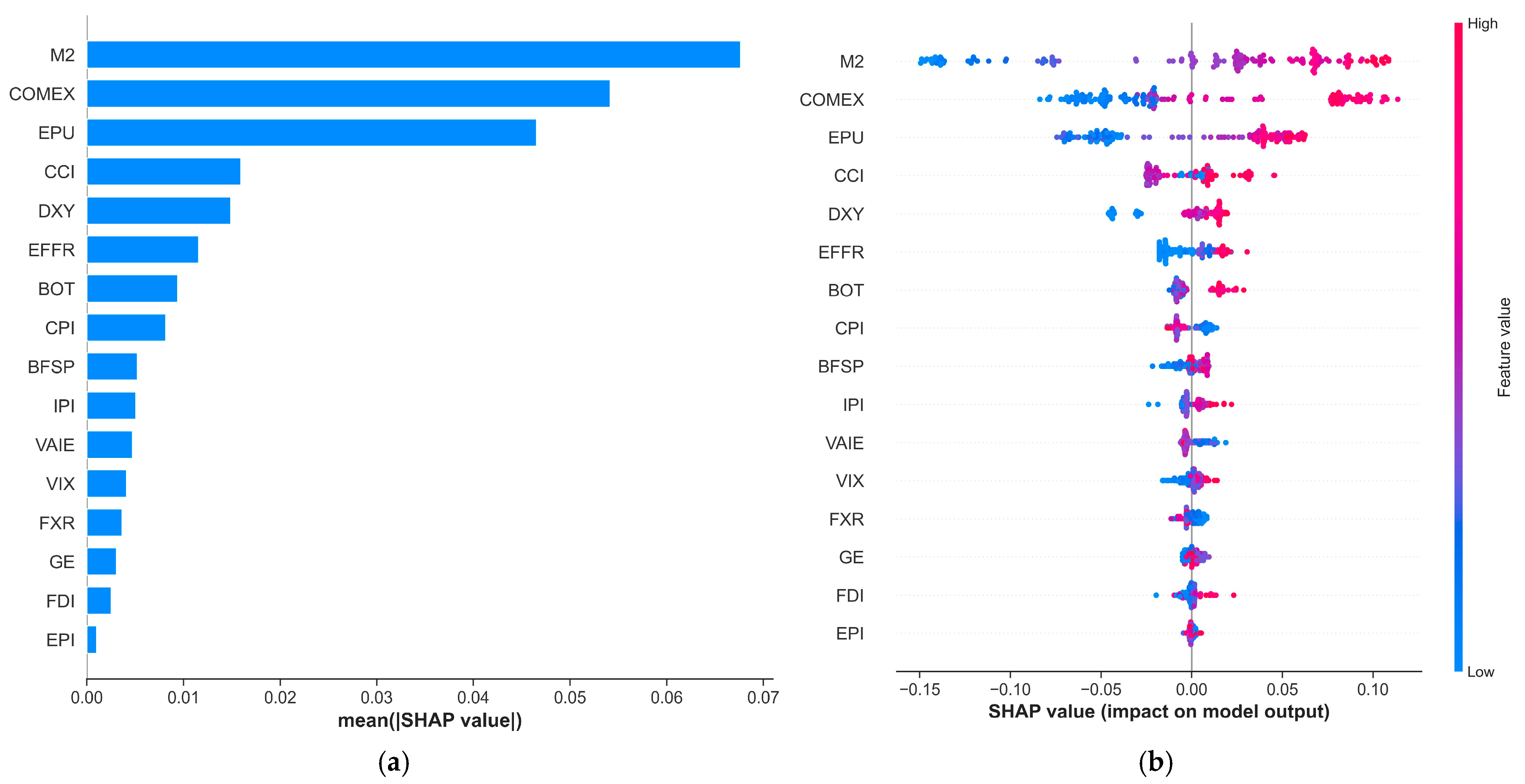
Figure 8a,b presents the importance ranking of 16 variables for low-frequency exchange rates and the SHAP summary plot, respectively. As shown in Figure 8a, the money supply ratio (M2) and gold futures prices (COMEX) were the dominant factors in the long run. Economic Policy Uncertainty (EPU) also showed a high importance score, indicating that long-term exchange rate trends are primarily anchored by monetary fundamentals and global risk hedges. Figure 8b reveals the underlying logic. For M2, red dots (high values) were concentrated in the positive SHAP region, suggesting that a relative increase in China’s money supply compared to the U.S. exerts long-term depreciation pressure on the RMB. For COMEX, high values (red) were also associated with positive SHAP values. This aligns with the view of Li (2024) [3], where rising commodity and gold prices may signal increased import costs or global dollar strength, leading to RMB depreciation in the low-frequency component.

Figure 8. Contribution of input variables to Low-Frequency exchange rate: (a) Global variable importance based on mean absolute SHAP values; (b) SHAP summary plot illustrating the distribution of feature impacts.

Generally speaking, the relationship between gold prices and the RMB exchange rate is often quite complex. First, as a safe-haven asset, gold prices are closely linked to global market risk sentiment. In the event of geopolitical conflicts, financial crises, or other risk events, investors tend to purchase gold as a hedge, thereby driving up its price. Gold prices are also closely tied to monetary policy. Specifically, accommodative policies from the Federal Reserve tend to increase gold prices while weakening the U.S. dollar, indirectly leading to a depreciation of the USD/CNY exchange rate. Conversely, when tightening policies from the Federal Reserve cause the U.S. dollar to strengthen, the USD/CNY exchange rate appreciates, and gold prices may decline. The relative changes in U.S. and Chinese monetary policies are among the core factors affecting the relationship between gold prices and the RMB exchange rate. Finally, as the world’s largest consumer and importer of gold, China’s economy has a special connection to the gold market. Fluctuations in gold prices may influence China’s balance of payments through import costs, thus indirectly impacting the RMB exchange rate. Furthermore, the trend in gold prices can affect investor expectations regarding China’s economic growth and financial stability, thereby influencing the market performance of the RMB. Overall, the impact of gold futures on the USD/CNY exchange rate is multifaceted, involving market sentiment, risk-hedging demand, monetary policy, and China’s unique position in the global gold market.

In summary, a cross-frequency comparison of the SHAP results revealed a distinct hierarchical structure in exchange rate determinants: high-frequency fluctuations are dominated by market sentiment and immediate trading signals (DXY, CCI); mid-frequency dynamics are driven by policy cycles and event shocks (EFFR); while low-frequency trends are anchored by macroeconomic fundamentals and strategic assets (COMEX, M2). This distinction validates the effectiveness of the frequency-decomposition approach in isolating the multi-layered drivers of exchange rates.

6. Conclusions

As a highly complex dynamic market, exchange rate fluctuations exhibit complex dependencies on multiple factors. To identify the key predictors of exchange rate volatility, this paper selected 16 critical economic indicators from four categories of influencing factors—economic fundamentals, international financial markets, international trade, and market sentiment—based on historical literature. It proposes the CEEMDAN-PE-CatBoost-SHAP methodology to examine which factors have the greatest impact on the monthly exchange rate data of USD/CNY from 2012 to 2024. First, we decomposed the raw exchange rate data using CEEMDAN. Second, we used the Permutation Entropy to separate the exchange rate data into high, medium, and low frequencies. Finally, we applied the CatBoost machine learning model to predict the exchange rate and used SHAP values to analyze the influence of various indicators on exchange rates at different frequencies.

Our results show that exchange rate fluctuations at different frequencies exhibit different importance patterns across factors. High-frequency fluctuations are primarily associated with market sentiment factors such as the U.S. dollar index, oil prices, and consumer confidence. Medium-frequency fluctuations are closely related to mid-term economic events, such as Federal Reserve interest rate policies and the U.S.–China money supply ratio. Low-frequency fluctuations demonstrate a long-term linkage of gold prices and macroeconomic fundamentals with the RMB exchange rate. In summary, high-frequency fluctuations are found to be associated with short-term volatility from monthly trading and market sentiment; medium-frequency fluctuations with economic policies and major events; and low-frequency fluctuations with long-term economic trends such as economic fundamentals.

This paper innovatively proposes the CEEMDAN-PE-CatBoost-SHAP research framework, which uses a decomposition-reconstruction-forecasting-analysis technique to study exchange rate volatility characteristics at multiple frequency levels. This contribution to the existing literature helps policymakers and market participants better understand and predict changes in the RMB exchange rate. By using a multi-scale analysis method, we decomposed exchange rate fluctuations into high, medium, and low frequencies, providing an in-depth analysis of their differences at various time scales. The use of the explainable AI tool SHAP visualizes the impact of economic indicators on exchange rate fluctuations at different frequencies, significantly enhancing the transparency of the model and the interpretability of exchange rate forecasts.

It should be noted that our study has certain limitations that can be addressed in future work. For instance, the CEEMDAN method is computationally intensive and may not be suitable for large datasets. The SHAP method may not fully capture nonlinear relationships. Therefore, future research may focus on improving data decomposition methods and enhancing the interpretability of decomposition results, as well as incorporating more data to explore the relationships between exchange rate fluctuations and other indicators to gain a more comprehensive understanding of the exchange rate market’s operating mechanisms. Furthermore, the proposed CEEMDAN-PE-CatBoost-SHAP methodology can be extended to the study of other complex systems, especially dynamic systems influenced by multiple factors and exhibiting different time scale characteristics, such as stock markets, real estate prices, and electricity load factor analysis.

References

- Kumari, S.; Rajput, S.K.O.; Hussain, R.Y.; Marwat, J.; Hussain, H. Optimistic and pessimistic economic sentiments and US Dollar exchange rate. Int. J. Financ. Eng. 2022, 9, 2150043. [Google Scholar] [CrossRef]
- Ma, Z.; Wang, J.; Wang, N.; Xiao, Z. US monetary policy and real exchange rate dynamics: The role of exchange rate arrangements and capital controls. Econ. Lett. 2024, 242, 111891. [Google Scholar] [CrossRef]
- Li, Y. The effect of RMB exchange rate appreciation and aepreciation on export. In Proceedings of the 2023 International Conference on Economic Management, Financial Innovation and Public Service, Cangzhou, China, 29–30 December 2023; Atlantis Press: Dordrecht, The Netherlands, 2024; pp. 781–789. [Google Scholar]
- Lin, C.S.; Chiu, S.H.; Lin, T.Y. Empirical mode decomposition–based least squares support vector regression for foreign exchange rate forecasting. Econ. Model. 2012, 29, 2583–2590. [Google Scholar] [CrossRef]
- Wu, Z.; Huang, N.E. Ensemble empirical mode decomposition: A noise-assisted data analysis method. Adv. Adapt. Data Anal. 2009, 1, 1–41. [Google Scholar] [CrossRef]
- Yeh, J.R.; Shieh, J.S.; Huang, N.E. Complementary ensemble empirical mode decomposition: A novel noise enhanced data analysis method. Adv. Adapt. Data Anal. 2010, 2, 135–156. [Google Scholar] [CrossRef]
- Torres, M.E.; Colominas, M.A.; Schlotthauer, G.; Flandrin, P. A complete ensemble empirical mode decomposition with adaptive noise. In Proceedings of the 2011 IEEE International Conference on Acoustics, Speech and Signal Processing, Prague, Czech Republic, 22–27 May 2011; IEEE: New York City, NY, USA, 2011; pp. 4144–4147. [Google Scholar]
- Grebenkina, A.; Khandruev, A. Difference in intensity of exchange rate factors in countries with targeting inflation regime. J. New Econ. Assoc. 2021, 51, 125–143. [Google Scholar] [CrossRef]
- Korap, L. Impact of asymmetry on exchange rate determination: The role of fundamentals. Emerg. Mark. Rev. 2024, 63, 101206. [Google Scholar] [CrossRef]
- Panopoulou, E.; Souropanis, I. The role of technical indicators in exchange rate forecasting. J. Empir. Financ. 2019, 53, 197–221. [Google Scholar] [CrossRef]
- Draz, M.U.; Ahmad, F.; Gupta, B.; Amin, W. Macroeconomic fundamentals and exchange rates in South Asian economies: Evidence from pooled and panel estimations. J. Chin. Econ. Foreign Trade Stud. 2019, 12, 104–119. [Google Scholar] [CrossRef]
- Breen, J.D.; Hu, L. The predictive content of oil price and volatility: New evidence on exchange rate forecasting. J. Int. Financ. Mark. Inst. Money 2021, 75, 101454. [Google Scholar] [CrossRef]
- Zhang, Z.; Qin, Y. Study on the nonlinear interactions among the international oil price, the RMB exchange rate and China’s gold price. Resour. Policy 2022, 77, 102683. [Google Scholar]
- Jammazi, R.; Lahiani, A.; Nguyen, D.K. A wavelet-based nonlinear ARDL model for assessing the exchange rate pass-through to crude oil prices. J. Int. Financ. Mark. Inst. Money 2015, 34, 173–187. [Google Scholar]
- Vancsura, L.; Tatay, T.; Bareith, T. Enhancing policy insights: Machine learning-based forecasting of euro area inflation HICP and subcomponents. Forecasting 2025, 7, 63. [Google Scholar] [CrossRef]
- Bhargava, V.; Konku, D. Impact of exchange rate fluctuations on US stock market returns. Manag. Financ. 2023, 49, 1535–1557. [Google Scholar]
- Wang, Y.; Wang, L.; Pan, C.; Hong, S. Economic policy uncertainty and price pass-through effect of exchange rate in China. Pac.-Basin Financ. J. 2022, 75, 101844. [Google Scholar] [CrossRef]
- Fantazzini, D. Detecting stablecoin failure with simple thresholds and panel binary models: The pivotal role of lagged market capitalization and volatility. Forecasting 2025, 7, 68. [Google Scholar] [CrossRef]
- Bosupeng, M.; Naranpanawa, A.; Su, J.J. Does exchange rate volatility affect the impact of appreciation and depreciation on the trade balance? A nonlinear bivariate approach. Econ. Model. 2024, 130, 106592. [Google Scholar]
- Lin, C.C.; Chen, K.M. Market competition, exchange rate uncertainty, and foreign direct investment. Rev. Dev. Econ. 2022, 26, 405–422. [Google Scholar]
- Msomi, S.; Muzindutsi, P.F. Exchange rates, supply chain activity/disruption effects, and exports. Forecasting 2025, 7, 10. [Google Scholar] [CrossRef]
- Ferrara, L.; Metelli, L.; Natoli, F.; Siena, D. Questioning the puzzle: Fiscal policy, real exchange rate and inflation. J. Int. Econ. 2021, 133, 103524. [Google Scholar] [CrossRef]
- Harrison, A.; Liu, X.; Stewart, S.L. Are exchange rates absorbers of global oil shocks? A generalized structural analysis. J. Int. Money Financ. 2024, 146, 103126. [Google Scholar] [CrossRef]
- Huynh, T.L.D.; Nasir, M.A.; Nguyen, D.K. Spillovers and connectedness in foreign exchange markets: The role of trade policy uncertainty. Q. Rev. Econ. Financ. 2023, 87, 191–199. [Google Scholar] [CrossRef]
- Aslam, F.; Aziz, S.; Nguyen, D.K.; Mughal, K.S.; Khan, M. On the efficiency of foreign exchange markets in times of the COVID-19 pandemic. Technol. Forecast. Soc. Change 2020, 161, 120261. [Google Scholar] [CrossRef]
- Shahzad, S.J.H.; Kyei, C.K.; Gupta, R.; Olson, E. Investor sentiment and dollar-pound exchange rate returns: Evidence from over a century of data using a cross-quantilogram approach. Financ. Res. Lett. 2021, 38, 101504. [Google Scholar] [CrossRef]
- Cui, Z.; Li, T.; Ding, Z.; Li, X.A.; Wu, J. Probabilistic oil price forecasting with a variational mode decomposition-gated recurrent unit model incorporating pinball loss. Data Sci. Manag. 2025, 8, 237–247. [Google Scholar] [CrossRef]
- Zhu, Q.; Du, J.; Li, Y. Exploration of salience theory to deep learning: Evidence from Chinese new energy market high-frequency trading. Data Sci. Manag. 2025, 8, 296–309. [Google Scholar] [CrossRef]
- Zhu, Q.; Han, C.; Li, Y. Dual-market quantitative trading: The dynamics of liquidity and turnover in financial markets. Data Sci. Manag. 2025, 8, 48–58. [Google Scholar] [CrossRef]
- Charfi, S.; Mselmi, F. Modeling exchange rate volatility: Application of GARCH models with a normal tempered stable distribution. Quant. Financ. Econ. 2022, 6, 206–222. [Google Scholar] [CrossRef]
- Zhou, Z.; Fu, Z.; Jiang, Y.; Zeng, X.; Lin, L. Can economic policy uncertainty predict exchange rate volatility? New evidence from the GARCH-MIDAS model. Financ. Res. Lett. 2020, 34, 101258. [Google Scholar]
- Escudero, P.; Alcocer, W.; Paredes, J. Recurrent neural networks and ARIMA models for euro/dollar exchange rate forecasting. Appl. Sci. 2021, 11, 5658. [Google Scholar] [CrossRef]
- Liang, F.; Zhang, H.; Fang, Y. The analysis of global RMB exchange rate forecasting and risk early warning using ARIMA and CNN model. J. Organ. End User Comput. 2022, 34, 1–25. [Google Scholar] [CrossRef]
- Gu, S.; Kelly, B.; Xiu, D. Empirical asset pricing via machine learning. Rev. Financ. Stud. 2020, 33, 2223–2273. [Google Scholar] [CrossRef]
- Raza, H.; Akhtar, Z. Predicting stock prices in the Pakistan market using machine learning and technical indicators. Mod. Financ. 2024, 2, 46–63. [Google Scholar] [CrossRef]
- Naeem, S.; Mashwani, W.K.; Ali, A.; Uddin, M.I.; Mahmoud, M.; Jamal, F.; Chesneau, C. Machine learning-based USD/PKR exchange rate forecasting using sentiment analysis of Twitter data. Comput. Mater. Contin. 2021, 67, 3451–3461. [Google Scholar] [CrossRef]
- Colombo, E.; Pelagatti, M. Statistical learning and exchange rate forecasting. Int. J. Forecast. 2020, 36, 1260–1289. [Google Scholar] [CrossRef]
- Su, Z.; Cai, X.; Wu, Y. Exchange rates forecasting and trend analysis after the COVID-19 outbreak: New evidence from interpretable machine learning. Appl. Econ. Lett. 2023, 30, 2052–2059. [Google Scholar] [CrossRef]
- Yu, X.; Li, Y.; Wang, X. RMB exchange rate forecasting using machine learning methods: Can multimodel select powerful predictors? J. Forecast. 2024, 43, 644–660. [Google Scholar] [CrossRef]
- Neghab, D.P.; Cevik, M.; Wahab, M.I.M.; Basar, A. Explaining exchange rate forecasts with macroeconomic fundamentals using interpretive machine learning. Comput. Econ. 2024, 65, 1857–1899. [Google Scholar] [CrossRef]
- Bilis, E.; Papadimitriou, T.; Diamantaras, K.; Goulianas, K. EXPERT: Exchange rate prediction using encoder representation from transformers. Forecasting 2025, 7, 65. [Google Scholar] [CrossRef]
- Lundberg, S.M.; Lee, S.-I. A unified approach to interpreting model predictions. In Proceedings of the NIPS’17: Proceedings of the 31st International Conference on Neural Information Processing Systems, Long Beach, CA, USA, 4–9 December 2017; Curran Associates, Inc.: New York City, NY, USA, 2017; Volume 30, pp. 4765–4774. [Google Scholar]
- Bandt, C.; Pompe, B. Permutation entropy: A natural complexity measure for time series. Phys. Rev. Lett. 2002, 88, 174102. [Google Scholar] [CrossRef]
- Breiman, L. Random forests. Mach. Learn. 2001, 45, 5–32. [Google Scholar] [CrossRef]
- Chen, T.; Guestrin, C. XGBoost: A scalable tree boosting system. In Proceedings of the 22nd ACM SIGKDD International Conference on Knowledge Discovery and Data Mining, San Francisco, CA, USA, 13–17 August 2016; ACM: New York City, NY, USA, 2016; pp. 785–794. [Google Scholar]
- Ke, G.; Meng, Q.; Finley, T.; Wang, T.; Chen, W.; Ma, W.; Ye, Q.; Liu, T.-Y. LightGBM: A highly efficient gradient boosting decision tree. In Proceedings of the 31st Conference on Neural Information Processing Systems (NIPS 2017), Long Beach, CA, USA, 4–9 December 2017; Curran Associates, Inc.: New York City, NY, USA, 2017; Volume 30, pp. 3146–3154. [Google Scholar]
- Prokhorenkova, L.; Gusev, G.; Vorobev, A.; Dorogush, A.V.; Gulin, A. CatBoost: Unbiased boosting with categorical features. In Proceedings of the NIPS’18: Proceedings of the 32nd International Conference on Neural Information Processing Systems, Montréal, QC, Canada, 3–8 December 2018; Curran Associates, Inc.: New York City, NY, USA, 2018; Volume 31, pp. 6638–6648. [Google Scholar]
- Zhang, G.; Wu, Y.; Wong, K.P.; Xu, Z.; Dong, Z.Y.; Iu, H.H.C. An advanced approach for construction of optimal wind power prediction intervals. IEEE Trans. Power Syst. 2014, 30, 2706–2715. [Google Scholar] [CrossRef]
- Liu, B.Y.; Ji, Q.; Nguyen, D.K.; Fan, Y. Dynamic dependence and extreme risk comovement: The case of oil prices and exchange rates. Int. J. Financ. Econ. 2021, 26, 2612–2636. [Google Scholar] [CrossRef]
Disclaimer/Publisher’s Note: The statements, opinions and data contained in all publications are solely those of the individual author(s) and contributor(s) and not of MDPI and/or the editor(s). MDPI and/or the editor(s) disclaim responsibility for any injury to people or property resulting from any ideas, methods, instructions or products referred to in the content. |
© 2026 by the authors. Licensee MDPI, Basel, Switzerland. This article is an open access article distributed under the terms and conditions of the Creative Commons Attribution (CC BY) license.