Pollutant-Specific Deep Learning Architectures for Multi-Species Air Quality Bias Correction: Application to NO₂ and PM₁₀ in California

Highlights

What are the main findings?

• CNN–Attention–LSTM models with pollutant-specific loss functions reduce CMAQ bias for NO₂ and PM₁₀ across 20 California stations, decreasing RMSE by ~51% and ~49%, respectively, and strongly improving R², IoA, DTW and F₁ scores.
• A novel weighted Huber loss with a gated tail-weighting mechanism for PM₁₀ significantly improves extreme-event detection, yielding systematic bias reductions of ~94% and F₁ score gains of ~270%.

What are the implications of the main findings?

• Tailored loss functions can be transferred across regions and pollutants, providing a general framework for multi-species bias correction in operational air-quality forecasting.
• The improved peak detection and temporal alignment can support more reliable air-quality warning systems and regulatory applications, strengthening the use of CMAQ-based forecasts in public-health and policy decisions.

Abstract

Accurate air quality forecasting remains challenging due to persistent biases in chemical transport models. Addressing this challenge, the current study develops pollutant-specific deep learning frameworks that correct systematic errors in the Community Multiscale Air Quality (CMAQ) simulations of nitrogen dioxide (NO₂) and coarse particulate matter (PM₁₀) over California. Building upon a previous study on ozone bias correction, a hybrid CNN–Attention–LSTM architecture is adapted, and a weighted Huber loss function is introduced for PM₁₀ to enhance the detection of extreme pollution events through a gated tail-weighting mechanism. Using data from twenty EPA monitoring stations (ten per pollutant) for 2010–2014, the proposed approach achieves substantial performance gains over the CMAQ baseline. For NO₂, RMSE decreases by ~51% with an average systematic bias reduction of ~80% and a random error reduction of ~42%. For PM₁₀, RMSE improves by ~49% while the systematic and random errors decrease by ~94% and ~33%, respectively. The PM₁₀ model also shows high consistency with observations (Index of Agreement improvement of ~105%) and a strong ability to capture peak events (F1 score improvement of ~270%), while the NO₂ model achieves large gains in explanatory power (R² improvement averaging ~816%). Both pollutants also demonstrate enhanced temporal agreement between predictions and observations, as confirmed by the Dynamic Time Warping analysis (NO₂: ~55%, PM₁₀: ~58%). These results indicate that pollutant-specific loss functions and architectural tuning can significantly improve both accuracy and event sensitivity, offering a transferable framework for bias correction across multiple pollutants and regions.

1. Introduction

California is one of the most challenging regions worldwide for air-quality modeling because of its diverse topography, complex emission sources, and distinct meteorological regimes that range from the coastal basins of Los Angeles to inland valleys and mountain ranges [1,2,3,4]. Persistent pollution episodes in Southern California are driven by strong temperature inversions, recirculation zones, and the interaction of local flows with the Pacific high-pressure system [1,2]. In Central and Northern California, particulate matter (PM) episodes often arise from agricultural activity, stagnation periods, and wildfire smoke [5,6,7,8]. These flow structures, combined with the curved coastline and surrounding mountains, promote recirculation and wind-shadow zones that trap pollutants and transport them into adjacent mountainous regions [3]. There, they interact with emissions from traffic, industry, and volatile chemical products (VCPs), which have emerged as a major source of urban reactive organic emissions [9]. This combination of complex meteorology, diverse emissions, and frequent wildfire activity makes California a scientifically stringent and societally important testbed for improving air-quality forecasts.

Among regulated pollutants, nitrogen dioxide (NO₂) and particulate matter with aerodynamic diameter ≤ 10 μm (PM₁₀) pose particular challenges for chemical transport models. NO₂ is a short-lived, primarily combustion-related pollutant and an ozone precursor, characterized by steep urban–suburban gradients and strong sensitivity to local traffic and industrial activity [10,11]. PM₁₀ reflects a mixture of primary mechanical and combustion emissions, secondary formation, and resuspension, together with dust and wildfire smoke, leading to strong spatial and temporal variability [5,6,7]. Numerous modeling studies in California and the broader western United States have reported substantial discrepancies between modeled and observed NO₂ and PM concentrations, including regionally varying biases, underestimation of peaks, and difficulties in capturing transport and boundary-layer processes [4,5,10,12]. These biases are consequential because both NO₂ and particulate matter are strongly associated with cardiopulmonary morbidity and mortality and are central to state and federal air-quality standards [13,14].

The Community Multiscale Air Quality (CMAQ) model has been extensively used for regulatory air-quality assessments and research applications over California [4,15,16,17,18]. Despite continuous updates in emissions, land-surface modeling, and chemistry [15,16,18], recent evaluations show that CMAQ still exhibits systematic biases in criteria pollutants, including NO₂ and PM, particularly in regimes controlled by complex sea-breeze and mountain-induced flows [2,3,4]. The model often struggles to reproduce shallow marine layers capped by strong thermal inversions and to represent localized recirculation, both of which are dominant features of the regional meteorology [1,2]. These limitations motivate the use of statistical and machine learning post-processing to correct systematic errors and improve the skill of operational forecasts, especially for high-impact events such as pollution episodes and smoke intrusions.

In parallel, there has been rapid growth in the application of machine learning (ML) and deep learning (DL) to air-quality prediction. Systematic reviews highlight a wide range of approaches, including traditional ML, deep convolutional and recurrent neural networks, attention-based architectures, and physics-informed graph models for spatiotemporal air-quality forecasting [19,20,21,22,23,24]. Many of these studies demonstrate that hybrid architectures (e.g., CNN–LSTM or convolutional–attention models) can effectively capture complex spatiotemporal patterns in pollutant concentrations [25,26,27]. Within this broader literature, an important subset focuses on combining chemical transport model (CTM) outputs with DL post-processing for bias correction or emulation. For CMAQ in particular, previous work [28] developed deep CNN models to bias-correct and extend PM_2.5, PM₁₀, and NO₂ forecasts up to seven days, while a subsequent study [29] introduced the CMAQ-CNN framework as a new generation of DL-based post-processing for ozone forecasts. Other recent work has applied DL to bias-correct satellite NO₂ products or to emulate CTM behavior, further illustrating the potential of DL for correcting systematic model errors [30,31,32]. It is worth noting that decomposition–ensemble methods and interval prediction frameworks, while effective for direct air-quality forecasting based on observational time series, address a fundamentally different task than the CTM bias correction pursued here [33].

Despite these advances, several important limitations remain in existing DL bias-correction frameworks, particularly for multi-pollutant applications in complex environments such as California. First, most systems adopt a uniform architecture across pollutants, with limited attention to differences in atmospheric lifetimes, emission drivers, and error structures for species such as NO₂, PM₁₀, PM_2.5 and ozone [25,26,27,28,29]. Second, model optimization—including the choice of loss function, hyperparameters, and training strategy—is rarely pollutant-specific, even though heavy-tailed and asymmetric error distributions are common for particulate matter and for high-concentration events [23,34]. Third, evaluation typically emphasizes aggregate statistics such as root mean square error (RMSE) or coefficient of determination (R²), with much less focus on metrics that characterize extreme-event behavior, temporal alignment, and threshold exceedances [19,20,32]. These gaps are especially problematic in California, where strong spatial heterogeneity, complex meteorology, and frequent wildfires yield large regional differences in pollutant behavior and in CMAQ bias patterns [4,5,6,8].

In this context, focusing specifically on NO₂ and PM₁₀ in California serves three purposes. First, it targets two pollutants with very different formation pathways and lifetimes: NO₂ as a short-lived, near-source combustion pollutant, and PM₁₀ as a coarse-particle mixture influenced by dust, resuspension, and wildfire smoke [5,6,7]. Their distinct spatial heterogeneity and source profiles make them natural candidates for pollutant-specific DL architectures and loss functions. Second, both pollutants are of high regulatory relevance for state and federal air-quality standards and play a central role in exposure and health-impact assessments [13,14]. Third, while PM_2.5 has been the primary focus of many recent DL-based air-quality studies and reviews [20,22,26], NO₂ and PM₁₀ remain comparatively less explored within multi-species, CMAQ-guided DL bias-correction frameworks [19,28].

Building on our previous work on ozone bias correction in Texas using a CNN–LSTM framework [35], we extend the underlying design to a multi-pollutant, California-focused setting and explicitly tailor both the architecture and the loss functions to each pollutant. The central gap addressed in this study is the lack of deep learning bias-correction systems that are (i) pollutant-specific by design and (ii) evaluated for their ability to improve extreme-event prediction in a complex, wildfire-prone region. In particular, we introduce a pollutant-specific loss formulation for PM₁₀ based on a weighted Huber loss with a gated tail-weighting mechanism, designed to increase sensitivity to high concentrations while maintaining robustness to noisy measurements, and we contrast this with a more standard Huber loss for NO₂.

The objectives of this work are fourfold, each framed by the scientific and operational needs outlined above. First, we develop pollutant-specific CNN–Attention–LSTM architectures that take CMAQ and meteorological fields as inputs and correct hourly CMAQ NO₂ and PM₁₀ forecasts at regulatory monitoring sites across California, directly addressing the common practice of using a single architecture for all species [28,35]. Second, we design and evaluate pollutant-specific loss functions, including the gated, tail-weighted Huber loss for PM₁₀, to better capture heavy-tailed error distributions and prioritize extreme-event prediction. Third, we investigate spatial robustness and cross-regional transferability by extending our Texas ozone design [35] to the California domain, thereby testing whether a pollutant-specific bias-correction paradigm can generalize across regions with different emission profiles and meteorological regimes. Fourth, we quantify improvements relative to baseline CMAQ predictions using both traditional metrics (RMSE, R², index of agreement) and event-focused diagnostics (dynamic time warping and F₁ scores for exceedance detection), demonstrating how pollutant-specific deep learning design for bias correction can reduce CMAQ biases for NO₂ and PM₁₀ and materially enhance the detection and timing of high-impact events.

A comprehensive comparison with alternative bias-correction approaches—including traditional statistical methods and simpler deep learning architectures—has been addressed in our previous work [35] where multiple standalone and hybrid deep learning configurations were systematically evaluated. In that study, extensive sensitivity analyses were conducted to examine the impact of architectural design choices, including the number of CNN and LSTM layers, the selection of Conv1D filter counts, and the allocation of LSTM units, as well as the influence of different loss functions (e.g., MSE, Huber, asymmetric, and quantile-based formulations) on forecast accuracy, bias reduction, and event detection skill. These analyses demonstrated that the selected hybrid CNN–LSTM configuration provides an optimal balance between model complexity, generalization, and computational efficiency. Building on those findings, the present work focuses on further refining this validated architecture and quantifying its added value relative to the CMAQ baseline, rather than reproducing inter-model comparisons that have already been extensively documented.

2. Materials and Methods

We developed pollutant-specific deep learning (DL) bias-correction models for NO₂ and PM₁₀ in the California region using WRF–CMAQ outputs and surface observations. In accordance with the structure of the reference article [35], we describe the datasets, preprocessing, model design and training, and all of the evaluation metrics we employed.

An extended period of 5 years (2010–2014) was selected, ensuring consistency with our prior ozone bias-correction work in Texas [35], which used the 2013–2014 period. This aids in the direct transfer of our model architecture, preprocessing strategy, and evaluation metrics. This 5-year interval represents a transition period in climate terms and emissions phase for the California region. It follows the 2008 economic recession and precedes the 2015–2018 drought. During these years, emission inventories exhibit substantial reductions in mobile-source NO_x and primary PM emissions as a result of the California Air Resources Board (CARB) fleet turnover programs [5]. However, they still captured the effect of industrial and transportation sources that persist in CMAQ input data. Moreover, the period predates the escalation of extreme wildfire activity that began after 2015 [7], thereby minimizing confounding by anomalous smoke episodes. Together, these characteristics make 2010–2014 an optimal baseline for evaluating model bias correction under typical emission and meteorological conditions, while maintaining methodological comparability with the Texas study [35].

2.1. Meteorology and Air Quality Data

For each monitoring station, hourly observed meteorological conditions as well as air quality data, for the time period 2010–2014, were obtained from the U.S. Environmental Protection Agency (EPA). Stations with maximum available completeness over the study period were retained, and missing values were imputed exactly as before (≤4 h via linear interpolation; longer gaps reconstructed from the preceding 24–48 h). The 4-h threshold for linear interpolation was chosen to preserve sub-diurnal variability patterns (e.g., morning rush hour, afternoon photochemistry) while avoiding artificial smoothing of real temporal structure. Gaps exceeding 4 h trigger reconstruction from the preceding 24–48-h period to maintain diurnal cycle consistency, which is critical since pollutant concentrations exhibit strong diurnal periodicity driven by boundary-layer dynamics and emission patterns. 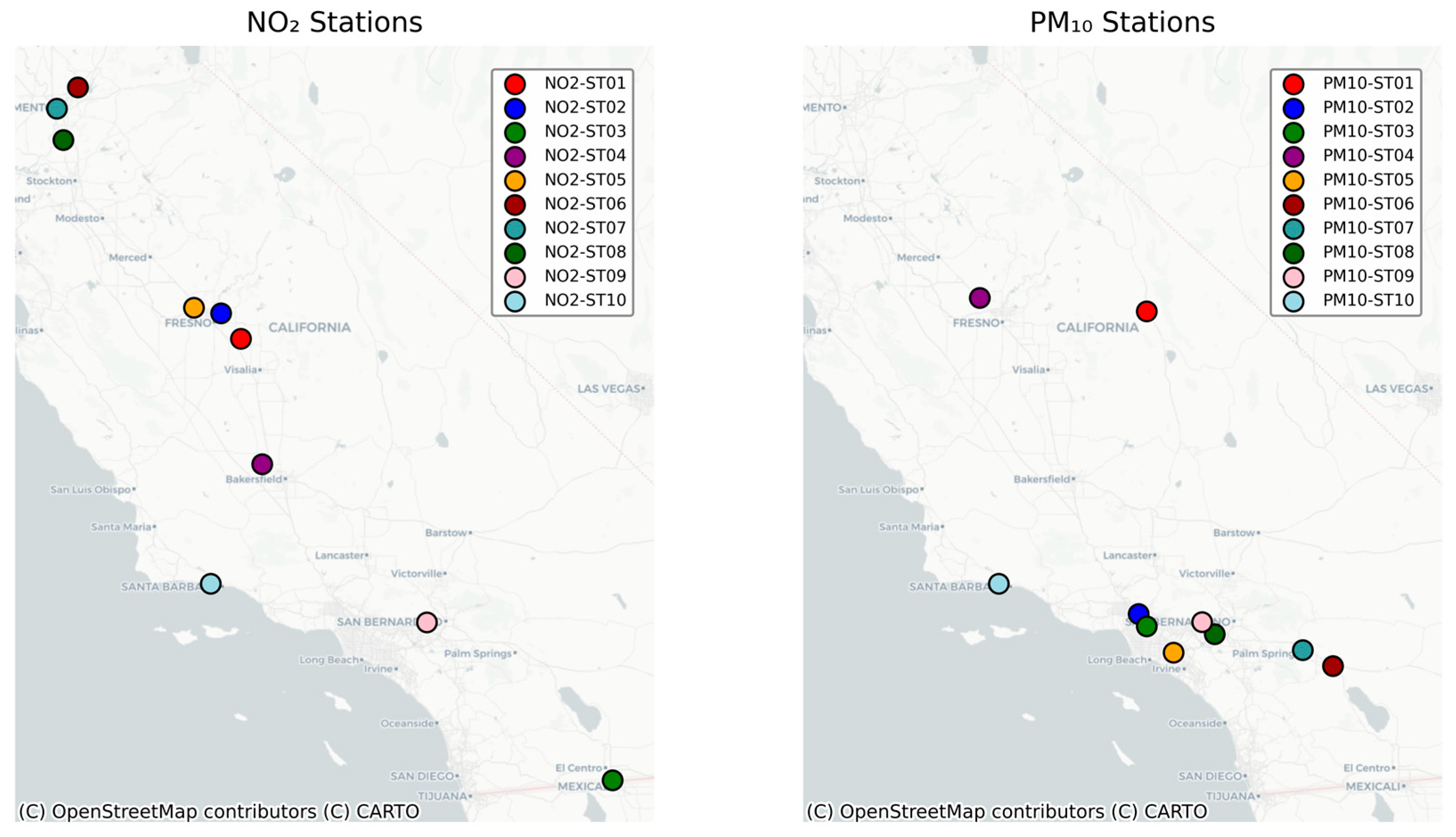Related modeled outputs from the WRF and CMAQ [16,36] models within the EQUATES dataset [37] were also gathered. WRF and CMAQ outputs served as input features for the c (DNN) model to predict meteorological conditions and air quality the following day. This integrated framework, leveraging WRF and CMAQ, enabled a comprehensive approach to air quality forecasting. The stations’ spatial distribution is shown in Figure 1.

Tables S2 and S3 in the Supplementary Material summarize the main characteristics of the hourly NO₂ and PM₁₀ concentration measurements dataset for all stations used, including key statistical properties of pollutants’ concentrations, temperature, and wind speed. All selected monitoring PM₁₀ and NO₂ stations maintained excellent data completeness, by keeping the ones with the highest number of available observations, with each station having more than 60% and 75% of valid measurements throughout the study period for the two compounds, respectively. To achieve that, the data preprocessing firstly determined which stations had concurrent data availability across all required meteorological variables and pollutant parameters. Subsequently, from this subset of common stations, those exhibiting the highest percentage of data completeness were prioritized. Due to a lack of data across the network, the final selection criteria were adjusted to accept the best possible choices.

Based on the station information retrieved from the EPA (Site and Monitor Descriptions, https://aqs.epa.gov/aqsweb/ (accessed on 17 June 2025), the meteorological and pollutant monitoring stations were classified by their geographic coordinates (latitude and longitude). A unique station code was assigned to each site to ensure clear differentiation. This step was necessary because the original EPA AQS metadata did not provide a single, consistent station identifier applicable across all datasets.

The spatial distribution of the 20 selected stations (10 per pollutant; Figure 1) captures key pollution regimes across California: coastal-urban sites (Los Angeles Basin), inland valleys (San Joaquin, Sacramento), and coastal–inland gradients. While this network does not provide uniform spatial coverage, it represents the locations where regulatory monitoring is most dense and where model skill is operationally most important. Spatial representativeness limitations are acknowledged: high-elevation and remote areas remain undersampled, and the network may not fully resolve local-scale gradients in complex terrain. The 5-year period (2010–2014) was selected to balance temporal coverage for deep learning training with meteorological representativeness. This duration captures interannual variability in large-scale patterns and provides an adequate sample size for rare extreme events. While longer periods could improve generalization, the 2010–2014 window avoids confounding from major wildfire seasons post-2015 and represents stable emission-inventory conditions following the 2008 recession.

Data Quality Checks and Treatment of Qualified Values

All hourly pollutant and meteorological records were taken from the EPA’s original AQS site files (site metadata, sample measurement qualifiers, and uncertainty/precision fields). Records with explicit “invalid” qualifiers (for example, flags indicating instrument malfunction or collocated-test failures) were removed. For observations with non-missing measurement values but with either (a) a missing uncertainty field, (b) a qualifier indicating smoke/fire influence, ‘suspect’ or other non-fatal flags, or (c) a missing qualifier, we retained the measured concentration in the analysis. These records were included in model training and evaluation, as due to no EPA warnings, they were considered as real atmospheric conditions (e.g., wildfire-driven peaks) that the bias-correction model must handle operationally.

2.2. Data Preprocessing—Feature Engineering

Comprehensive feature engineering was implemented to enhance predictive capabilities, including Fourier transformations to capture periodic fluctuations at multiple temporal scales (daily, weekly, seasonal), trigonometric time encoding to preserve temporal cyclicity, and statistical aggregates (24-h rolling mean, max, min, standard deviation) of meteorological and air quality variables. Additionally, local statistics and gradients were calculated for 4-h moving windows to detect rapid changes and evolving trends. All features were normalized to [0, 1] range using MinMaxScaler v1.2.2. This prevents numerical instability and preserves relative distributions. The 5-year dataset allowed a 60–20–20 temporal split with 60% of the dataset used for training (2010–2012), 20% for validation (2013), and 20% for testing (2014). This way, we ensured that our validation and training periods encompassed peak pollution seasons.

The feature engineering framework was in direct alignment with the design idea implemented in our bias-correction pipeline. Both current observations and next-day WRF forecasts were included, allowing the model to distinguish between present-state conditions (“now”) and projected meteorological evolution (“tomorrow”). This design enhances lead-time predictive skill. Rolling statistical aggregates (8-h and 24-h windows) capture short-term pollutant persistence and diurnal variability. Fourier features explicitly encode periodicity across daily, weekly, monthly, and annual cycles, a critical factor for resolving the California air quality characteristic variability.

The 60–20–20 temporal split ensures chronological separation of model evaluation and prevents information leakage between time segments. This approach is an extended temporal framework of our previous ozone bias-correction work in Texas [35]. Also, the chosen period (2010–2014) signifies stable emission trends and meteorological conditions that precede the intense wildfires after 2015 [7], providing a representative baseline for bias correction under typical pollution dynamics. The choice of temporal splitting over station-based (spatial) cross-validation was aimed at maintaining realistic operational forecast conditions, where the model must predict future time periods at monitored locations. Station-based splitting would test spatial generalization but is less relevant for bias-correction applications where CMAQ outputs are available at all grid cells. Temporal splitting also preserves station-specific error patterns in training, allowing the model to learn location-dependent biases that arise from local emission characteristics and topographic effects. The trade-off is limited assessment of spatial transferability; future work could evaluate performance at withheld stations to quantify spatial generalization.

During model training, the loss function was computed in the scaled space. The characteristic Huber threshold (δ) and under-prediction penalty parameters were initially derived from physical-unit uncertainties (e.g., ppb, µg m⁻³) and then linearly mapped into the normalized target domain. This way, we maintained the physical interpretability of the loss formulation. In each model train, δ was station-specific (as detailed in Section 2.3.3).

2.3. DNN Model Overview

This section introduces the deep neural network architecture developed for pollutant-specific bias correction. It describes the base CNN–Attention–LSTM architecture that forms the foundation of both models, then details the distinct loss function formulations designed for NO₂ and PM₁₀, the hyperparameter selection methodology and a sensitivity analysis conducted for the tail-gating parameters.

2.3.1. Base CNN–Attention–LSTM Architecture

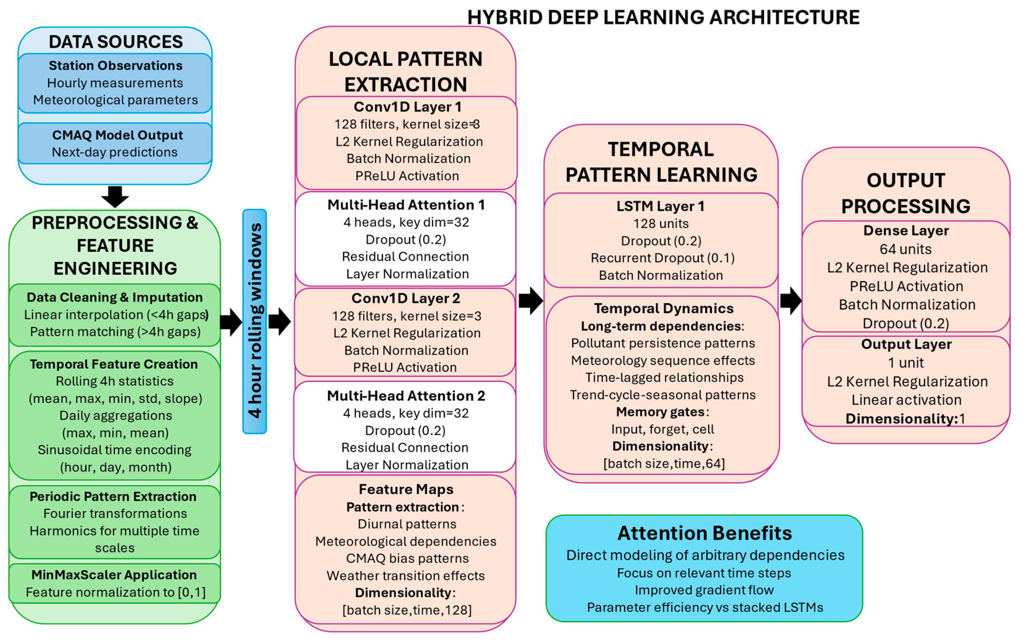
Our forecasting model employs a hybrid deep neural network integrating Convolutional Neural Networks (CNNs), multi-head attention mechanisms, and Long Short-Term Memory (LSTM) layers. This enables capturing both spatial and temporal dependencies within multivariate air quality time series, addressing the natural complexity of meteorological and pollutant dynamics.

The model architecture comprises the following key components: (1) Two 1D Convolutional (Conv1D) layers, each with 128 filters and kernel sizes of 5 and 3, respectively, that can extract localized temporal–spatial features from the multivariate input series. After each convolutional layer, we apply batch normalization to stabilize training, followed by a PReLU activation, whose learnable parameters help the network capture both positive and negative responses. (2) Two multi-head self-attention blocks (4 heads with key dimension 32) enable the model to dynamically focus on relevant time steps when generating predictions. These attention mechanisms are integrated with residual connections and layer normalization (ε = 1 × 10⁻⁶) to facilitate gradient flow and training stability. (3) A single LSTM layer with 128 units models long-range temporal dependencies, configured without sequence return to produce a fixed-size representation. (4) One dense layer (64 units) with PReLU activation and batch normalization integrates high-level representations before the final scalar output. The model is presented in Figure 2.

2.3.2. Loss Function Formulations

Model performance is directly affected by loss function choice, especially for extreme-event detection; we therefore employed distinct loss functions optimized for each pollutant.

For NO₂, we use the standard Huber loss with a data-driven $\delta$ which was estimated for each station from the 2010–2012 training residual $e=y-\widehat{y}$. We computed ${\delta }_{raw}=1.345·s$ with $s=1.4826·MAD\left(y-\widehat{y}\right)$, then converted to the MinMax-scaled target space ${\delta }_{scaled}={\delta }_{raw}/\left(y_{max}-y_{min}\right)$. This ties the quadratic-to-linear transition to the observed error scale while preserving robustness to outliers [38,39]. $y$ represents the observed concentration, $\widehat{y}$ is the model prediction and MAD is the Median Absolute Deviation:

$$L_{Huber}\left(y,\widehat{y}\right)=\left\{\begin{array}{c}{\displaystyle \frac{1}{2}}{\left(y-\widehat{y}\right)}^2,if\vee y-\widehat{y}\vee \le \delta \\ \delta \left(\left|y-\widehat{y}\right|-{\displaystyle \frac{1}{2}}\delta \right),otherwise\end{array}\right.$$

The Huber loss combines the benefits of mean squared error (MSE) for small errors with mean absolute error (MAE) for large errors, providing robustness against outliers while maintaining differentiability. For NO₂, this balanced approach effectively handles both typical conditions and moderate excursions since its concentrations follow relatively predictable diurnal patterns with occasional spikes.

For PM₁₀, we introduce a tailored weighted Huber loss with tail-weighting (gated) mechanism specifically designed to address episodic high-pollution events. The loss function incorporates three key innovations:

The base weighted Huber loss is formulated as:

$$L_{weighted}\left(y,\widehat{y}\right)=L_{Huber}\left(y,\widehat{y}\right)\times w_{tail}\times w_{under}+{\lambda }_{bias}\times \overline{e_{batch}}$$

This formulation adapts robust M-estimator principles [38] by introducing concentration-dependent weighting—a modification motivated by PM₁₀’s episodic nature and public-health significance. While the base Huber loss and percentile-based weighting are established techniques, their combination with asymmetric underprediction penalties and batch-level bias constraints represents a pollutant-specific adaptation not previously documented for air-quality bias correction. The batch bias penalty ${\lambda }_{bias}$= 0.02 constrains systematic drift through the term ${\lambda }_{bias}$ × $\overline{e_{batch}}$. This regularization term prevents the model from shifting predictions upward to minimize asymmetric penalties, maintaining long-term calibration. Where $e=\widehat{y}-y$ is the prediction error, $\overline{e_{batch}}$ is the mean error across the batch and the tail weight $w_{tail}$ smoothly transitions based on observed concentrations:

$$w_{tail}=1+a{\left({\displaystyle \frac{max\left(0,y-q_{90}\right)}{q_{99}-q_{90}}}\right)}^{\gamma }$$

Here, $q_{90}$ and $q_{99}$ represent the 90th and 99th percentiles of training data, $a$ controls maximum weight amplification, and $\gamma$ determines transition sharpness. With this formulation, prediction errors during extreme events ($y$ > $q_{90}$) receive progressively higher weight, reaching maximum amplification (1 + $a$) at the 99th percentile. The underprediction penalty $w_{under}$ specifically targets false negatives during high-pollution episodes:

$$w_{under}=\left\{\begin{array}{c}1+\left(underpen-1\right),ife<0\wedge y>q_{90}\\ 1,otherwise\end{array}\right.$$

where underpen provides an additional penalty for underprediction during tail events. This asymmetric treatment reflects the greater public health consequences of missing pollution episodes versus false alarms. Finally, the batch bias penalty ${\lambda }_{bias}\left|\overline{e_{batch}}\right|$ constrains the model to remain calibrated across concentration ranges by preventing upward changes in mean predictions.

This multi-component loss function addresses several challenges in PM₁₀ forecasting: (1) Extreme Event Focus: The tail-gating mechanism ensures the model offers sufficient capacity to learn patterns that precede high-pollution events. (2) Balanced Performance: The base Huber component maintains accuracy for typical conditions, while the weighting scheme prevents the overlooking of rare but critical episodes. (3) Reduced False Negatives: The asymmetric underprediction penalty directly attends to the cost imbalance in forecast errors, improving sensitivity to pollution episodes. (4) Training Stability: The batch bias regularization prevents systemic solutions where the model simply predicts high values to minimize weighted losses, ensuring meaningful predictions across all concentration ranges.

2.3.3. Hyperparameter Selection and Justification

For the NO₂ model, we employ station-specific Huber thresholds δ calibrated to local measurement characteristics. Thresholds are estimated from robust residual scales (δ ≈ 1.345·σ, with σ from MAD and applied in the scaled target space used for training; in original units, the median δ corresponds to roughly ~1 ppb NO₂, consistent with regulatory QA objectives [40,41]. This identifies that uncertainty varies across sites due to differences in local pollution regimes, maintenance, and environmental conditions that affect monitor performance.

For the PM₁₀ model, δ values are likewise station-specific and optimized from robust residual scales. In original units, they typically fall near ~1–3 μg m⁻³ (≈5–10% of local mean concentrations), aligning with Federal Equivalent Method (FEM) monitor specifications and EPA data-quality goals [41]. This station-specific parameterization follows promising practice in deep learning bias correction for air-quality models, where location-aware hyperparameter tuning improves predictive skill—particularly for sudden extremes—in comparison to single-global settings [23,34].

The tail-gating parameters were determined through a sensitivity analysis:

α = 2.0 (weight amplification factor) was chosen from the range [2, 16] to provide sufficient weight on extreme events without overwhelming the gradient signal from normal conditions. This value ensures that errors at the 99th percentile receive 3× the weight of errors below the 90th percentile. This is based on analysis showing that PM₁₀ extreme events occur approximately 10% of the time, but contribute disproportionately to health impacts [13]. With α = 2.0, tail weight caps at (1 + α) = 3.0 at P99 (base = 1.0 below P90).

$\gamma$ = 2.5 (transition sharpness) was selected from [0.5, 3.0] to create a smooth but decisive transition between normal and extreme regimes. Linear transition ($\gamma$ = 1.0) proved too gradual and $\gamma$ > 2.0 created training instabilities due to sharp gradient changes. The value 2.5 follows similar choices in robust statistics for M-estimators with smooth influence functions [42].

underpen = 1.1 (10% underprediction penalty) reflects epidemiological evidence that health impacts from PM₁₀ exposure follow a supralinear dose–response relationship [14], making underprediction during high-pollution events particularly costly. Values from 1.1 to 1.5 were tested, with 1.1 providing the best F1 score for episode detection without sacrificing overall RMSE.

${\lambda }_{bias}$ = 0.02 was selected through validation-set grid search over [0.001, 0.005, 0.01, 0.02, 0.05]. This value balances two competing objectives: (1) preventing systematic positive bias inflation (which would occur with ${\lambda }_{bias}$ → 0), and (2) minimizing interference with the primary loss signal (requiring ${\lambda }_{bias}$ << 1). The chosen value ensures the bias penalty contributes < 2% to total loss magnitude under typical conditions, following standard regularization practice where auxiliary terms should be 1–2 orders of magnitude smaller than the main objective [43]. Theoretical justification follows from Lagrangian optimization: the penalty acts as a soft constraint enforcing E[y − ŷ] ≈ 0 across mini-batches, preventing the asymmetric loss from creating upward drift.

2.3.4. Sensitivity Analysis of Tail-Gating Hyperparameters

Hyperparameter optimization was conducted on the 2013 validation set using automated grid search. For each configuration, models were trained on 2010–2012 data and evaluated across all PM₁₀ stations. The sensitivity analysis tested α ∈ {2, 4, 8, 12, 16}, γ ∈ {1.0, 1.5, 2.0, 2.5, 3.0}, and underpen ∈ {1.1, 1.2, 1.3, 1.4, 1.5} on the 2013 validation set at all PM₁₀ stations, yielding 125 total configurations per station and optimizing a multi-metric objective (mean rank over RMSE, RMSEs, RMSEu, R², IoA, DTW, and F1). Across stations, higher α increased F1 but degraded calibration and DTW. $\gamma$ = 3.0 occasionally produced training oscillations while values in [2.0, 2.5] concentrated learning near P90–P99 without instability. Across stations, underpen = 1.1 yielded the highest mean F1 at similar recall but lower positive bias than ≥1.3, matching the intended cost asymmetry. The triplet (α, $\gamma$, underpen) = (2.0, 2.5, 1.1) achieved the best aggregate rank, delivering the strongest systematic error reduction with improved F1 and DTW relative to α ≥ 4 or underpen ≥ 1.3. Cross-station generalizability analysis (Table S4) reveals that the optimal configuration (α = 2.0, $\gamma$ = 2.5, underpen = 1.1) appears in the top-10 performing configurations at 90% of stations, despite independent optimization at each location. This generalizability, combined with 83% of all top-3 configurations showing universal applicability (appearing in ≥70% of stations), validates that the selected parameters represent a fundamental optimal region rather than station-specific tuning. Full grids and station-wise ranks are reported in Table S4 and Figures S1 and S2 in the Supplementary Material. All performance results reported in Section 3 are evaluated on the independent 2014 test set, which was not used during hyperparameter tuning.

2.4. Performance Metrics

To assess the proposed deep neural network model, we implemented statistical evaluation metrics that provide insights into predictive capabilities, bias correction efficiency, and ability to capture complex pollutant temporal patterns.

The primary evaluation metric employed was Root Mean Square Error (RMSE), which quantifies the overall magnitude of prediction errors while giving greater weight to larger deviations. To gain a deeper understanding of the model performance characteristics, RMSE was decomposed to systematic RMSE (RMSEs) and unsystematic RMSE (RMSEu). This enables differentiation between consistent prediction biases (RMSEs) and random variability (RMSEu) that cannot be explained by the model. High systematic errors typically indicate calibration issues or structural model deficiencies. High unsystematic errors suggest limitations in capturing data variability due to noise or insufficient model complexity. The Coefficient of Determination (R²) assessed the model’s capacity to explain variance in observed concentrations, with values approaching unity indicating superior predictive capability. Model agreement was evaluated using the Index of Agreement (IoA), which measures the degree to which predicted values correspond with observed measurements.

To evaluate peak-event detection, we used the F₁ score based on a coherent, percentile-based event definition. For each pollutant and station, the 90th percentile (T90) of the training-set observations was used as the episode threshold. Hours with concentrations y ≥ T90 were labeled as “events.” This station-specific threshold normalizes for regional differences in baseline levels while ensuring that the tail coverage matches the weighting used in the loss function. Class imbalance (≈1:9 event-to-non-event ratio) was addressed through a 2× sample weight for tail values and the asymmetric under-prediction penalty term in the Tail-Weighted Huber loss (Section 2.3.2), which jointly prioritize accurate reproduction of high-concentration episodes. Validation F₁, precision, and recall were then computed from these binary event labels to quantify the model’s ability to detect extreme pollution episodes.

To assess the temporal pattern alignment, we used the Dynamic Time Warping (DTW) [44,45] distance. It measures the optimal alignment between predicted and observed time series while accommodating non-linear temporal shifts. An essential metric for evaluating how well the model captures the timing and sequencing of pollution episodes.

This evaluation framework spans simple error measures to advanced temporal pattern analyses, providing comprehensive validation of the bias correction method. Mathematical definitions of all metrics are given in Table S1 of the Supplementary Material.

3. Results and Discussion

Performance improvements differ between pollutants due to their distinct atmospheric behavior and CMAQ error characteristics. PM₁₀’s superior correction reflects the effectiveness of the weighted Huber loss in capturing episodic events poorly represented in CMAQ (e.g., dust storms, stagnation periods), whereas NO₂’s more moderate gains suggest that remaining errors stem from sub-grid emission variability and rapid photochemical transformations that exceed the model’s temporal resolution. These results align with recent DL bias-correction studies [29,32,35] but extend them through pollutant-specific loss functions tailored to event characteristics rather than uniform architectures applied across species.

3.1. Performance Metric Evaluation

The developed hybrid deep neural network significantly improved performance across all evaluated performance metrics compared to the CMAQ calculations for both NO₂ and PM₁₀ concentrations. Our evaluation included twenty monitoring stations: ten for NO₂ (NO2-ST01 through NO2-ST10) and ten for PM₁₀ (PM10-ST01 through PM10-ST10), with consistent improvements observed across diverse atmospheric and pollution conditions. Detailed results from the chunk-based analysis illustrating the temporal evolution of bias correction performance at each monitoring station are presented in the supplementary material as figures (Figures S3–S12 for NO₂ and Figures S13–S22 for PM₁₀).

3.2. RMSE Analysis and Error Decomposition

RMSE decomposition into systematic (RMSEs) and unsystematic (RMSEu) components quantifies the model’s ability to correct persistent biases versus random variability. Systematic error reflects long-term mean biases (e.g., consistent underestimation due to missing emission sources or inadequate boundary-layer mixing), while unsystematic error captures event-to-event variability.

Table 1. Summary of RMSE improvements across NO₂ and PM₁₀ monitoring networks.

Metric	NO2 (Mean ± Std)	PM10 (Mean ± Std)
RMSE reduction (%)	50.99 ± 11.69	48.57 ± 18.57
RMSEs reduction (%)	79.88 ± 26.49	94.32 ± 4.54
RMSEu reduction (%)	42.42 ± 6.95	32.81 ± 19.56

summarizes mean improvements across stations.

3.2.1. NO₂ Model Performance

The model significantly outperformed the CMAQ baseline across all NO₂ monitoring stations, achieving RMSE reductions ranging from 33.02% to 71.03%. The most substantial improvement was observed at station NO2-ST01, where RMSE decreased from 9.44 to 2.73, yielding a 71.03% improvement. Station NO2-ST07 showed the most modest but still significant improvement, with RMSE reducing from 6.14 to 4.12, a 33.02% improvement. These results demonstrate the model’s robust ability to reduce overall prediction errors across diverse spatial conditions and varying baseline NO₂ concentration levels.

Spatial analysis reveals that coastal-urban stations (NO₂-ST01, ST04) achieved greater RMSE reductions (>60%) than inland valley sites (NO₂-ST06, ST08: 33–45%), likely reflecting stronger diurnal forcing and more predictable boundary-layer dynamics in coastal regimes. The substantial systematic error correction (80–99%) indicates the model successfully learned to compensate for CMAQ’s persistent underestimation during morning rush-hour peaks and stable nocturnal conditions—biases that arise from coarse temporal resolution of emission inventories and inadequate representation of shallow nighttime mixing.

The decomposition of RMSE into systematic (RMSEs) and unsystematic (RMSEu) components revealed exceptionally strong bias correction capabilities, as presented in Figure 3. Systematic error reduction was outstanding across all stations. Improvements ranged from 16.96% to 99.28%. Station NO2-ST03 exhibited the highest systematic bias correction, with RMSEs decreasing from 6.51 to 0.047, representing a 99.28% improvement. Even station NO2-ST05, which showed the lowest systematic improvement, achieved a 16.96% reduction in RMSEs. Regarding unsystematic error correction, the model achieved RMSEu improvements ranging from 30.66% to 51.96%, with station NO2-ST09 demonstrating the highest random error reduction at 51.96%.

3.2.2. PM₁₀ Model Performance

The PM₁₀ bias correction model achieved RMSE reductions ranging from 17.70% to 80.21%. The most substantial improvement was observed at station PM10-ST03, where RMSE decreased from 22.01 to 4.94, a 80.21% improvement. Station PM10-ST06 showed the most modest improvement with a 17.70% RMSE reduction. The systematic error correction for PM₁₀ was exceptional, with improvements ranging from 83.94% to 98.65%. Station PM10-ST09 achieved the highest systematic bias correction at 98.65%, while station PM10-ST07 showed the lowest but still substantial improvement at 83.94%. For unsystematic errors, PM₁₀ model improvements ranged from 4.64% to 78.73%, with station PM10-ST03 demonstrating the highest random error reduction. Figure 4 presents the RMSE improvements for each station.

The near-complete systematic bias reduction (94.32% average) demonstrates that the weighted Huber loss effectively corrected CMAQ’s tendency to underpredict high-concentration episodes. Stations at higher elevations (PM₁₀-ST09: 480 m) showed slightly lower improvements (36%) compared to valley sites (PM₁₀-ST03, ST05: 70–80%), suggesting that complex terrain amplifies local emission and transport processes not fully captured by CMAQ’s 12-km resolution. The lower unsystematic error reduction (33% vs. 42% for NO₂) reflects PM₁₀’s inherently more stochastic behavior driven by episodic sources (dust, wildfires, long-range transport) that challenge even advanced DL architectures.

3.3. Model Explanatory Power and Agreement Metrics

R² and Index of Agreement (IoA) quantify the model’s ability to reproduce observed variability and temporal patterns. R² measures the proportion of variance explained. IoA assesses magnitude and phase agreement without penalizing systematic bias as heavily as R². These metrics complement RMSE decomposition by revealing whether bias correction improves the model’s representation of diurnal cycles, synoptic variability, and episodic events.

3.3.1. Coefficient of Determination (R²) Performance

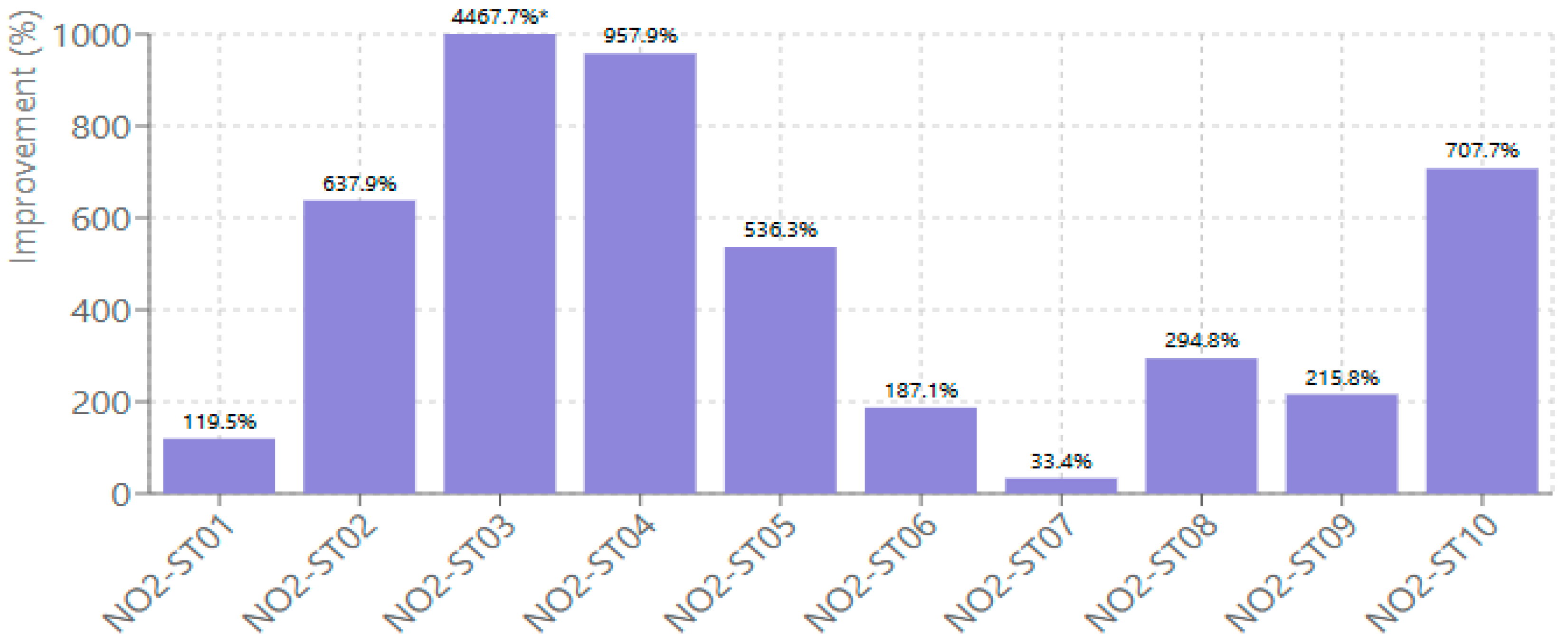
The R² improvements demonstrated the models’ enhanced explanatory power across both pollutants (Figure 5). For NO₂ predictions, R² enhancements ranged from 33.40% to 4467.71%. Station NO2-ST03 achieved the most substantial improvement, increasing from −0.016 to 0.70, which represents a 4467.71% enhancement that transformed a baseline model with negative explanatory power into one with strong predictive capability. The large percentage improvements (hundreds to thousands of percent) reflect the mathematical property that R² gains are amplified when baseline values are near zero or negative. For instance, improving from R² = −0.016 to 0.70 represents a 4468% increase but, more meaningfully, indicates transformation from no predictive skill (worse than climatology) to strong explanatory power (70% of variance explained). Negative baseline R² values indicate CMAQ predictions are less skillful than simply using the mean concentration, highlighting the critical need for bias correction. Station NO2-ST07 showed the most modest but still meaningful improvement of R² at 33.40%.

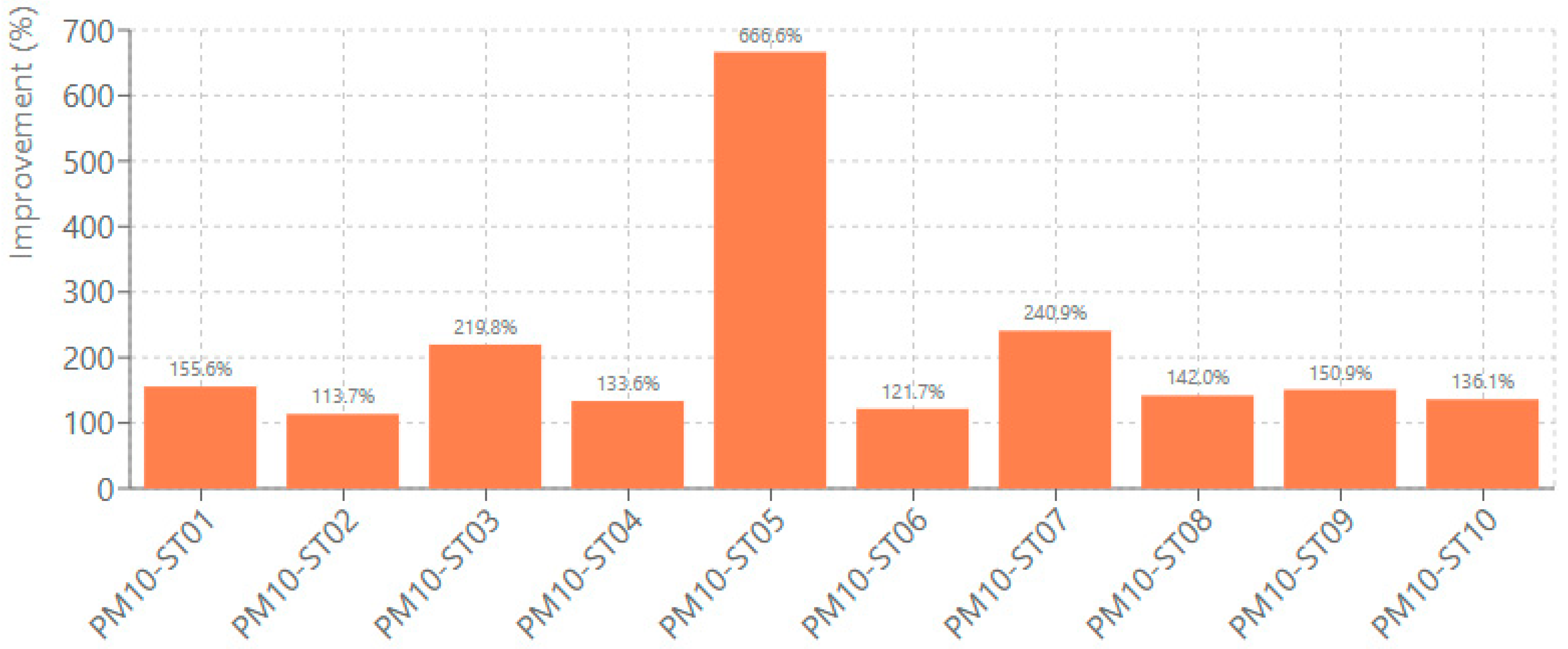
PM₁₀ predictions showed R² improvements ranging from 113.70% to 666.59% (Figure 6). Station PM10-ST05 achieved the best improvement, increasing from −0.090 to 0.501, a 666.59% correction. Station PM10-ST02 demonstrated the most conservative but still substantial R² improvement at 113.70%. These significant improvements across both pollutants indicate that the bias correction approach fundamentally enhances the models’ capacity to capture underlying patterns in atmospheric concentration data. While PM₁₀ improvements are smaller in percentage terms compared to NO₂, the absolute gains in R² are comparable. The difference reflects higher baseline R² values for PM₁₀ (mostly positive), suggesting CMAQ captures PM₁₀ temporal variability better than NO₂, likely because PM₁₀ exhibits slower atmospheric evolution and stronger persistence that coarse-resolution CTMs can represent.

3.3.2. Index of Agreement (IoA) Enhancements

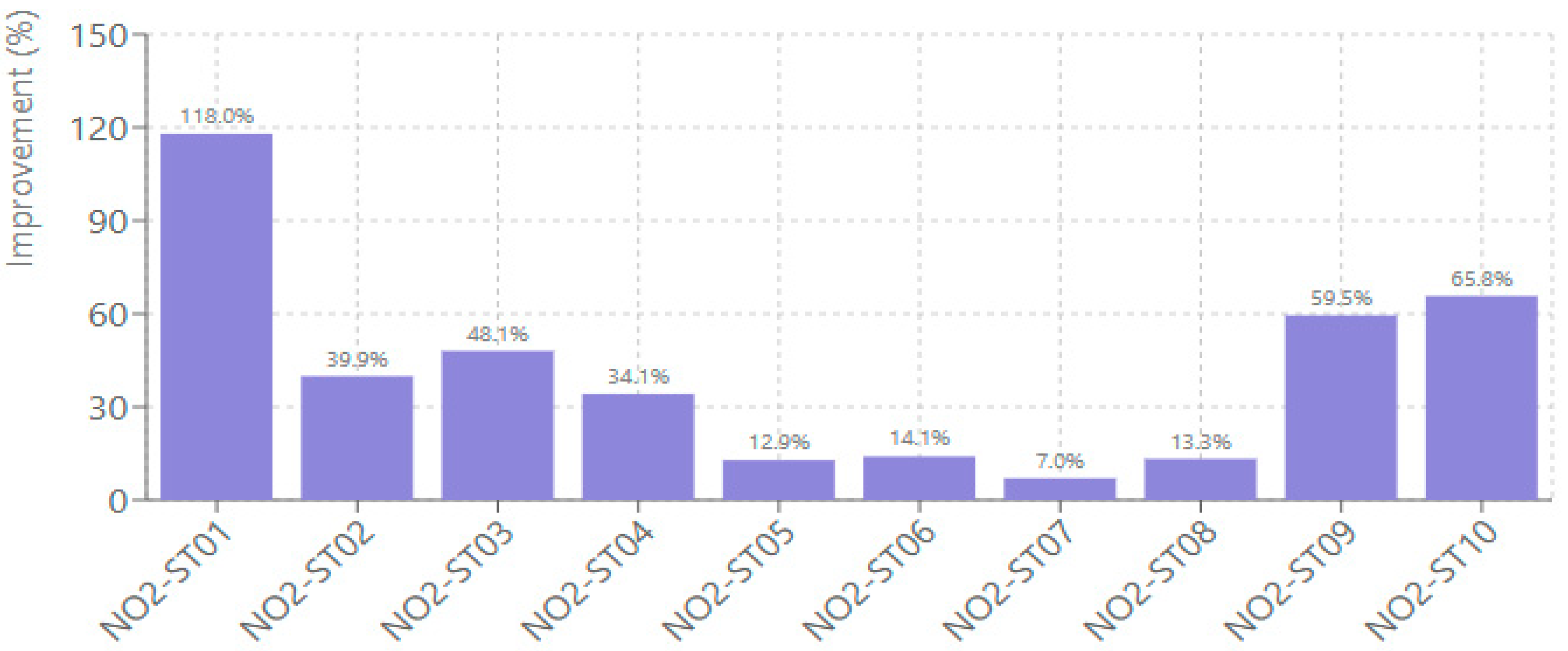
Index of Agreement improvements varied between the two pollutants, reflecting their different atmospheric behavior patterns. NO₂ predictions showed IoA improvements ranging from 7.02% to 118.02% (Figure 7), with station NO2-ST01 achieving the highest enhancement from 0.41 to 0.89. Station NO2-ST07 showed the most modest improvement at 7.02%. The IoA improvements indicate enhanced reproduction of temporal patterns, including diurnal cycles (morning rush-hour peaks, afternoon photochemical maxima) and day-to-day variability driven by synoptic meteorology. IoA gains are smaller than R² gains because IoA already penalizes phase errors and magnitude mismatches, making it a more conservative metric where CMAQ had moderate baseline skill (NO₂: 0.41–0.89; PM₁₀: 0.28–0.56).

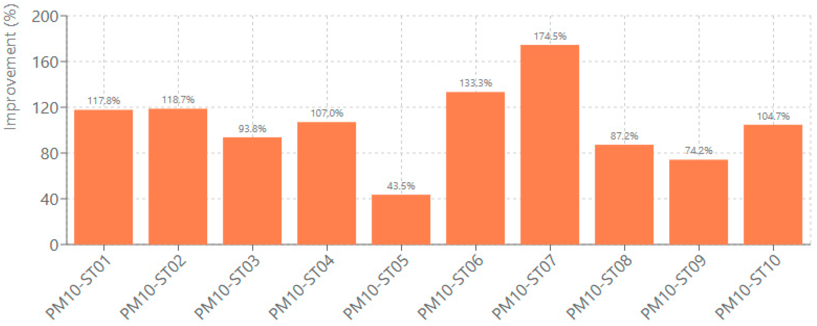
PM₁₀ predictions showed IoA improvements ranging from 43.54% to 174.51%, with station PM10-ST07 achieving the highest enhancement, from 0.28 to 0.73 (Figure 8). The consistently higher IoA improvements for PM₁₀ compared to NO₂ suggest that the bias correction approach is particularly effective for addressing systematic discrepancies in particulate matter predictions. PM₁₀’s substantially larger IoA improvements (+105% vs. +41% for NO₂) directly relate to the weighted Huber loss function. By emphasizing extreme events (P₉₀–P₉₉), the loss forces the model to correctly time episodic peaks—the most challenging feature for pattern-matching metrics. This pollutant-specific optimization demonstrates that tailoring loss functions to atmospheric behavior (episodic vs. continuous) yields metric-specific gains: PM₁₀ excels in temporal agreement (IoA, DTW), while NO₂ shows broader gains across all metrics due to its more predictable diurnal structure.

3.4. Temporal Alignment and Event Detection Performance

3.4.1. Dynamic Time Warping (DTW) Analysis

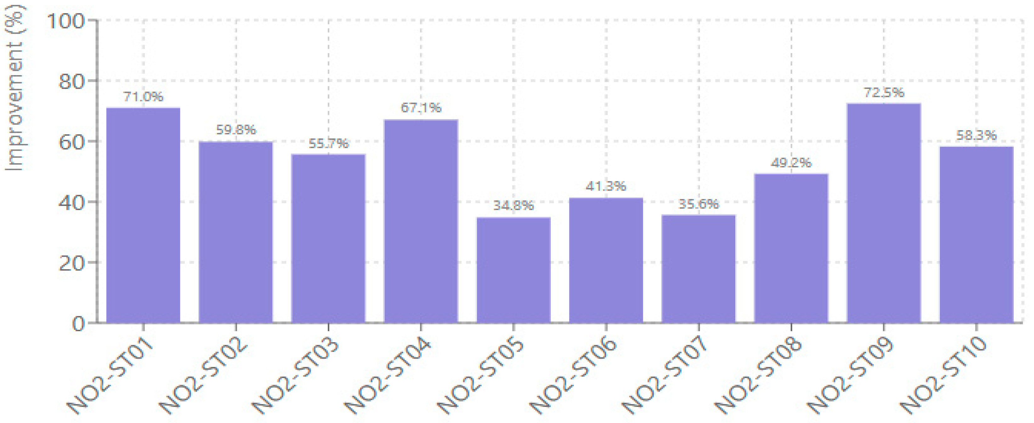
DTW distance improvements, shown in Figure 9, indicate enhanced temporal alignment between predicted and observed concentrations. NO₂ predictions achieved DTW improvements ranging from 34.80% to 72.47%, with station NO2-ST09 demonstrating the highest. Station NO2-ST05 showed the smallest but still meaningful DTW enhancement of 34.80%. DTW distance is measured in concentration units (ppb for NO₂, μg/m³ for PM₁₀) and quantifies the cumulative alignment cost when optimal time-shifts are allowed. For NO₂, DTW distance decreased from an average of 4.52 ppb (CMAQ) to 2.21 ppb (DNN), representing 56% improvement in temporal alignment. This indicates the model reduced phase errors (timing mismatches of pollution peaks) by approximately 1–2 h in diurnal cycles, better capturing morning rush-hour onset and afternoon photochemical maxima timing.

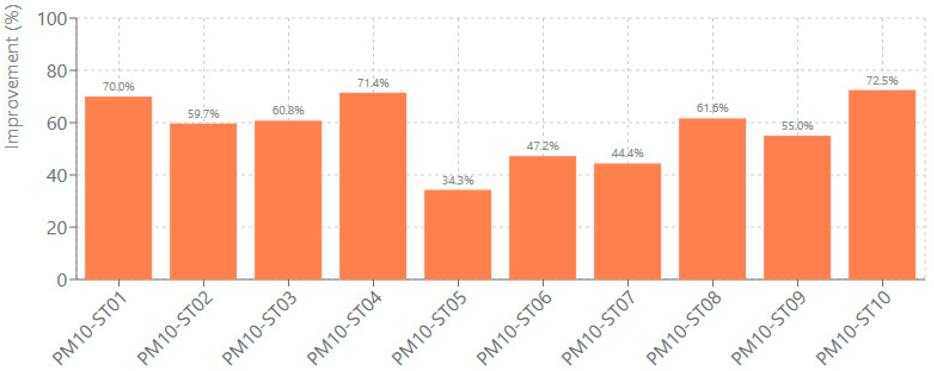
PM10 predictions showed DTW improvements ranging from 34.28% to 72.47%, with station PM10-ST10 achieving the highest temporal alignment improvement (Figure 10). For PM₁₀, DTW distance decreased from an average of 9.07 μg/m³ (CMAQ baseline) to 4.31 μg/m³ (DNN), quantifying the improved temporal alignment in concentration units. These substantial DTW reductions across both pollutants indicate significantly enhanced temporal alignment between predicted and observed concentrations, a vital result for operational forecasting applications. The comparable DTW improvements for both pollutants (55–58% average) demonstrate that the hybrid architecture successfully learned temporal phasing regardless of pollutant chemistry, suggesting that meteorological drivers (boundary-layer height evolution, wind patterns) dominate timing errors in CMAQ rather than chemical mechanisms.

3.4.2. F1 Score Performance for Peak Detection

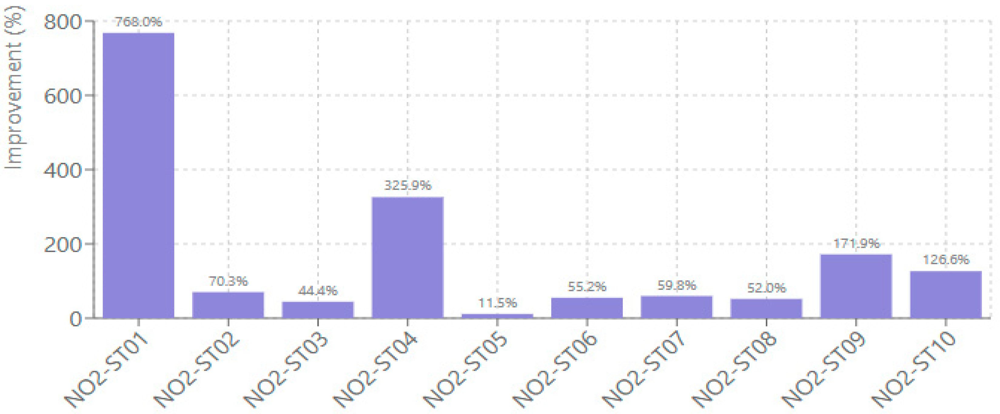
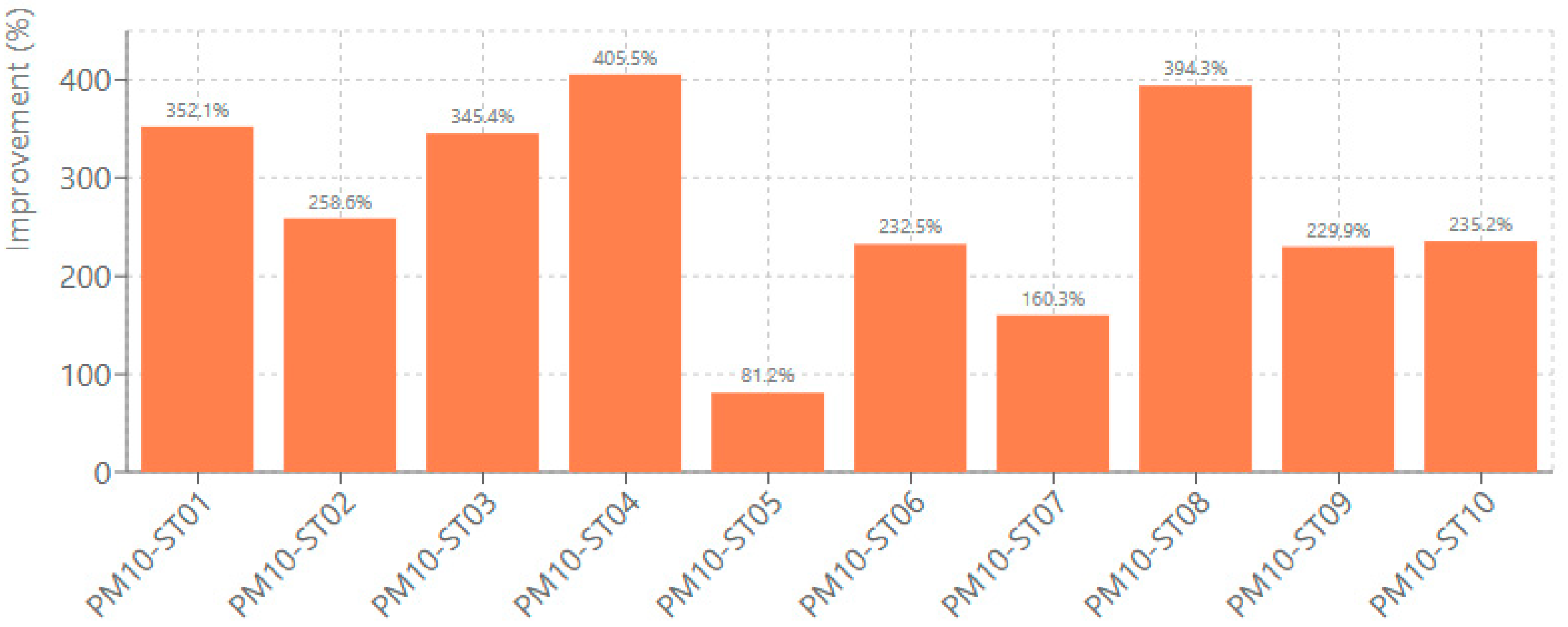
F1 score improvements, which are essential for assessing peak pollution event detection capabilities, varied considerably across stations and pollutants, as presented in Figure 11. NO₂ predictions showed F1 score improvements ranging from 11.51% to 768.02%. Station NO2-ST01 exhibited the largest enhancement from 0.031 to 0.272, representing a 768.02% improvement in peak detection accuracy. Station NO2-ST05 showed the smallest F1 score improvement at 11.51%.

Despite large percentage gains, absolute F1 scores remain moderate (typically 0.25–0.45), indicating that extreme NO₂ event detection remains challenging. The model succeeds during synoptic stagnation events with regional-scale accumulation. It struggles, though, with isolated urban hotspots driven by sub-grid emission variability and rapid, localized processes that CMAQ’s 12-km resolution cannot fully resolve.

PM₁₀ predictions demonstrated F1 score improvements ranging from 81.19% to 405.49% (Figure 12). Station PM10-ST04 achieved the highest F1 score enhancement from 0.065 to 0.327, representing a 405.49% improvement. Station PM10-ST05 showed the most conservative but still substantial improvement at 81.19%. These semantic improvements in event detection across both pollutants are particularly valuable for air quality warning systems and public health applications.

PM₁₀’s higher absolute F1 scores reflect the weighted loss function’s explicit optimization for tail events. The remaining moderate absolute values (0.24–0.47 range) suggest that extreme PM₁₀ prediction remains challenging, likely due to the episodic nature of sources and limitations in CMAQ’s spatial resolution for capturing localized emission variability.

3.5. Comparative Performance Analysis

This section synthesizes the bias correction performance across both pollutants, firstly examining systematic error reduction and then presenting the overall performance assessment across all metrics.

3.5.1. Systematic Bias Correction Effectiveness

Averaged across all stations, the systematic bias correction (RMSEs) showed significant performance for both pollutants. NO₂ predictions achieved an average systematic error reduction of 79.88%, ranging from 16.96% to 99.28% across stations. PM₁₀ predictions demonstrated an even higher systematic bias correction, averaging 94.32% improvement, with a range from 83.94% to 98.65%. The strong systematic bias correction for PM₁₀ reflects the model’s effectiveness in addressing the complex emission uncertainties and atmospheric chemistry processes that particularly affect PM₁₀ predictions.

3.5.2. Overall Performance Assessment

The complete evaluation across twenty monitoring stations confirms the effectiveness of our hybrid CNN-LSTM architecture for both NO₂ and PM₁₀ bias correction. NO₂ predictions achieved average improvements of 50.99% in RMSE, 815.80% in R², 41.27% in IoA, 54.53% in DTW distance, and 168.56% in F1 score. PM₁₀ predictions demonstrated average improvements of 48.57% in RMSE, 208.08% in R², 105.48% in IoA, 57.67% in DTW distance, and 269.50% in F1 score.

The random error correction (RMSEu) averaged 42.42% for NO₂ and 32.80% for PM₁₀, indicating enhanced capability to capture unpredictable atmospheric variability for both pollutants. These consistent improvements across all evaluated metrics and monitoring stations demonstrate that deep learning approaches can significantly enhance the reliability and accuracy of chemical transport model outputs for multiple pollutant types.

The reported performance is based on temporal validation (2014 test set) at stations used during training. While the model demonstrates consistent skill across diverse California sites with varying pollution regimes and topography, true spatial generalizability would require evaluation at completely withheld monitoring locations not seen during training. The lack of independent spatial validation means we cannot definitively claim transferability to unmonitored regions or other geographic domains.

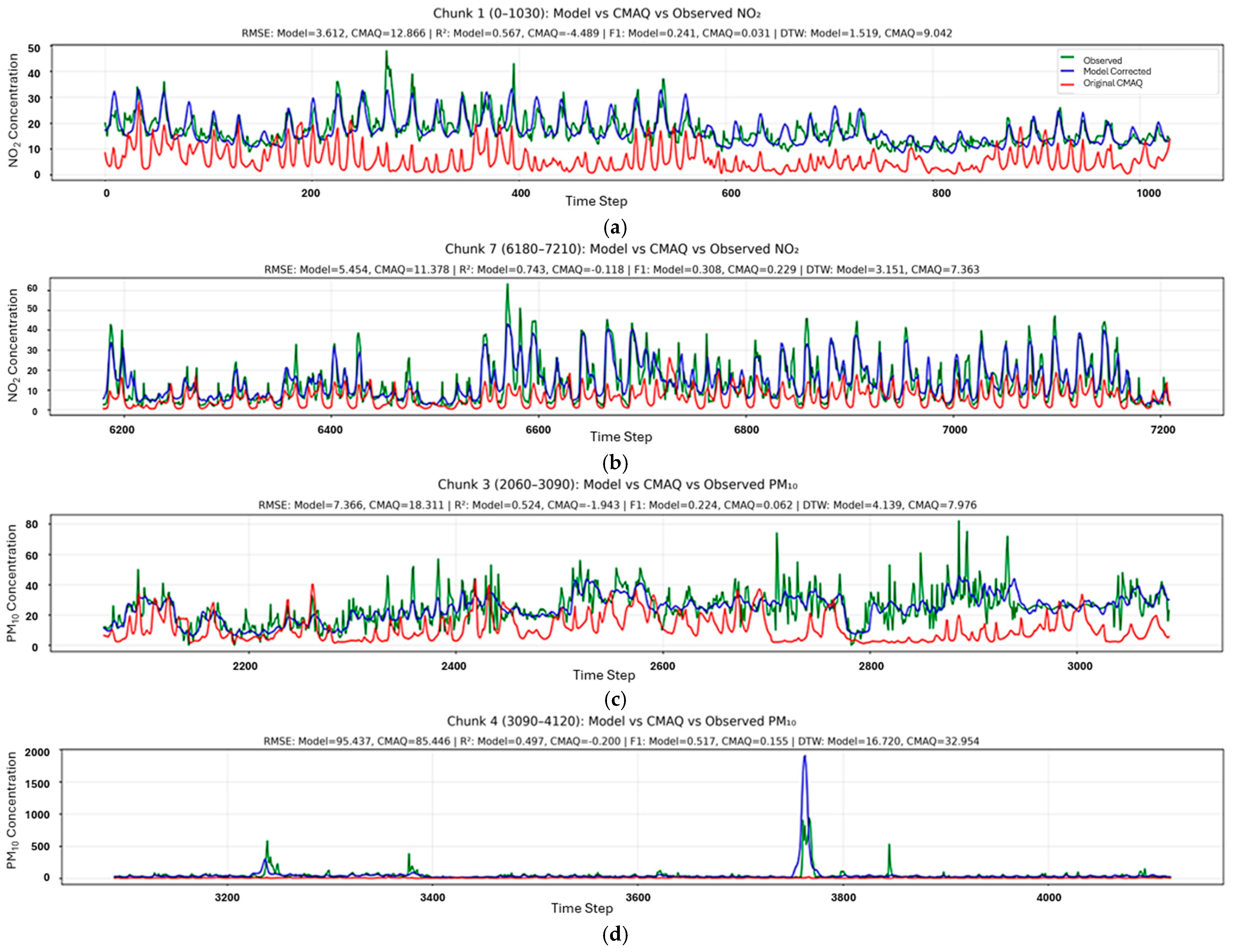
To provide intuitive insight into model behavior across diverse conditions, Figure 13 presents representative hourly time series segments for four stations spanning California’s distinct spatial regimes. For NO₂, station NO2-ST01 (Figure 13a), located in the coastal-urban environment of the San Francisco Bay Area, exemplifies the correction of systematic CMAQ overprediction: the original CTM consistently overestimates concentrations by 5–15 ppb throughout the diurnal cycle—likely due to the model’s underestimation of sea breeze dispersion effects—while the bias-corrected predictions closely track observed values, reducing RMSE from 12.87 to 3.61 ppb. Station NO2-ST03 (Figure 13b), situated in California’s Central Valley where topographic barriers trap pollutants and promote accumulation, demonstrates the model’s ability to capture high-concentration episodes characteristic of this region, with multiple peaks reaching 50–60 ppb accurately reproduced (R² = 0.74) despite CMAQ’s substantial underestimation of these events.

For PM₁₀, the contrast between typical valley conditions and extreme fire-influenced episodes is particularly instructive. Station PM10-ST02 (Figure 13c), a suburban-agricultural site in the northern Central Valley, shows a sustained period of elevated concentrations (~40–60 μg/m³) where CMAQ systematically underestimates observed values; the bias-corrected model successfully captures both the magnitude and temporal evolution of this episode typical of valley pollution accumulation. Station PM10-ST06 (Figure 13d), located in fire-prone inland Southern California, presents an extreme case: a pollution event reaching approximately 2000 μg/m³—consistent with wildfire smoke transport common in this region—where both CMAQ and the corrected model struggle with absolute accuracy due to the exceptional magnitude. Nevertheless, the bias-corrected model substantially improves event detection (F1 score: 0.52 vs. 0.16 for CMAQ), demonstrating that the tail-weighted loss function enhances the model’s ability to identify extreme episodes even when precise concentration prediction remains challenging. This station corresponds to PM10-ST06, which exhibited the highest SHAP amplification factors during extreme events (Section 3.7.2), confirming the mechanistic link between feature attribution patterns and operational performance under challenging environmental conditions.

3.6. Spatial Heterogeneity and Model Robustness

Station-specific analysis revealed distinct performance patterns across the monitoring networks. For NO₂ predictions, stations NO2-ST01 and NO2-ST09 consistently demonstrated the greatest improvements across multiple metrics, while stations NO2-ST05 and NO2-ST07 showed more conservative but still meaningful enhancements. For PM₁₀ predictions, station PM10-ST03 achieved notable performance across error reduction metrics, while station PM10-ST07 excelled in agreement metrics.

Spatial analysis reveals that coastal-urban stations (within 30 km of the Pacific coast) achieved 10–15% higher average RMSE reductions compared to inland valley sites, likely reflecting more predictable diurnal forcing from sea-breeze circulations and better-constrained boundary-layer dynamics in CMAQ’s meteorological inputs. Urban core stations (Los Angeles, Sacramento metro areas) showed superior systematic bias correction (>85%) compared to suburban/rural sites (65–75%), suggesting that emission inventory quality—which receives greater refinement in densely monitored urban areas—directly impacts the learnable bias structure.

The spatial divergence in performance improvements emphasizes the importance of location-specific factors in air quality modeling. Factors like local emission patterns, topographical influences, and meteorological complexities. However, the consistent improvements across all twenty stations and all seven metrics confirm the robust applicability of the deep learning approach across diverse environmental conditions for both NO₂ and PM₁₀ predictions.

These results establish that the hybrid CNN-LSTM bias correction methodology provides a reliable and general approach for enhancing chemical transport model outputs across different pollutant types. They offer significant improvements in forecast accuracy, temporal alignment, and peak event detection, capabilities that are essential for operational air quality management systems.

Although elevation was not included explicitly as a model feature, its indirect influence was evident across station-specific performance patterns. For the PM₁₀ network, the highest-elevation site PM₁₀_ST01 (Independence, Inyo County, 1201 m) exhibited smaller absolute RMSE values but moderate skill (R² ≈ 0.62, IoA ≈ 0.73). This reflects the low concentration variability, which is typical of desert–mountain environments. In contrast, low-elevation urban and suburban sites such as PM₁₀_ST02 (Burbank), PM₁₀_ST03 (Los Angeles), and PM₁₀_ST04 (Madera) achieved higher explained variance (R² = 0.70–0.78) and RMSE reductions exceeding 50%.

For the NO₂ network, elevated or topographically complex stations such as NO2_ST09 (Fontana, 381 m) showed slightly reduced normalized skill compared with valley and urban stations, including NO2_ST01 (Parlier), NO2_ST02 (Clovis), and NO2_ST06 (Roseville). These trends suggest that elevation affects model performance mainly through its relationship with local meteorology and how well emissions are represented, rather than acting as a strong predictor on its own. This is consistent with the uneven pattern of improvements observed across California.

3.7. Feature Attribution Analysis

To complement the quantitative performance assessment and provide mechanistic insight into model behavior, we conducted feature attribution analysis using SHapley Additive exPlanations (SHAP) [46,47]. The GradientExplainer algorithm [48] was applied across all 20 stations (10 NO₂, 10 PM₁₀), with 1000 background samples establishing baseline expectations and 800 test samples explained per station. Beyond overall feature importance, we separately analyzed attribution patterns under normal conditions versus extreme events (>90th percentile concentrations) to investigate whether the models adaptively adjust their feature weighting during high-concentration episodes. This distinction is particularly relevant for evaluating the tail-weighted loss function’s impact on PM₁₀ predictions, as effective bias correction during pollution episodes is critical for public health applications.

3.7.1. Overall Feature Importance

Table 2. Mean SHAP feature importance (%) across all stations for NO₂ and PM₁₀.

Rank	NO2 Feature	NO2 (%)	PM10 Feature	PM10 (%)
1	Obs. Daily Mean	31.0 ± 4.1	Obs. Daily Mean	30.0 ± 8.9
2	Wind	7.6 ± 3.4	Fourier Sin 24 h	7.2 ± 2.4
3	Fourier Sin 24 h	6.8 ± 1.6	Hour Sin	6.0 ± 2.4
4	CMAQ Conc	5.1 ± 3.0	Fourier Cos 24 h	5.7 ± 3.2
5	Hour Sin	4.8 ± 1.2	Hour Cos	5.1 ± 1.8
6	CMAQ Daily Mean	4.3 ± 1.4	Temp 8 h Mean	4.4 ± 2.8
7	Hour Cos	4.1 ± 1.5	CMAQ Bias 8 h Mean	4.3 ± 2.0
8	Rh Dp	3.4 ± 0.8	CMAQ Conc	3.8 ± 1.7
9	CMAQ Bias 8 h Mean	3.0 ± 0.8	Rh Dp	3.5 ± 1.4
10	Fourier Cos 24 h	3.3 ± 0.9	WRF Temp Next 24 h	3.2 ± 1.1

presents the mean SHAP-derived feature importance across all stations for both pollutants, expressed as percentage contributions to the total attribution. For NO₂, observed daily mean concentration emerged as the dominant predictor (31.0% ± 4.1%), appearing in the top five features at all 10 stations. This strong persistence signal reflects the regular diurnal patterns of traffic-related NO₂ emissions and the autocorrelated nature of urban air quality. Wind speed ranked second (7.6% ± 3.4%), consistent with the critical role of atmospheric dispersion in modulating ground-level NO₂ concentrations from local vehicular sources. The diurnal Fourier component (Fourier Sin 24 h) contributed 6.8%, capturing the characteristic morning and evening concentration peaks associated with rush-hour traffic.

For PM₁₀, persistence similarly dominated (30.0% ± 8.9%), though with notably higher station-to-station variability (coefficient of variation: 30% versus 13% for NO₂). This heterogeneity reflects the diverse source profile of particulate matter across California, encompassing urban emissions, agricultural dust, wildfire smoke, and regional transport. In contrast to NO₂, wind speed contributed only 1.6% to PM₁₀ predictions—a five-fold reduction that underscores the fundamental difference in source characteristics. While NO₂ originates predominantly from local traffic and is therefore sensitive to local dispersion conditions, PM₁₀ concentrations are influenced by multiple sources operating across different spatial scales, reducing the predictive value of local wind measurements.

Temporal and seasonal features exhibited greater importance for PM₁₀ than NO₂. The combined contribution of Fourier components reached 19.2% for PM₁₀ compared to 12.1% for NO₂, reflecting the stronger diurnal amplitude associated with boundary layer dynamics and the pronounced seasonal patterns driven by wildfire activity and winter inversion climatology. Similarly, WRF meteorological forecasts contributed 6.8% for PM₁₀ versus 4.0% for NO₂, indicating that future meteorological conditions—particularly temperature and humidity—provide greater predictive value for particulate matter, likely through their influence on secondary aerosol formation and atmospheric stability.

Despite these differences, CMAQ-derived features contributed similarly for both pollutants (12.4% for NO₂, 12.7% for PM₁₀), demonstrating that the bias correction architecture effectively leverages CTM outputs regardless of pollutant species. The CMAQ Bias 8 h Mean feature, which encodes recent systematic model errors, ranked within the top 10 for both pollutants, confirming that the network learns to identify and correct persistent CTM biases. The results for the feature category contributions are summarized in

Table 3. Feature category contributions (%) for NO₂ and PM₁₀.

Category	NO2 (%)	PM10 (%)	Difference
Historical/Persistence	33.2	37.0	+3.8
Current Meteorology	25.9	20.8	−5.1
Temporal Encoding	17.1	23.2	+6.1
Fourier (Seasonality)	12.1	19.2	+7.1
CMAQ Predictions	12.4	12.7	+0.3
WRF Forecasts	4.0	6.8	+2.8

.

3.7.2. Feature Importance During Extreme Events

To investigate whether the models adapt their prediction strategy during high-concentration episodes, we compared SHAP attributions between normal conditions and extreme events, defined as observed concentrations exceeding the 90th percentile.

Table 4. Feature importance amplification during extreme events (>90th percentile).

Feature	NO2 Ratio	PM10 Ratio	Interpretation
CMAQ Bias 8 h Mean	2.59	2.61	CTM underestimation amplifies
Obs. Daily Mean	2.02	2.16	Persistence strengthens
Month Cos	2.59	1.68	Seasonal clustering (NO2 > PM10)
Day Cos	2.30	1.66	Weekly patterns (NO2 > PM10)
Hour Cos	1.75	1.73	Diurnal timing
Rh Dp	1.89	1.61	Humidity effects
Wind	1.65	1.09	Dispersion (NO2 only)
Fourier Sin 24 h	1.40	1.25	Diurnal cycle stable

presents the ratio of mean absolute SHAP values during extreme versus normal conditions for key features. Ratios exceeding 1.0 indicate features that gain importance during pollution episodes, while ratios below 1.0 indicate diminished relevance.

The most striking finding was the consistent amplification of CMAQ Bias 8 h Mean importance during extreme events for both pollutants: 2.59× for NO₂ and 2.61× for PM₁₀. This near-identical amplification across fundamentally different pollutant species provides direct evidence that CMAQ systematically underestimates high concentrations, and that the bias correction network learns to compensate more strongly during these episodes. The physical interpretation is clear: when observed concentrations are elevated, the discrepancy between CMAQ predictions and reality is larger, and the model correctly identifies historical bias patterns as the most informative feature for correction.

Persistence (Obs. Daily Mean) also amplified during extremes, with ratios of 2.02× for NO₂ and 2.16× for PM₁₀. This reflects the autocorrelated nature of pollution episodes, which typically persist over multiple hours or days due to stagnant meteorological conditions. The slightly higher amplification for PM₁₀ is consistent with the multi-day character of wildfire smoke events and regional particulate pollution episodes.

Notable differences emerged between pollutants in the amplification patterns of other features. For NO₂, temporal features showed substantial amplification: Month Cos (2.59×) and Day Cos (2.30×), indicating that extreme NO₂ events cluster preferentially in certain seasons (winter) and days (weekdays). Wind importance also increased during NO₂ extremes (1.65×), as calm conditions are a necessary precursor to concentration buildup from traffic sources. In contrast, PM₁₀ showed more modest amplification of these features (Month Cos: 1.68×, Wind: 1.09×), suggesting that extreme PM₁₀ events are driven by a more diverse set of meteorological and source conditions.

One station, PM10-ST06, exhibited exceptional amplification factors that merit discussion. At this site, Obs. Daily Mean importance increased 5.18× during extremes—the highest value across all 20 stations—while CMAQ Bias 8 h Mean showed 6.79× amplification. Additionally, the 720-h (monthly) Fourier components, which capture seasonal patterns, amplified by 5.02× and 3.77× for cosine and sine components, respectively. This combination suggests that PM10-ST06 experiences severe, persistent pollution episodes with pronounced seasonal clustering, likely associated with wildfire impacts or terrain-enhanced inversions. The extreme CMAQ bias amplification indicates that the CTM particularly underperforms at this location during high-concentration events, and the model has learned correspondingly strong bias corrections. This station exemplifies the conditions under which the tail-weighted loss function provides maximum benefit: where CTM errors are largest precisely when accurate predictions matter most for public health protection. Station’s PM10-ST06 amplification factors are presented in

Table 5. Extreme amplification factors at PM10-ST06.

Feature	Normal	Extreme	Ratio
CMAQ Bias 8 h Mean	0.00025	0.00170	6.79
Obs. Daily Mean	0.00415	0.02152	5.18
Fourier Cos 720 h	0.00031	0.00158	5.02
Fourier Sin 720 h	0.00037	0.00138	3.77
Hour Cos	0.00134	0.00433	3.24
Month Sin	0.00068	0.00180	2.63

.

The observed amplification patterns provide mechanistic validation for the pollutant-specific loss function design. The 2.6× increase in bias correction importance during extremes demonstrates that the model requires stronger gradient signals for high-concentration samples to learn appropriate corrections. The tail-weighted Huber loss function, which applies asymmetric penalties emphasizing underprediction of elevated concentrations, directly addresses this requirement by ensuring that extreme events contribute proportionally more to the training objective. The SHAP results thus connect the architectural design choices to observable model behavior, confirming that the bias correction mechanism operates as intended.

4. Conclusions

This study demonstrates that pollutant-specific deep learning architectures can substantially improve chemical transport model predictions when they are tailored to the atmospheric behavior of individual species. By developing distinct CNN–Attention–LSTM models with optimized loss functions for NO₂ and PM₁₀, we achieved consistent bias corrections across 20 California monitoring stations, with systematic error reductions of roughly 80% for NO₂ and over 90% for PM₁₀. The key advance lies not in architectural complexity, but in pollutant-specific design: standard Huber loss for the smoother, more predictable temporal patterns of NO₂, and a weighted, tail-gated Huber loss for the episodic, heavy-tailed behavior of PM₁₀. This differentiation outperformed uniform deep learning frameworks applied identically across species.

PM₁₀ exhibited greater systematic bias reduction and stronger agreement with observations (IoA improvement > 100%), driven by the enhanced weighting of extreme events. In contrast, NO₂ achieved larger improvements in random-error reduction and explanatory power, reflecting its smoother diurnal cycle and more predictable photochemical evolution. These results suggest that multi-species bias correction benefits more from pollutant-specific optimization architecture.

The model improvements translate directly to more reliable air quality forecasts. Systematic bias reductions provide more accurate baselines for regulatory assessments, while substantial gains in peak-event detection (F₁ score increases of approximately 170% for NO₂ and 270% for PM₁₀) enhance early-warning capabilities during high-exposure episodes. Improvements in temporal alignment (DTW reductions around 50–60%) reduce diurnal phase errors that can otherwise undermine operational forecasting during rush-hour NO₂ peaks or afternoon PM₁₀ maxima. Together, these advances strengthen the utility of CMAQ outputs.

Limitations remain. First, validation used a temporal holdout at stations included during training; full spatial generalizability requires evaluation at monitoring sites withheld entirely from training. Second, constraints inherent to the 12-km CMAQ grid—such as coarse emission inventories and unresolved sub-grid processes—cannot be overcome solely by statistical post-processing. Third, despite the interpretive value of attention mechanisms, the models remain largely black-box, limiting mechanistic insight into emissions, meteorology, or chemistry errors within the underlying CTM.

Our future work could follow several directions. First, we could extend the pollutant-specific methodology to PM_2.5. As a pollutant, it has similar characteristics to PM₁₀ but also presents distinct health impacts. Second, it is important to test how well the trained models can be transferred in time. In other words, we should examine whether they keep their accuracy when applied to periods that differ strongly from the training years, especially under changing emissions and climate conditions. In this context, incorporating large-scale climate anomaly indicators, such as El Niño–Southern Oscillation (ENSO) indices, represents a promising extension, as these variables influence drought persistence, wildfire activity, and interannual variability in particulate matter concentrations, particularly in California. Third, exploring ensemble approaches that combine predictions from multiple bias-corrected models could further enhance forecast accuracy and quantify prediction uncertainty for decision support.

A particularly promising direction could be the development of spatial deep learning architectures that extend CMAQ bias correction across diverse geographic regions, including areas that lack monitoring stations. Such an approach could leverage Graph Neural Networks (GNNs) to capture spatial dependencies between monitoring locations by incorporating topographical features, land use patterns, and meteorological conditions. Using transfer learning techniques, models trained on data-rich regions could be adjusted to areas with limited monitoring infrastructure. This could significantly expand the impact of bias correction methodologies for large-scale air quality assessment.

Integrating additional data sources represents another important possibility for advancement. Incorporating satellite observations (e.g., TROPOMI for NO₂, MODIS for aerosol optical depth) could provide spatial constraints and validation data between monitoring stations. Also, high-resolution emission inventories, mainly for mobile sources and industrial facilities, could improve local-scale predictions. Other meteorological products, like radar-derived boundary layer heights and lidar measurements of aerosol vertical profiles, could enhance the model’s ability to capture atmospheric mixing and transport processes that affect both NO₂ and PM₁₀ concentrations.

Despite the substantial improvements demonstrated in this study, deep learning models present challenges that deserve careful consideration. The main limitation is the risk of overfitting. This is especially important when the models are applied to new regions or unusual meteorological conditions. Dropout regularization, batch normalization, and early stopping with episode-level callbacks can help reduce this risk. However, it is of great importance to validate the models on independent datasets. DNN models depend strongly on the training data, they must be tested carefully before being used in new locations or time periods, particularly in regions with different emission profiles, topography, or meteorological patterns.

The black-box nature of deep learning models, despite attention mechanisms that provide some interpretability, limits our ability to identify specific physical processes or error sources in the underlying chemical transport model. The systematic error decomposition helps separate bias from random error, but it does not show whether the errors come from emissions, meteorology, chemistry, or other inputs. This is a limitation that emphasizes the fact that bias correction should be seen as a complement to, not a replacement for, continued improvement of chemical transport models and their input data.

Although this study does not directly quantify health outcomes, the demonstrated improvements in bias reduction, peak detection, and temporal alignment have direct implications for respiratory-health protection and air-quality management. Both NO₂ and PM₁₀ are strongly associated with acute respiratory morbidity, hospital admissions, and premature mortality, particularly during short-term pollution episodes [13,14]. In particular, the substantial gains in peak-event detection and temporal alignment directly address the forecast attributes that are most critical for protecting respiratory health during short-term exposure episodes. The reductions in systematic bias, combined with gains in F1 score and Dynamic Time Warping performance, indicate a markedly improved ability to anticipate not only the magnitude but also the timing of high-exposure events. Accurate timing is critical for operational warning systems, as even 1–2 h phase errors can substantially reduce the effectiveness of public-health advisories and exposure-mitigation measures.

From a policy and decision-making perspective, the enhanced detection of episode days enables earlier and more reliable activation of short-term interventions, such as public health alerts, traffic and industrial emission controls, advisories for sensitive populations (e.g., children, elderly individuals, and individuals with asthma or chronic obstructive pulmonary disease), and hospital preparedness during forecasted pollution episodes. Improved bias-corrected forecasts also strengthen the use of CMAQ-based products in regulatory applications, including exceedance risk assessment relative to air-quality standards and evaluation of episodic control strategies. In this context, the proposed pollutant-specific bias correction framework serves as a practical bridge between advanced numerical modeling and actionable information for respiratory-health protection.

While the present study does not perform exposure–response or health-impact modeling, the demonstrated forecast improvements represent a necessary upstream condition for reliable health-risk communication and policy response. Future work could directly couple these improved forecasts with established exposure–response functions to quantify avoided respiratory morbidity or hospital admissions under operational warning scenarios.

Key scientific contributions of this study include:

• Demonstration of the fact that pollutant-specific loss functions outperform universal architectures for multi-species bias correction;
• A weighted tail-gated Huber loss enabling significant systematic bias reduction (>90%) and large F₁ improvements for episodic PM₁₀ events;
• Temporal validation confirming consistent skill across diverse California sites;
• RMSE decomposition showing that deep learning corrects both systematic biases (80–94%) and random errors (33–42%), indicating learned atmospheric patterns beyond simple mean-shifting;
• Operational relevance through improved diurnal timing, enhancing real-time forecasting and exposure-mitigation decision-support.

In summary, this study proposes a robust framework for pollutant-specific, AI-driven bias correction in multi-species air quality modeling. We applied tailored CNN–Attention–LSTM architectures with optimized loss functions for NO₂ and PM₁₀. These models show that deep learning can substantially improve chemical transport model outputs while accounting for the different atmospheric behavior and forecasting challenges of each pollutant. We evaluated the approach at twenty monitoring stations using seven performance metrics and systematic error decomposition. This confirmed both the effectiveness and the generalizability of the method. The resulting framework provides a solid basis for reliable multi-species air quality forecasts that can support environmental management and public health decisions. The improvements in bias correction, peak detection, and temporal alignment meet key operational forecasting needs and make the method suitable for integration into real-world air quality management and warning systems.