


Abstract
Public-health respiratory-disease surveillance requires distinguishing expected seasonal illness activity from atypical changes that may warrant further investigation. Weekly influenza-like illness (ILI) data support situational monitoring, retrospective anomaly screening, and short-term forecasting, but these tasks are often conducted using separate statistical baselines. We empirically evaluated whether seasonal–trend decomposition using LOESS (STL) could provide a common interpretable baseline using weekly national U.S. ILI data from 1997 to 2025. Expected activity was represented by the estimated trend plus recurring seasonal component, while residuals represented baseline-adjusted deviations. Residual exceedance and persistence summaries were examined retrospectively, and forecast performance was evaluated through rolling-origin comparisons with SARIMA, seasonal naive, and ETS benchmarks at 4-, 8-, and 12-week horizons. The decomposition highlighted major departures from the recurring annual pattern, including the 2009 H1N1 pandemic and COVID-19-era disruptions. At the 4-week horizon, STL had the lowest RMSE (0.925), slightly below SARIMA (0.929), seasonal naive (1.270), and ETS (1.710). At the 8- and 12-week horizons, seasonal naive performed best, with RMSEs of 1.270 and 1.280, compared with 1.280 and 1.450 for STL. The two-week persistence rule produced no pre-peak warnings at any tested threshold, indicating that retrospective residual screening did not by itself provide effective early warning. The empirical study demonstrates that STL provides a transparent common baseline for linking monitoring, retrospective anomaly screening, and short-term forecasting while distinguishing expected seasonal progression from baseline-adjusted deviations.
1. Introduction
Timely respiratory-disease surveillance requires information on changes in community illness activity before complete laboratory-confirmed data are available. Influenza-like illness (ILI) surveillance provides a timely syndromic measure of outpatient respiratory illness and therefore contributes to public-health situational awareness. National ILI indicators also provide information for healthcare capacity planning and for identifying unusual changes in respiratory illness activity [1,2].
Because ILI is a syndromic indicator, an increase in ILI activity cannot by itself be attributed specifically to influenza. It may also reflect other respiratory infections, changes in healthcare-seeking behavior, or changes in surveillance participation and reporting. In addition, ILI activity follows a strong annual cycle, so a high observed value is not necessarily unusual if it occurs during the expected winter increase. Without a clearly defined baseline, routine seasonal progression may be mistaken for atypical activity, while meaningful departures from expected behavior may be difficult to interpret. A statistical baseline is therefore needed to separate longer-term change and recurring seasonal variation from deviations that may warrant further investigation.
A wide range of statistical methods has been developed for infectious-disease surveillance and influenza monitoring. Classical Serfling-type regression models define expected seasonal behavior and quantify excess activity relative to that baseline [3]. Aberration-detection methods, including Farrington-type algorithms and Early Aberration Reporting System procedures, are designed to flag unusual increases using recent or historical reference periods [4,5,6]. Time-series models, including ARIMA-family models and exponential smoothing, are commonly used for short-term forecasting because they can represent temporal dependence and recurring seasonal patterns [7,8]. Although these approaches are useful for their intended purposes, they generally emphasize individual surveillance objectives, such as alerting or forecasting. Consequently, monitoring, anomaly screening, and forecasting may rely on different statistical representations of expected activity.
This motivates the evaluation of seasonal–trend decomposition using LOESS (STL) as a common interpretable baseline for national ILI surveillance. STL separates an observed time series into trend, seasonal, and residual components [9]. In the present application, the trend and seasonal components represent expected ILI activity, while the residual component represents baseline-adjusted deviation. This decomposition allows routine monitoring, retrospective residual screening, persistence summaries, and short-term forecasts to be interpreted through the same statistical structure on the original ILI percentage scale.
The objective of this study was to evaluate empirically whether an STL-based surveillance baseline could provide such a common baseline for weekly national U.S. ILI data. Specifically, we examined whether the trend and seasonal components could represent expected activity, whether the residual component could summarize retrospective departures from that expectation, and whether the same decomposition could generate competitive short-term baseline forecasts. Forecast performance was evaluated using rolling-origin comparisons with SARIMA, seasonal naive, and ETS benchmarks at 4-, 8-, and 12-week horizons. Residual exceedance and persistence analyses were interpreted retrospectively and were not treated as validated prospective alerting procedures.
The contribution of this study is primarily interpretive and organizational rather than methodological. STL itself is an established decomposition method, and the present analysis is not intended to replace calibrated aberration-detection or probabilistic forecasting systems. Instead, we empirically evaluate whether a transparent decomposition-based baseline can connect monitoring, retrospective anomaly screening, persistence summaries, and short-term forecasting within a common national ILI surveillance structure. The remainder of the paper is organized as follows. Section 2 describes the ILI dataset and preprocessing. Section 3 presents the decomposition, residual-screening, persistence, and forecasting methods. Section 4 reports the empirical results. Section 5 and Section 6 provide the discussion and conclusions.
2. Data
Weekly national ILI data were obtained from the U.S. Centers for Disease Control and Prevention (CDC) through the U.S. Outpatient Influenza-like Illness Surveillance Network (ILINet), accessed via FluView Interactive. The series reports the percentage of outpatient visits meeting the ILI case definition among participating healthcare providers nationwide.
The analysis uses weekly observations from February 1997 through March 2025. Because the analysis was conducted using the nationally aggregated ILI percentage series, no subgroup or group-size parameter was specified in the decomposition. The effect of aggregation level, such as regional or state-level grouping, is therefore outside the scope of the present national-level analysis. ILI is defined as the percentage of outpatient visits with fever (temperature ≥ 37.8 °C) accompanied by cough and/or sore throat, without a known non-influenza cause. As a syndromic indicator, ILI reflects overall respiratory illness activity rather than laboratory-confirmed influenza infection.
The dataset is indexed by epidemiological week and year according to the CDC/MMWR convention used by FluView/ILINet. In this system, weeks run from Sunday to Saturday and are numbered 1–52/53. Reporting was not uniformly available across the full calendar year in the early years, and there are some reporting gaps outside the typical influenza season. To preserve the temporal structure, we constructed a complete regular weekly time index spanning the study period and represented unreported weeks as missing observations rather than removing them. Epidemiological weeks were mapped to week-ending calendar dates for consistent alignment.
Across the complete regular weekly index used in the analysis, there were 1466 weekly time points. Of these, 1340 weeks had observed national ILI values and 126 weeks were missing, corresponding to 8.6% of the weekly index. Missing weeks occurred because reporting was not uniformly available across all weeks in the earlier part of the series and because of occasional reporting gaps.
Missing weeks were handled according to the analysis objective. For descriptive summaries, residual interpretation, residual-based screening, and persistence summaries, only weeks with observed ILI values contributed to the reported results. Unreported weeks were retained as missing and were not interpreted as zero. For STL decomposition and forecasting models that required a complete regular time series, missing values were filled using linear interpolation. Interpolated values were used only to support decomposition, model fitting, and forecast generation; they were not treated as observed validation outcomes or counted as observed residual exceedances or persistence signals.
Week 53 time points were retained in the regular weekly time index. Because the STL and SARIMA models used a fixed 52-week seasonal period, week 53 was not modeled as a separate seasonal category; instead, it was included as part of the continuous weekly sequence. This is a minor approximation of the epidemiological calendar and is acknowledged as a limitation.
The observed weekly ILI percentages showed strong seasonal structure, with relatively low values during most non-peak weeks and substantially higher values during winter epidemic periods and atypical high-activity episodes. Because the objective of the analysis was to separate expected seasonal structure from baseline-adjusted deviations, the primary descriptive display of the series is provided through the STL decomposition in Section 4. We therefore focus the main text on decomposition, residual-threshold, autocorrelation, and forecasting results rather than on marginal distributional diagnostics of the raw ILI series.
3. Methods
The analysis was organized around an STL-based baseline for weekly national ILI activity. The observed ILI series was decomposed into trend, seasonal, and residual components. The trend and seasonal components were used to define expected baseline activity, while the residual component was used to summarize baseline-adjusted deviations. Forecasting performance was evaluated formally using a rolling-origin design. Residual exceedance and persistence rules were used only as retrospective surveillance summaries, not as validated prospective outbreak-alert rules.
3.1. STL Decomposition
Seasonal–trend decomposition using LOESS (STL) was applied to the weekly national ILI percentage series [9]. The additive decomposition was written as
where is the observed ILI percentage in week t, is the trend component, is the seasonal component, and is the residual component.
STL was implemented in R using the stl() function. The seasonal period was set to 52 weeks to represent the annual cycle in weekly ILI activity. The seasonal component was estimated using s.window = "periodic", and robust fitting was used by setting robust = TRUE. Under this specification, the recurring within-year seasonal pattern was treated as stable across years, while the trend component captured slower changes in baseline activity. Missing values were handled as described in Section 2: interpolation was used only when a complete regular time series was required for decomposition or model fitting, and observed weeks were used for residual summaries and forecast-error calculations.
3.2. Interpretability of the Decomposition
Interpretability was defined operationally as the ability to connect each model output to a surveillance meaning on the original ILI percentage scale. The trend component represents longer-term baseline change, the seasonal component represents recurring within-year variation, and the residual component represents baseline-adjusted deviation. Positive residual exceedances therefore indicate weeks with higher-than-expected ILI activity after accounting for the estimated trend and seasonal baseline. This interpretation was used consistently for retrospective residual screening, persistence summaries, and STL-based baseline forecasts.
3.3. Residual-Based Screening
Residual-based screening was used to identify weeks with unusually high ILI activity relative to the STL baseline. A week was flagged when
where is the STL residual, is the mean residual, is the residual standard deviation, and k is a threshold parameter. The main analysis used . The rule was applied only to observed ILI weeks. Because the STL decomposition for this analysis was fitted retrospectively to the full study period, these flags were interpreted as retrospective baseline-adjusted exceedances rather than prospective outbreak detections.
3.4. Persistence-Based Warning Summaries
Persistence-based summaries were used to identify sustained residual exceedances. Let
where is an indicator function. The main persistence rule defined a warning signal when residual exceedances occurred in two consecutive weeks:
The main analysis used and two-week persistence. Sensitivity analyses considered alternative threshold values, including , , and .
Persistence summaries were evaluated retrospectively at the influenza-season level. For each season, the seasonal peak was defined as the observed week with the maximum national ILI percentage. We recorded whether any warning occurred during the season, whether the first warning occurred before the seasonal peak, the lead time from the first pre-peak warning to the peak, and the average number of warning signals per season. Because prospectively adjudicated outbreak labels were not available, these quantities were not interpreted as sensitivity, specificity, or false-positive-rate estimates.
Because this analysis was intended as a retrospective description rather than an operational alert calibration, the persistence definition was fixed at two consecutive exceedances, and sensitivity analysis varied only the residual threshold k. Alternative persistence lengths were not evaluated as alert rules because such calibration would require prospectively defined public-health targets and labeled as outbreak outcomes.
3.5. Short-Term Forecasting and Benchmark Models
Short-term forecasting performance was evaluated using a rolling-origin design at 4-, 8-, and 12-week horizons. At each forecast origin, models were fitted using observations available up to that week, and forecasts were generated for the following horizon. Forecast origins were included only when the full horizon was available. Forecast errors were calculated only for future weeks with observed ILI values.
For the STL-based approach, forecasts were generated by extrapolating the estimated trend component and adding the corresponding seasonal component for each future week. The residual component was treated as having mean zero for point forecasting and was not added directly to the predicted value.
A seasonal ARIMA model was used as a conventional statistical benchmark. SARIMA models were fitted with a seasonal period of 52 weeks and selected using the corrected Akaike Information Criterion [8,10]. For the rolling-origin forecast evaluation, the SARIMA order was re-selected at each forecast origin using only the training observations available up to that week; future validation observations were not used for model selection or fitting. The SARIMA benchmark was evaluated using the same rolling-origin design and the same forecast horizons as the STL-based forecasts.
Two additional benchmark forecasts were included. First, a seasonal naive forecast used the observed ILI percentage from the same week in the previous annual cycle,
this benchmark provides a simple reference model based on annual seasonal persistence. Second, an ETS benchmark was included as an exponential-smoothing reference model [8]. Because the weekly ILI series has a 52-week seasonal period, ETS was implemented as a nonseasonal ETS benchmark, while the seasonal naive forecast served as the explicit annual-seasonal benchmark.
All benchmark methods were evaluated using the same rolling-origin design, forecast horizons, and observed validation weeks. Forecast accuracy was summarized using root mean squared error (RMSE), mean absolute error (MAE), and mean absolute percentage error (MAPE). SARIMA residual diagnostics were assessed using residual plots, autocorrelation functions, and Ljung–Box tests [11].
4. Results
4.1. Descriptive Patterns and Decomposition
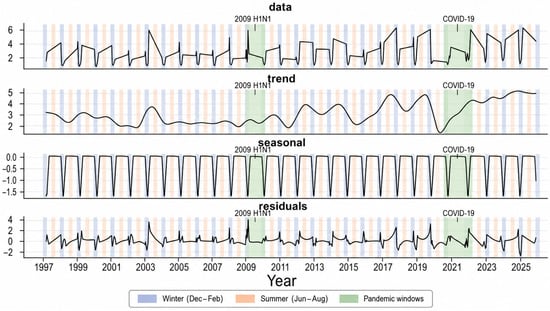
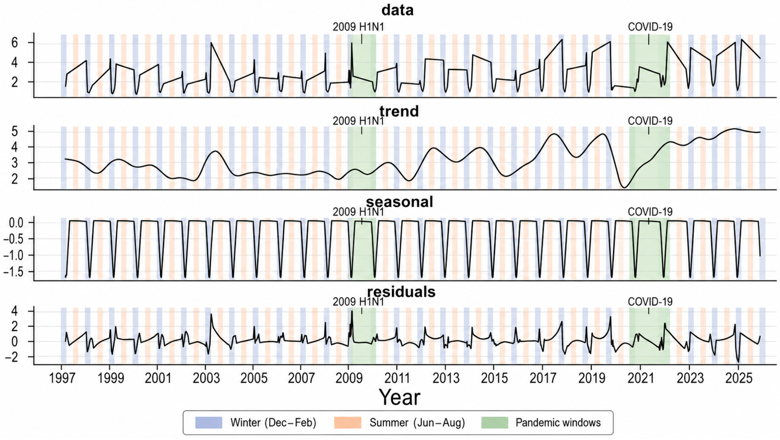
Figure 1 shows the STL decomposition of weekly national ILI into the observed series, trend component, seasonal component, and residual component. The observed series shows a recurring annual pattern, with higher ILI activity generally occurring during winter periods and lower activity during summer periods. The pandemic windows coincide with visible departures from the typical seasonal pattern. The trend component summarizes slower multi-year changes in baseline ILI activity after removing the recurring seasonal pattern. The seasonal component captures the within-year structure of the series, with regular winter increases and summer decreases. The residual component contains the remaining week-to-week variation after subtracting the estimated trend and seasonal components from the observed ILI series.
Figure 1.
STL decomposition of weekly national ILI, with seasonal and pandemic-period shading.
4.2. STL Residual Diagnostics for Retrospective Screening
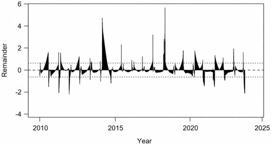
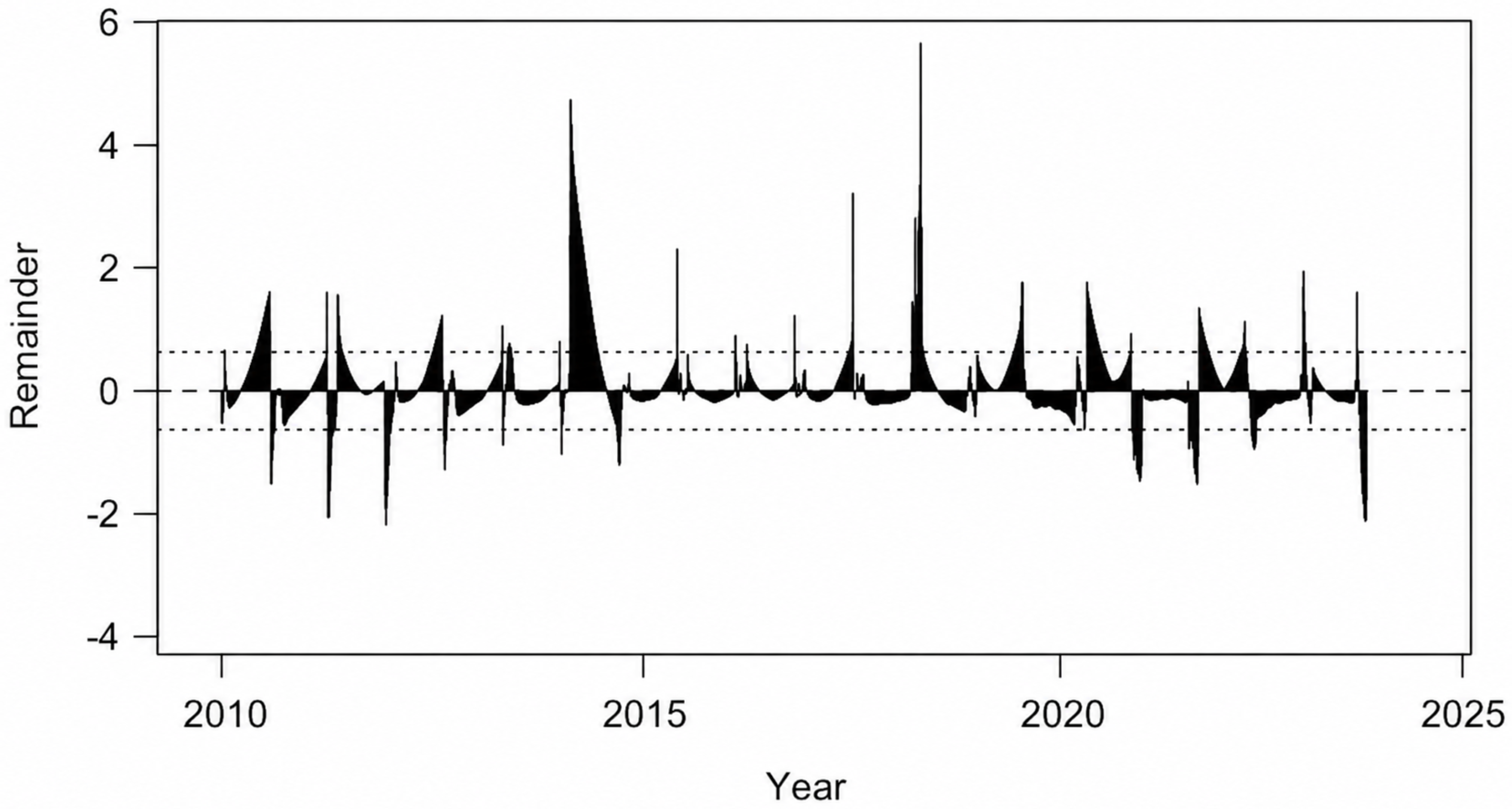
Figure 2 shows the STL remainder component, with the solid horizontal line marking zero and the dotted lines indicating reference limits defined as the residual mean plus or minus two standard deviations. Most residuals fluctuated close to zero and remained within these limits, although several positive and negative excursions crossed the dotted lines. The largest positive spikes occurred during periods when observed ILI activity was substantially higher than the estimated trend-seasonal baseline, while negative spikes indicated activity below the baseline. These exceedances were interpreted as retrospective, baseline-adjusted anomalies rather than prospectively validated outbreak detections.
Figure 2.
STL residuals with residual reference limits .
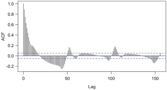
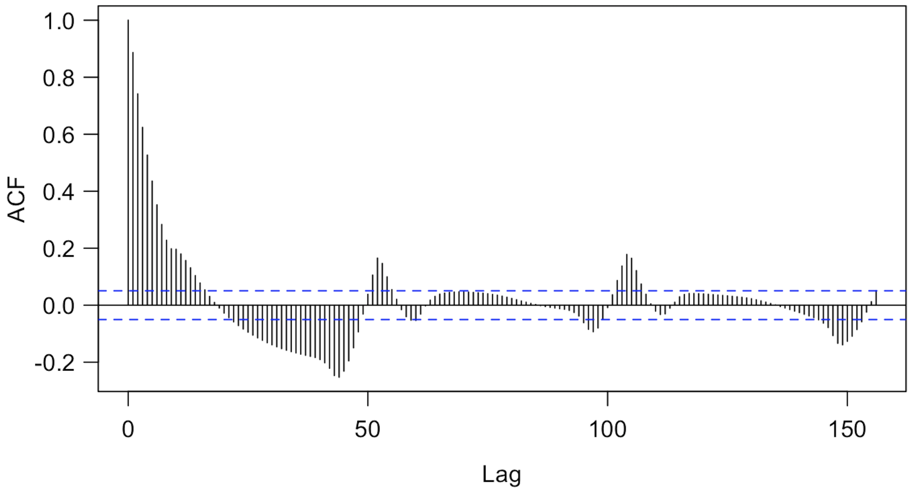
Figure 3 shows the autocorrelation function of the STL residuals, with the blue dashed lines marking the approximate 95% confidence limits expected when residual autocorrelations are close to zero. Bars extending beyond these limits indicate lags where the remaining correlation is larger than would typically be expected from random variation alone. Several autocorrelations exceeded the limits, particularly at short lags, showing that some temporal dependence remained after decomposition. Smaller but noticeable patterns at longer lags also suggested weak residual seasonal structure. Overall, STL removed much of the dominant trend and seasonality, but the residuals should not be treated as independent white noise.
Figure 3.
Autocorrelation function plot of STL residuals.
4.3. Sensitivity of Warning Signals to Threshold Choice
Table 1 summarizes the sensitivity of the retrospective warning signals to the threshold parameter k. For all values of k, the warning rule required two consecutive residual exceedances. Lower values of k produced more warning signals, while higher values produced fewer warning signals. The main rule used in this study, , generated warning signals in four seasons, with an average of 0.20 warning signals per season.
Table 1.
Sensitivity of retrospective warning signals to k.
However, none of the warning signals occurred before the seasonal ILI peak under this retrospective season-level definition. Therefore, mean lead time was not applicable. These results suggest that the two-week persistence rule summarized residual sustain exceedances, but should not be interpreted as a validated prospective early-warning rule.
4.4. SARIMA Benchmark Model Diagnostics
A SARIMA model was fitted to the interpolated weekly ILI series using a seasonal period of 52 weeks. The AICc-selected model was ARIMA(0, 1, 2)(1, 0, 0)52, which includes one nonseasonal difference, two nonseasonal moving-average terms, and one seasonal autoregressive term at the annual weekly period. Table 2 summarizes the model fit statistics and residual diagnostic results.
Table 2.
Diagnostics for the SARIMA benchmark model fitted to weekly national ILI data.
The selected SARIMA model captured part of the regular temporal structure in the weekly ILI series, as reflected by the in-sample error summaries in Table 2. However, the residual diagnostics indicate that some dependence remained after model fitting. In particular, the Ljung–Box test based on 104 lags was statistically significant (, , ), suggesting that the SARIMA residuals were not fully uncorrelated.
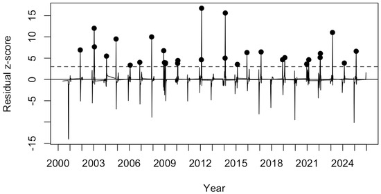
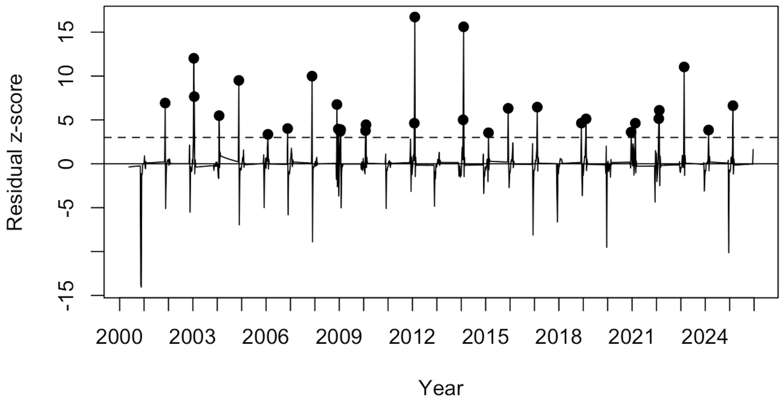
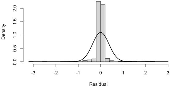
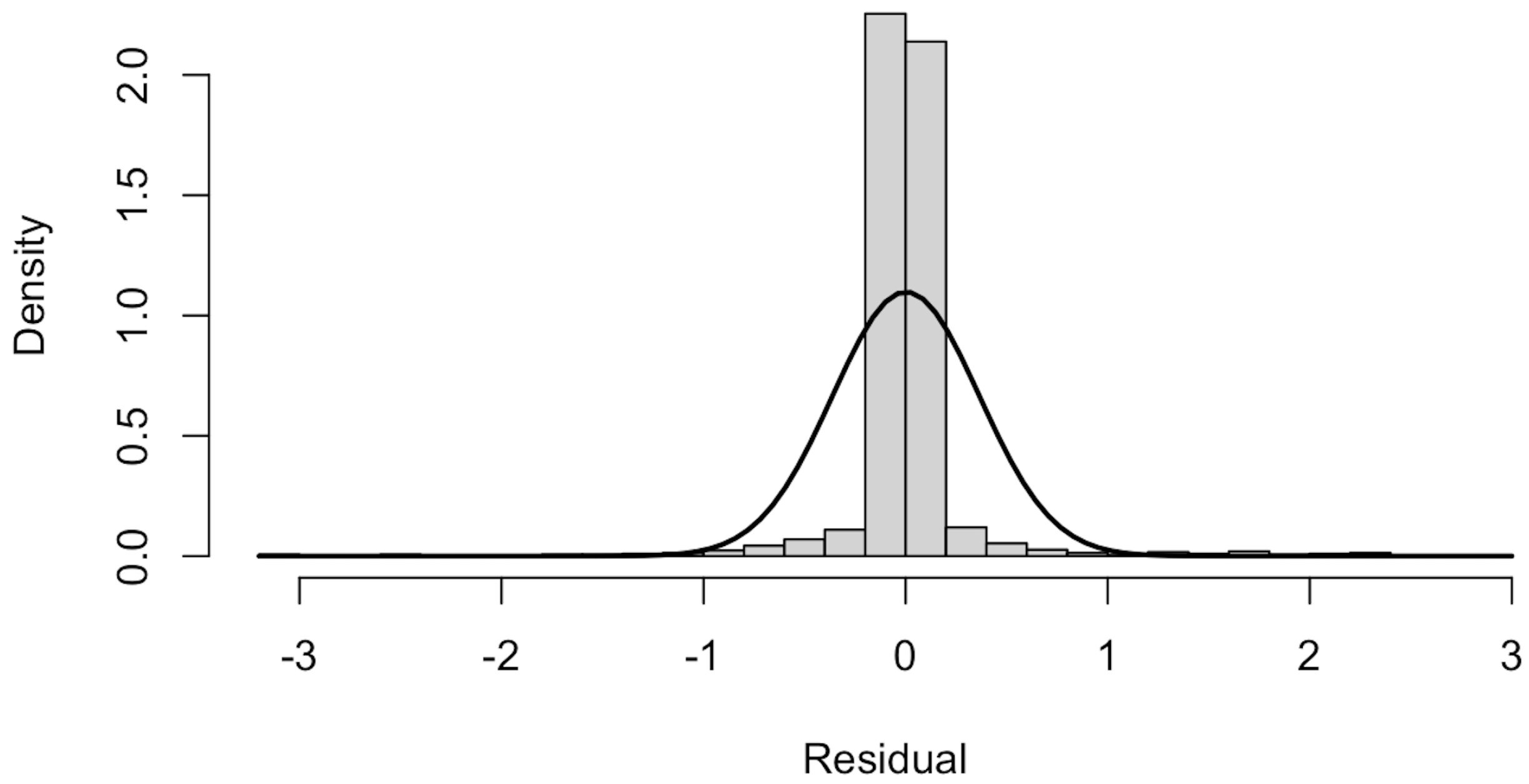
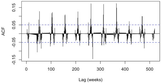
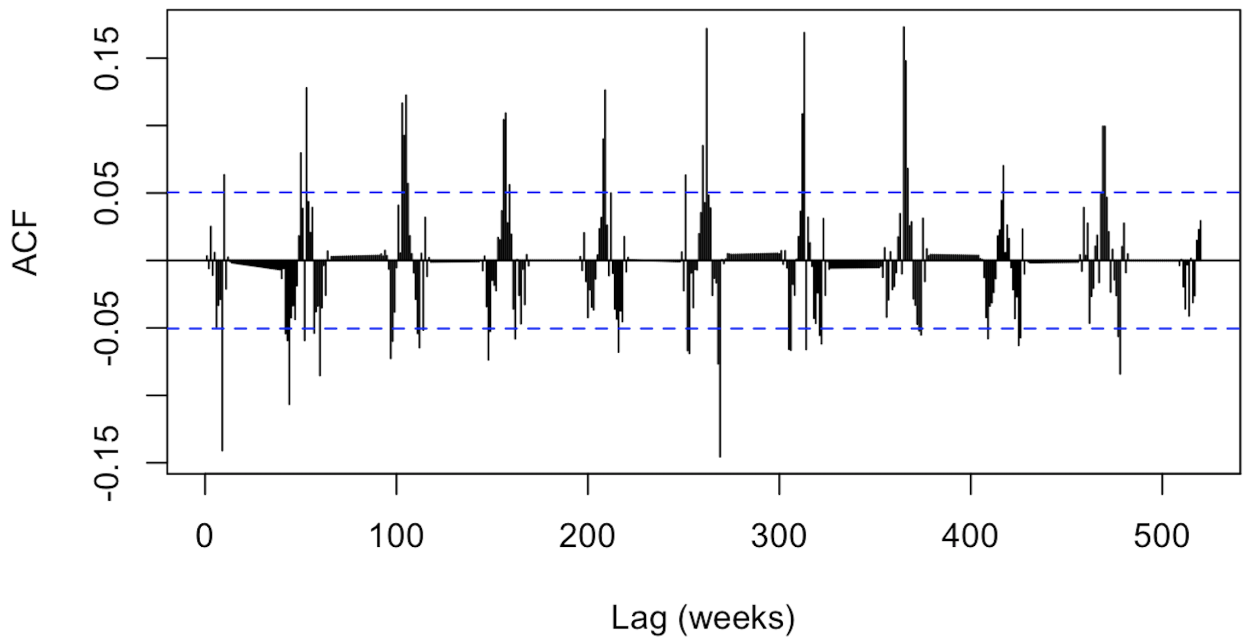
The diagnostic plots provide additional detail on the remaining structure in the SARIMA residuals. Figure 4 shows several large positive and negative residual z-scores. The dotted horizontal lines mark the thresholds used to identify unusually large standardized residuals. Figure 5 shows that the residual distribution is centered near zero but retains visible tail behavior. Figure 6 shows remaining serial dependence at several lags; the blue dashed lines represent approximate 95% confidence limits, and bars extending beyond them indicate autocorrelations larger than expected under white noise. This finding is consistent with the significant Ljung–Box test reported in Table 2. Overall, the SARIMA model provides a useful forecasting benchmark but does not fully remove temporal dependence or atypical deviations from the series.
Figure 4.
Residual z-scores based on a SARIMA model.
Figure 5.
Histogram and density of residuals based on a SARIMA model.
Figure 6.
Autocorrelation function plot of SARIMA residuals.
4.5. Rolling-Origin Forecast Accuracy
Table 3 reports rolling-origin forecast accuracy for the STL-based baseline forecasts, the SARIMA benchmark, the seasonal naive benchmark, and the ETS benchmark at 4-, 8-, and 12-week horizons.
Table 3.
Rolling-origin forecast accuracy of STL-based forecasts and benchmark methods.
For STL and SARIMA, forecast errors generally increased as the forecast horizon became longer. The seasonal naive benchmark showed relatively stable errors across horizons, while the ETS benchmark produced larger errors, especially at the 8- and 12-week horizons. At the 4-week horizon, the STL forecast had the lowest numerical errors among the evaluated methods, with RMSE = 0.925, MAE = 0.546, and MAPE = 22.6%. SARIMA performed similarly at this horizon, with RMSE = 0.929, MAE = 0.568, and MAPE = 25.4%. The seasonal naive benchmark had higher errors at the 4-week horizon, while ETS had the largest errors. At the 8- and 12-week horizons, the seasonal naive benchmark produced the lowest numerical errors. At 8 weeks, seasonal naive had RMSE = 1.270, MAE = 0.758, and MAPE = 36.7%, compared with RMSE = 1.280, MAE = 0.819, and MAPE = 37.3% for STL. At 12 weeks, seasonal naive had RMSE = 1.280, MAE = 0.768, and MAPE = 36.5%, compared with RMSE = 1.450, MAE = 0.957, and MAPE = 46.7% for STL.
These results suggest that the STL-based forecasts were competitive with conventional time-series benchmarks, particularly at the 4-week horizon, but they should not be interpreted as evidence of general forecasting superiority. The practical value of the STL-based baseline is its interpretability and its ability to connect forecasting with the same trend-seasonal baseline used for monitoring and residual interpretation.
5. Discussion
The primary goal of this study was to establish and empirically evaluate a common interpretable baseline for national ILI surveillance, rather than to develop a prospective outbreak-detection system or a generally superior epidemic-forecasting method. The trend, seasonal, and residual components were used to organize monitoring, retrospective anomaly screening, persistence summaries, and short-term baseline forecasting within the same statistical representation. The approach should therefore be viewed as a transparent structure for surveillance interpretation.
These findings are consistent with earlier work showing that decomposition can support the interpretation of surveillance time series. STL was originally developed as a flexible method for separating trend, seasonal, and residual variation [9], and it has previously been applied to syndromic surveillance for modeling, visualization, and disease monitoring [12]. The present study extends this line of work to a long national ILI percentage series and examines several surveillance outputs within the same decomposition. The contribution is therefore not the introduction of STL to disease surveillance, but an empirical illustration of how a single trend–seasonal baseline can connect monitoring, retrospective residual screening, persistence summaries, and short-term reference forecasts.
The forecasting results provide a mixed but informative picture. STL produced the lowest numerical errors at the 4-week horizon, although its performance was very similar to SARIMA. At the 8- and 12-week horizons, the seasonal naive benchmark produced the lowest errors, indicating that annual seasonal recurrence remains a strong reference for medium-term ILI forecasting. One possible interpretation is that the current STL trend contains useful local information at shorter horizons, whereas the previous year’s seasonal trajectory provides a more stable signal as the forecast horizon increases. This explanation is plausible but was not tested directly and should be examined in future work. ETS performed less well in this application, particularly at the longer horizons.
These results do not establish that STL is generally superior to conventional forecasting models. ARIMA and SARIMA models remain widely used because they provide parsimonious representations of temporal dependence and seasonality [7,8], while influenza forecasting studies have demonstrated the value of short-term prediction for operational planning and public-health decision support [13,14]. The practical advantage of the STL approach is different: its forecasts are generated from the same trend–seasonal baseline used to interpret observed activity. This allows expected seasonal progression and baseline-adjusted deviations to be communicated within a common statistical structure.
The residual-screening results should be distinguished from those of established prospective outbreak-detection methods. Farrington-type algorithms and EARS procedures were developed for aberration detection and are typically evaluated using sensitivity, specificity, false-alarm frequency, and timeliness [4,5,6]. Statistical process-control approaches such as CUSUM and EWMA similarly require decision thresholds to be calibrated for operational use [15,16]. In the present study, the residual threshold was used only as a descriptive rule for identifying large positive departures from the estimated STL baseline. Because the residuals retained short-lag autocorrelation, weak seasonal structure, and visible tail behavior, the threshold should not be interpreted as a probability-calibrated control limit or as a formal test of outbreak occurrence.
The persistence analysis reinforces this interpretation. Increasing the threshold parameter k reduced the frequency of persistence signals, but none of the two-week signals occurred before the seasonal ILI peak under the season-level definition used in this study. The rule therefore summarized sustained atypical activity after adjustment for the trend and seasonal baseline, but it did not provide meaningful pre-peak warning. Prospective use would require thresholds to be estimated using only information available at the time of analysis and calibrated against clearly defined public-health targets. It would also require formal evaluation of sensitivity, specificity, false-alarm frequency, and lead time.
The role of this approach is also distinct from that of modern ensemble forecasting systems. Collaborative influenza forecasting studies have shown that combining models can improve prospective prediction and reduce dependence on any single modeling assumption [14]. Similar benefits have been reported for ensemble forecasts in other infectious-disease settings [17,18]. STL is not intended to replace these systems. Instead, it may serve as a simple and interpretable reference layer against which statistical, mechanistic, or ensemble forecasts can be compared. In particular, the decomposition can help clarify whether an observed or forecasted increase reflects expected seasonal progression or a departure from the estimated baseline.
Several limitations should be considered. First, the analysis used national aggregate ILI data, which may conceal regional differences in epidemic timing, intensity, and reporting. Second, ILI is a syndromic measure rather than a laboratory-confirmed influenza outcome and may reflect other respiratory infections, changes in healthcare-seeking behavior, or changes in surveillance participation. Long-term changes in the estimated trend may therefore reflect both disease activity and changes in the surveillance system.
Third, the residual-screening and persistence analyses were retrospective, and the STL decomposition used for these summaries was fitted to the full study period. The resulting residual exceedances should consequently be interpreted as historical baseline-adjusted summaries rather than as real-time detections. The threshold was selected as a simple descriptive rule and was not prospectively optimized or calibrated. Fourth, missing values were linearly interpolated for analyses requiring a complete regular time series. Although interpolated observations were not used as validation outcomes or counted as observed anomaly events, interpolation may still have influenced the estimated components and forecasts. Finally, the fixed 52-week seasonal period approximates the epidemiological calendar and treats week 53 as part of the continuous weekly sequence.
In practice, an STL baseline would be most useful when considered alongside other surveillance indicators, such as virological testing, hospitalization data, regional ILI patterns, and mechanistic or ensemble forecasts. Future work should evaluate the framework at regional and state levels under real-time or pseudo-prospective conditions, while exploring alternative seasonal specifications, missing-data methods, and calibrated residual thresholds. Further research should also assess probabilistic forecasts and clarify why STL performed best at 4 weeks while seasonal naive performed better at longer horizons. Hybrid machine-learning or deep-learning models could build on the STL components or residuals to capture more complex patterns while preserving interpretability.
6. Conclusions
Using weekly national U.S. ILI data, this study evaluated whether STL decomposition could provide a common and interpretable baseline for monitoring, retrospective residual screening, and short-term forecasting. The trend and seasonal components represented expected ILI activity, while the residual component summarized deviations from that expectation. STL produced the lowest numerical forecast errors at the 4-week horizon, although its performance was nearly identical to that of SARIMA, while the seasonal naive method produced the lowest errors at the 8- and 12-week horizons.
The empirical results support STL primarily as a transparent organizing baseline rather than as a validated alerting system or a generally superior forecasting model. The tested persistence rule produced no pre-peak signals, and the retrospective residual thresholds would require prospective calibration before operational use. Within these limitations, STL provides an interpretable reference for distinguishing expected seasonal progression from baseline-adjusted deviations and for connecting surveillance monitoring with short-term forecasting.
Author Contributions
Conceptualization, C.M. and Z.X.; methodology, C.M. and Z.X.; formal analysis, C.M.; writing—original draft preparation, C.M.; writing—review and editing, C.M. and Z.X. All authors have read and agreed to the published version of the manuscript.
Funding
This research received no external funding.
Institutional Review Board Statement
Not applicable.
Informed Consent Statement
Not applicable.
Data Availability Statement
Publicly available data were used in this study. The data are available from the U.S. Centers for Disease Control and Prevention FluView/ILINet platform.
Acknowledgments
The authors thank John Musgrave for his valuable suggestions and for his assistance with English-language editing, and Jiaxi Lin for carefully proofreading the manuscript. The authors also thank the U.S. Centers for Disease Control and Prevention for providing access to national influenza-like illness surveillance data through ILINet and FluView.
Conflicts of Interest
The authors declare no conflict of interest.
References
- Centers for Disease Control and Prevention. FluView Interactive: National, Regional, and State Level Outpatient Illness and Viral Surveillance. Available online: https://gis.cdc.gov/grasp/fluview/fluportaldashboard.html (accessed on 21 December 2025).
- Thompson, W.W.; Moore, M.R.; Weintraub, E.; Cheng, P.Y.; Jin, X.; Bridges, C.B.; Bresee, J.S.; Shay, D.K. Estimating influenza-associated deaths in the United States. Am. J. Public Health 2009, 99, S225–S230. [Google Scholar] [CrossRef] [Scilit] [PubMed]
- Serfling, R.E. Methods for current statistical analysis of excess pneumonia-influenza deaths. Public Health Rep. 1963, 78, 494–506. [Google Scholar] [CrossRef] [Scilit] [PubMed]
- Farrington, C.P.; Andrews, N.J.; Beale, A.D.; Catchpole, M.A. A statistical algorithm for the early detection of outbreaks of infectious disease. J. R. Stat. Soc. Ser. A 1996, 159, 547–563. [Google Scholar] [CrossRef] [Scilit]
- Hutwagner, L.; Thompson, W.W.; Seeman, G.M.; Treadwell, T. An algorithm for detecting influenza epidemics. Am. J. Public Health 2003, 93, 2030–2036. [Google Scholar]
- Hutwagner, L.; Thompson, W.W.; Seeman, G.M.; Treadwell, T. The bioterrorism preparedness and response Early Aberration Reporting System (EARS). J. Urban Health 2005, 82, i89–i96. [Google Scholar]
- Box, G.E.P.; Jenkins, G.M. Time Series Analysis: Forecasting and Control; Holden-Day: San Francisco, CA, USA, 1976. [Google Scholar]
- Hyndman, R.J.; Athanasopoulos, G. Forecasting: Principles and Practice; OTexts: Melbourne, Australia, 2018. [Google Scholar]
- Cleveland, R.B.; Cleveland, W.S.; McRae, J.E.; Terpenning, I. STL: A Seasonal-Trend Decomposition Procedure Based on Loess. J. Off. Stat. 1990, 6, 3–73. [Google Scholar]
- Akaike, H. A new look at the statistical model identification. IEEE Trans. Autom. Control 1974, 19, 716–723. [Google Scholar] [CrossRef] [Scilit]
- Ljung, G.M.; Box, G.E.P. On a measure of lack of fit in time series models. Biometrika 1978, 65, 297–303. [Google Scholar] [CrossRef]
- Hafen, R.P.; Anderson, D.E.; Cleveland, W.S.; Maciejewski, R.; Ebert, D.S.; Abusalah, A.; Yakout, M.; Ouzzani, M.; Grannis, S.J. Syndromic Surveillance: STL for Modeling, Visualizing, and Monitoring Disease Counts. BMC Med. Inform. Decis. Mak. 2009, 9, 21. [Google Scholar] [CrossRef] [Scilit] [PubMed]
- Shaman, J.; Karspeck, A. Forecasting seasonal outbreaks of influenza. Proc. Natl. Acad. Sci. USA 2012, 109, 20425–20430. [Google Scholar] [CrossRef] [Scilit] [PubMed]
- Reich, N.G.; Brooks, L.C.; Fox, S.J.; Kandula, S.; McGowan, C.J.; Moore, E.; Osthus, D.; Ray, E.L.; Tushar, A.; Yamana, T.K.; et al. A collaborative multiyear, multimodel assessment of seasonal influenza forecasting in the United States. Proc. Natl. Acad. Sci. USA 2019, 116, 3146–3154. [Google Scholar] [CrossRef] [Scilit] [PubMed]
- Fricker, R.D. Introduction to statistical methods for biosurveillance. Wiley Interdiscip. Rev. Comput. Stat. 2013, 5, 252–260. [Google Scholar]
- Montgomery, D.C. Introduction to Statistical Quality Control; Wiley: Hoboken, NJ, USA, 2009. [Google Scholar]
- Brooks, L.C.; Ray, E.L.; Bien, J.; Biggerstaff, M.; Bosse, N.I.; Bracher, J.; Cramer, E.Y.; Funk, S.; Gerding, A.; Johansson, M.A.; et al. Comparing ensemble approaches for short-term probabilistic COVID-19 forecasts in the United States. Proc. Natl. Acad. Sci. USA 2020, 117, 29935–29942. [Google Scholar]
- Yamana, T.K.; Kandula, S.; Shaman, J. Superensemble forecasts of dengue outbreaks. J. R. Soc. Interface 2017, 14, 20170210. [Google Scholar]

Disclaimer/Publisher’s Note: The statements, opinions and data contained in all publications are solely those of the individual author(s) and contributor(s) and not of MDPI and/or the editor(s). MDPI and/or the editor(s) disclaim responsibility for any injury to people or property resulting from any ideas, methods, instructions or products referred to in the content. |
© 2026 by the authors. Licensee MDPI, Basel, Switzerland. This article is an open access article distributed under the terms and conditions of the Creative Commons Attribution (CC BY) license.