BSTZINB: A Bayesian Framework for Negative-Binomial Modeling of Spatio-Temporal Zero-Inflated Count Data in Epidemiology

Abstract

Modern Bayesian hierarchical methodologies allow us to leverage spatio-temporal dependencies between observations, enhancing both health effect estimation and map visualization in efficient and flexible ways. However, the necessary levels of statistical software are often unavailable or difficult to access. We have recently examined Bayesian spatio-temporal models to estimate the association between COVID-19 death counts and various social and environmental risk factors, including ambient air pollution exposure. Typically, it is very common that in an infection disease mapping problem with count data, we have excessive zeros, and it is usually for over-dispersed count outcome variables. Furthermore, the theory suggests that the excess zeros are generated by a separate process from the count values and that the excess zeros need to be modeled independently. Our proposed models are specially designed to handle the zero-inflation and over-dispersion in count data through Zero-Inflated Negative Binomial regression with random effects that vary across time and space within a Markov Chain Monte Carlo framework. Drawing on our knowledge and experience, we aim to provide a simple, unified, and publicly available software that can be applied in various disease mapping studies under the contemporary Bayesian framework.

1. Introduction

This paper introduces a new R package, BSTZINB (available through CRAN https://cran.r-project.org/web/packages/BSTZINB/index.html, accessed on 13 July 2026), for statistical modeling and inference with various Bayesian spatio-temporal models specially designed for zero-inflated count data [1]. We are strongly motivated by recent catastrophic world events like the COVID-19 pandemic. In any infectious disease, the number of infected cases and related deaths vary spatially and temporally as the disease spreads over time and adjacent regions. In addition, the spread of the disease and the related degree of severity of the health outcomes can be heavily affected by several biological, socioeconomic, and environmental factors [2,3,4]. For example, in a recently published study on modeling the COVID-19 pandemic, we found evidence that long-term exposure to air pollution might have increased the severity of COVID-19 weekly death counts in the early period of the pandemic in the United States [1].

The problem of zero-inflation arises when the large numbers of zeros in count data cannot be accommodated properly by a standard discrete distribution like the Poisson or Negative Binomial distribution [5,6,7]. When count data contain an unusually large proportion of zero observations, often referred to as “excess zeros,” standard Poisson and even conventional Negative Binomial models may inadequately capture the observed frequency of zeros, resulting in poor model fit and biased inference [5,8]. In addition, the non-zero observations frequently exhibit over-dispersion relative to the Poisson distribution, which can lead to biased parameter estimates, underestimated standard errors, and inflated Type I error rates when ignored [9,10]. In count-data applications, over-dispersion occurs when the conditional variance exceeds the conditional mean, thereby violating the equidispersion assumption of the Poisson model [9,10].

Bayesian modeling has emerged as a very popular tool for analyzing spatio-temporal data due to its flexibility in incorporating prior information, modeling complex dependency structures, and handling zero-inflation and over-dispersion cases, which are common in epidemiological studies [11,12,13,14]. There is an enormous need, especially among epidemiologists, for simple, unified, and publicly available software for such modern epidemiological research [11,14,15]. In that respect, [16] provides a related Bayesian zero-inflated Negative Binomial framework for spatio-temporal count data, which is methodologically relevant to the present manuscript. However, their [16] software is not distributed as a standard R package through CRAN and therefore does not provide the same level of direct accessibility, installation, documentation, and integration into routine R workflows.

Bayesian hierarchical models have become increasingly popular in epidemiological research because they can simultaneously accommodate over-dispersion, excess zeros, spatial correlation, temporal dependence, and uncertainty quantification within a unified inferential framework [1,17]. Such models have been successfully used to study disease incidence, mortality, and environmental health outcomes observed across geographic regions and over time. Our BSTZINB package translates these methodological advances into an accessible software tool, enabling researchers to fit a broad class of Bayesian count-data models without requiring extensive expertise in Bayesian computation. Specifically, the package implements Bayesian Negative Binomial (BNB), Bayesian Zero-Inflated Negative Binomial (BZINB), Bayesian Spatio-Temporal Negative Binomial (BSTNB), and Bayesian Spatio-Temporal Zero-Inflated Negative Binomial (BSTZINB) models using efficient Markov Chain Monte Carlo (MCMC) algorithms, while also providing tools for model assessment, visualization, disease mapping, and statistical reporting.

The BSTZINB package provides a suite of tools for data description, Bayesian modeling, and result summaries for spatio-temporal health outcomes. It is developed with the understanding that the end-user may not be an expert in Bayesian statistics or spatio-temporal modeling. Therefore, special care is provided for the package to communicate the model-based “knowledge discovery” to the end-user. In summary, this package offers a broad range of models, including (a) BNB—a Bayesian Negative Binomial model; (b) BZINB—a Bayesian Zero-Inflated Negative Binomial model; (c) BSTNB—a Bayesian Spatiotemporal Negative Binomial model; and (d) BSTZINB—a Bayesian Spatiotemporal Zero-Inflated Negative Binomial model. To our knowledge, no other package offers similar user-friendly Bayesian modeling for zero-inflated spatio-temporal epidemiology data like our BSTZINB package, complete with both inferential and visualization tools. In our BSTZINB package, we have carefully optimized the MCMC procedure to enhance speed and ensure efficient, tractable inference for all models within a reasonable computation time. This optimization supports practical implementation in real data analysis settings, especially for general practitioners who may not be experts in Bayesian MCMC-based model fitting methods.

The rest of the paper is organized as follows: in Section 2, we provide a brief background knowledge on different types of count data, zero-inflated, and over-dispersed models. In Section 3, we describe the general application of our software and how an end-user can effortlessly use our package. Section 4 provides a walk-through example, including each step from data input to inference. It covers the entire process: starting with data input, then setting up (prior distribution and MCMC parameter choices), and running the model fitting. It continues with post-processing of the model outputs, diagnostics, and inference of the model or its parameters. Section 5 concludes the paper with a general helpful discussion of our findings and suggestions for possible future extensions. In the Supplementary Materials document we have provided additional simulation studies, benchmarking with other competing methods/packages, and MCMC convergence diagnostics and studies.

2. Methods

Depending on a spatio-temporal dependency and a zero-inflated nature of data, we can construct a Bayesian spatio-temporal model that assumes either standard or spatio-temporal (ST), with or without a Zero-Inflated (ZI) model component. We now provide a generic model structure that covers nested sub-models in the following illustration.

Suppose that we observe $k=1,\dots ,n$ samples, and each of them is assigned to the ith region (e.g., county) at time j. Let us consider the following data model equation [17]:

$$y_{ij}\sim \left(1-q_{ij}\right){\mathbb{1}}_{\left({\mathrm{w}}_{ij}=0\wedge y_{ij}=0\right)}+q_{ij}\mathrm{NB}\left(p_{ij},r\right){\mathbb{1}}_{\left({\mathrm{w}}_{ij}=1\right)},$$

(1)

where y represents a disease count, and q represents the probability at risk of exposure that follows a Negative Binomial risk distribution, denoted as $\mathrm{NB}$. The probability of contracting the disease among the individuals in the exposed population is given by p and the mean-variance dispersion parameter is given by r. A random variable w is a binary label with the disease at-risk probability q, and ∧ is a symbol of logical conjunction. ${\mathbb{1}}_{(·)}$ is a zero-one indicator made from the condition in the subscript condition. Now, we introduce the following model structures according to the way of modeling p and q. Note that in Equation (1), k indexes the observation-level record, while $(i,j)$ indexes the corresponding spatial unit and time point.

2.1. Bayesian Zero-Inflated Negative Binomial Model (BZINB)

If an outcome is independent of both space and time, then we do not need to specify the space-time structure of the equation, so that the generic model (1) can be simplified into $y_k\sim \left(1-q_k\right){\mathbb{1}}_{\left({\mathrm{w}}_k=0\wedge y_k=0\right)}+q_k\mathrm{NB}\left(p_k,r\right){\mathbb{1}}_{\left({\mathrm{w}}_k=1\right)}$. Consequently, we model $q_k$ and $p_k$ as,

$$logit\left(q_k\right)={\beta }_{10}+{\displaystyle \sum _{d=1}^{D_1}}{\beta }_{1d}{X}_{kd},$$

(2)

$$logit\left(p_k\right)={\beta }_{20}+{\displaystyle \sum _{d=1}^{D_2}}{\beta }_{2d}{X}_{kd},$$

(3)

where ${\beta }_{1d}$ represents the coefficient of the fixed effect covariates (${\beta }_{11},\cdots ,{\beta }_{1D_1})$ as well as an intercept (${\beta }_{10}$) in the q-model component for probability-at-risk, while ${\beta }_{2d}$ represents the same but in the p-model component for at-risk population. Here, $D_1$ denotes the number of covariates included in the at-risk or zero-inflation component, while $D_2$ denotes the number of covariates included in the Negative Binomial count component. Note that the two sets of covariates may be identical, partially overlapping, or different depending on the scientific question. If the same covariates are used in both components, the model allows the same predictors to have potentially different effects on the probability of being at risk and on the count intensity among at-risk observations. If different covariates are used, the user can model separate mechanisms for structural zeros and positive counts.

2.2. Bayesian Spatio-Temporal Negative Binomial Model (BSTNB)

If we do not consider excessive zero counts, then we only need to specify a model for $p_{ij}$, since $q_{ij}\equiv 1$ in Equation (1). Thus, we assume $y_{ij}\sim \mathrm{NB}\left(p_{ij},r\right)$ and consider

$$logit\left(p_{ij}\right)={\beta }_0+{\displaystyle \sum _{d=1}^D}{\beta }_d{X}_d+{\displaystyle \sum _{m=1}^M}{\beta }_{(D+m)}{T}_m+b_{i1}+b_{i2}{t}_{ij},$$

(4)

where this model further requires the definition of a basis function T and a random coefficient b. Given the number of basis functions, m, $T_1,\cdots ,T_m$ are determined by principles of cubic B-spine basis functions [18]. This is used to capture the non-linear fixed time effect. $b_{i1}$ refers to a random intercept within the ith region, while $b_{i2}$ refers to a random slope along the time points $t_{ij}$ within the ith region. These are used to capture random effects of space and time, which might interact with each other. The cubic B-spline basis provides sufficient flexibility to capture nonlinear temporal patterns, such as peaks, plateaus, and changing rates of increase or decrease over time. Consequently, the spline representation allows the model to describe complex temporal dynamics commonly observed in epidemiological count data while maintaining smoothness and computational stability. The random effects $b_{i1}$ and $b_{i2}$ further allow each spatial region to have its own intercept and temporal trajectory around this overall population-level trend.

2.3. Bayesian Spatio-Temporal Zero-Inflated Negative Binomial Model (BSTZINB)

Following Equation (1), we model q and p as,

$$logit\left(q_{ij}\right)={\beta }_{10}+{\displaystyle \sum _{d=1}^{D_1}}{\beta }_{1d}{X}_d+{\displaystyle \sum _{m=1}^M}{\beta }_{1(D_1+m)}{T}_m+b_{1i1}+b_{1i2}{t}_{ij},$$

(5)

$$logit\left(p_{ij}\right)={\beta }_{20}+{\displaystyle \sum _{d=1}^{D_2}}{\beta }_{2d}{X}_d+{\displaystyle \sum _{m=1}^M}{\beta }_{2(D_2+m)}{T}_m+b_{2i1}+b_{2i2}{t}_{ij},$$

(6)

where ${\mathit{b}}_{1i}={\left(b_{1i1},b_{1i2}\right)}^T$ and ${\mathit{b}}_{2i}={\left(b_{2i1},b_{2i2}\right)}^T$ represent the random effects corresponding to $q_{ij}$ and $p_{ij}$, respectively. We impose a multivariate ICAR prior structure [1] on ${\mathit{\varphi }}_i={\left({\mathit{b}}_{1i}^T,{\mathit{b}}_{2i}^T\right)}^T$ as,

$${\mathit{\varphi }}_i\mid {\mathit{\varphi }}_{(-i)},\mathbf{\Gamma }\sim {\mathrm{N}}_4\left({\displaystyle \frac{1}{m_i}}\sum _{l\in {\partial }_i}{\mathit{\varphi }}_l,{\displaystyle \frac{1}{m_i}}\mathbf{\Gamma }\right),$$

(7)

where $\mathbf{\Gamma }/m_i$ is a $4\times 4$ unknown conditional covariance matrix and is estimated through the MCMC algorithm. This multivariate ICAR allows spatial dependence and region-specific random time trends within count components and excess-zero components as well as dependence between them. This model will be referred to as BSTZINB-NLT in the rest of the paper, where NLT refers to the non-linear fixed time trend for q.

We hypothesize that the assumption of a non-linear fixed time trend for q might not be necessary in some cases due to model parsimony. Thus, we further assume a linear time-fixed trend for q, i.e., ${\beta }_{1(D_1+1)}={\beta }_{1(D_1+2)}=\cdots ={\beta }_{1(D_1+M)}=0$. In other words, we consider

$$logit\left(q_{ij}\right)={\beta }_{10}+{\displaystyle \sum _{d=1}^{D_1}}{\beta }_{1d}{Z}_d+b_{1i1}+b_{1i2}{t}_{ij}.$$

(8)

This model will be referred to as BSTZINB-LT in the rest of the paper, where LT refers to a linear fixed time trend for q.

Conditional posterior sampling algorithms are mostly adopted from [1], and it is straightforward to implement our algorithms to all the illustrated approaches. For instance, we draw an at-risk indicator $w_{ij}$ from a Bernoulli distribution with ${\eta }_{ij}={\displaystyle \frac{q_{ij}^r(1-p_{ij})}{q_{ij}^r(1-p_{ij})+p_{ij}}}$, where $q_{ij}$ and $p_{ij}$ were defined in Section 2.3 for zero-inflated models, while we always draw $w=1$ for every iteration in practice for the non Zero-Inflated models. To update ${\mathit{\beta }}_1$, we draw a latent variable ${\xi }_{1ij}$ from a Pólya-Gamma distribution $PG(1,{\eta }_{1ij})$, as shown in [19]. Given $\mathit{w}$ and ${\mathit{\xi }}_1$, the full conditional distribution of ${\mathit{\beta }}_1$ is

$$\begin{array}{c}\hfill Pr\left({\mathit{\beta }}_1|\mathit{w},{\mathit{\xi }}_1\right)\propto \pi \left({\mathit{\beta }}_1\right)exp\left[-{\displaystyle \frac{1}{2}}{({\mathit{z}}_1-\mathit{X}{\mathit{\beta }}_1)}^T{\Omega }_1({\mathit{z}}_1-\mathit{X}{\mathit{\beta }}_1)\right],\end{array}$$

(9)

where $\mathit{X}$ is a $n\times p$ design matrix, $\pi \left({\mathit{\beta }}_1\right)$ is the prior distribution $N_p\left({\beta }_0,{\Sigma }_0\right)$, ${\mathit{z}}_1=(\mathit{w}-1/2)/{\mathit{\xi }}_1$, and ${\Omega }_1$ is a $n\times n$ precision matrix, $diag\left({\mathit{\xi }}_1\right)$. Therefore, we update ${\mathit{\beta }}_1$ from $N_p\left(\mu ,\Sigma \right)$ where $\Sigma ={\left({\Sigma }_0^{-1}+X^T{\Omega }_{1}X\right)}^{-1}$ and $\mu =\Sigma \left({\Sigma }_0^{-1}{\beta }_0+X^T{\Omega }_1{\mathit{z}}_1\right)$ with given ${\mathit{z}}_1$. We update ${\mathit{\beta }}_2$ by a similar process using the corresponding Pólya-Gamma distribution $PG(y_{ij}+r,{\eta }_{2ij})$ as discussed in [1,17,20].

3. Software Description

To use our BSTZINB R-package (≥3.5) we need datasets that include a response variable as a count variable of interest (e.g., disease counts), covariates (e.g., risk factors), spatial coordinates, and time points. Also, spatial map information, such as the shape of the areal units and the adjacency information among the areal units, is necessary.

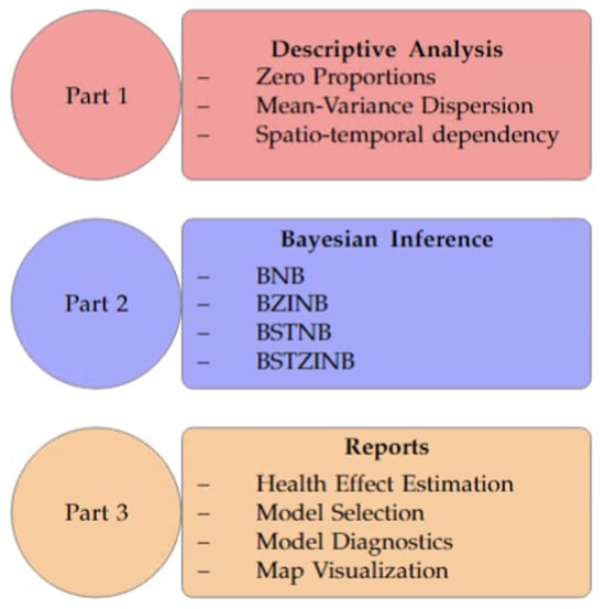
For the descriptive analysis (Part 1) Figure 1, the BSTZINB R-package reshapes original data for model fitting and constructs the adjacency matrix to account for spatial dependency. After that, it can provide conventional summary statistics, including histograms and informative statistics, such as Moran’s I [21,22]. Moran’s I is used as an exploratory diagnostic to assess whether neighboring spatial units tend to have similar outcome values. A significant positive Moran’s I provides empirical motivation for including spatially structured random effects in the Bayesian model. We can investigate whether the response variable has either significant spatio-temporal dependency or a high proportion of zero rates so that our spatio-temporal zero-inflated hierarchical modeling may improve the model fitting compared to the conventional ones.

Figure 1. A flow chart of the BSTZINB R-package: Part 1. Descriptive analysis—we explore the data to determine the most effective statistical methods; Part 2. Bayesian inference—we give a solution to apply several Bayesian models such as Bayesian Zero-Inflated Negative Binomial (BZINB), Bayesian Spatio-Temporal Negative Binomial (BSTNB), and Bayesian Spatio-Temporal Negative Zero-Inflated Negative Binomial (BSTZINB); Part 3. Reports—we provide various solutions to health effect estimation, model selection, model diagnostics, and map visualizations for an epidemiological study.

For the primary modeling (Part 2) Figure 1, the BSTZINB R-package provides Bayesian Negative Binomial regression model solutions: BNB, BZINB, BSTNB, and BSTZINB. In Table 1 we provide a comprehensive list of all available functions in our BSTZINB R-package and their short description.

Table 1. Summary of functions in the BSTZINB package.

Function	Descriptions
BNB	Fit a Bayesian Negative Binomial model
BZINB	Fit a Bayesian Zero-Inflated Negative Binomial model
BSTNB	Fit a Bayesian Spatio-Temporal Negative Binomial model
BSTZINB	Fit a Bayesian Spatio-Temporal Zero Inflated Negative Binomial model
USDmapCount	Produce a disease map over the counties in the US
get_adj_mat	Provide the adjacency matrix for the study counties
qRankPar	Produce a descending order of bar plot for time-averaged log-q estimates over quantile-representative counties
qRankParTop	Produce a descending order of bar plot for time-averaged log-q estimates over the top ranking counties
TimetrendCurve	Produce a time-trend curve over the study time domain for a county
ResultTableSummary	Produce a concise summary table for a model fit
ResultTableSummary2	Produce a full result summary table for all the model-fit objects
compute_ZINB_DIC	Compute a DIC for a zero-inflated Negative Binomial model-fit object
compute_NB_DIC	Compute a DIC for a standard Negative Binomial model-fit object
conv.test	Provide test results of MCMC convergence for specific model-fit object

In our BSTZINB package, the four Bayesian Negative-Binomial regression models (BNB, BZINB, BSTNB, and BSTZINB) require input variables such as a spatio-temporally indexed response variable (y), covariates (X), and a spatial-unit adjacency matrix (A). Our package allows for the choice of a linear/nonlinear temporal structure for the at-risk probability modeling (LinearT), and the various Bayesian MCMC parameter settings, such as the number of MCMC chains (nchain), the number of iterations (niter), the number of burn-in samples (nburn), and the number of thinning samples (nthin) [23].

The BSTZINB model outcome provides MCMC samples of coefficients for the fixed effect covariates in the structural zero model component (alpha) and in the negative-binomial model component (beta). It also includes MCMC samples of the dispersion parameter. These MCMC samples are obtained by a random-walk Metropolis–Hastings update [17] (R) and by two-stage Gibbs update [24] (R2). The MCMC samples of the conditional covariance coefficients (Sigphi) and country-specific random effects (PHI1,PHI2,PHI3,PHI4), the MCMC samples for logit of the estimated probability at risk (eta1), logit of the Negative Binomial probability (eta2) and at-risk indicators (I) are also provided as model outputs for downstream statistical inference and estimation. BSTNB and BNB are similar functions but do not consider zero-inflated modeling. It requires the same input variables as BSTZINB, and there are no outcomes for the structural zero model component, such as alpha, PHI1, PHI2, Eta2, by definition. Appendix A includes brief backgrounds of Bayesian Inference and methodological illustrations for interested readers.

For the model outputs (Part 3), our package provides various model-fitting results and plots focusing on spatial and temporal effect estimation within the Bayesian MCMC regression framework. Appendix B illustrates specific arguments and output of this package’s main (Appendix B.2) and auxiliary functions (Appendix B.3), as well as imports and suggests of libraries (Appendix B.4). In the next section, we present one vignette with a simulated data set.

4. An Illustrative Example

In this section, we provide a step-by-step guide on how to use our BSTZINB R package with the help of a synthetic data set.

4.1. Installing BSTZINB Package

The BSTZINB package is available on CRAN and is ready to be installed and used by the user. The easiest way to install the package is running the following command in the R Console:

Once the BSTZINB package is installed, it can be loaded like any other R packages:  

After the library BSTZINB is loaded, all warning messages as listed above can be ignored as they have no bearing in running our models.

4.2. A Toy Data Set for Step-by-Step Demonstration

We created a synthetic data set that resembles a typical zero-inflated count data over space and time that we often see in many epidemiological studies.

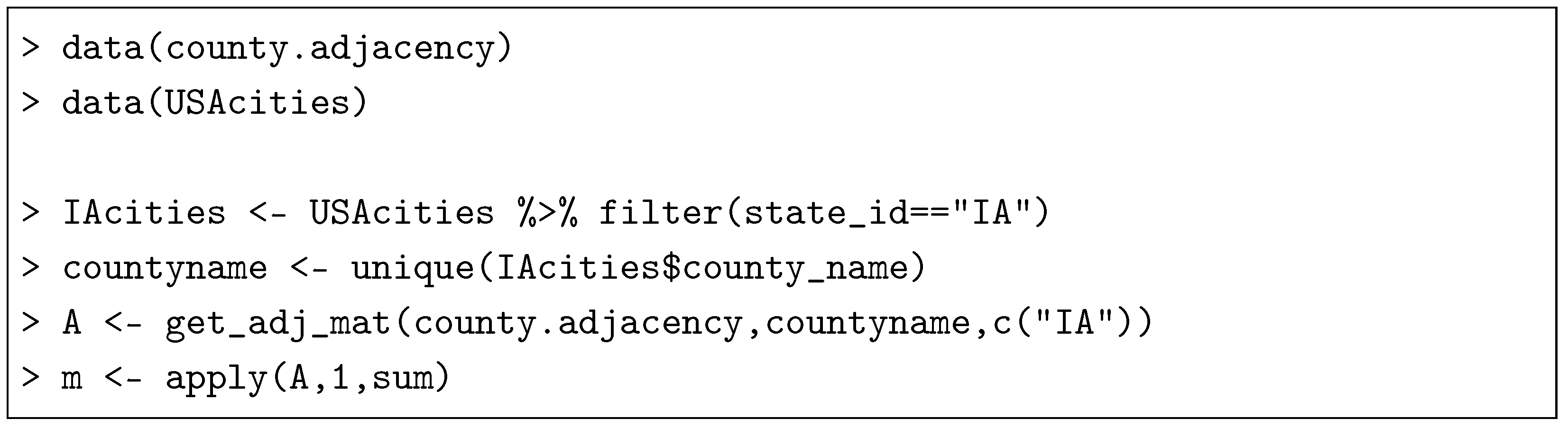
The BSTZINB package utilizes user-supplied geospatial map information and creates toy adjacency information of the areal units in this simulated study domain. In this example, we use the counties from the state of Iowa in the United States to create a spatial adjacency matrix A. We import the county name and the adjacency information from the US census data made in 2010 (available in the package as county.adjacency and USAcities; See Appendix B.1), and one of our functions, get_adj_mat, transform that information into an adjacency matrix A for the counties of our interest. Thereafter, we consider 16 evenly spaced time points across 99 spatial units, which correspond to all the counties in the state of Iowa. Consequently, the complete dataset has 1584 observations with four variables, including county index(sid), time index(tid), outcome disease counts (y), and a covariate (x).

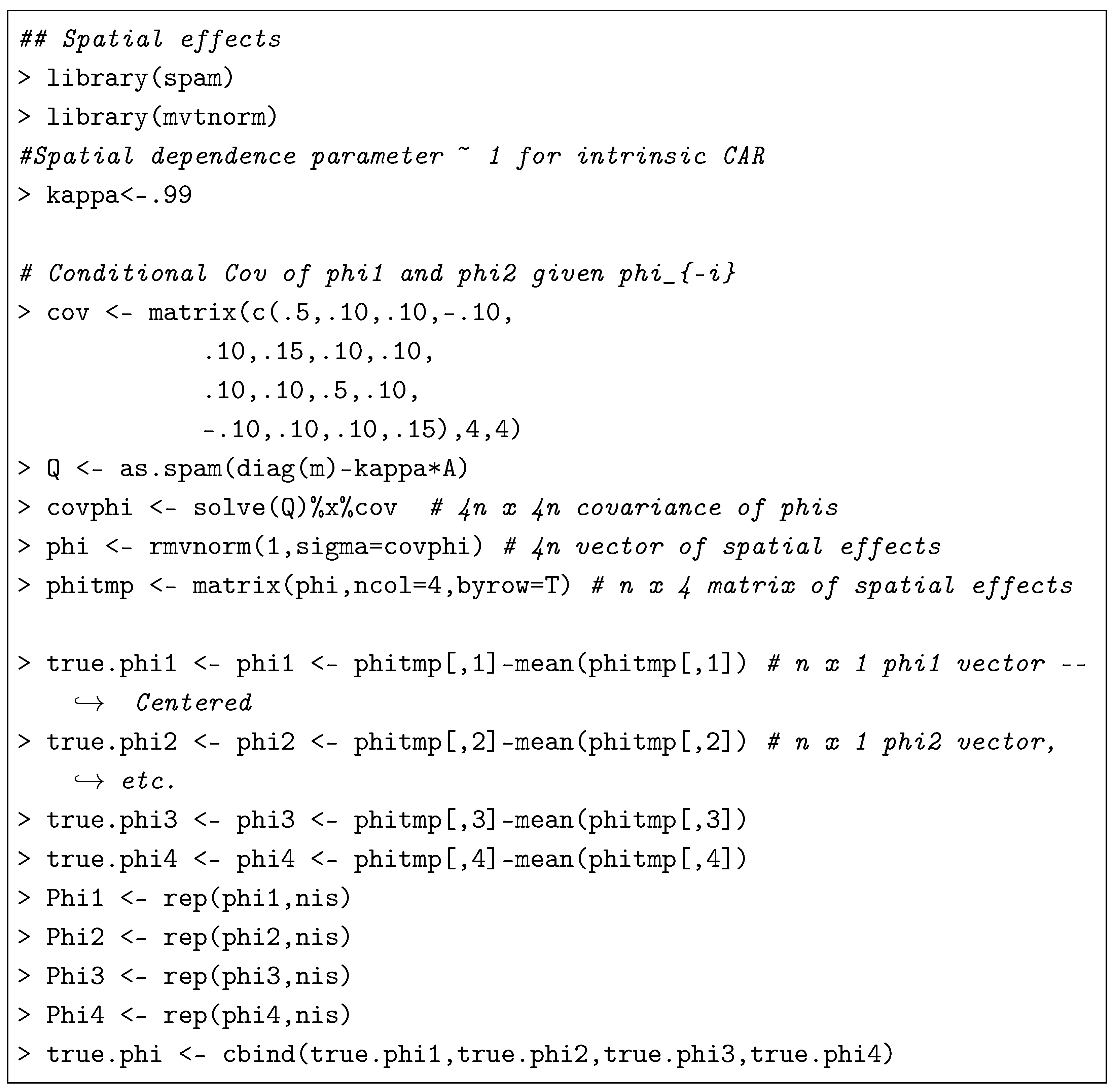
For the further data-generating process of our simulation, we set an intrinsic conditional autoregressive (ICAR) structure with a spatial dependence parameter ${\sigma }_b^2=1$ and a pre-specified conditional covariance matrix for ${\Phi }_1,{\Phi }_2,{\Phi }_3,{\Phi }_4$, defined in Section 2.3. This is set to check whether our model can properly adjust for the spatial dependence of the outcome.

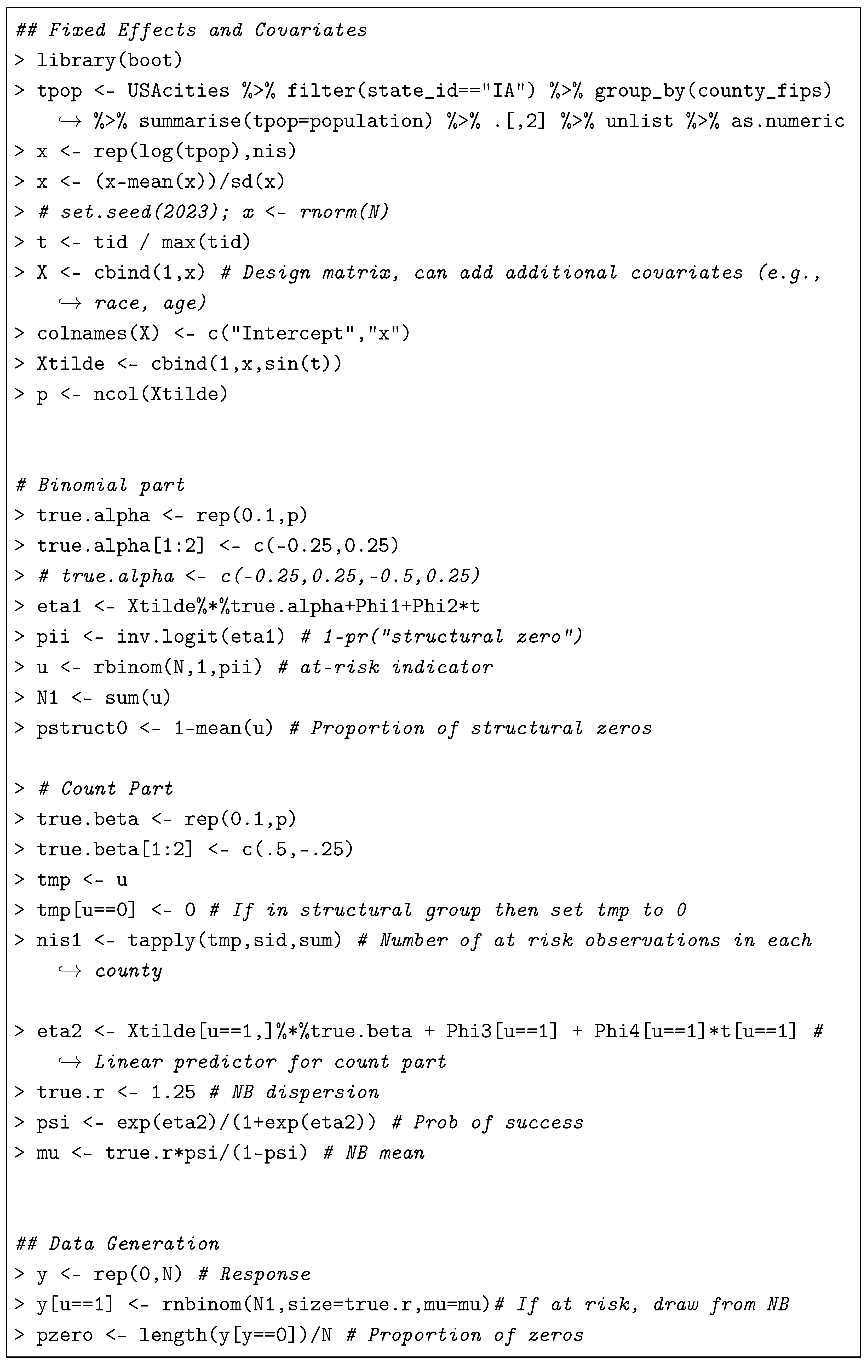
Following the data model Equation (1) and process model Equation (5), we specify the underlying at-risk-probability model as

$$logit\left(q_{ij}\right)=-0.25+0.25x_{ij}+0.10sin\left(t_{ij}\right)+{\Phi }_{1i}+{\Phi }_{2i}t,$$

for $i=1,\cdots ,99$ and $j=1,\cdots ,24$, and success-probability model as

$$logit\left(p_{ij}\right)=0.5-0.25x_{ij}+0.10sin\left(t_{ij}\right)+{\Phi }_{3i}+{\Phi }_{4i}t,$$

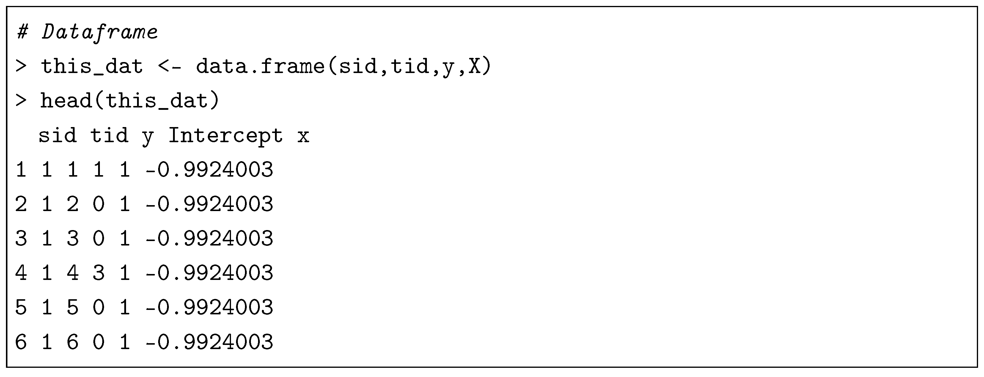
for $i=1,\cdots ,99$ and $j=1,\cdots ,24$, where ${\Phi }_{1i},\cdots ,{\Phi }_{4i}$ are mean-centered, random-generated quantities from the conditional covariance matrices ${\Phi }_1,{\Phi }_2,{\Phi }_3,{\Phi }_4$ based on Section 2.3. Finally, $y_{ij}$, i.e., an outcome count at the ith spatial unit and the jth time point, is assigned to either zero if $w_{ij}=0$, or a realized value from the Negative Binomial distribution. We use both a mean parameter of an inverse logit of $p_{ij}$ and a pre-specified dispersion parameter $r=1.25$, which consider both regression modeling in the risk probability and over-dispersion in outcome counts. We then combine all variables to create our data frame:

4.3. Descriptive Analysis

Table 2 shows a descriptive summary of data using the function tbl_summary from the gtsummary package. A continuous value is summarized by median and inter-quantile range (IQR), while a discrete value is summarized by counts and proportion.

Table 2. A descriptive summary table for the generated synthetic data.

Coefficients	N = 1584 1
sid	50 (25, 75)
tid	9 (5, 13)
y	0.00 (0.00, 1.00)
Intercept	1584 (100%)
x	−0.20 (−0.68, 0.38)

¹ Median (IQR); n (%).

Table 2. A descriptive summary table for the generated synthetic data.

Coefficients	N = 1584 1
sid	50 (25, 75)
tid	9 (5, 13)
y	0.00 (0.00, 1.00)
Intercept	1584 (100%)
x	−0.20 (−0.68, 0.38)

¹ Median (IQR); n (%).

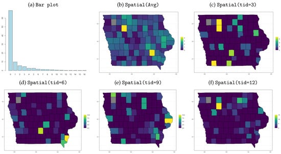
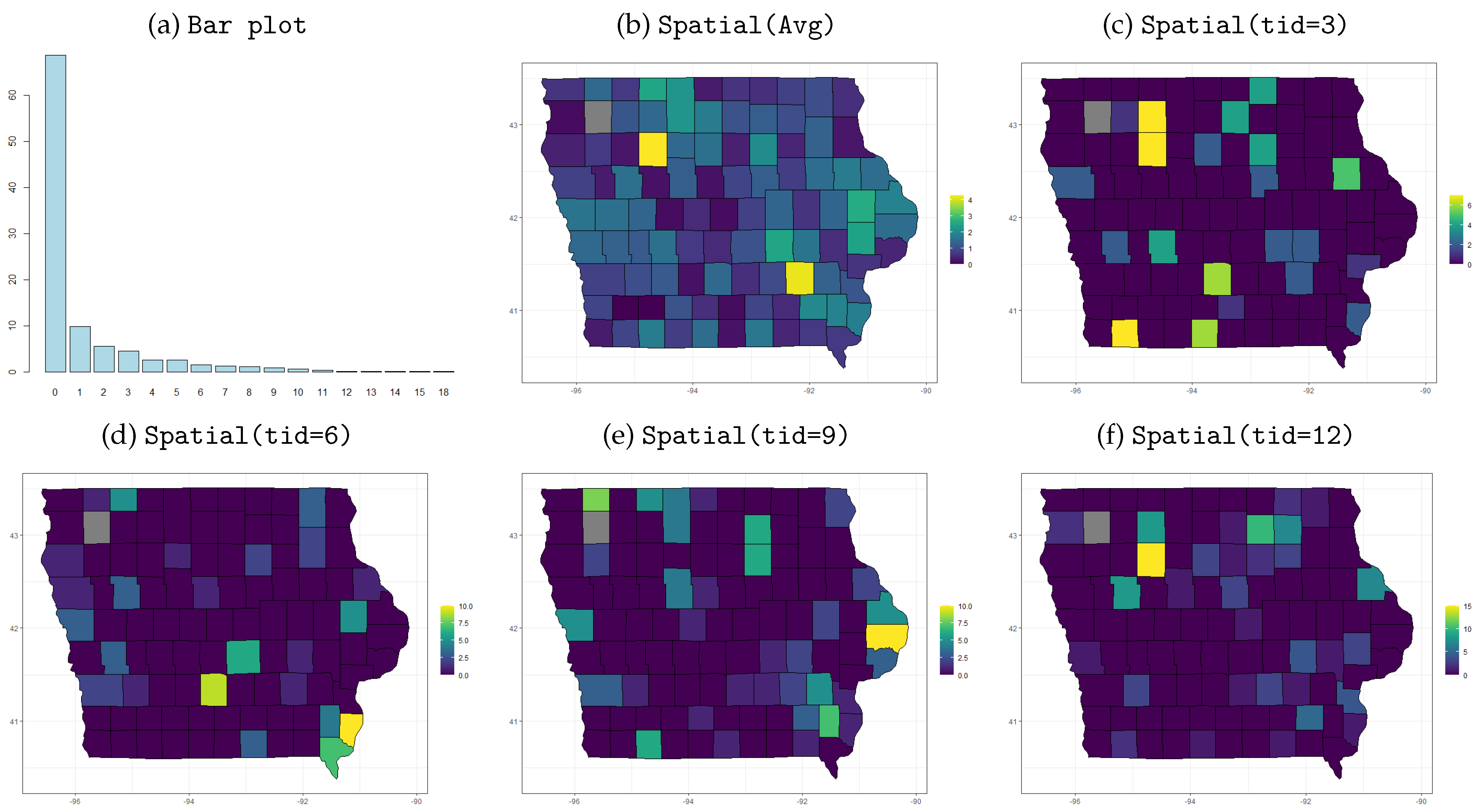
This script shows a histogram of all outcome counts (Figure 2a) for checking the proportions of zero counts. We observe a high proportion of zero counts (66.7%), supporting our zero-inflated distributional assumptions.

Figure 2. An example of descriptive summary of the outcome counts (y) for our simulation study. (a) Histogram of all outcome counts; (b) time-averaged spatial map visualization of outcome counts; (c–f) spatial map visualization of outcome counts at (c) $tid=3$, (d) $tid=6$, (e) $tid=9$, (f) $tid=12$.

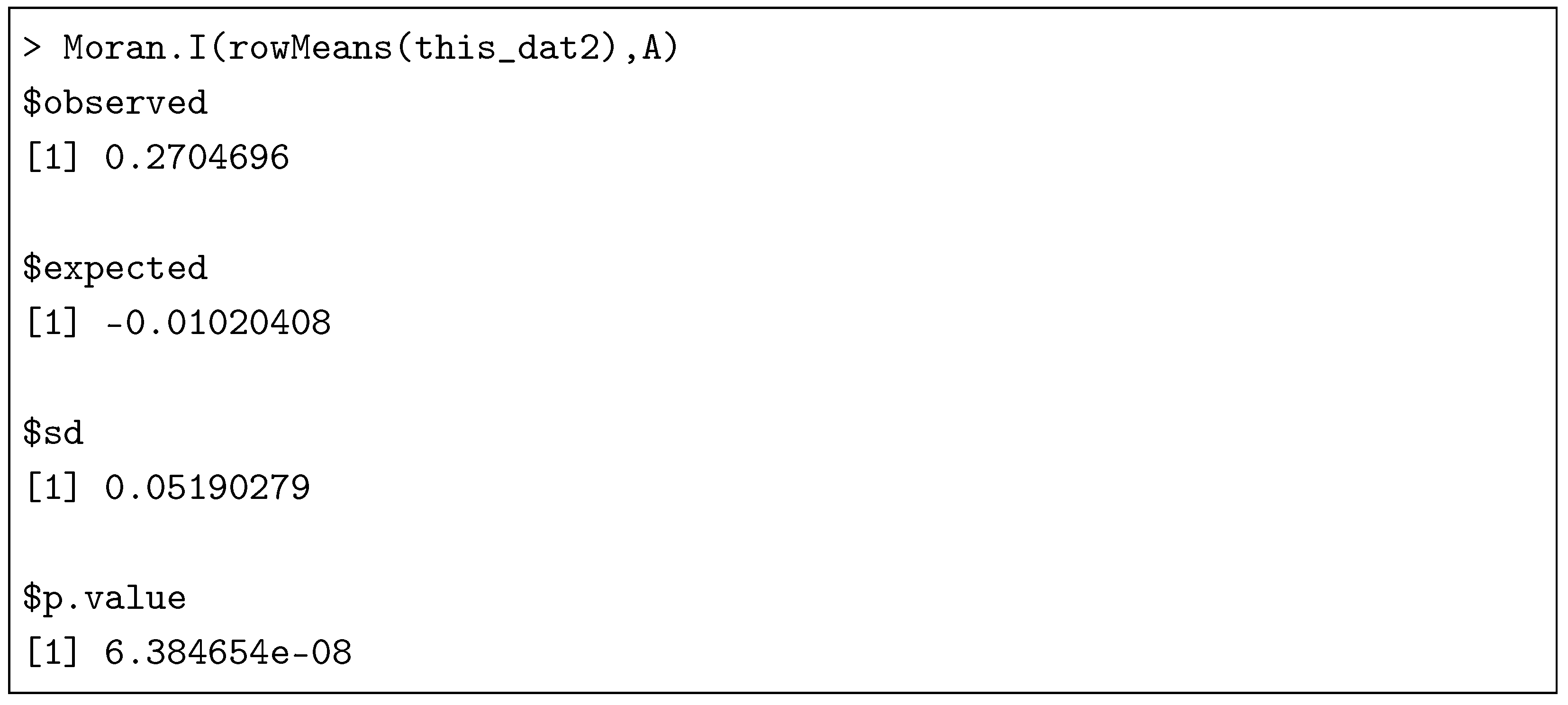
This script investigates the spatial aggregation of the disease counts over the counties. Moran.I is from the R-package ape. The estimated Moran’s I statistics for the time-averaged disease counts are statistically significant because its p-value $=4.46\times {10}^{-16}$ is lower than the 5% nominal Type I error. Also, Moran’s I statistics calculated for each time index are all less than 5% nominal Type I error. These results support our spatial random effect modeling of the target outcome since we observe a spatial clustering tendency of the outcome, albeit the covariates are independent of spatial locations.  

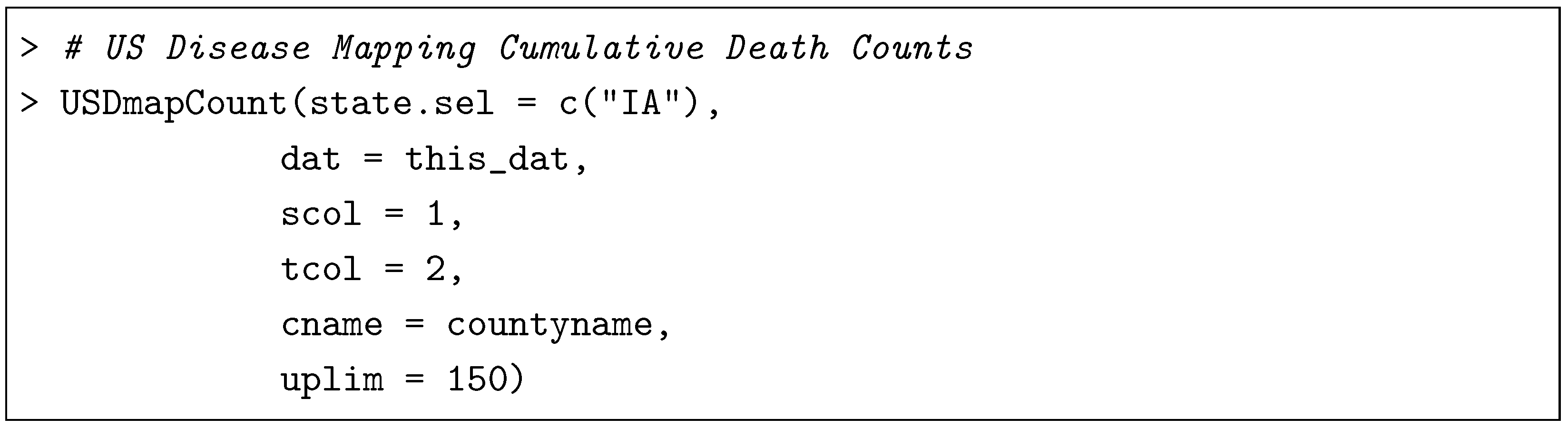
USDmapCount in our package visualizes a map of disease characteristics in the United States. For example, the above script recognizes the Iowa state as a study domain, this_dat as input data, including spatial index in the column scol and time index in the column tcol. We can manually set the name of counties using the cname argument and scale of the legend color using uplim. If we further specify tsel, we can select counts in a specific time point. Otherwise, counts are averaged over time. Figure 2b–f implies the spatio-temporal relation of the disease counts. Compared to the time-average case from the above statement (Figure 2b), all the time-specific cases (Figure 2c–f) show different patterns, which may indicate spatio-temporal dependence of the disease counts. This descriptive analysis implies that naive Negative Binomial modeling without incorporating spatio-temporal dependence may produce biased and/or inefficient estimates.

4.4. Bayesian Spatio-Temporal Modeling

We implement the Bayesian regression modeling of the disease counts that allows not only over-dispersion but also a high proportion of zero counts and a spatio-temporal nature. Our package provides several Bayesian Negative Binomial models such as the BNB function for a standard model; the BZINB function for considering a zero-inflated model component (see Section 2.1); the BSTNB function for the considering the spatio-temporal random effect model component (see Section 2.2); and the BSTZINB function for the Bayesian spatio-temporal zero-inflated model (see Section 2.3). For instance, we apply the BSTZINB function to this example as follows:

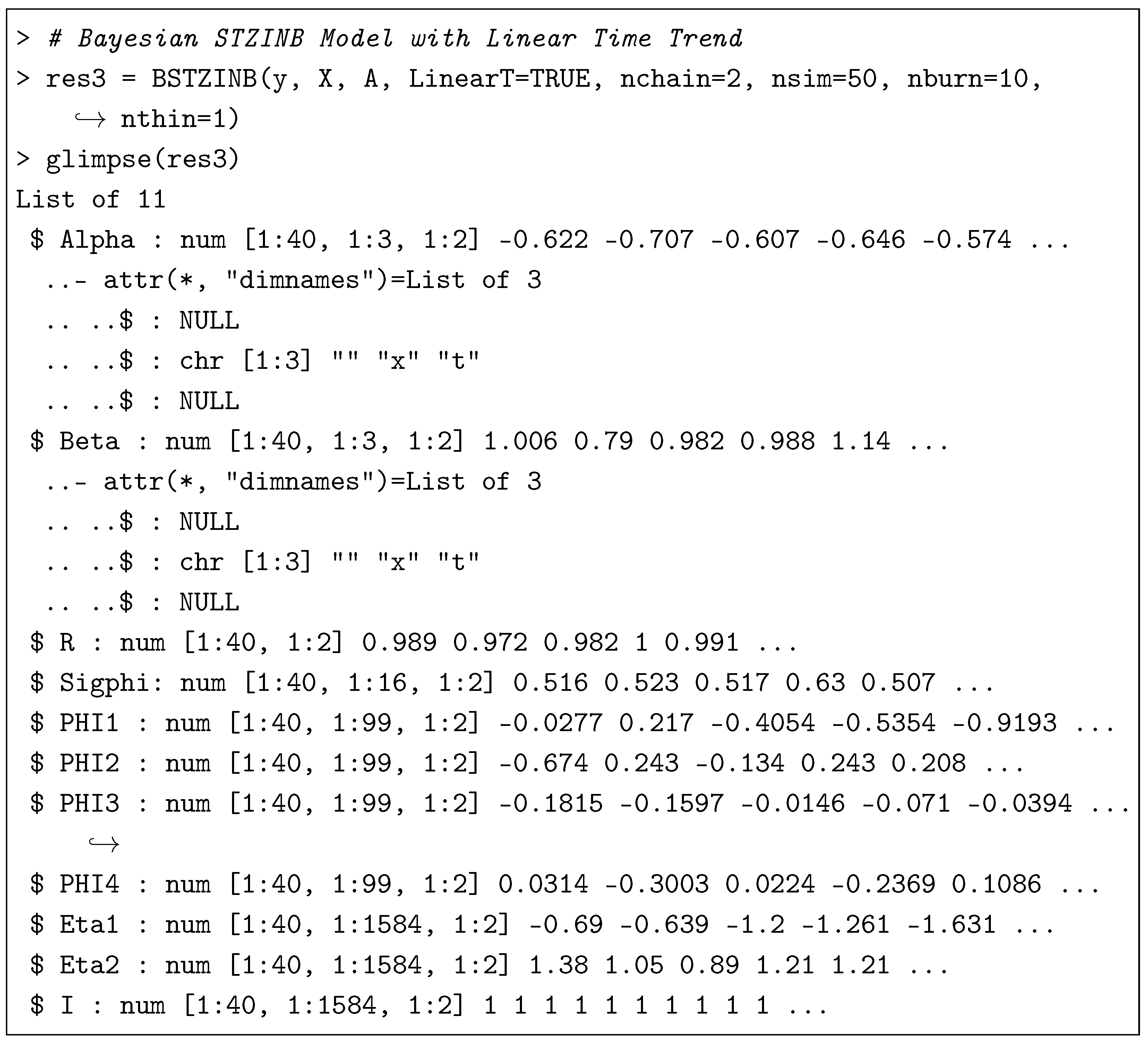
We have added an example for LinearT=FALSE in the online vignette that is available with the R package from CRAN: https://cran.r-project.org/web/packages/BSTZINB/vignettes/BSTZINB_vignette.html (accessed on 13 July 2026), look into the example res4 <- BSTZINB(y, X, A, LinearT=FALSE, nchain=2, niter=50, nburn=10).

We illustrate the major interpretations and visualizations in the following subsections based on the above run model.

4.4.1. Main Results

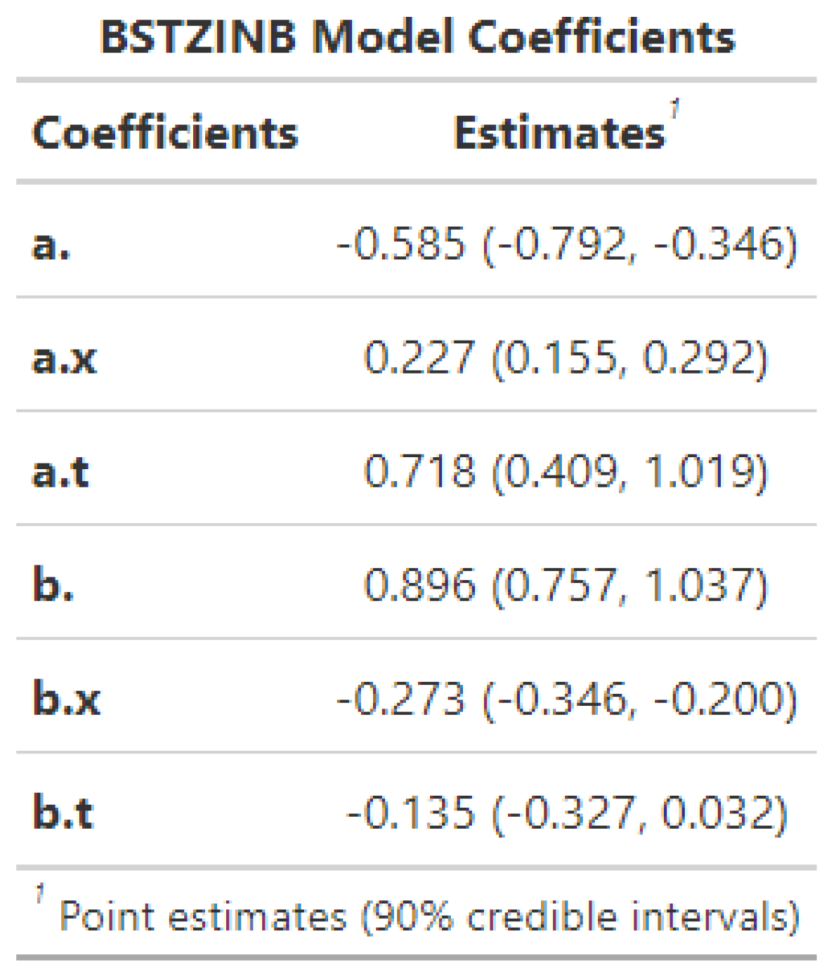
ResultTableSummary transforms the BSTZINB object into a brief summary table, as shown in Figure 3. The first column of the table shows a list of regression coefficients, where combinations of an alphabet and a specified column name are used. The alphabet is either ‘a’ or ‘b,’ where ‘a’ refers to the structural zero model coefficients, and ‘b’ refers to the exposure model coefficients. If a column name is not specified, no letters will appear right after the period, but otherwise, the specified name will followed by the period.

For example, “b.x” means the coefficient of the covariate named “x” in the exposure model components. “a.” means the coefficient without any specified name in the structure-zero model components. On the other hand, the second column of the table shows relevant statistics. The first row shows the total number of observations, and the other rows provide point estimates and a 90% credible interval in parentheses.

Figure 3. ResultTableSummary produces a brief summary table of the BSTZINB object. Here ‘a’ refers to the structural zero model coefficients and ‘b’ refers to the exposure model coefficients. ‘a.’ refers to the intercept coefficient for the structural zero model, while ‘b.x’ refers to the coefficient related to covariate x in the exposure model.

Figure 3. ResultTableSummary produces a brief summary table of the BSTZINB object. Here ‘a’ refers to the structural zero model coefficients and ‘b’ refers to the exposure model coefficients. ‘a.’ refers to the intercept coefficient for the structural zero model, while ‘b.x’ refers to the coefficient related to covariate x in the exposure model.

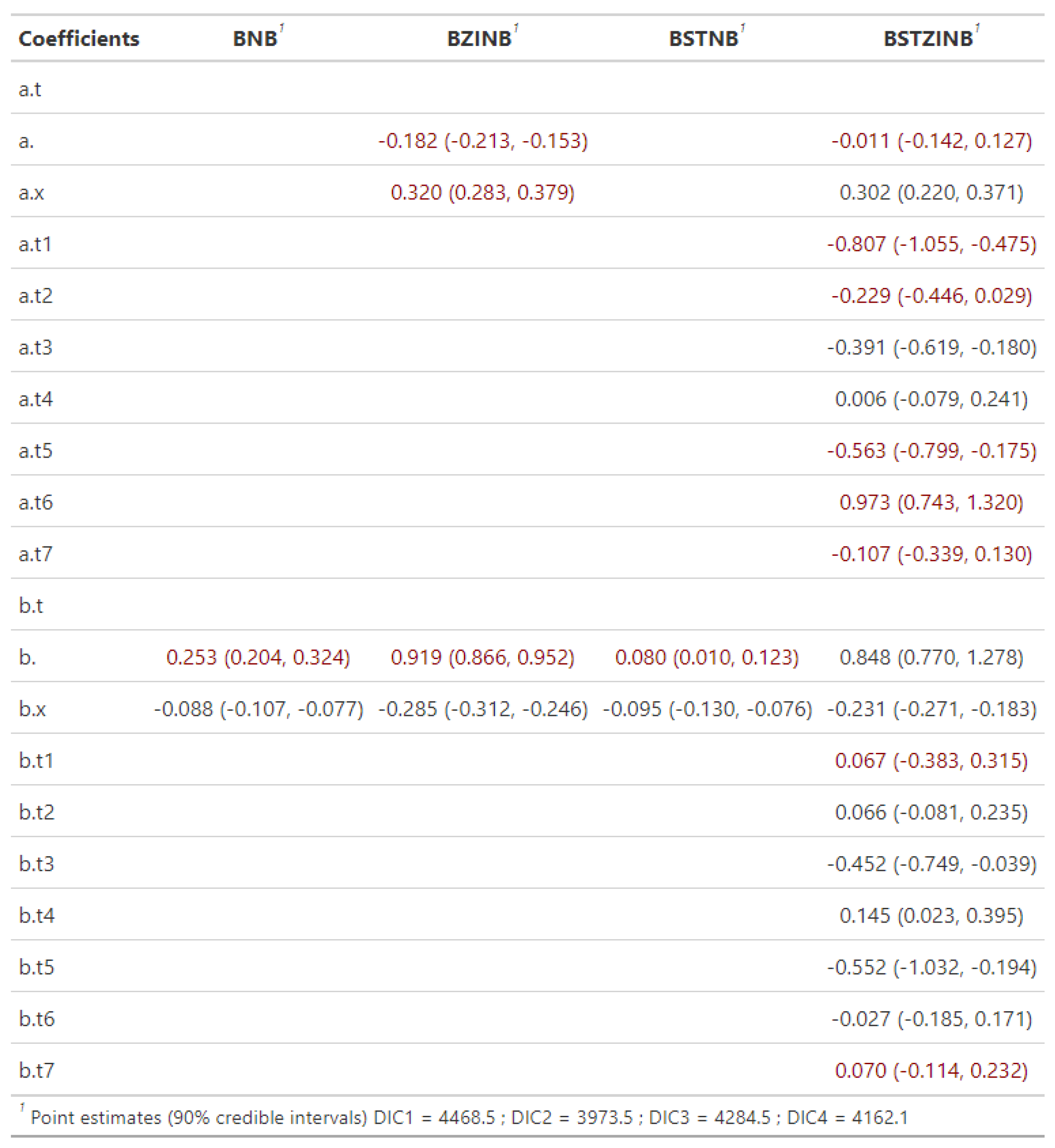
ResultTableSummary2 performs all Bayesian spatio-temporal model procedures available in the package, including BNB, BZINB, BSTNB, and BSTZINB, providing a full summary table, as shown in Figure A1. Note that the model coefficients of the time spline basis vectors are followed by those of the input covariates. For example, assuming the BSTZINB-NLT model (Section 2.3), $(a.,a.x,a.t1,a.t2,a.t3,a.t4,a.t5,a.t6,a.t7)$ corresponds to $({\beta }_{10},{\beta }_{11},{\beta }_{12},{\beta }_{13},{\beta }_{14},{\beta }_{15},{\beta }_{16},{\beta }_{17})$ in Equation (5), where $D_1=1$, and $M=6$. A red-colored text represents a failure to achieve MCMC convergence using Geweke statistic [25]. Also, a footnote provides the Deviance Information Criterion (DIC) as a model selection tool. The fourth model BSTZINB has the lowest DIC value with the given example data.

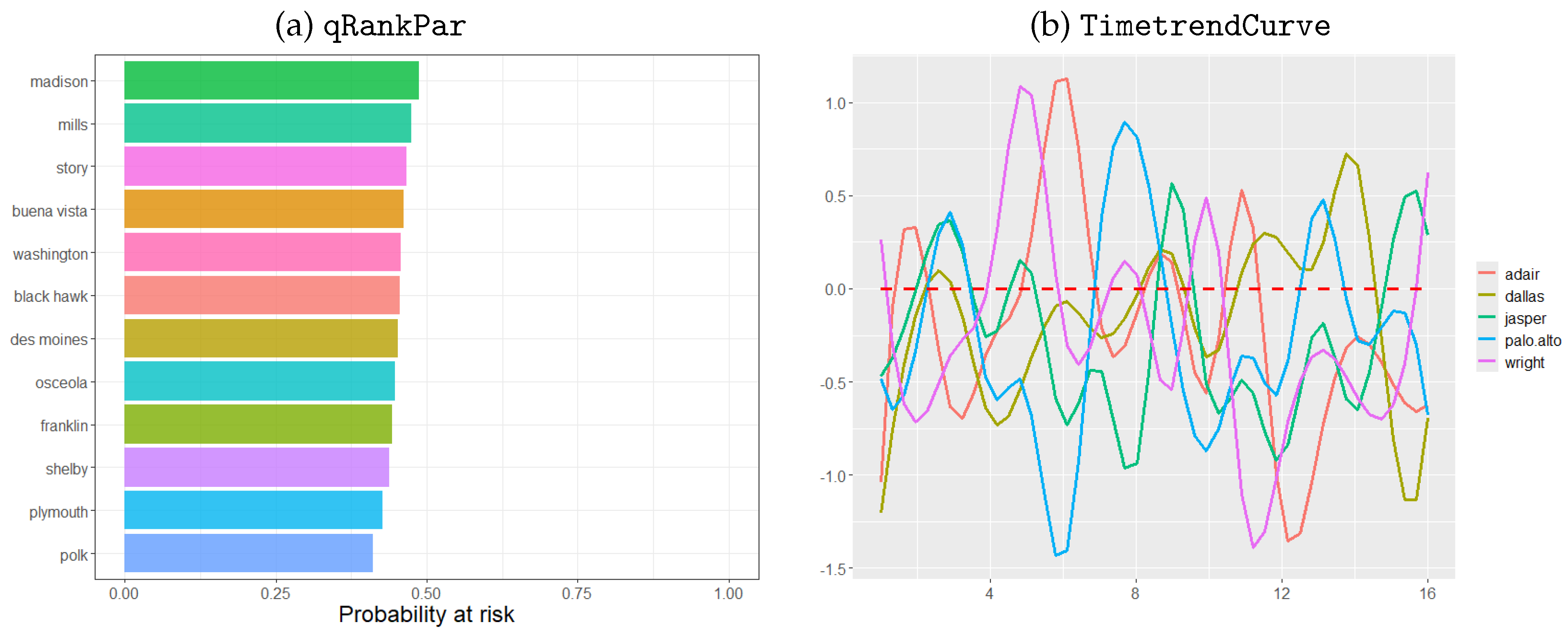
qRankPar produces a bar plot of time-averaged estimated disease probabilities at risk, taking into account the quantiles and the descending order of the rankings among spatial units. For example, the argument $\mathtt{v}\mathtt{n}=12$ decides the number of selected counties. That is, we choose the counties out of a given map considering $\mathtt{v}\mathtt{n}=12$ quantiles of estimated disease probabilities from the BSTZINB object.

qRankParTop produces a bar plot for time-averaged estimated disease probabilities at risk for selected counties in descending order (Figure 4a). The options cex.title, cex.lab and cex.legend control the text size for the title, labels, and legend, respectively.

Figure 4. An illustrative example of eta-related results. (a) The left panel shows a result from the function qRankPar, producing a bar plot for time-averaged estimated disease probability at risk considering the rankings’ quantiles and descending order. (b) The right panel shows a result from the function TimetrendCurve, producing the estimated nonlinear mixed time effects in the Negative Binomial model component.

TimetrendCurve produces the estimated nonlinear mixed time effects in the Negative Binomial model component (See Figure 3 in [1]).

The argument smooth.mode=T produces the cubic-spline interpolated nonlinear mixed time effects (Figure 4b). The options cex.title, cex.lab and cex.legend work as described previously.

4.4.2. Map Visualization

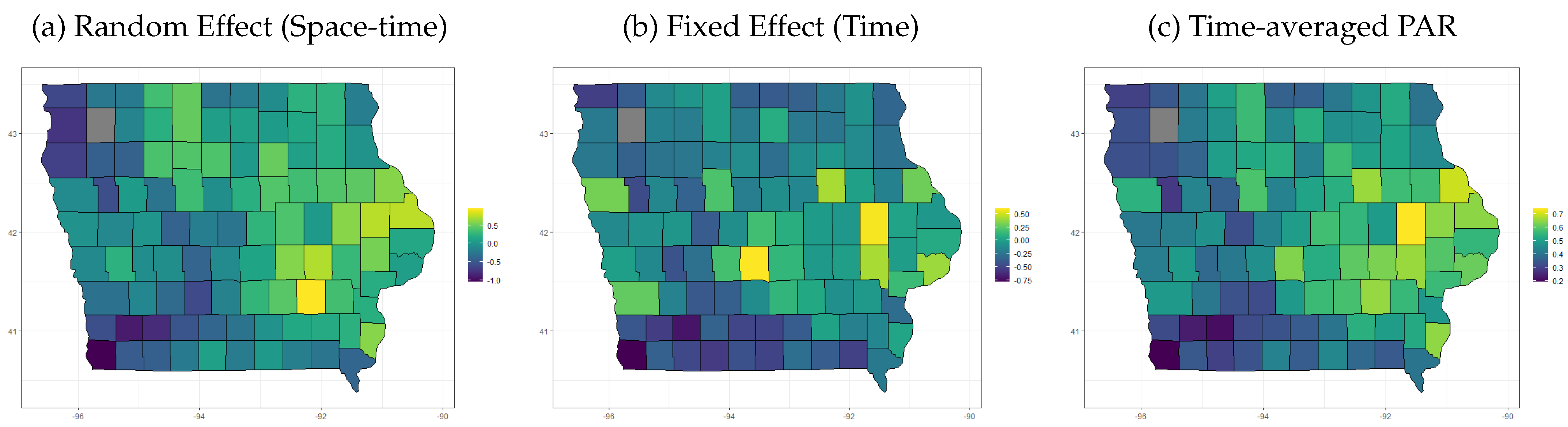
We describe several map visualizations based on the results above. The function USDmapCount visualizes the time-averaged disease counts over the counties in the United States. The x-axis represents longitude, the y-axis represents latitude, and the color indicates the level of disease counts. Missing values are shown in gray.

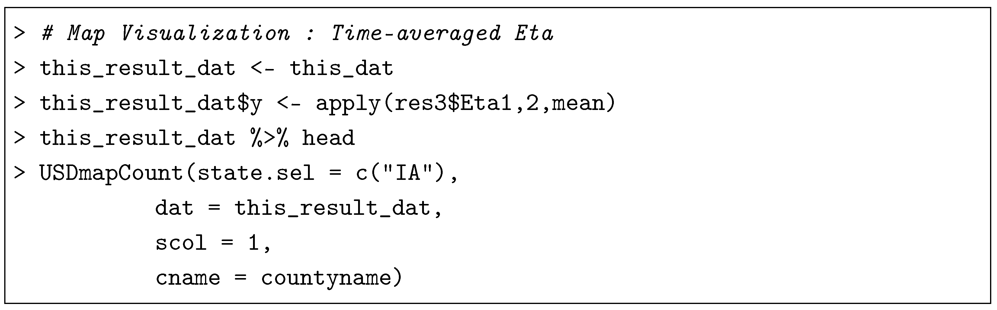
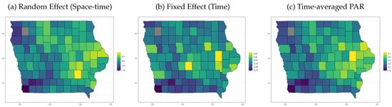
If a user sets a dat argument as ${\eta }_1$ from the BSTZINB output, then the outcome will provide a spatial visualization of the logit of the estimated probability at risk on average over time. Likewise, we can provide a map of the following characteristics from the model fitting (see Figure 5).

Figure 5. Map visualizations of various estimates regarding spatio-temporal aspects of health outcome. (a) The level of spatio-temporal random effect; (b) the level of temporal fixed effect; (c) time-averaged disease probability at risk (PAR).

4.4.3. MCMC Convergence and Diagnostics

The BNB, BZINB, BSTNB, and BSTZINB functions can provide console messages about work progress while running. This includes chains, iterations, and diagnostics in MCMC samplings. For example, we can see the following line on the R-console:

This means that the first chain out of the two chains (specified from the argument nchain) is currently processing, 85% of the samples are completed to be generated, and those samples passed the Geweke convergence test. In particular, TRUE means pass, FALSE means fail, and NA means not applicable since the MCMC samplings are still in the burn-in period.

Our package also provides the Geweke convergence test after completing the Bayesian model fitting. For example, we can check MCMC convergence for each of the BSTZINB model parameters as follows:

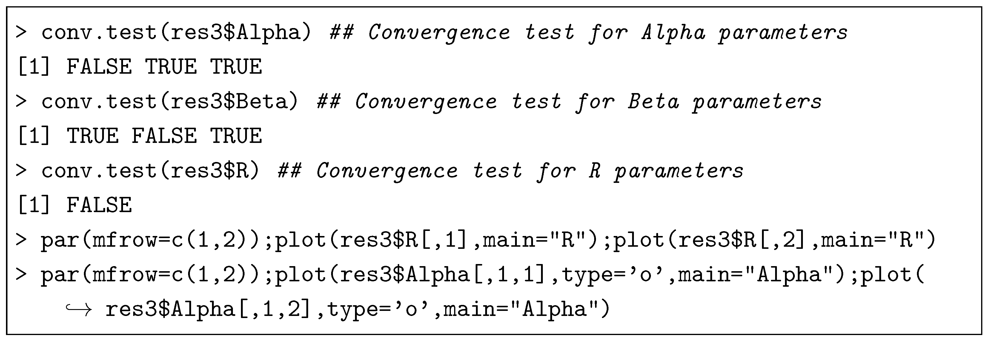
Recall that res3 is made from a Bayesian spatio-temporal zero-inflated Negative Binomial model with a linear time trend. This model has three alpha coefficients for the structural zero model component, three beta coefficients for the Negative Binomial model component, and one dispersion parameter. Our built-in function conv.test shows test results for each parameter sample. TRUE means statistical evidence on the convergence of the samples based on the Geweke test. In addition, you can generate trace plots to check stationarity and a degree of mixingness and visualize convergence behaviors of the MCMC samples [26].

compute_NB_DIC and compute_ZINB_DIC compute the Deviance Information Criterion specifically designed for the BSTNB and BSTZINB model outputs, respectively [27,28].

5. Discussion and Conclusions

The BSTZINB R-package tackles spatial and temporal analysis of health outcomes in epidemiology. It offers a three-phase framework: Phase 1 checks if your data suits the model by examining zero proportions and spatial/temporal dependencies. Phase 2 tackles data with zero inflation or non-standard dispersion using Bayesian inference. Finally, Phase 3 generates reports including health effect estimates, maps, and results from the model.

The BSTZINB R-package stands out for its focus on usability, making it accessible to researchers in epidemiology and beyond, even those without a deep dive into statistics. This practitioner-friendly design prioritizes ease of use, allowing researchers from any academic or industrial field to leverage powerful spatio-temporal methods without getting bogged down in complex mathematical details. The package comes equipped with clear, well-designed case studies that serve as practical guides for users to follow, ensuring they can confidently apply these methods to their own research questions.

The BSTZINB R-package goes beyond user-friendliness. It streamlines the workflow by unifying existing R tools under a coherent Bayesian framework, boosting efficiency and consistency in spatio-temporal modeling and inference. This powerhouse caters to the complexities of epidemiological data by incorporating zero-inflated count data and flexible random effects that can vary across space and time. Moreover, the freely available, open-source nature of the package makes it accessible to a broad range of researchers, fostering collaboration within the field. Looking ahead, addressing potential limitations like computational hurdles for massive datasets and the need for further development in advanced tools like R-Stan [29] will solidify BSTZINB’s position as a premier tool for spatio-temporal analysis in epidemiology. It is important to note here that any Stan-based development would require careful reformulation, such as marginalizing over the discrete at-risk indicators where possible, using continuous relaxations, or embedding Stan within a larger MCMC scheme that alternates between updates of discrete latent indicators and continuous model parameters.

Despite its flexibility, BSTZINB inherits the computational limitations common to MCMC-based Bayesian spatio-temporal models. The current implementation is best suited for small- to moderate-scale areal datasets, where reliable posterior inference can be obtained within reasonable computation times. As the number of spatial units, temporal observations, and model parameters increases, computational cost grows accordingly. Future enhancements will focus on improving scalability, expanding prior flexibility, and incorporating more computationally efficient Bayesian inference strategies.

It is important to emphasize that the primary objective of the BSTZINB package is to provide Bayesian inference tools for spatio-temporal zero-inflated count outcomes commonly encountered in epidemiology, public health, and environmental studies. Consequently, survival-analysis frameworks based on lifetime distributions such as the exponential or Weibull distributions, as well as competing-risk models, fall outside the intended scope of the current package and correspond to fundamentally different classes of outcomes and inferential objectives. Rather than focusing on time-to-event data, BSTZINB is specifically designed for count data exhibiting excess zeros, over-dispersion, and spatio-temporal dependence. Nevertheless, the underlying Bayesian framework is sufficiently flexible that future extensions could incorporate broader classes of outcomes, including survival, recurrent-event, and competing-risk data, thereby expanding the applicability of the package to a wider range of biomedical and epidemiological research settings.

In closing, the BSTZINB R-package is a significant advancement in analyzing data that changes over space and time in epidemiology. Even researchers new to statistics can easily use it. BSTZINB combines modern statistical methods with helpful visualization tools. This makes it a powerful and flexible option for analyzing such data in many fields, including epidemiology, biostatistics, and environmental science. While BSTZINB excels at making complex methods easier to use and understand, there’s room for improvement. Future development can address handling very large datasets and include even more advanced models. These improvements will solidify BSTZINB’s position as a leading tool for spatio-temporal analysis in epidemiology and beyond.

Appendix A.1. Bayesian Inference

We illustrate prior and hyper-parameter specifications and Markov Chain Monte Carlo (MCMC) settings under the STZINB model framework. For the latent at-risk indicators $w_{ij}$, probability was given as $exp\left({\theta }_{1ij}\right)/[1+exp\left({\theta }_{1ij}\right)]$, where ${\theta }_{1ij}$ is defined as either Equation (5) or (8). Prior distributions for ${\mathit{\beta }}_1$ and ${\mathit{\beta }}_2$ were assumed to be $N_p\left({\beta }_0=\mathbf{0},{\Sigma }_0=100{\mathcal{I}}_p\right)$, respectively, where ${\mathcal{I}}_p$ is a $p\times p$ identity matrix. For r in Negative Binomial component, a uniform prior was considered. To construct time-basis functions $T_m,m=1,\cdots ,M$, we standardized time points $t_{ij}$ to be within the range of 0 to 1, i.e., $t_{ij}={\displaystyle \frac{j}{J}}$, where $J=23$ is the number of weeks during the study period, and $j=1,\cdots ,J=23$ is a week indicator. We set three internal knot points, 0.25, 0.50, and 0.75, considering 0 and 1 as boundaries, so that $M=7$ throughout our analysis. DIC is calculated as described in [30] for model comparison.

For each model, we ran three MCMC chains with 11,000 iterations and 1000 burn-in. For each model, the convergence of each model was determined by conventional MCMC diagnostics such as trace plots and Geweke z-statistics.

Appendix A.2. Model Fitting Principles

We adopt a posterior sampling algorithm from Neelon et al. (2019) [17] and Chakraborty et al. (2022) [1], which can be extended straightforwardly to other simpler models. As outlined in Chakraborty et al. (2022) [1], we update several key parameters including at-risk indicators $\mathit{w}$, coefficients ${\mathit{\beta }}_1$ for the binary model component, coefficients ${\mathit{\beta }}_2$ for the count model component, a dispersion parameter r for the Negative Binomial distribution, and spatial random effects $\mathit{\varphi }$ with $\Gamma$. The following steps describe the MCMC algorithm used to update these parameters.

• Update at-risk indicators $\mathit{w}$
  We draw $w_{ij}$ from a Bernoulli distribution with probability ${\eta }_{ij}$ defined as:

  $${\eta }_{ij}={\displaystyle \frac{q_{ij}^r(1-p_{ij})}{q_{ij}^r(1-p_{ij})+p_{ij}}}$$

  (A1)

  where $q_{ij}$ and $p_{ij}$ are functions illustrated in Section 2.3, given current parameter values. To avoid numerical issues, $q_{ij}$ and $p_{ij}$ are adjusted to be within $(0.001,0.999)$ in practice.
• Update $\mathit{\beta }=({\mathit{\beta }}_1,{\mathit{\beta }}_2)$
  We draw a latent variable ${\xi }_{1ij}$ from a Pólya-Gamma distribution $PG(1,{\theta }_{1ij})$, and update ${\mathit{\beta }}_1$ using its full conditional distribution based on observed data and prior distributions. Updating ${\mathit{\beta }}_2$ follows a similar process using the Pólya-Gamma distribution $PG(y_{ij}+r,{\theta }_{2ij})$.
• Update r
  We employ a random-walk Metropolis-Hastings step for updating r, as detailed in [17], with a uniform prior for computational efficiency.
• Update $\mathit{\varphi }$, $\Gamma$
  We update $\mathit{\varphi }$, which consists of random effects vectors, from their normal full conditional distributions. The update involves applying sum-to-zero constraints where necessary. The spatial structure $\Gamma$ is updated using an inverse-Wishart full conditional distribution (described in detail [1]).

Appendix A.3. Additional Tables and Figures

Figure A1. ResultTableSummary2 produces a full summary table of the BSTZINB object. For the column “Coefficients”, “a.*” stands for structural zero model coefficients, and “b.*” stands for exposure model coefficients. “*.t” implies coefficients for time variables, and “*.x” implies coefficients for covariates x’s, and “*.” means an intercept. From “*.t1” to “*.t7” represents the corresponding spline basis functions applied in the BSTZINB models (when LinearT = FALSE). Each cell shows the point estimate and the 90% credible interval within the parenthesis. Red colors represent the poor convergence of the estimates. Other terminologies are defined as follows: BSTP—Bayesian Spatio-Temporal Poisson; BSTNB—Bayesian Spatio-Temporal Negative Binomial; BSTZINB(LT)—Bayesian Spatio-Temporal Zero Inflated Negative Binomial with linear temporal fixed effect on the structural zero model component; BSTZINB(NLT)—Bayesian Spatio-Temporal Zero Inflated Negative Binomial with a non-linear temporal fixed effect on the structural zero model component.

Figure A1. ResultTableSummary2 produces a full summary table of the BSTZINB object. For the column “Coefficients”, “a.*” stands for structural zero model coefficients, and “b.*” stands for exposure model coefficients. “*.t” implies coefficients for time variables, and “*.x” implies coefficients for covariates x’s, and “*.” means an intercept. From “*.t1” to “*.t7” represents the corresponding spline basis functions applied in the BSTZINB models (when LinearT = FALSE). Each cell shows the point estimate and the 90% credible interval within the parenthesis. Red colors represent the poor convergence of the estimates. Other terminologies are defined as follows: BSTP—Bayesian Spatio-Temporal Poisson; BSTNB—Bayesian Spatio-Temporal Negative Binomial; BSTZINB(LT)—Bayesian Spatio-Temporal Zero Inflated Negative Binomial with linear temporal fixed effect on the structural zero model component; BSTZINB(NLT)—Bayesian Spatio-Temporal Zero Inflated Negative Binomial with a non-linear temporal fixed effect on the structural zero model component.

Appendix B.1. Data

A data frame with 4 variables: Countyname—2010 state and county name; fips.County—2010 state and county FIPS codes; neighborname—2010 state and county name of each neighboring county or county equivalent; fipsneighbor—2010 state and county FIPS codes of each neighboring county or county equivalent (See this link from the census.gov: https://www.census.gov/geographies/reference-files/2010/geo/county-adjacency.html#:~:text=The%202010%20county%20adjacency%20file%20is%20a%20national%2C%20tab%20delimited,the%20end%20of%20the%20list, accessed on 13 July 2026).

A data frame with 17 variables: city—The name of the city/town; city_ascii—“city” as an ASCII string; state_id—the state or territory’s USPS postal abbreviation; state_name—the name of the state or territory that contains the city/town; county_fips—the 5-digit FIPS code for the primary county. The first two digits correspond to the state’s FIPS code; county_name—the name of the primary county (or equivalent) that contains the city/town; lat—the latitude of the city/town; lng—the longitude of the city/town; population—an estimate of the city’s urban population; density—the estimated population per square kilometer; source—for some cities, our data is generated from a polygon representing the city, for others we simply have a point; military—TRUE if this place is a military establishment such as a fort or base; incorporated—TRUE if the place is a city/town. FALSE if the place is just a commonly known name for a populated area; timezone—the city’s time zone in the tz database format (e.g., America/Los_Angeles); ranking—an integer from 1-5 that captures the importance of a city (1 is most important, 5 least important); zips—a string containing all five-digit zip codes in the city/town, delimited by a space. Learn more; id—a 10-digit unique id generated by SimpleMaps. It is consistent across releases and databases (e.g., World Cities Database) (see this link for US cities: https://simplemaps.com/data/us-cities, accessed on 13 July 2026).

Appendix B.2. Main Functions

BNB, BZINB, BSTNB, and BSTZINB are considered as main functions in our package. Here, we are only illustrating the BSTZINB function since the other functions are just a few variants.

• y: A response variable in a vector form of size n. Our model assumes y is arranged in ascending order of spatial unit and temporal unit. For example, if we assume s spatial units and t temporal unit, then we consider y of size $n=st$ as arranged in the following order: $(1,1),(1,2),\cdots ,(1,t),(2,1),(2,2),\dots ,(s,t)$
• X: A set of covariates in a matrix form. It has n rows indicating spatio-temporal unit, and p columns indicating each covariate.
• A: Adjacency matrix of which $(i,i^{\prime })$ element is either 1 if spatial unit i and $i^{\prime }$ are neighbors, or 0 otherwise.
• LinearT: A logical indicator. The default option is TRUE. TRUE means that we assume a linear time trend structure. FALSE means that we assume a non-linear time trend structure represented by B-spline functions (See the reference).
• nchain: The number of chains in MCMC settings.
• niter: The number of iterations in MCMC settings.
• nburn: The number of burn-in samples in MCMC settings.
• nthin: The number of thinning samples in MCMC settings.

The output of the BSTZINB function consists of the following:

• Alpha: MCMC sampled coefficients in the binary (structure zero) model component.
• Beta: MCMC sampled coefficients in the count (Negative Binomial) model component.
• R: MCMC sampled dispersion parameters using the random-walk Metropolis–Hastings approach.
• R2: MCMC sampled dispersion parameter using the two-stage Gibbs approach.
• Sigphi: MCMC Sampled values of the $4\times 4$ conditional covariance matrix $\Gamma$.
• PHI1: MCMC Sampled values of random intercepts for the binary (structure zero) model component.
• PHI2: MCMC Sampled values of random slopes for the binary (structure zero) model component.
• PHI3: MCMC Sampled values of random intercepts for the count (Negative Binomial) model component.
• PHI4: MCMC Sampled values of random slopes for the count (Negative Binomial) model component.
• ETA1: MCMC Sampled values of $logit\left(q_{ij}\right)$ for the binary (structure zero) model component.
• ETA2: MCMC Sampled values of $logit\left(p_{ij}\right)$ for the count (Negative Binomial) model component.

Appendix B.3. Auxiliary Functions

The following are descriptions for a list of functions other than the main functions provided in Table 1.

• state.sel: A name set of states in the United States
• dat: A dataset with spatial and/or temporal unit variables.
• scol: An index or indexes of spatial unit variables in dat.
• tcol: An index of temporal unit variables in dat.
• tsel: A value of temporal units in dat. tsel=NULL is a default option, which shows a time-averaged output. You may specify a specific time value to show a time-specific output.
• cname: A name or a set of names of US counties.
• uplim: An upper limit value of outcome variables to visualize. uplim=NULL is a default option, which considers a maximum value of outcome variables to visualize.

• county.adjacency: A dataset of US counties including county names and their neighbors. county.adjacency (See Appendix B.1) is an exemplary dataset provided in our package.
• Countyvec: A set of names of US counties on your data analysis. All the counties should belong to the US states specified in the Statevec argument.
• Statevec: A set of names of US states on your data analysis.

qRankPar and qRankParTop have similar arguments to use, so we will only illustrate qRankParTop as their representative one.

• state.set: A name set of states in the United States.
• cname: A name or a set of names of US counties.
• bstfit: One of the BSTNB, or BSTZINB objects in our package.
• vn: The number of selected counties to visualize.
• cex.title: Font size for the title of the graph (in points).
• cex.lab: Font size for the labels on the axes (in points).
• cex.legend: Font size for the legend text (in points).

• bstfit: One of the BSTNB, or BSTZINB objects in our package.
• cname: A name or a set of names of US counties.
• vn: The number of selected counties to visualize.
• smooth.mode: TRUE if you apply smoothing spline approach to visualize ${\eta }_1$ (default); FALSE if you visualize a raw line of ${\eta }_1$
• cex.title: Font size for the title of the graph (in points).
• cex.lab: Font size for the labels on the axes (in points).
• cex.legend: Font size for the legend text (in points).

• bstfit: One of the BNB, BZINB, BSTNB, or BSTZINB objects in our package.

• y: A response variable in a vector form of size n. Our model assumes y is arranged in ascending order of spatial unit and temporal unit. For example, if we assume s spatial units and t temporal unit, then we consider y of size $n=st$ as arranged in the following order: $(1,1),(1,2),\cdots ,(1,t),(2,1),(2,2),\cdots ,(s,t)$
• X: A set of covariates in a matrix form. It has n rows indicating spatio-temporal unit, and p columns indicating each covariate.
• A: Adjacency matrix of which $(i,i^{\prime })$ element is either 1 if spatial unit i and $i^{\prime }$ are neighbors, or 0 otherwise.
• LinearT: A logical indicator. The default option is TRUE. TRUE means that we assume a linear time trend structure. FALSE means that we assume a non-linear time trend structure represented by B-spline functions (see the reference).
• nchain: The number of chains in MCMC settings.
• niter: The number of iterations per chain in MCMC settings.
• nburn: The number of burn-in samples per chain in MCMC settings.
• nthin: The number of thinning samples in MCMC settings.

compute_ZINB_DIC and compute_NB_DIC have similar arguments to use, so we will only illustrate compute_ZINB_DIC as their representative one.

• y: A response variable in a vector form of size n. Our model assumes y is arranged in ascending order of spatial unit and temporal unit. For example, if we assume s spatial units and t temporal units, then we consider y of size $n=st$ as arranged in the following order: $(1,1),(1,2),\cdots ,(1,t),(2,1),(2,2),\cdots ,(s,t)$
• bstfit: One of the BZINB, or BSTZINB objects in our package.
• lastit: The number of iterations minus the number of burn-in samples per chain in MCMC settings.
• nchain: The number of chains in MCMC settings.

• params: An array of MCMC samples in parameters. This can be recovered from parameters in BNB, BZINB, BSTNB, or BSTZINB objects.
• nchain: The number of chains in MCMC settings.
• thshold: Decision criteria of Geweke statistics.

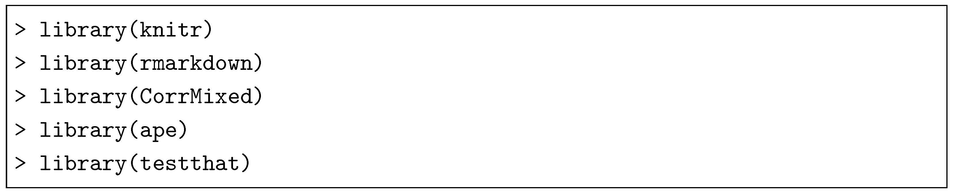
Appendix B.4. Imports and Suggests of R- Libraries

The following are the libraries required to run BSTZINB.

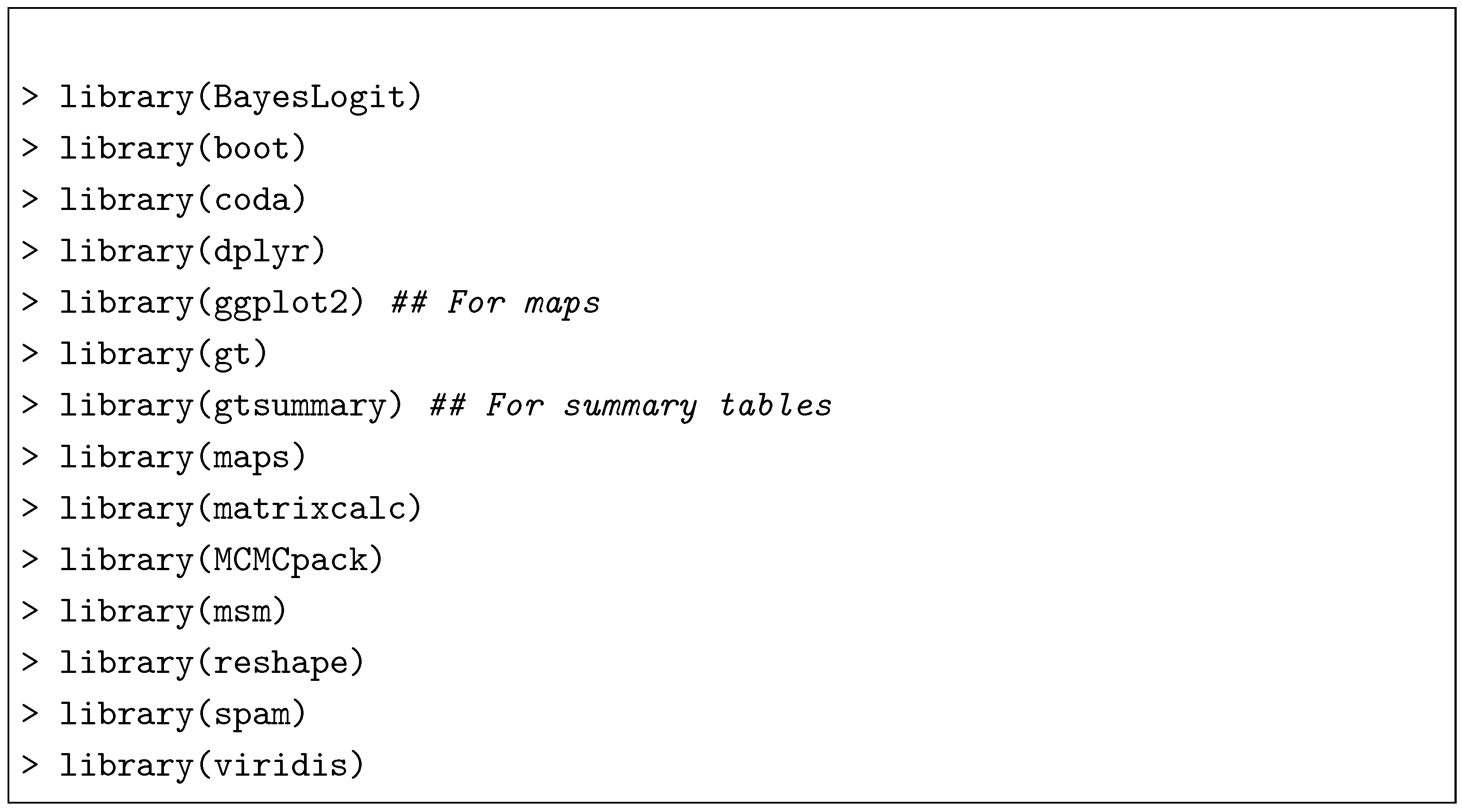
The following libraries are suggested for BSTZINB package:

References

- Chakraborty, S.; Dey, T.; Jun, Y.; Lim, C.Y.; Mukherjee, A.; Dominici, F. A spatiotemporal analytical outlook of the exposure to air pollution and COVID-19 mortality in the USA. J. Agric. Biol. Environ. Stat. 2022, 27, 419–439. [Google Scholar] [CrossRef] [Scilit]
- Yates, E.F.; Zhang, K.; Naus, A.; Forbes, C.; Wu, X.; Dey, T. A review on the biological, epidemiological, and statistical relevance of COVID-19 paired with air pollution. Environ. Adv. 2022, 8, 100250. [Google Scholar] [CrossRef] [Scilit]
- Dey, T.; Dominici, F. COVID-19, Air Pollution, and Racial Inequity: Connecting the Dots. Chem. Res. Toxicol. 2021, 34, 669–671. [Google Scholar] [CrossRef] [Scilit] [PubMed]
- Nicola, M.; Alsafi, Z.; Sohrabi, C.; Kerwan, A.; Al-Jabir, A.; Iosifidis, C.; Agha, M.; Agha, R. The socio-economic implications of the coronavirus pandemic (COVID-19): A review. Int. J. Surg. 2020, 78, 185–193. [Google Scholar] [CrossRef] [Scilit]
- Lambert, D. Zero-Inflated Poisson Regression, with an Application to Defects in Manufacturing. Technometrics 1992, 34, 1–14. [Google Scholar] [CrossRef] [Scilit]
- Min, Y.; Agresti, A. Random effect models for repeated measures of zero-inflated count data. Stat. Model. 2005, 5, 1–19. [Google Scholar] [CrossRef] [Scilit]
- Cameron, A.C.; Trivedi, P.K. Regression Analysis of Count Data, 2nd ed.; Econometric Society Monographs; Cambridge University Press: Cambridge, UK, 2013. [Google Scholar] [CrossRef] [Scilit]
- Hall, D.B. Zero-Inflated Poisson and Binomial Regression with Random Effects: A Case Study. Biometrics 2000, 56, 1030–1039. [Google Scholar] [CrossRef] [Scilit] [PubMed]
- Cameron, A.C.; Trivedi, P.K. Regression Analysis of Count Data; Cambridge University Press: Cambridge, UK, 1998. [Google Scholar] [CrossRef] [Scilit]
- Hilbe, J.M. Negative Binomial Regression, 2nd ed.; Cambridge University Press: Cambridge, UK, 2011. [Google Scholar] [CrossRef] [Scilit]
- Lawson, A.B. Bayesian Disease Mapping: Hierarchical Modeling in Spatial Epidemiology, 3rd ed.; CRC Press: Boca Raton, FL, USA, 2018. [Google Scholar]
- Banerjee, S.; Carlin, B.P.; Gelfand, A.E. Hierarchical Modeling and Analysis for Spatial Data, 2nd ed.; CRC Press: Boca Raton, FL, USA, 2015. [Google Scholar]
- Wakefield, J. Disease Mapping and Spatial Regression with Count Data. Biostatistics 2007, 8, 158–183. [Google Scholar] [CrossRef] [Scilit] [PubMed]
- Lee, D. CARBayes: An R Package for Bayesian Spatial Modeling with Conditional Autoregressive Priors. J. Stat. Softw. 2013, 55, 1–24. [Google Scholar] [CrossRef] [Scilit]
- Rue, H.; Martino, S.; Chopin, N. Approximate Bayesian Inference for Latent Gaussian Models by Using Integrated Nested Laplace Approximations. J. R. Stat. Soc. Ser. B Stat. Methodol. 2009, 71, 319–392. [Google Scholar] [CrossRef] [Scilit]
- He, Q.; Huang, H.H. A Framework of Zero-Inflated Bayesian Negative Binomial Regression Models for Spatiotemporal Data. J. Stat. Plan. Inference 2024, 229, 106098. [Google Scholar] [CrossRef] [Scilit]
- Neelon, B. Bayesian Zero-Inflated Negative Binomial Regression Based on Pólya-Gamma Mixtures. Bayesian Anal. 2019, 14, 829–855. [Google Scholar] [CrossRef] [Scilit] [PubMed]
- Gordon, W.J.; Riesenfeld, R.F. B-spline curves and surfaces. In Computer Aided Geometric Design; Elsevier: Amsterdam, The Netherlands, 1974; pp. 95–126. [Google Scholar]
- Polson, N.G.; Scott, J.G.; Windle, J. Bayesian Inference for Logistic Models Using Pólya–Gamma Latent Variables. J. Am. Stat. Assoc. 2013, 108, 1339–1349. [Google Scholar] [CrossRef] [Scilit]
- Pillow, J.; Scott, J. Fully Bayesian inference for neural models with negative-binomial spiking. In Advances in Neural Information Processing Systems; Bartlett, P., Pereira, F., Burges, C., Bottou, L., Weinberger, K., Eds.; MIT Press: Cambridge, MA, USA, 2012; Volume 25, pp. 1907–1915. [Google Scholar]
- Moran, P.A. Notes on continuous stochastic phenomena. Biometrika 1950, 37, 17–23. [Google Scholar] [CrossRef] [Scilit] [PubMed]
- Li, H.; Calder, C.A.; Cressie, N. Beyond Moran’s I: Testing for spatial dependence based on the spatial autoregressive model. Geogr. Anal. 2007, 39, 357–375. [Google Scholar] [CrossRef] [Scilit]
- Johnson, L.T.; Geyer, C.J. Variable transformation to obtain geometric ergodicity in the random-walk Metropolis algorithm. Ann. Stat. 2012, 40, 3050–3076. [Google Scholar] [CrossRef] [Scilit]
- Zhou, M.; Carin, L. Negative binomial process count and mixture modeling. IEEE Trans. Pattern Anal. Mach. Intell. 2013, 37, 307–320. [Google Scholar] [CrossRef] [Scilit]
- Geweke, J. Evaluating the Accuracy of Sampling-Based Approaches to the Calculation of Posterior Moments; Technical Report; Federal Reserve Bank of Minneapolis: Minneapolis, MN, USA, 1991. [Google Scholar]
- Geyer, C.J. Introduction to markov chain monte carlo. In Handbook of Markov Chain Monte Carlo; Routledge: London, UK, 2011; pp. 1–46. [Google Scholar]
- Gelman, A.; Carlin, J.B.; Stern, H.S.; Rubin, D.B. Bayesian Data Analysis; Chapman and Hall/CRC: Boca Raton, FL, USA, 1995. [Google Scholar]
- Spiegelhalter, D.J.; Best, N.G.; Carlin, B.P.; Van Der Linde, A. Bayesian measures of model complexity and fit. J. R. Stat. Soc. Ser. B Stat. Methodol. 2002, 64, 583–639. [Google Scholar] [CrossRef] [Scilit]
- Stan Development Team. RStan: The R Interface to Stan, R package version 2.32.6.; RStan: New York, NY, USA, 2024.
- Gelman, A.; Carlin, J.B.; Stern, H.S.; Dunson, D.B.; Vehtari, A.; Rubin, D.B. Bayesian Data Analysis; CRC Press: Boca Raton, FL, USA, 2013. [Google Scholar]
Disclaimer/Publisher’s Note: The statements, opinions and data contained in all publications are solely those of the individual author(s) and contributor(s) and not of MDPI and/or the editor(s). MDPI and/or the editor(s) disclaim responsibility for any injury to people or property resulting from any ideas, methods, instructions or products referred to in the content. |
© 2026 by the authors. Licensee MDPI, Basel, Switzerland. This article is an open access article distributed under the terms and conditions of the Creative Commons Attribution (CC BY) license.