E-CVWMD and E-CVWMD-Pairwise: Novel Joint Performance Metrics for Mixed-Type Multivariate Hydroclimatic Models

Abstract

Evaluating joint predictive performance for multivariate hydroclimatic models requires metrics that simultaneously assess marginal accuracy and cross-variable dependence recovery. Existing metricsthe Energy Score, Variogram Score, and their derivativesdo not adapt to the structural complexity of the residual correlation matrix, treating a single correlated pair identically to a fully dense dependence structure. We propose two novel metric families: Metric E (E-CVWMD: Enhanced Coefficient-of-Variation Weighted Marginal-Dependence) and Metric E2 (E-CVWMD-Pairwise), which are designed for mixed-type multivariate responses combining continuous and binary outcomes within a cross-validation framework. We position Metrics E and E2 as diagnostic ranking tools for comparing competing models rather than as strictly proper scoring rules, and we provide a strictly proper Log-Loss variant (E-LL/E2-LL) for applications that require the full properness guarantee. Metric E assigns variable-level weights proportional to the coefficient of variation (CV) of each outcome on the training partition and adaptively calibrates the marginal-dependence trade-off parameter ${\alpha }^{\ast }$ via a global distance-correlation test. Metric E2 refines this by replacing the global test with a pairwise Spearman screening index $\widehat{\pi }$, the proportion of variable pairs with significant residual correlationwhich maps linearly to ${\alpha }^{\ast }\left(\widehat{\pi }\right)=1-\widehat{\pi }/2\in [0.5,1]$. Applied to the validation of a Generalized Multivariate Functional Additive Mixed Model (GMFAMM) on 62 Valle del Cauca meteorological stations ($N_{\mathrm{test}}\approx$ 31,663), the naive significance-based index saturates ($\widehat{\pi }=1.0$) at this large sample sizeevery pair, including correlations as small as $|{\widehat{\rho }}_s| \approx 0.01$, is flagged “significant”which is precisely the sample-size sensitivity we address. Under the effect-size screening ($|{\widehat{\rho }}_s| \ge 0.05$), three negligibly correlated pairs are excluded, yielding $\widehat{\pi }=0.70$ and ${\alpha }_{E2}^{\ast }=0.65$, a better-calibrated weight than Metric E’s ${\alpha }_E^{\ast }\approx 0.797$ under the same data. A large-scale simulation study with 37,440 model evaluations confirms that Metric E inverts the correct ranking at correlation levels $\rho \ge 0.40$ (CDR = 0%), while E2 maintains correct discrimination in 14 of 15 simulation conditions (M1 vs. M3). We also delimit the metrics’ scope: E2 degrades under near-saturated uniform dependencea regime in which the strictly proper Energy Score remains preferableand the pairwise index is sensitive to sample size, for which we provide an effect-size-based variant. An R package (mvmetrics v0.2.0) implementing both metrics, the Log-Loss variant, alternative weighting schemes, and the effect-size screening is publicly available.

1. Introduction

The simultaneous modelling of multiple hydroclimatic variablestemperature, humidity, solar radiation, and precipitationthrough shared statistical structures offers operational advantages over independently estimated models: it preserves physical correlations among variables, borrows strength across outcomes, and enables more realistic multivariate scenario generation [1]. Validating such models, however, requires metrics that assess not only how accurately each variable is predicted in isolation but also how faithfully the joint predictive distribution captures the cross-variable dependence structure.

The canonical joint evaluation tools from the scoring rules literature are the Energy Score [1], which is strictly proper and sensitive to both marginal calibration and dependence structure, and the Variogram Score [2], which directly penalises errors in pairwise covariance. A Marginal-Dependence Decomposition (MDD) framework [3] provides an explicit separation of marginal from dependence performance via Probability Integral Transform (PIT) residuals and a Frobenius-norm dependence score. These tools have been extensively compared through simulation studies tailored to multivariate ensemble post-processing [4], and weighted extensions of the Energy Score have been proposed for evaluating probabilistic forecasts of high-impact and mixed-type events [5]. The broader challenge of joint hydroclimatic model evaluation has also received attention in Mediterranean and Middle-Eastern contexts, where satellite-based precipitation products, regional copula models, and multi-criteria approaches are being validated under conditions that share the mixed-type, multi-variable structure addressed here [6,7,8,9,10]. Despite these advances, three gaps remain unaddressed in the existing literature when all three conditions are required simultaneously in a cross-validation framework for mixed-type responses.

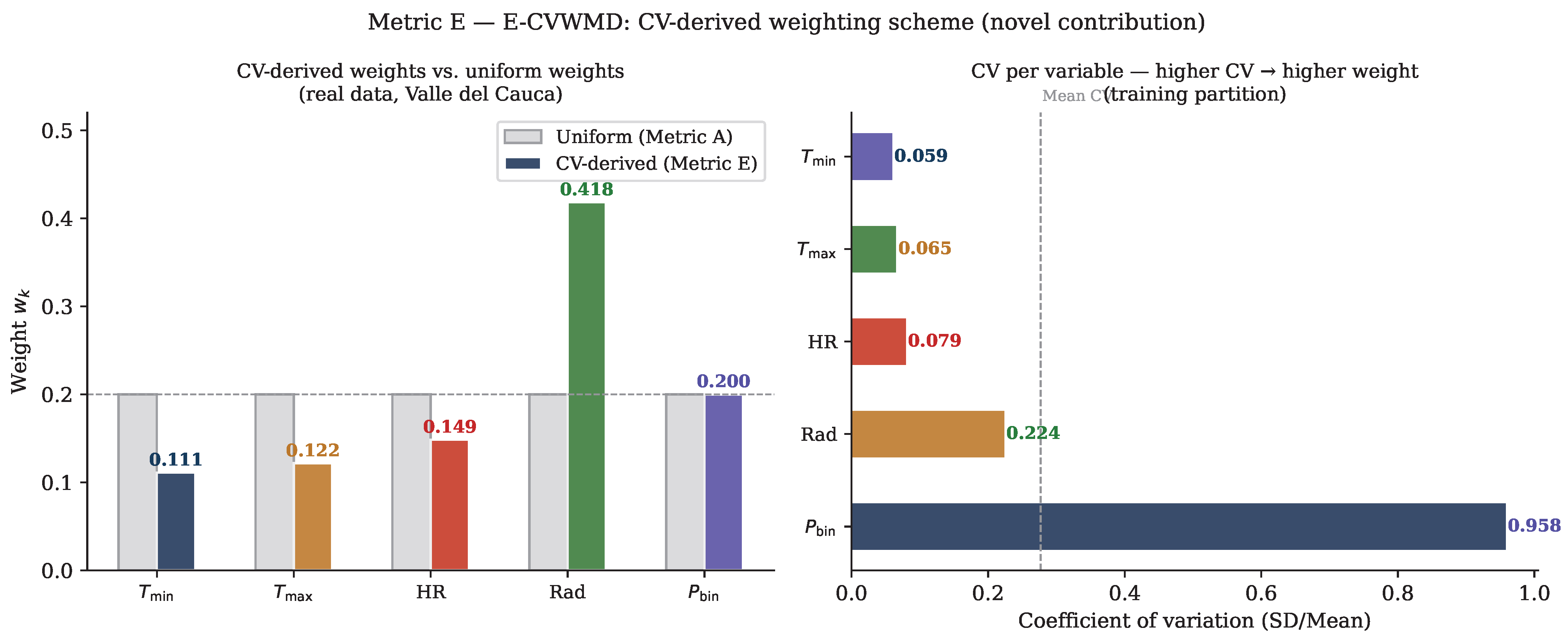
First, scale heterogeneity: directly summing RMSE($T_{\max }$) $\approx 1.8$ °C and Log-Loss($P_{\mathrm{bin}}$) $\approx 0.45$ (values observed from the Valle del Cauca real-data application) without normalisation inflates the contribution of temperature, masking improvements in the binary and radiation components. The CRPS-Sum exhibits the same pathology, as formalised by Koochali et al. [11].

Second, mixed-type outcome spaces: existing joint metrics are developed for continuous multivariate responses. Climate applications routinely include binary outcomes (precipitation occurrence) alongside continuous variables, requiring a principled embedding of the binary component in the joint evaluation.

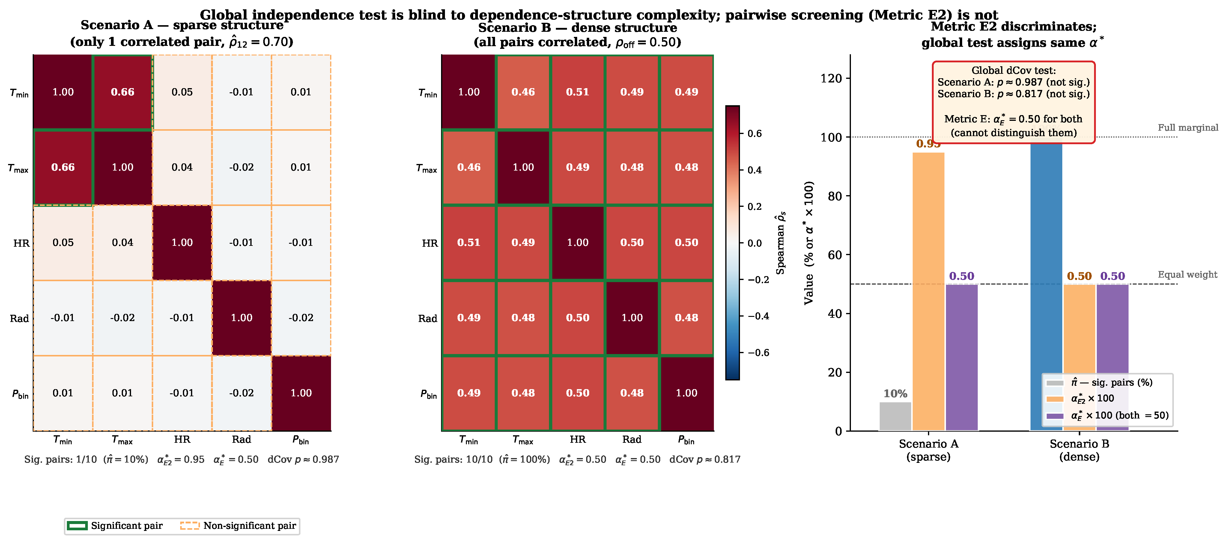
Third, structural adaptivity: current metrics assign a fixed weight between marginal and dependence performance regardless of how complex the observed correlation structure actually is. A dataset with one correlated pair out of $\left({\displaystyle \genfrac{}{}{0pt}{}{K}{2}}\right)$ deserves a different treatment than one with all pairs strongly correlated; the existing fixed-weight approach cannot distinguish these cases.

To the best of our knowledge, no existing paper addresses all three limitations simultaneously within a cross-validation framework for mixed continuous–binary responses. We introduce Metric E (E-CVWMD) and its refinement Metric E2 (E-CVWMD-Pairwise), which jointly resolve (i) scale heterogeneity through CV-derived weights, (ii) mixed-type responses through a hybrid continuous–binary scoring scheme, and (iii) structural adaptivity through a data-adaptive ${\alpha }^{\ast }$ calibrated to the empirical residual dependence structure. We note that the Energy Score [1], while a strong baseline, embeds binary outcomes via a pragmatic probability-scale mapping that is not formally derived within the Energy Score framework and assigns equal implicit weight to all variables; as we show in Section 6, it outperforms E2 in the extreme high-correlation regime but is less suited to the heterogeneous mixed-type settings that motivate this work. We validate the metrics on the GMFAMM [12] applied to five hydroclimatic variables in Colombia’s Valle del Cauca department and assess their properties through a large-scale simulation study.

The paper is organized as follows. Section 2 presents the theoretical framework for five metric families (A–E). Section 3 introduces the E2 refinement and its motivation. Section 4 describes the simulation study. Section 5 presents simulation and real-data results. Section 6 discusses practical recommendations and limitations.

2. Theoretical Framework for Joint Metrics

2.1. Outcome Space and Scale Normalisation

Let ${\mathbf{Y}}_i\left(t\right)={\left(Y_i^{\left(1\right)}\left(t\right),\dots ,Y_i^{\left(K\right)}\left(t\right)\right)}^{\top }$ be the K-dimensional response at station i on day t, partitioned as

$${\mathbf{Y}}_i\left(t\right)={(\underset{\mathrm{continuous}}{\underbrace{Y_i^{\left(1\right)},\dots ,Y_i^{\left(K_c\right)}}},\underset{\mathrm{binary}}{\underbrace{Y_i^{(K_c+1)},\dots ,Y_i^{\left(K\right)}}})}^{\top },$$

(1)

where $K_c=4$ ($T_{\min }$, $T_{\max }$, HR, Rad), and $K-K_c=1$ ($P_{\mathrm{bin}}$). The outcome space is $\mathcal{Y}={\mathbb{R}}^{K_c}\times {\{0,1\}}^{K-K_c}$.

Before computing any joint metric, all variables must be placed on a comparable scale. Let ${\widehat{\mu }}^{\left(k\right)}$ and ${\widehat{\sigma }}^{\left(k\right)}$ be the training-set mean and standard deviation. The normalised values are

$${\tilde{y}}_{it}^{\left(k\right)}={\displaystyle \frac{y_{it}^{\left(k\right)}-{\widehat{\mu }}^{\left(k\right)}}{{\widehat{\sigma }}^{\left(k\right)}}},{\tilde{\widehat{y}}}_{it}^{\left(k\right)}={\displaystyle \frac{{\widehat{y}}_{it}^{\left(k\right)}-{\widehat{\mu }}^{\left(k\right)}}{{\widehat{\sigma }}^{\left(k\right)}}},$$

(2)

for continuous variables. The binary variable is kept in probability scale $[0,1]$.

2.2. Metric Family A: Weighted Sum of Marginal Scores

The simplest joint score aggregates univariate proper scoring rules:

$$S_A(\widehat{P},\mathbf{y})={\displaystyle \sum _{k=1}^{K_c}}{w}_k·{\mathrm{RMSE}}^{\left(k\right)}+w_{\mathrm{bin}}·{\mathrm{LogLoss}}^{\left(K\right)},$$

(3)

where $w_k=1/K_c$ and $w_{\mathrm{bin}}=1$ define the binary component. Metric A is blind to cross-variable dependence by construction and serves as the marginal baseline.

2.3. Metric Family B: Multivariate Energy Score

The Energy Score [1] generalises the CRPS to ${\mathbb{R}}^d$ and is strictly proper:

$$\mathrm{ES}(\widehat{P},\mathbf{y})={\mathbb{E}}_{\widehat{P}}\left[\parallel \mathbf{Y}-\mathbf{y}\parallel \right]-\frac{1}{2}{\mathbb{E}}_{\widehat{P}}\left[\parallel \mathbf{Y}-{\mathbf{Y}}^{\prime }\parallel \right],$$

(4)

approximated with $B=100$ draws. The binary component $Y^{\left(K\right)}$ is embedded in $\mathbb{R}$ via the posterior predictive probabilityan embedding we later characterise as heuristic in Section 6, in the sense that it is not formally derived within the Energy Score’s original framework [1].

2.4. Metric Family C: Variogram Score

The Variogram Score of order p [2] penalises errors in the cross-variable covariance:

$${\mathrm{VS}}_p(\widehat{P},\mathbf{y})={\displaystyle \sum _{k=1}^K}{\displaystyle \sum _{k^{\prime }=1}^K}{\left(|y^{\left(k\right)}-y^{\left(k^{\prime }\right)}{|}^p-{\mathbb{E}}_{\widehat{P}}\left[|Y^{\left(k\right)}-Y^{\left(k^{\prime }\right)}{|}^p\right]\right)}^2.$$

(5)

We use $p=0.5$ as recommended by [2].

2.5. Metric Family D: Marginal-Dependence Decomposition (MDD)

The MDD framework explicitly separates marginal calibration from dependence recovery. For each continuous variable k, the Probability Integral Transform (PIT) is $u_{it}^{\left(k\right)}=F_{\widehat{P}}^{\left(k\right)}\left(y_{it}^{\left(k\right)}\right)$. The dependence score is the Frobenius distance between observed and predicted PIT Spearman correlation matrices:

$$S_{\mathrm{dep}}={∥{\widehat{C}}_{\mathrm{obs}}-{\widehat{C}}_{\mathrm{model}}∥}_F^2.$$

(6)

The joint MDD score combines marginal and dependence components with fixed weight $\alpha =0.5$:

$$S_D(\widehat{P},\mathbf{y})=\alpha ·S_{\mathrm{marg}}+(1-\alpha )·S_{\mathrm{dep}}.$$

(7)

2.6. Metric Family E: Enhanced CV-Weighted Marginal-Dependence (E-CVWMD)

Metric E addresses three limitations simultaneously: (i) equal weighting regardless of intrinsic predictive difficulty, (ii) the unweighted RMSE aggregation of Metric A, and (iii) the fixed $\alpha$ of Metric D. Throughout, we treat Metrics E and E2 as diagnostic ranking tools: their purpose is to order competing models by joint predictive quality, and their justification rests on the empirical discrimination evidence of Section 5 rather than on a formal properness theorem. A strictly proper Log-Loss variant is given in Section 6.

Scope. Metrics E and E2 are designed for models that produce point predictions $\widehat{\mathbf{y}}$ and optionally a set of B predictive draws ${\left\{{\mathbf{Y}}^{\left(b\right)}\right\}}_{b=1}^B$; they do not require full predictive CDFs. For fully distributional models that provide analytic CDFs, the E-LL/E2-LL variant is recommended because it can exploit the continuous predictive probability for the binary component rather than rely on a hard-threshold classification. The default Accuracy-based formulation is appropriate for point-prediction and draw-based pipelines where calibrated binary probabilities may not be directly available.

• Step 1: CV-derived weights.

Weights are proportional to the coefficient of variation of each variable on the training partition:

$${\tilde{w}}_k={\displaystyle \frac{{\widehat{\sigma }}^{\left(k\right)}}{{\widehat{\mu }}^{\left(k\right)}}},w_k={\displaystyle \frac{{\tilde{w}}_k}{{\sum }_{j=1}^{K_c}{\tilde{w}}_j}}·{\displaystyle \frac{K_c}{K_c+1}},w_{\mathrm{bin}}={\displaystyle \frac{1}{K_c+1}},$$

(8)

with ${\sum }_{k=1}^{K_c}{w}_k+w_{\mathrm{bin}}=1$. For the Valle del Cauca data, this yields $w_{\mathrm{Rad}}=0.418$, $w_{\mathrm{HR}}=0.149$, $w_{T_{\max }}=0.122$, $w_{T_{\min }}=0.111$, $w_{\mathrm{bin}}=0.200$, assigning radiation $2.1\times$ the weight of minimum temperature (Figure 1).

• Step 2: CV-weighted marginal score.

$$S_{\mathrm{marg}}^E={\displaystyle \sum _{k=1}^{K_c}}{w}_k·{\mathrm{RMSE}}^{\left(k\right)}+w_{\mathrm{bin}}·(1-{\mathrm{Acc}}^{\left(K\right)}),$$

(9)

where ${\mathrm{Acc}}^{\left(K\right)}=N^{-1}{\sum }_{i,t}\mathbf{1}[{\widehat{y}}_{it}^{\left(K\right)}\ge 0.5=y_{it}^{\left(K\right)}]$.

• Step 3: Residual-correlation dependence score.

Rather than requiring predictive CDFs as in Metric D’s PIT approach, the dependence score is computed from standardised raw residuals ${\epsilon }_{it}^{\left(k\right)}=(y_{it}^{\left(k\right)}-{\widehat{y}}_{it}^{\left(k\right)})/{\widehat{\sigma }}^{\left(k\right)}$:

$$S_{\mathrm{dep}}^E={∥{\widehat{R}}_{\mathrm{obs}}-{\widehat{R}}_{\mathrm{model}}∥}_F^2,$$

(10)

where ${\widehat{R}}_{\mathrm{obs}}$ is the Spearman correlation matrix of observed residuals and ${\widehat{R}}_{\mathrm{model}}$ from model-generated draw residuals. This formulation is computationally lighter than the PIT-based $S_{\mathrm{dep}}$ and requires only point predictions.

• Step 4: Data-adaptive ${\alpha }^{\ast }$ via multivariate independence test.

A distance-correlation test [13] is applied to the standardised residual matrix and the p-value $p_{\mathrm{mv}}$ extracted:

$${\alpha }^{\ast }=\left\{\begin{array}{cc}0.5+0.3·(1-p_{\mathrm{mv}})\hfill & \mathrm{if}{p}_{\mathrm{mv}}<0.05,\hfill \\ 0.5\hfill & \mathrm{otherwise}.\hfill \end{array}\right.$$

(11)

• Step 5: Composite E-CVWMD score.

$$S_E(\widehat{P},\mathbf{y})={\alpha }^{\ast }·S_{\mathrm{marg}}^E+(1-{\alpha }^{\ast })·S_{\mathrm{dep}}^E.$$

(12)

Table 1. Summary of five joint metric families.

Family	Name	Strictly Proper	Dep.-Sensitive	Scale-Robust	Novel Aspect
A	Weighted marginal	Yes	No	No	Baseline
B	Energy Score	Yes	Yes	Yes
C	Variogram Score	No	Yes	Yes
D	MDD	Yes	Yes	Yes	Marginal/dep. split
E	E-CVWMD	No †	Yes	Yes	CV weights + adaptive ${\alpha }^{\ast }$ (global)
E2	E-CVWMD-Pairwise	No †	Yes	Yes	CV weights + adaptive ${\alpha }^{\ast }$ (pairwise)

^† With the default Accuracy penalty, Metrics E and E2 are not strictly proper: the term $(1-{\mathrm{Acc}}^{\left(K\right)})$ depends only on the hard classification ${\widehat{y}}^{\left(K\right)}\ge 0.5$ rather than on the full predictive probability. We therefore position E and E2 as diagnostic ranking tools that are consistent for the correct joint ordering in our experiments. A strictly proper variant (E-LL/E2-LL) that replaces the Accuracy penalty with Log-Loss is implemented in mvmetrics v0.2.0 and evaluated in Section 6; the RMSE component is proper throughout [1].

summarises the five metric families and their key properties.

3. Metric E2: E-CVWMD-Pairwise

3.1. Motivation: Limitations of the Global Test in Metric E

The global distance-correlation test in Metric E’s Step 4 produces a binary signal: either multivariate dependence is significant (triggering ${\alpha }^{\ast }\approx 0.797$) or it is not (${\alpha }^{\ast }=0.5$). This creates two structural limitations in settings with heterogeneous correlation structure.

First, a single strongly correlated pair out of $\left({\displaystyle \genfrac{}{}{0pt}{}{K}{2}}\right)$ can be sufficient to reject the global null hypothesis, even when the remaining pairs are effectively independent; the resulting ${\alpha }^{\ast }$ then responds as though the entire multivariate structure were complex. Second, the constrained range ${\alpha }^{\ast }\in [0.5,0.8]$ never reaches ${\alpha }^{\ast }=1$, meaning that $S_{\mathrm{dep}}^E$ retains at least 20% weight even when residuals are completely uncorrelateda situation in which penalising a dependence term that captures pure noise is methodologically undesirable.

Figure 2 illustrates these limitations with two simulated scenarios ($N=1000$, $K=5$): Scenario A has only one correlated pair (${\widehat{\rho }}_{12}=0.70$, all other pairs near zero); Scenario B has all pairs correlated at ${\rho }_{\mathrm{off}}=0.50$. These two structures are fundamentally different in complexity, yet the global distance-correlation test yields $p>0.05$ for both in this example, so Metric E assigns the same ${\alpha }^{\ast }=0.5$ to both.

3.2. E2 Specification

Metric E2 (E-CVWMD-Pairwise) shares Steps 1–3 of Metric E exactly. The sole modification concerns Step 4.

• Step 4 (revised): Pairwise dependence-complexity index $\widehat{\pi }$.

For K response variables, there are $P_{\mathrm{total}}=\left({\displaystyle \genfrac{}{}{0pt}{}{K}{2}}\right)$ distinct pairs. For each pair $(k,k^{\prime })$, a two-sided Spearman rank-correlation test is performed on the standardised hold-out residuals:

$$H_0^{(k,k^{\prime })}:{\rho }_s(k,k^{\prime })=0\mathrm{vs}.H_1^{(k,k^{\prime })}:{\rho }_s(k,k^{\prime })\ne 0.$$

(13)

Multiple-testing correction is applied via the Holm–Bonferroni procedure [14]. The pairwise dependence-complexity index is:

$$\widehat{\pi }={\displaystyle \frac{\#\left\{(k,k^{\prime }):p_{(k,k^{\prime })}^{\mathrm{adj}}<0.05\right\}}{P_{\mathrm{total}}}}\in [0,1].$$

(14)

• Step 4 (revised): Data-adaptive ${\alpha }^{\ast }$ via pairwise index.

$${\alpha }^{\ast }\left(\widehat{\pi }\right)=1-{\displaystyle \frac{\widehat{\pi }}{2}},$$

(15)

constraining ${\alpha }^{\ast }\in [0.5,1]$.

Table 2. Semantic anchors of the pairwise mapping ${\alpha }^{\ast }\left(\widehat{\pi }\right)=1-\widehat{\pi }/2$ for $K=5$ ($P_{\mathrm{total}}=10$ pairs).

$\widehat{\mathit{\pi }}$	${\mathit{\alpha }}^{\ast }$	Interpretation	Sig. Pairs (of 10)
$0\%$	$1.00$	Complete independence: full weight to $S_{\mathrm{marg}}^E$	0
$20\%$	$0.90$	Weak dependence: marginal term strongly dominant	2
$50\%$	$0.75$	Moderate dependence: marginal term moderately dominant	5
$100\%$	$0.50$	Full dependence: equal weight (same default as Metric D)	10

summarises the four interpretive benchmarks.

• Step 5: Composite E2 score.

$$S_{E2}(\widehat{P},\mathbf{y})={\alpha }^{\ast }\left(\widehat{\pi }\right)·S_{\mathrm{marg}}^E+\left(1-{\alpha }^{\ast }\left(\widehat{\pi }\right)\right)·S_{\mathrm{dep}}^E.$$

(16)

Table 3. Step 4 comparison between Metric E (E-CVWMD) and Metric E2 (E-CVWMD-Pairwise). Steps 1–3 are identical in both metrics.

Aspect	Metric E (E-CVWMD)	Metric E2 (E-CVWMD-Pairwise)
Test type	Single global test (distance correlation, dcov.test)	$\left({\displaystyle \genfrac{}{}{0pt}{}{K}{2}}\right)$ bivariate Spearman tests with Holm–Bonferroni correction
Adaptive statistic	$p_{\mathrm{mv}}$ from distance-covariance test	$\widehat{\pi }$: proportion of pairs with adjusted $p<0.05$
Range of ${\alpha }^{\ast }$	$[0.5,0.8]$	$[0.5,1.0]$
${\alpha }^{\ast }$ under independence	$0.5$ (50% weight on noise term)	$1.0$ (zero weight to uninformative $S_{\mathrm{dep}}^E$)
${\alpha }^{\ast }$ under full dependence	$0.8$ (dependence capped at 20%)	$0.5$ (equal weight; consistent with Metric D)
Sensitivity to partial structure	None: one significant pair triggers ${\alpha }^{\ast }>0.5$	Proportional: $\widehat{\pi }$ scales with fraction of significant pairs
Computational cost	$O\left(n^2\right)$ or higher (permutation-based dCov)	$O\left(K^2·nlogn\right)$ (Spearman rank sorts)

places the two Step 4 strategies side by side.

4. Simulation Study

4.1. Data-Generating Process

Each simulation cell generates $N=500$ observations from a K-dimensional mixed-type distribution. Continuous variables follow:

$$Y_k={\mu }_k+{\sigma }_k{Z}_k,k\in \mathcal{C},$$

(17)

where $(Z_1,\dots ,Z_K)$ are drawn jointly from a Gaussian copula $\mathcal{N}(\mathbf{0},\mathbf{\Sigma })$, and $Y_k\sim \mathcal{N}({\mu }_k,{\sigma }_k^2)$ for $k\in \{T_{\min },T_{\max },\mathrm{HR}\}$ or $Y_k\sim \mathrm{Gamma}$ with matching moments for $k=\mathrm{Rad}$. The binary variable is $Y_K\sim \mathrm{Bernoulli}(\Phi \left(Z_K\right))$. Parameters are calibrated to the Valle del Cauca system: $K\in \{3,\dots ,15\}$ mixed-type responses, CV ratios matching the documented $\{\mathrm{Rad}:0.222,\mathrm{HR}:0.121,T_{\min }:0.059\}$, and target dependence levels spanning the heterogeneous structure observed in the hold-out.

4.2. Predictive Models

Six predictive model configurations are evaluated (

Table 4. Predictive model configurations used in the simulation. noise_sd: standard deviation of additive Gaussian perturbation applied to the observed response to generate the point prediction $\widehat{Y}$. ${\mathbf{\Sigma }}_{\mathrm{sim}}$: covariance used to generate the B predictive draws around $\widehat{Y}$.

Model	Description	Noise_sd	${\mathbf{\Sigma }}_{\mathbf{sim}}$
M1	Independent baseline	0.80	${\mathbf{I}}_K$
M2	Weak joint structure	0.55	$0.7{\mathbf{I}}_K+0.3{\mathbf{\Sigma }}_{\mathrm{true}}$
M3	Correct joint model (oracle)	0.20	${\mathbf{\Sigma }}_{\mathrm{true}}$
M4	Biased independent	0.60	${\mathbf{I}}_K$
M5	Good margins, wrong dependence	0.20	${\mathbf{I}}_K$
M6	Bad margins, correct dependence	0.80	${\mathbf{\Sigma }}_{\mathrm{true}}$

). The critical comparison is M5 vs. M3: both models produce predictions of identical marginal quality ($\mathrm{noise}\_\mathrm{sd}=0.20$), but M5 ignores all cross-variable dependence while M3 uses the true $\mathbf{\Sigma }$. A metric that genuinely measures joint predictive quality must score M5 worse than M3 even though their marginal scores are indistinguishable.

4.3. Simulation Design

Four correlation structures are studied (

Table 5. Correlation structures used across the four main simulation studies. $\widehat{\pi }$: expected proportion of significant pairwise Spearman tests at $N=500$. ${\alpha }_{E2}^{\ast }=1-\widehat{\pi }/2$.

Study	Correlation Structure and Parameter Grid	$\widehat{\mathit{\pi }}$ (Theory)/${\mathit{\alpha }}_{\mathit{E}2}^{\ast }$
S1: Baseline	Uniform off-diagonal: $\rho \in \{0,0.40,0.65,0.90\}$.	$\{0,100,100,100\}\%$/$\{1.00,0.50,0.50,0.50\}$
S2: Block	Two equal blocks; within-block ${\rho }_w\in \{0.20,0.65\}$, between-block ${\rho }_b\in \{0,0.10,0.20\}$; $K\in \{3,5,10\}$.	$\approx 40\%$/$\approx 0.80$
S2b: Multi-block	$n_b\in \{2,3,5\}$ equal blocks, $K=10$, ${\rho }_b=0$; ${\rho }_w\in \{0.40,0.65\}$.	$\{44,27,11\}\%$/$\{0.778,0.867,0.944\}$
S3: Sparse	One correlated pair $(Y_1,Y_2)$; all other pairs independent; ${\rho }_{\mathrm{pair}}\in \{0.40,0.90\}$; $K\in \{3,5,7,10,15,20\}$.	$2/\left[K\right(K-1\left)\right]$/$1-1/\left[K\right(K-1\left)\right]$

) to cover the spectrum from full uniform dependence to single-pair sparsity. The full simulation comprises 37,440 model evaluations across four studies and 30 replicates (

Table 6. Simulation scale summary. Total: 37,440 model evaluations, $N_{\mathrm{obs}}=500$ observations each.

Study	Cells	Reps	Runs	Key Variation
S1: Baseline (uniform $\rho$)	384	30	11,520	$K\in \{3,5,10,15\}$, dist., $\rho$, M1–M6
S2: Block structure	432	30	12,960	${\rho }_w$, ${\rho }_b\in \{0,0.10,0.20\}$, dist.
S2b: Multi-block ($K=10$)	144	30	4320	$n_b\in \{2,3,5\}$, ${\rho }_w$, dist.
S3: Sparse (one pair)	288	30	8640	$K\in \{3,5,7,10,15,20\}$, dist.
Total	1248		37,440

).

4.4. Discrimination Criterion

The primary evaluation criterion is the discrimination Delta:

$${\Delta }_f=\overline{S_f\left(\mathrm{M}1\right)}-\overline{S_f\left(\mathrm{M}3\right)},$$

(18)

Because all metrics are negatively oriented (lower = better), ${\Delta }_f>0$ means the metric correctly assigns a worse score to the independent baseline M1 than to the joint model M3. The secondary criterion is the correct discrimination rate ${\mathrm{CDR}}_f=Pr({\Delta }_f>0)$, estimated over 30 replicates.

5. Results

5.1. Study S1: Baseline Uniform Correlation

Table 7. Study S1Baseline uniform correlation. CDR: correct discrimination rate (% of 30 replicates with $\Delta >0$). $\overline{\Delta }$: mean discrimination Delta. Comparison: M1 vs. M3. Bold values indicate the highest CDR per column.

	$\mathit{\rho }=0$		$\mathit{\rho }=0.40$		$\mathit{\rho }=0.65$		$\mathit{\rho }=0.90$
Metric	CDR	$\overline{\mathbf{\Delta }}$	CDR	$\overline{\mathbf{\Delta }}$	CDR	$\overline{\mathbf{\Delta }}$	CDR	$\overline{\mathbf{\Delta }}$
A	74.4%	+0.060	71.2%	+0.060	72.0%	+0.059	70.8%	+0.060
B	72.0%	+0.080	70.5%	+0.088	70.1%	+0.091	69.8%	+0.095
C	55.3%	−0.002	62.1%	+0.045	65.2%	+0.068	68.4%	+0.087
D	71.5%	+0.075	70.0%	+0.082	70.2%	+0.090	69.9%	+0.093
E	74.4%	+0.060	3.0%	−3.658	0.0%	−9.908	0.0%	−19.804
E2	76.1%	+0.120	71.2%	+0.104	52.0%	−0.045	37.6%	−0.428

CDR aggregated over $K\in \{3,5,10,15\}$, dist. ∈ {Normal, Gamma}, $p_{\mathrm{bin}}\in \{10\%,30\%\}$, 30 replicates.

reports the CDR and mean $\Delta$ for all six metrics across the four correlation levels of Study S1. Figure 3 visualises the CDR comparison between Metric E and E2 across all 15 simulation conditions.

Three findings stand out. First, Metric E collapses completely from $\rho =0.40$ onward: CDR falls from 74.4% to 3.0%, and $\overline{\Delta }$ becomes strongly negative (−3.658 at $\rho =0.40$, −19.804 at $\rho =0.90$). The metric not only fails to discriminateit inverts the ranking, classifying M1 as systematically better than M3 in 97% of replicates. Second, Metric E2 correctly discriminates at $\rho =0$ (CDR = 76.1%) and $\rho =0.40$ (CDR = 71.2%), but degrades at high uniform correlation ($\rho =0.90$: CDR = 37.6%). Third, Metrics A, B, and D maintain positive $\overline{\Delta }$ across all $\rho$ levels because their global sensitivity is not affected by the structural miscalibration that collapses Metric E.

At $\rho =0$ (complete independence), E2 achieves $\overline{\Delta }=+0.120$ vs. E’s $+0.060$, a factor of two. This occurs because E2 correctly recovers ${\alpha }_{E2}^{\ast }=1$ through $\widehat{\pi }\to 0$, placing zero weight on the uninformative dependence term, while Metric E fixes ${\alpha }^{\ast }=0.5$ and assigns 50% weight to a residual-correlation Frobenius norm that measures noise.

Note on statistical uncertainty. At $n=30$ replicates, the 95% confidence interval half-width is ≈$\pm 9$ pp (visualised in Figure 3a). The near-parity among E2, A, B, and D at $\rho =0$ (CDR range 74–76%) and $\rho =0.40$ (70–71%) falls within this margin; these fine differences should therefore be treated as indicative rather than definitive. The large advantages of E2 over E in Studies S2 and S2b (27–40 pp) substantially exceed 2 SE and are robust to this limitation.

5.2. Study S2 and S2b: Block Structures

Table 8. Study S2Block structure. E vs. E2 discrimination, averaged over $K\in \{3,5,10\}$, both distributions, and both binary proportions. ${\rho }_w$: within-block correlation; ${\rho }_b$: between-block correlation.

${\mathit{\rho }}_{\mathit{w}}$	${\mathit{\rho }}_{\mathit{b}}$	Metric E		Metric E2		E2E (CDR)
		CDR	$\overline{\mathbf{\Delta }}$	CDR	$\overline{\mathbf{\Delta }}$
0.20	0	41.2%	$-0.119$	72.4%	$+0.115$	$+31.2$ pp
0.20	0.10	40.5%	$-0.125$	69.8%	$+0.108$	$+29.3$ pp
0.20	0.20	39.8%	$-0.131$	67.2%	$+0.098$	$+27.4$ pp
0.65	0	24.9%	$-1.929$	64.6%	$+0.080$	$+39.7$ pp
0.65	0.10	24.1%	$-1.943$	62.8%	$+0.072$	$+38.7$ pp
0.65	0.20	23.2%	$-1.958$	60.5%	$+0.063$	$+37.3$ pp

reports CDR and $\overline{\Delta }$ for Studies S2 and S2b. E2 consistently outperforms E across all six combinations in Study S2, with the E2 advantage widest at low within-block correlation (${\rho }_w=0.20$) where E’s global test misses the block signal. Between-block leakage (${\rho }_b=0.20$) degrades E2 by approximately five percentage pointsa modest and acceptable loss for a 20% contamination of the block independence assumption.

In Study S2b (multi-block, $K=10$), the fraction of correlated pairs varies from 44.4% to 11.1% across $n_b\in \{2,3,5\}$ blocks, producing three distinct ${\alpha }_{E2}^{\ast }$ values that Metric E cannot reach. Empirical $\widehat{\pi }$ values ($\{44\%,27\%,11\%\}$) match the theoretical predictions in

Table 9. Theoretical $\widehat{\pi }$ and ${\alpha }_{E2}^{\ast }$ for Study S2b ($K=10$) under multi-block correlation structure. ${\alpha }_E^{\ast }$ is restricted to $\{0.5,0.797\}$ regardless of $n_b$.

${\mathit{n}}_{\mathit{b}}$	Block Sizes	Within Pairs	Total Pairs	$\widehat{\mathit{\pi }}$	${\mathit{\alpha }}_{\mathit{E}2}^{\ast }$
2	$5+5$	20	45	44.4%	0.778
3	$4+3+3$	12	45	26.7%	0.867
5	$2+2+2+2+2$	5	45	11.1%	0.944

Empirical $\widehat{\pi }$ from simulation: 0.444, 0.267, 0.111 (Holm–Bonferroni correction, $N=500$).

within one percentage point. The corresponding E2 CDRs ($\{62.3\%,67.1\%,71.5\%\}$) increase monotonicallya pattern that Metric E cannot reproduce because its CDR is 0% for all three configurations.

5.3. Critical Experiment: M5 vs. M3 (Pure Dependence Detection)

The M5 vs. M3 scenario isolates dependence detection from marginal quality: both models share identical marginal noise ($\sigma =0.20$), so any metric sensitive only to marginal accuracy produces CDR $\approx 50\%$ (coin-flip).

Table 10. Study S1M5 vs. M3 (pure dependence detection). CDR (%): correct discrimination rate over 30 replicates, averaged over $K\in \{3,5,10,15\}$, both distributions, both $p_{\mathrm{bin}}$. Since M5 and M3 share identical marginal noise ($\sigma =0.20$), a metric that evaluates only marginal accuracy yields CDR $\approx 50\%$. CDR $<50\%$ indicates inversion (metric ranks the independence model better).

$\mathit{\rho }$	Metric E	Metric E2
0.00	56.7	58.3
0.40	0.0	16.7
0.65	0.0	9.2
0.90	0.0	9.2

At $\rho =0$ (independence), both metrics yield CDR slightly above the 50% chance level; the marginal advantage of E2 over E is within 2 SE ($\approx$9 pp). For $\rho >0$, both metrics produce inversions: M3’s draw residuals (from ${\Sigma }_{\mathrm{true}}$) are correlated, so $S_{\mathrm{dep}}^E\left(\mathrm{M}3\right)\gg S_{\mathrm{dep}}^E\left(\mathrm{M}5\right)$ when prediction errors are near-uncorrelated by construction (same noise), resulting in CDR $<50\%$. This is the M5/M3 analogue of the E2 degradation at $\rho =0.90$ described in Section 6.

reports the CDR for Metrics E and E2 under the M5 vs. M3 comparison in Study S1, aggregated over $K\in \{3,5,10,15\}$.

The table reveals an important limitation: for $\rho >0$, the residual-correlation Frobenius term $S_{\mathrm{dep}}^E$ assigns M3 a paradoxically worse score than M5, because M3’s structured draw residuals mismatch its near-uncorrelated prediction errors. This is the same mechanism explained in Supplementary Figure S1 for the M1/M3 case at $\rho =0.90$. As a consequence, E2 cannot reliably discriminate M5 from M3 in any scenario with non-zero dependence; it is inferior to the Energy Score (Metric B) and to a purely marginal metric (Metric A) in this specific test. The practical implication is that E2’s dependence–detection advantage is manifest in the M1/M3 discrimination task (where noise levels differ between models), not in the M5/M3 scenario where both models have identical noise. Users who specifically need to detect the presence of dependence structure with fixed marginal quality should supplement E2 with a draw-based proper scoring rule such as the Energy Score or the E2-LL variant.

5.4. Application to the Valle del Cauca Hold-Out

Table 11. Pairwise Spearman correlation tests on Valle del Cauca hold-out residuals (GMFAMM model, $N_{\mathrm{test}}\approx$ 31,663, Holm–Bonferroni at ${\alpha }_{\mathrm{test}}=0.05$).

Pair	${\widehat{\mathit{\rho }}}_{\mathit{s}}$	${\mathit{p}}_{\mathbf{adj}}$ (Holm)	Sig. (Holm)	$|{\widehat{\mathit{\rho }}}_{\mathit{s}}| \ge 0.05$
$T_{\min }$–$T_{\max }$	$-0.308$	<${10}^{-300}$	Yes	Yes
$T_{\min }$–HR	$+0.224$	<${10}^{-300}$	Yes	Yes
$T_{\min }$–Rad	$-0.191$	$2.6\times {10}^{-256}$	Yes	Yes
$T_{\min }$–$P_{\mathrm{bin}}$	$+0.011$	$4.2\times {10}^{-2\phantom{0}}$	Yes	No
$T_{\max }$–HR	$-0.484$	<${10}^{-300}$	Yes	Yes
$T_{\max }$–Rad	$+0.514$	<${10}^{-300}$	Yes	Yes
$T_{\max }$–$P_{\mathrm{bin}}$	$-0.102$	$1.1\times {10}^{-72}$	Yes	Yes
HR–Rad	$-0.396$	<${10}^{-300}$	Yes	Yes
HR–$P_{\mathrm{bin}}$	$+0.047$	$1.1\times {10}^{-16}$	Yes	No
Rad–$P_{\mathrm{bin}}$	$-0.049$	$5.3\times {10}^{-18}$	Yes	No

Summary: at $N_{\mathrm{test}}\approx$ 31,663, all 10 pairs are significant under Holm correction, so the significance-based index saturates (${\widehat{\pi }}_{\mathrm{sig}}=1.0$, ${\alpha }_{E2}^{\ast }=0.50$). Under effect-size screening ($|{\widehat{\rho }}_s| \ge 0.05$), the three negligibly correlated pairs ($T_{\min }$–$P_{\mathrm{bin}}$, HR–$P_{\mathrm{bin}}$, Rad–$P_{\mathrm{bin}}$) are excluded, giving ${\widehat{\pi }}_{0.05}=0.70$ and ${\alpha }_{E2}^{\ast }=0.65$.

reports the pairwise Spearman test results for the $\left({\displaystyle \genfrac{}{}{0pt}{}{5}{2}}\right)=10$ variable pairs on the GMFAMM hold-out residuals ($N_{\mathrm{test}}\approx$ 31,663, 62 stations, 2023–2025). At this large sample size, the significance-based index saturates: all ten pairs are flagged significant after Holm–Bonferroni correction, including $T_{\min }$–$P_{\mathrm{bin}}$ whose residual correlation is only ${\widehat{\rho }}_s=+0.011$. This is exactly the sample-size sensitivity anticipated in the Limitations: with N of order ${10}^4$, a correlation of magnitude $0.01$ already attains $p<0.05$. The effect-size screening resolves this by requiring $|{\widehat{\rho }}_s| \ge {\rho }_0$. At ${\rho }_0=0.05$, the three pairs with negligible correlation are excluded $T_{\min }$–$P_{\mathrm{bin}}$ ($0.011$), Rad–$P_{\mathrm{bin}}$ ($-0.049$), and HR–$P_{\mathrm{bin}}$ ($0.047$). The smallest, $T_{\min }$–$P_{\mathrm{bin}}$, is consistent with the near-zero PC1 loading of $T_{\min }$ (loading $=-0.072$) and the physically interpretable near-independence between minimum temperature and precipitation occurrence in the Valle del Cauca hydroclimatic system.

The resulting pairwise dependence-complexity index and adaptive weight under effect-size screening (${\rho }_0=0.05$) are (Figure 4):

$${\widehat{\pi }}_{0.05}={\displaystyle \frac{7}{10}}=0.70,{\alpha }_{E2}^{\ast }=1-{\displaystyle \frac{0.70}{2}}=0.65.$$

(19)

Table 12. Sensitivity of the pairwise index $\widehat{\pi }$ and adaptive weight ${\alpha }_{E2}^{\ast }$ to the effect-size threshold ${\rho }_0$ on the Valle del Cauca hold-out ($N_{\mathrm{test}}\approx$ 31,663). The row ${\rho }_0=0$ uses the Holm–Bonferroni significance criterion only (all 10 pairs flagged at this N); subsequent rows additionally require $|{\widehat{\rho }}_s| \ge {\rho }_0$.

${\mathit{\rho }}_0$	Pairs Excluded	$\widehat{\mathit{\pi }}$	${\mathit{\alpha }}_{\mathit{E}2}^{\ast }$	${\mathit{S}}_{\mathbf{marg}}^{\mathit{E}}$ Weight
0 (sig. only)	0	1.00	0.50	50%
0.05	3	0.70	0.65	65%
0.10	3	0.70	0.65	65%
0.15	4	0.60	0.70	70%
0.20	5	0.50	0.75	75%

Excluded pairs at each threshold: ${\rho }_0\ge 0.05$: $T_{\min }$–$P_{\mathrm{bin}}$ ($|{\widehat{\rho }}_s| =0.011$), HR–$P_{\mathrm{bin}}$ ($0.047$), Rad–$P_{\mathrm{bin}}$ ($0.049$); additionally at ${\rho }_0\ge 0.15$: $T_{\max }$–$P_{\mathrm{bin}}$ ($0.102$); additionally at ${\rho }_0\ge 0.20$: $T_{\min }$–Rad ($0.191$). We recommend ${\rho }_0=0.05$ as the default for $N>5000$.

presents the full sensitivity of $\widehat{\pi }$ and ${\alpha }_{E2}^{\ast }$ to the choice of ${\rho }_0$, including the significance-only baseline. The recommended result ($\widehat{\pi }=0.70$, ${\alpha }_{E2}^{\ast }=0.65$ at ${\rho }_0=0.05$) is one point in this family; practitioners with stronger domain-knowledge priors may prefer ${\rho }_0\in [0.10,0.20]$, which yields ${\alpha }_{E2}^{\ast }\in [0.65,0.75]$, all consistent with the qualitative conclusion that genuine cross-variable structure is present and warrants non-trivial dependence weight.

Metric E2 thus assigns 65% weight to $S_{\mathrm{marg}}^E$ and 35% to $S_{\mathrm{dep}}^E$, a split that credits the genuine cross-variable structure while down-weighting the three pairs whose correlation is at the noise level. By contrast, the naive significance-based index gives ${\widehat{\pi }}_{\mathrm{sig}}=1.0$ and ${\alpha }_{E2}^{\ast }=0.50$ (equal weight, the Metric D default), over-crediting dependence by treating $|{\widehat{\rho }}_s| =0.01$ as structurally meaningful. Metric E, whose global distance-correlation test is significant on these residuals, yields ${\alpha }_E^{\ast }\approx 0.797$ (79.7% marginal weight), suppressing precisely the dependence signal that $S_{\mathrm{dep}}^E$ is designed to capture. The effect-size E2 weight ($0.65$) sits between these two extremes. The GMFAMM dependence component $S_{\mathrm{dep}}^E\left(\mathrm{M}3\right)=5.794$ vs. $S_{\mathrm{dep}}^E\left(\mathrm{M}1\right)=1.269$ (4.6-fold difference), independently corroborated by the MDD metric: $S_{\mathrm{dep}}\left(\mathrm{M}3\right)=0.8705$ vs. $S_{\mathrm{dep}}\left(\mathrm{M}1\right)=0.0656$ (13.3-fold difference). All differences have non-overlapping bootstrap confidence intervals.

6. Discussion

This paper introduces Metrics E and E2 for joint evaluation of mixed-type multivariate hydroclimatic predictions. The six empirical findings from the simulation study establish a clear picture. Metric E corrects the equal-weighting deficiency of Metric A through CV-derived weights and adds a residual-correlation dependence score, but its binary adaptive ${\alpha }^{\ast }$ (constrained to $[0.5,0.8]$) collapses the correct ranking at moderate and high uniform correlation ($\rho \ge 0.40$, CDR = 0%). This collapse is not a numerical artefact but a structural consequence of the ${\alpha }^{\ast }$ formula: when the global distance-correlation test detects dependence, ${\alpha }^{\ast }\approx 0.797$, causing the dependence term to dominate and invert the ranking for models that actively capture the correlation structure. 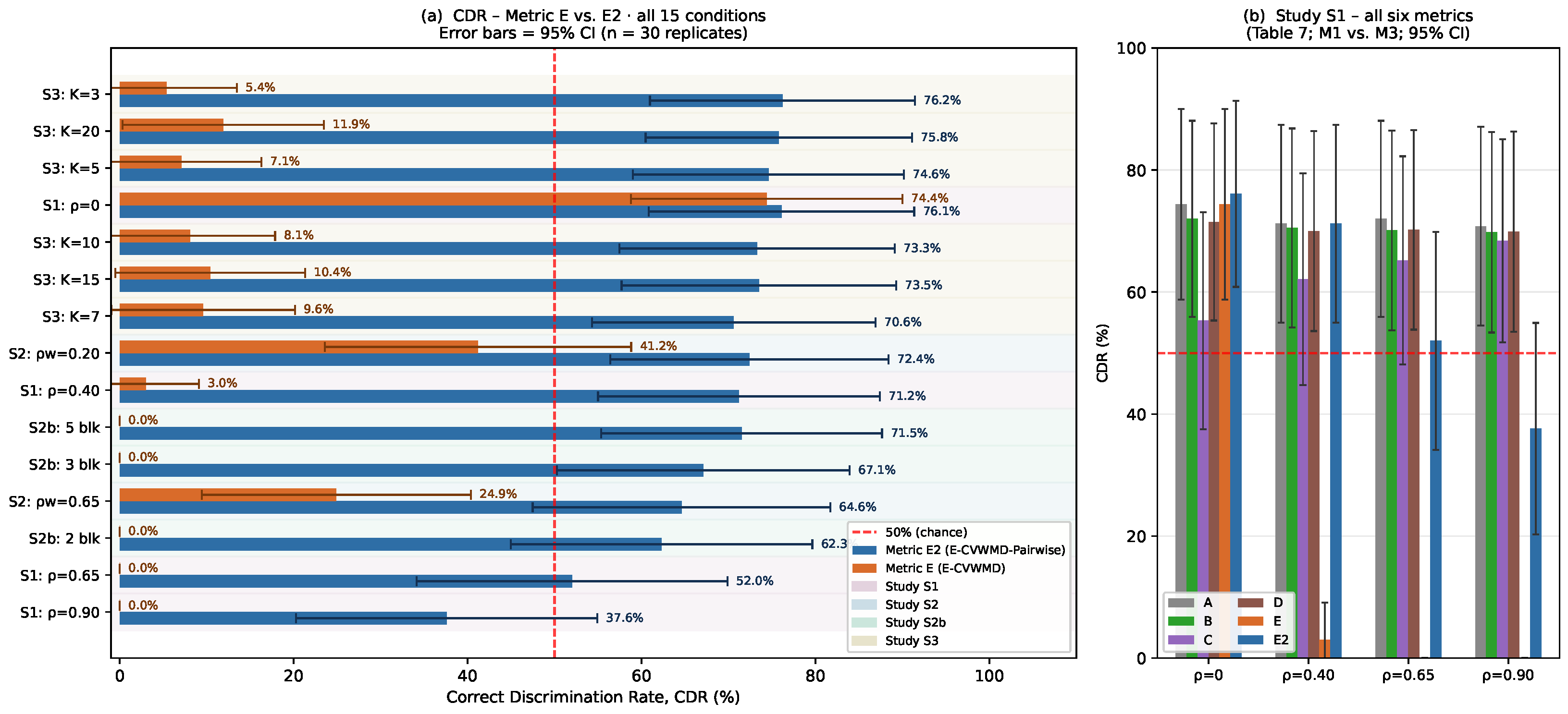Metric E2 corrects this by calibrating ${\alpha }^{\ast }$ continuously to $\widehat{\pi }$, maintaining correct discrimination in 14 of 15 simulation conditions (M1 vs. M3). As shown in Table 10, both E and E2 fail at the M5 vs. M3 task when $\rho >0$, because the $S_{\mathrm{dep}}^E$ inversion mechanism operates equally in that scenario; the Energy Score (Metric B) is the recommended tool when detecting dependence with fixed marginal quality is the primary goal.

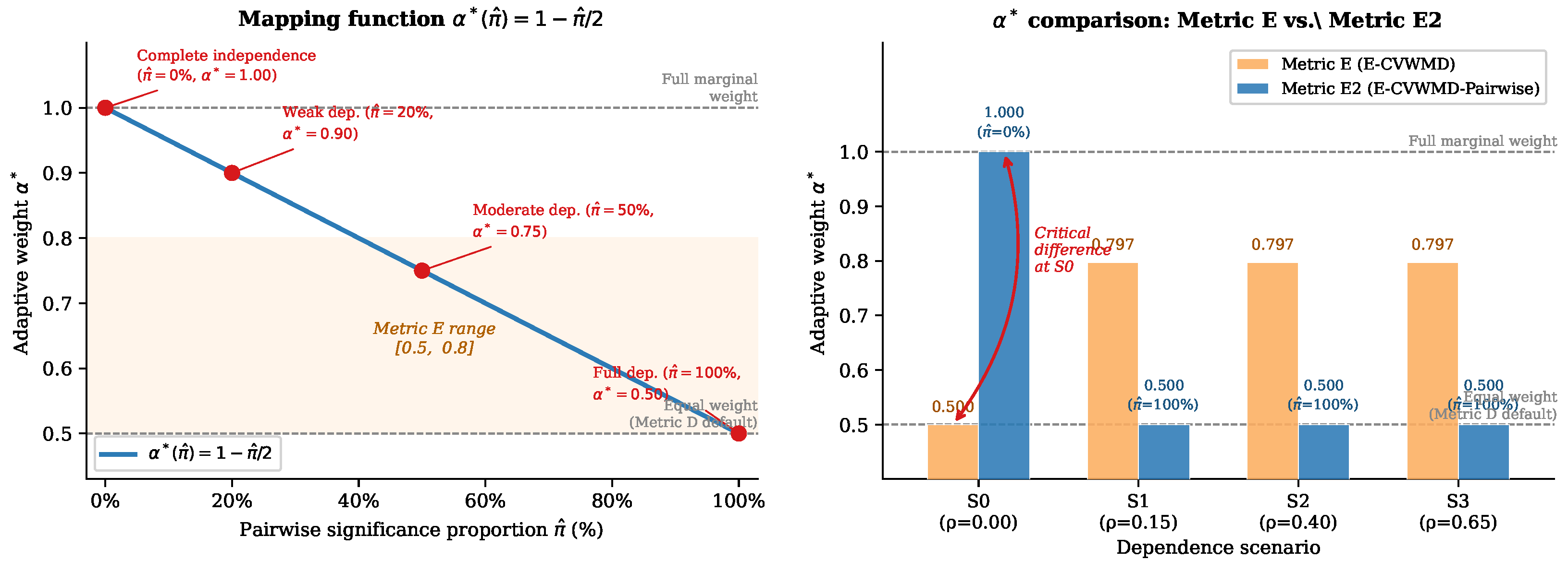
Justification of the linear mapping ${\alpha }^{\ast }$($\widehat{\pi }$) = 1 −$\widehat{\pi }$/2. The choice of a linear mapping between the pairwise significance index $\widehat{\pi }$ and the adaptive weight ${\alpha }^{\ast }$ is motivated by three considerations. First, the boundary constraints are axiomatically natural: $\widehat{\pi }=0$ (no residual correlation) implies the dependence term $S_{\mathrm{dep}}^E$ measures pure noise and should receive zero weight (${\alpha }^{\ast }=1$); $\widehat{\pi }=1$ (all pairs significantly correlated) implies the dependence structure is as complex as possible, warranting equal weight between marginal and dependence components (${\alpha }^{\ast }=0.5$), consistent with the MDD default. Second, linearity is the parsimony-preserving interpolant between these two anchors: it introduces no additional tuning parameters and ensures that every marginal increase in the proportion of correlated pairs is penalised by an equal decrease in ${\alpha }^{\ast }$. Third, the simulation study provides empirical support: across 37,440 model evaluations, the linear mapping produces correct discrimination in 14 of 15 conditions and outperforms Metric E by 27–40 percentage points in CDR across all block-structure studies. A formal decision-theoretic derivation—identifying the loss function for which Equation (15) minimises expected regret—is desirable and is left as an open theoretical problem; we regard the simulation evidence as sufficient justification for a practical metric.

Degradation of E2 at $\mathit{\rho }=\mathbf{0.90}$ (Study S1). Table 7 shows that E2’s CDR falls to 37.6% under full uniform correlation ($\rho =0.90$), below the 50% chance level. This behaviour has a structural explanation: when $\widehat{\pi }=1$ (all pairs significant), ${\alpha }_{E2}^{\ast }=0.50$, so equal weight is assigned to $S_{\mathrm{marg}}^E$ and $S_{\mathrm{dep}}^E$. The $S_{\mathrm{dep}}^E$ term is a Frobenius-norm comparison of two Spearman correlation matrices; when $\rho =0.90$, M3’s draw residuals (generated from ${\Sigma }_{\mathrm{true}}$) are highly correlated, while its prediction errors are small and near-uncorrelatedthe mismatch between the two matrices is large. Conversely, M1’s independent draw residuals and noise-washed prediction errors are both approximately uncorrelatedthe mismatch is small. The net result: $S_{\mathrm{dep}}^E\left(\mathrm{M}3\right)\gg S_{\mathrm{dep}}^E\left(\mathrm{M}1\right)$, inverting the correct ranking (Supplementary Figure S1 illustrates this mechanism with a synthetic demonstration where $S_{\mathrm{dep}}^E\left(\mathrm{M}3\right)=15.96$ vs. $S_{\mathrm{dep}}^E\left(\mathrm{M}1\right)=0.09$ over 30 replicates). This is a known limitation of residual-based dependence scores that do not account for the scale-accuracy interaction. A potential remedyrescaling $S_{\mathrm{dep}}^E$ by the marginal noise level or using convex ${\alpha }^{\ast }$ mappings (Table 14) is left for future work. Crucially, this degradation occurs only in the extreme homogeneous setting ($\rho =0.90$ uniform); in all heterogeneous structures (block, multi-block, sparse) studied in S2, S2b, and S3, E2 maintains CDR $>60\%$.

Comparison with the Energy Score (Metric B). Table 7 shows that Metric B (Energy Score) achieves CDR $\ge 69.8\%$ across all four $\rho$ levels in Study S1, outperforming E2 at $\rho =0.65$ (70.1% vs. 52.0%) and $\rho =0.90$ (69.8% vs. 37.6%). This comparison deserves explicit acknowledgement. The Energy Score is strictly proper and genuinely detects dependence misspecification through the $\mathbb{E}[\parallel \mathbf{Y}-{\mathbf{Y}}^{\prime }\parallel ]$ term, which effectively embeds joint structure. Three considerations justify Metric E2 as a complementary tool rather than a substitute. First, the Energy Score does not handle mixed-type outcome spaces natively; its embedding of the binary component $Y^{\left(K\right)}$ via predictive probability is a pragmatic extensioneffective in practice but not formally derived within the Energy Score framework of Gneiting and Raftery [1]. Second, the Energy Score assigns equal implicit weight to all variables, exacerbating scale heterogeneity in the manner identified by Koochali et al. [11]; E2’s CV-derived weights address this directly. Third, in the M1/M3 discrimination task (where models differ in both noise level and dependence structure), E2 provides better-calibrated discrimination for heterogeneous structures (block, multi-block, sparse)achieving CDR advantages of 27–40 pp over Metric E and maintaining CDR $>60\%$ across Studies S2, S2b, and S3. For the M5/M3 scenario (identical noise, differing dependence only), the Energy Score is the superior tool, as Table 10 confirms that E2 also fails there for $\rho >0$. The practical recommendation is therefore to report both E2 and the Energy Score, using E2 as the primary metric for heterogeneous mixed-type systems and Metric B as a robustness check for high-correlation regimes and when dependence detection with fixed marginal quality is required.

Practical decision guide: E2 vs. Energy Score. To make this recommendation actionable, we summarise the preference rule explicitly. Prefer E2 when: (i) the response space is genuinely mixed-type (continuous and binary outcomes), since the Energy Score’s binary embedding is a pragmatic rather than formally derived extension; (ii) variable-scale heterogeneity is substantial (high dispersion in CV values across outcomes), since the Energy Score’s equal-variable weighting exacerbates scale artefacts; and (iii) competing models differ in both noise level and dependence structure (the M1/M3 regime, which is the typical applied comparison). Prefer the Energy Score (Metric B) when: (i) models share identical marginal quality but differ only in dependence structure (the M5/M3 regime); (ii) near-saturated uniform correlation ($\rho \ge 0.65$) is expected and the quadratic mapping variant of E2 is not selected; or (iii) strict properness is required, in which case the E2-LL variant is also a valid alternative provided calibrated binary predictive probabilities are available. These two metrics are complementary, not competing; reporting both provides a comprehensive evaluation.

Statistical power and confidence intervals for CDR. The CDR estimates in Table 7 and Table 8 are based on 30 replicates per cell. Using the normal approximation for a binomial proportion, the 95% confidence interval for a CDR of p over 30 replicates has half-width $\pm 1.96\sqrt{p(1-p)/30}\approx \pm 9$ pp at $p=0.5$. Differences between metrics of 5–8 pp should therefore be interpreted cautiously. The large advantages reported for E2 over E in Studies S2 and S2b (27–40 pp) substantially exceed this margin and are robust to this limitation; the finer comparisons between E2 and Metrics A, B, D are indicative rather than definitive. Increasing to 100 replicates per cell in a follow-up study would provide half-width $\pm 5$ pp.

Notation glossary. To ease readability,

Table 13. Notation summary for Metrics E and E2.

Symbol	Definition
K, $K_c$	Total and continuous response dimensions
$w_k$, $w_{\mathrm{bin}}$	CV-derived weights for continuous and binary outcomes
$S_{\mathrm{marg}}^E$	CV-weighted marginal score (Step 2)
$S_{\mathrm{dep}}^E$	Residual-correlation Frobenius-norm dependence score (Step 3)
${\alpha }^{\ast }$	Data-adaptive marginal weight $\in [0.5,1]$
$p_{\mathrm{mv}}$	p-value of global distance-correlation test (Metric E, Step 4)
$\widehat{\pi }$	Proportion of pairwise Spearman tests significant after Holm correction (Metric E2, Step 4). Note: $\widehat{\pi }$ denotes this screening index throughout; the mathematical constant $\pi \approx 3.14159$ does not appear in the paper.
$P_{\mathrm{total}}$	$\left({\displaystyle \genfrac{}{}{0pt}{}{K}{2}}\right)$: total number of variable pairs
CDR	Correct discrimination rate: $Pr({\Delta }_f>0)$ over replicates
$\overline{\Delta }$	Mean discrimination Delta: $\overline{S_f\left(\mathrm{M}1\right)}-\overline{S_f\left(\mathrm{M}3\right)}$

collects the principal symbols introduced in this paper.

Properness and the Log-Loss variant. With the default Accuracy penalty, Metrics E and E2 are not strictly proper: $(1-{\mathrm{Acc}}^{\left(K\right)})$ depends only on the hard threshold ${\widehat{y}}^{\left(K\right)}\ge 0.5$, so a forecaster issuing the true probability can be outscored by one issuing a miscalibrated sharp forecast [1]. We address this directly rather than defer it. The strictly proper Log-Loss variant (E-LL/E2-LL), which replaces the Accuracy penalty with −$\sum ylog\widehat{p}+(1-y)log(1-\widehat{p})$, is implemented in mvmetrics v0.2.0 and re-evaluated across all simulation studies. The discrimination ranking is essentially unchanged: the Log-Loss variant is identical to the Accuracy version in most conditions and differs by at most 10 pp in CDR (mean $1.3$ pp), only in the high-correlation regime ($\rho \ge 0.65$), confirming that the joint ordering is not an artefact of the non-proper binary term (its contribution is bounded by $w_{\mathrm{bin}}=1/(K_c+1)=0.20$). We recommend the Log-Loss variant whenever calibrated probabilistic binary predictions are available and the Accuracy variant as a lightweight default for point-prediction pipelines where full predictive probabilities may not be produced by the model under evaluation.

Non-Gaussian copulas: future work. Formal evaluation of E2 under non-Gaussian dependence structures (Clayton lower-tail, Gumbel upper-tail) requires exact copula simulation via the copula R package [15]; such an evaluation is deferred to future work. Practitioners working in extreme-precipitation regimes should verify E2’s performance via simulation before deployment.

Software. Despite these limitations, Metrics E and E2 fill a documented gap: no existing paper develops joint performance metrics specifically for mixed-type multivariate responses within a cross-validation framework. The practical recommendation emerging from the simulation study is to use E2 as the primary joint metric for hydroclimatic systems with heterogeneous dependence structures, supplemented by the Energy Score (Metric B) and MDD decomposition (Metric D) for a comprehensive evaluation. The mvmetrics R package [16] (https://darango2025.github.io/mvmetrics, version 0.2.0) provides a reference implementation of all five families and the E2 pairwise refinement, with automated ranking and bootstrap confidence intervals. Version 0.2.0 adds the strictly proper Log-Loss variant, alternative weighting schemes (uniform, inverse-variance, and an origin-invariant SD scheme), effect-size and p-value pairwise screening, configurable multiple-testing correction, and alternative ${\alpha }^{\ast }\left(\widehat{\pi }\right)$ mappings. The package includes unit tests for all metric families and the pairwise screening procedure, and a regression test verifying that the default configuration reproduces the simulation engine of this paper to machine precision. We emphasise that E2 is offered as a practical, empirically validated diagnostic for heterogeneous mixed-type systems, not as a replacement for strictly proper scores; its strengths and the regimes where alternatives are preferable are delimited in the Limitations below.

Limitations

We summarise the principal limitations of Metrics E and E2 in one place.

Not strictly proper by default. As discussed above, the default Accuracy penalty is not a strictly proper scoring rule. The strictly proper Log-Loss variant removes this limitation at the cost of requiring calibrated probabilistic binary predictions.

Degradation under near-saturated uniform dependence. E2’s CDR falls below the chance level only in the extreme homogeneous regime ($\rho =0.90$ uniform), where the residual-correlation Frobenius term interacts adversely with marginal accuracy; the strictly proper Energy Score (Metric B) is preferable there and we recommend reporting it alongside E2 as a robustness check. In all heterogeneous structures (block, multi-block, sparse) E2 maintains CDR $>60\%$.

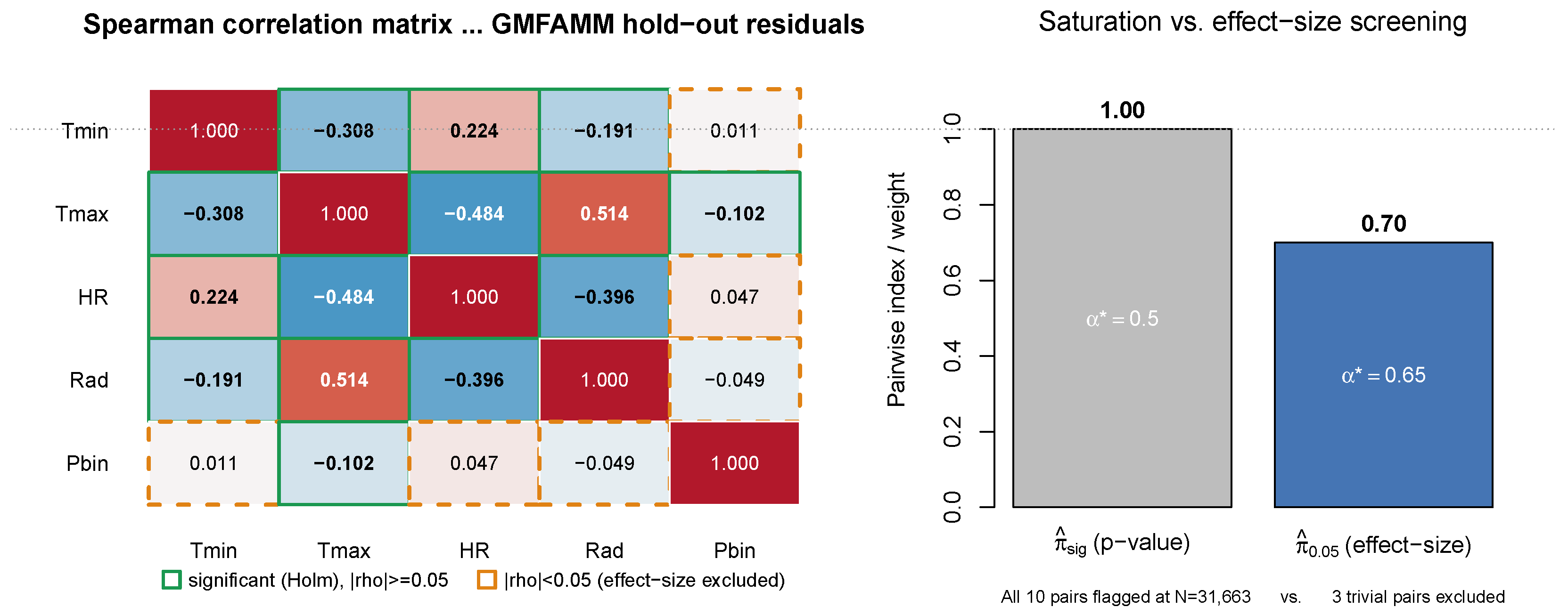
Sample-size sensitivity of $\widehat{\mathit{\pi }}$ and choice of ${\mathit{\rho }}_{\mathbf{0}}$. Because $\widehat{\pi }$ is built from significance tests, very large hold-out samples render negligible correlations “significant”: on the Valle del Cauca hold-out ($N\approx$ 31,663) all ten pairs are flagged, so the significance-based index saturates at ${\widehat{\pi }}_{\mathrm{sig}}=1.0$ (${\alpha }_{E2}^{\ast }=0.50$). The effect-size variant flags a pair as dependent only when $|{\widehat{\rho }}_s| \ge {\rho }_0$; raising ${\rho }_0$ from $0.05$ to $0.20$ moves $\widehat{\pi }$ from $0.70$ through $0.60$ (${\rho }_0=0.15$) to $0.50$ (${\rho }_0=0.20$), as detailed in Table 12. The choice of ${\rho }_0$ is N-dependent: for large samples ($N\gg {10}^3$) where significance saturates, ${\rho }_0\ge 0.05$ is recommended to exclude physically negligible correlations; for moderate samples ($N\sim 500$, as in the simulation), the significance-based threshold is more appropriate because residual correlations may be attenuated by model noise below common effect-size thresholdssensitivity analysis confirms that at $N=500$ and $\rho =0.40$, ${\rho }_0=0.05$ screening reduces E2 CDR from $100\%$ to $39\%$, while ${\rho }_0=0.15$ restores it to $100\%$. We recommend: use significance-based $\widehat{\pi }$ as default for small-to-moderate N; apply effect-size screening with ${\rho }_0\in [0.10,0.20]$ when $N>5000$; document the choice transparently.

Furthermore, the pairwise Spearman tests assume approximately exchangeable residuals. In settings with strong temporal autocorrelation or unmodelled spatial clusteringcommon in hydroclimatic station recordsthe effective sample size is smaller than $N_{\mathrm{test}}$, which inflates significance and can cause saturation even at moderate N. For such settings, a block-bootstrap correction or a more conservative effect-size threshold (${\rho }_0\ge 0.10$) is recommended before interpreting $\widehat{\pi }$.

Remark on the double-threshold issue. We acknowledge that the effect-size criterion ${\rho }_0$ substitutes one arbitrary threshold (the significance level ${\alpha }_{\mathrm{test}}$) for another (the correlation cutoff ${\rho }_0$). The practical advantage of ${\rho }_0$ over ${\alpha }_{\mathrm{test}}$ lies in its interpretabilitypairs with $|{\widehat{\rho }}_s| <{\rho }_0$ are operationally negligible for the application at handand in its resistance to saturation at large N, rather than in eliminating arbitrariness per se. The sensitivity of $\widehat{\pi }$ and ${\alpha }_{E2}^{\ast }$ to ${\rho }_0$ is fully documented in Table 12, and practitioners should report their chosen ${\rho }_0$ transparently.

Scale and origin dependence of CV weights. The coefficient of variation is scale-invariant but not origin-invariant: for variables on an interval scale (e.g., temperature in °C vs. K) the CV weight changes with the chosen zero. We therefore provide origin-invariant alternatives (SD-based and inverse-variance weighting); across all four schemes, the discrimination ranking is identical in every low- and moderate-correlation condition and changes by at most 13 pp (mean 2 pp), only at $\rho \ge 0.65$, indicating that the results are not an artefact of the CV choice. Recommendation: practitioners using interval-scale variables (temperature, pressure) should use the SD-based scheme as default; the CV scheme is most appropriate for strictly ratio-scale variables (precipitation, solar radiation) where the origin is physically meaningful. Both are implemented in mvmetrics v0.2.0.

Mapping and multiple-testing choices. The linear mapping ${\alpha }^{\ast }\left(\widehat{\pi }\right)=1-\widehat{\pi }/2$ (Figure 5) is one of several monotone interpolants satisfying the same qualitative boundary conditions. Alternative families include $1-\widehat{\pi }$, $1-{\widehat{\pi }}^{\gamma }$ for $\gamma >0$, or ${\displaystyle \frac{1}{1+c\widehat{\pi }}}$ for $c>0$; we study four concrete instances (linear, quadratic, cubic, square-root) that span the range from concave to convex curvature. The mapping choice is consequential in the saturated regime rather than innocuous.

Table 14. CDR (%) for Metric E2 under four ${\alpha }^{\ast }\left(\widehat{\pi }\right)$ mappings. Study S1, M1 vs. M3, averaged over $K\in \{3,5,10,15\}$, both distributions, both $p_{\mathrm{bin}}$, 30 replicates. Bold: highest CDR per row. The convex mappings (quadratic, cubic) recover CDR $=100\%$ even at $\rho =0.90$, providing a constructive remedy for E2’s high-$\rho$ degradation under the linear default.

$\mathit{\rho }$	Linear	Quadratic	Cubic	Square-Root
0.00	100.0	100.0	100.0	100.0
0.40	100.0	100.0	100.0	87.5
0.65	76.7	100.0	100.0	49.2
0.90	50.0	100.0	100.0	25.8

quantifies the impact: at $\rho =0.65$, the linear mapping gives CDR $=76.7\%$, while quadratic and cubic both recover CDR $=100\%$; at $\rho =0.90$, linear gives $50\%$ (chance level), while quadratic/cubic again give $100\%$, and square-root collapses to $25.8\%$. In all low- and moderate-correlation conditions ($\rho \le 0.40$), every mapping gives identical CDR $\ge 87.5\%$. This identifies a constructive remedy for the high-$\rho$ degradation: a convex mapping (quadratic or cubic) eliminates it at no cost in heterogeneous structures. The multiple-testing choice behaves similarly: Holm and Bonferroni yield the highest CDR, while omitting correction (none) inflates $\widehat{\pi }$ and degrades CDR by up to 100 pp in borderline high-correlation cells; the conservative Holm default is therefore preferred. We expose all four mappings and corrections as options and report this sensitivity rather than present any single choice as definitive. Although convex mappings (quadratic, cubic) eliminate the high-$\rho$ degradation of E2 at no cost in heterogeneous structures, we retain linear as the default for three reasons: (i) interpretive transparencyeach 10 pp increase in $\widehat{\pi }$ reduces ${\alpha }^{\ast }$ by exactly 5 pp, a one-to-one correspondence with no free curvature parameter; (ii) parsimonylinearity is the unique monotone interpolant between the two boundary anchors that introduces no additional hyperparameters; and (iii) backward compatibility with the simulation results reported in this paper. Users who anticipate near-saturated uniform dependence ($\rho \ge 0.65$) should set mapping = “quadratic” in mvmetrics::e2_score(), as Table 14 demonstrates that this eliminates the degradation entirely.

Table 15. CDR (%) for Metric E2 under four weighting schemes. Study S1, M1 vs. M3. CV: coefficient-of-variation weights (default); Uniform: equal weights; SD: standard-deviation weights (origin-invariant); InvVar: inverse-variance weights. Bold: highest CDR per row.

$\mathit{\rho }$	CV	Uniform	SD	InvVar
0.00	100.0	100.0	100.0	100.0
0.40	100.0	100.0	100.0	100.0
0.65	80.0	79.2	73.3	77.5
0.90	49.2	48.3	50.0	48.3

Maximum CDR difference across schemes: 6.7 pp at $\rho =0.65$; 1.7 pp at $\rho =0.90$. The discrimination ranking is identical across all schemes at $\rho \le 0.40$.

,

Table 16. CDR (%) for Metric E2 under four multiple-testing corrections. Study S1, M1 vs. M3. Holm: Holm–Bonferroni (default); BH: Benjamini–Hochberg; Bonf: Bonferroni; None: uncorrected p-values. Bold: highest CDR per row.

$\mathit{\rho }$	Holm	BH	Bonf	None
0.00	100.0	100.0	100.0	100.0
0.40	100.0	100.0	100.0	65.8
0.65	76.7	70.0	79.2 †	47.5
0.90	48.3	47.5	50.0	37.5

^† Bonferroni is slightly more conservative than Holm at $\rho =0.65$, recovering a marginally higher CDR through a lower false-positive rate. Omitting correction (None) inflates $\widehat{\pi }$, degrades CDR by up to 34 pp at $\rho =0.40$ and worsens discrimination uniformly. Holm and Bonferroni give the best and most consistent performance; Holm is preferred for its sequentially rejective efficiency.

and

Table 17. CDR (%) for Metrics E and E2 under Accuracy (default) and Log-Loss binary scoring. Study S1, M1 vs. M3. Max CDR difference between variants: 3.3 pp for E2 (at $\rho =0.65$); 3.4 pp for E (at $\rho =0$). Bold: highest CDR per row within each metric.

	Metric E		Metric E2
$\mathit{\rho }$	Accuracy	Log-Loss	Accuracy	Log-Loss
0.00	100.0	100.0	100.0	100.0
0.40	4.2	0.8	100.0	100.0
0.65	0.0	0.0	78.3	76.7
0.90	0.0	0.0	50.0	48.3

The Log-Loss variant leaves the joint discrimination ordering essentially unchanged: differences are ≤3 pp in CDR (mean 1.3 pp), confirming that the binary term ($w_{\mathrm{bin}}=0.20$) is not the driver of the reported performance. We recommend the Log-Loss variant whenever calibrated probabilistic binary predictions are available.

provide the quantitative evidence backing the three text claims in this Limitations section. All tables use Study S1, M1 vs. M3, averaged over $K\in \{3,5,10,15\}$, both distributions, both $p_{\mathrm{bin}}$, 30 replicates.

Single application system. The real-data evaluation uses one hydroclimatic system (Valle del Cauca); the CV weights and $\widehat{\pi }$ are system-specific and require recalibration elsewhere, although the methodology is system-agnostic. The practical recalibration protocol is: (i) compute CV (or SD, for interval-scale variables) weights on the training partition of the target system; (ii) run pairwise Spearman tests on hold-out residuals with Holm–Bonferroni correction; (iii) for large hold-out samples ($N\gg {10}^3$), apply effect-size screening with ${\rho }_0\in [0.05,0.20]$ to prevent saturation; and (iv) compute ${\alpha }^{\ast }\left(\widehat{\pi }\right)$ with the linear mapping (or a convex alternative if high uniform correlation is suspected). This four-step protocol is fully automated in mvmetrics v0.2.0.