Extreme Rainfall Modelling Using Time-Varying Threshold Generalised Pareto Regression Trees

Abstract

The escalating frequency and intensity of extreme rainfall events driven by climate change threaten infrastructure resilience and societal safety, underscoring the urgent need for robust models to predict these events. Previous studies on the integration of Extreme Value Theory (EVT) and machine learning in modelling extreme rainfall events have not explored the use of a time-varying threshold. This study introduces a novel time-varying threshold Generalised Pareto (GP) regression tree for modelling extreme rainfall in Durban, South Africa. The proposed hybrid model combines EVT with covariate-driven regression tree partitioning, allowing the threshold to evolve dynamically with meteorological conditions. Using daily rainfall and meteorological covariate data from 1981 to 2025, the model was developed, pruned, and benchmarked against a static-threshold GP regression tree and a time-varying threshold Generalised Pareto Distribution (GPD). Evaluation based on the Bayesian Information Criterion (BIC) and log-likelihood demonstrated the superior performance of the proposed model in capturing covariate-driven heterogeneity and temporal variability of rainfall extremes. Four distinct climatic regimes with different tail behaviours and return levels were identified. This study provides the first meteorological application of a time-varying threshold GP regression tree and offers practical insights into flood risk assessment and climate resilience planning in the city of Durban.

1. Introduction

The stability of human societies, the integrity of infrastructure, and the health of global ecosystems are increasingly threatened by the escalating frequency and intensity of extreme rainfall events [1]. Driven by a changing climate, these phenomena precipitate disasters such as catastrophic flooding and landslides, posing a formidable challenge to the resilience of modern agriculture and the efficacy of urban planning and disaster management [2,3]. Within this high-stakes context, the ability to accurately forecast extreme events is a critical requirement for the development of effective adaptation and mitigation strategies aimed at minimising the risks and consequences associated with climate-related disasters.

South Africa has experienced numerous catastrophic rainfall events over the past five decades, resulting in significant loss of life and widespread damage [4]. Notable examples include the 1981 Laingsburg flood, which claimed more than 100 lives [5], and the September 1987 KwaZulu-Natal (KZN) floods, the deadliest in the country’s history, with over 500 fatalities [6]. The country has also been affected by tropical cyclones such as Domoina (1984), Eline (2000), and Eloise (2021), as well as the unprecedented April 2022 Durban floods, which killed 443 people and displaced thousands [7,8]. These events, often characterised by rainfall totals reaching 400 mm within 24 h and driven by cut-off lows, tropical cyclones, or tropical–temperate interactions [9], highlight the urgent need for models capable of capturing the tail behaviour of rainfall distributions. This need is reinforced by climate projections from Pinto et al. [7], which indicate that extreme rainfall events are likely to increase in frequency and severity, amplifying their societal impacts.

1.1. Rationale

This study tackles the issue of accurate modelling of extreme rainfall to enhance disaster preparedness and mitigation efforts. The intensification of extreme rainfall events due to climate change has led to profound socio-economic and environmental consequences, yet their unpredictable nature makes accurate modelling extremely challenging [10]. Failure to develop a deeper understanding of these patterns and the ability to accurately predict them can lead to severe socio-economic consequences, including significant loss of life and extensive damage to critical infrastructure [11]. For instance, the heavy rainfall, flooding, and landslides in the southeast region of South Africa resulted in approximately 448 deaths, displaced over 40,000 individuals, and destroyed more than 12,000 shelters [6]. These catastrophic events highlight the urgent need for advanced modelling techniques specifically tailored to local contexts.

Traditional models, such as the Generalised Pareto Distribution (GPD), while statistically rigorous, often rely on assumptions of data homogeneity and struggle to account for complex, covariate-driven variability and the non-stationary nature of rainfall extremes in dynamic atmospheric systems. More recently, machine learning techniques have obtained traction in predicting rainfall due to their capacity to capture intricate, non-linear relationships within climate data [12,13]. Although hybrid model which combine statistical and machine learning methods have shown some promise in enhancing the reliability of extreme rainfall predictions, the direct integration of the GPD into tree-based models for extreme value modelling remains largely underexplored, with the Generalised Pareto (GP) regression tree approach previously being limited to domains such as cyber claim analysis. This study introduces a novel extension of the GP regression tree that incorporates a time-varying threshold, allowing the model to adapt to non-stationary climate behaviour. It applies this advanced method for the first time to model extreme rainfall. It is important to note that the covariates employed in this study are meteorological in nature (daily humidity, pressure, temperature, and wind variables) and are therefore suited to capturing regime-based heterogeneity in daily rainfall extremes rather than long-term climate change trends. The primary contribution of this work is methodological: demonstrating how a time-varying threshold GP regression tree can improve upon classical stationary frameworks by conditioning on atmospheric state, a capability that is equally relevant to both short-range weather extremes and, with appropriate substitution of slowly varying climatological predictors, to climate change applications.

1.2. Review of the Literature

Modelling extreme rainfall remains a complex challenge in hydrometeorology due to the non-linear and non-stationary nature of rainfall-generating processes. Traditional statistical approaches grounded in Extreme Value Theory (EVT) have long provided a foundation for modelling the tails of rainfall distributions, offering valuable insights into the frequency and magnitude of rare events. Within EVT, the Peaks-over-Threshold (POT) approach using the GPD and the block-maxima approach using the Generalised Extreme Value Distribution (GEVD) are the most common tools [14,15]. These models have been widely applied to characterise heavy rainfall in diverse regions, demonstrating their robustness for estimating return levels and understanding extreme rainfall behaviour.

The GPD, in particular, has proven effective at representing exceedances over high thresholds and has been applied extensively globally. Studies such as those by Phoophiwfa et al. [16], Singirankabo and Iyamuremye [17], and Sunday et al. [18] have successfully employed the GPD to estimate return levels and assess rainfall intensities over various temporal scales. However, the effectiveness of these models is often constrained by their dependence on a fixed threshold and the assumption of stationarity, which limits their ability to capture changing climatic dynamics. Research in South Africa and elsewhere reveals increasing evidence of non-stationarity in rainfall extremes, where the statistical properties of extreme events evolve over time [19,20]. For example, McBride et al. [19] observed a significant rise in the frequency of extreme daily rainfall events across multiple South African regions during the latter half of the twentieth century, while Sikhwari et al. [20] found that EVT models, although informative, often fail to capture spatial variability and evolving climate drivers.

To address the limitations of classical EVT, researchers have explored non-stationary extensions in which model parameters or thresholds vary as functions of covariates such as temperature, surface pressure, or time [21,22,23]. These models aim to account for changes in climatic forcing and anthropogenic influence, enabling a more flexible representation of extreme rainfall trends. For instance, Tugrul et al. [22] projected substantial increases in extreme rainfall return levels in Turkey under different climate scenarios, while Musayidizi [21] demonstrated the benefits of incorporating temperature and population as covariates in GPD modelling. Nevertheless, such approaches remain largely parametric and struggle to capture the complex, high-dimensional dependencies inherent in atmospheric systems. Their reliance on linear or smoothly varying relationships limits their performance in settings characterised by abrupt transitions, localised variability, or non-linear interactions between multiple meteorological drivers.

The emergence of machine learning and deep learning techniques has provided new avenues for modelling rainfall by learning complex and non-linear relationships from large datasets without strict parametric assumptions. Deep learning architectures, including Convolutional Neural Networks (CNNs), Recurrent Neural Networks (RNNs), and Long Short-Term Memory (LSTM) networks, have demonstrated strong capabilities in capturing temporal dependencies and spatial features of rainfall data [12,24]. Studies have shown that these models outperform traditional statistical regressors in predicting rainfall, particularly in data-rich contexts where long-term climate interactions can be learnt directly from input variables [25,26,27]. CNNs have proven particularly effective in recognising spatial rainfall patterns and forecasting flood-inducing events, while bidirectional LSTM architectures excel in learning sequential dependencies in rainfall time series, making them suitable for multi-day rainfall prediction [24,27].

Beyond deep learning, tree-based ensemble methods such as Random Forests (RFs) and Extreme Gradient Boosting (XGBoost) have shown remarkable predictive strength for rainfall classification and forecasting tasks [28,29]. RFs, in particular, are popular due to their interpretability, robustness to noise, and ability to capture non-linear relationships across predictors. Ogunniyi et al. [29] applied RF models to forecast monthly rainfall across South Africa’s climatic zones and found strong alignment between model predictions and observed rainfall patterns, demonstrating their operational potential in data-scarce environments. Despite these successes, purely data-driven models are often limited in their ability to extrapolate beyond the observed data range, which is critical when predicting extremes. Moreover, they generally lack theoretical grounding in the statistical properties of rare events and can exhibit biases in the presence of class imbalance, where extreme rainfall occurrences represent only a small fraction of total observations.

Recognising these limitations, recent studies have sought to combine the strengths of EVT and machine learning, resulting in hybrid frameworks that integrate statistical tail modelling with machine learning algorithms. These approaches maintain the interpretability and theoretical soundness of EVT while leveraging the predictive flexibility of machine learning to capture complex covariate interactions. Anco-Valdivia et al. [30] used RF regression to estimate rainfall return levels in semi-arid Peru, achieving improved accuracy over conventional GPD fits by allowing data-driven mapping between rainfall intensity and covariates. Velthoen et al. [31] proposed the Gradient Boosting Extreme Value (GBEX) algorithm, which embeds GPD deviance into a boosting framework, enabling the estimation of covariate-dependent tail parameters. Their results showed that GBEX outperformed standard quantile regression and POT-based approaches in predicting high quantiles of precipitation. Similarly, Gnecco et al. [32] introduced the Extremal Random Forest (ERF), a method that estimates conditional GPD parameters through local likelihood estimation, enabling flexible, data-driven tail inference. In another advancement, Grazzini et al. [33] developed the MaLCoX model, which uses RF classifiers to post-process numerical weather forecasts for identifying extreme precipitation events, achieving greater predictive skill and longer lead-time reliability than deterministic forecasts.

Among the most theoretically appealing yet under-explored hybrid methods is the GP regression-tree model introduced by Farkas et al. [34,35,36]. The technique merges recursive partitioning with EVT by fitting GPDs at each split point to select the covariate and split point that minimise the GPD negative log-likelihood of GPD. Consequently, fitting GPDs to threshold exceedances within each terminal node of a regression tree, allowing the scale and shape parameters to vary across covariate-defined subregions. This yields interpretable, localised tail models that reflect heterogeneity in driving factors. Theoretical developments by Farkas et al. [36] confirmed the model’s statistical consistency and its ability to reduce misspecification bias relative to global EVT fits. To date, the GP regression trees approach has been primarily developed and applied by Farkas et al. [35,36], who have focused on cyber claim analysis and simulated predictions of flood event costs in France. Beyond their work, the method has received little to no attention in other domains, particularly in modelling extreme rainfall.

The proposed time-varying threshold GP regression tree differs fundamentally from existing non-stationary POT and EVT-boosting approaches. Non-stationary POT models allow the threshold, scale, and shape parameters to vary as functions of covariates, typically assuming that these changes can be modelled via smooth parametric or semi-parametric functions to capture the evolving and heterogeneous nature of extreme events [14]. In contrast, the proposed model adopts a regime-based framework in which covariate-driven heterogeneity is captured through likelihood-based recursive partitioning, enabling abrupt transitions between meteorological regimes. EVT-boosting methods embed GPD likelihoods within global additive models but do not explicitly identify locally homogeneous tail regimes. By integrating a covariate-dependent threshold directly into the tree-building process and fitting local GPDs within terminal nodes, the proposed approach separates regime discovery from tail extrapolation and relies on local stationarity rather than global smoothness assumptions.

This study addresses the gap in the literature by extending the GP regression tree framework to forecast extreme rainfall using a time-varying threshold. This methodological advancement enables the model to account for temporal shifts in climate behaviour and improves its responsiveness to non-stationary extreme rainfall patterns. By combining the flexibility of tree-based learning for handling high-dimensional, non-linear relationships with the robustness of the GPD in modelling threshold exceedances, this study presents a more adaptive and context-conscious modelling tool. To the best of our knowledge, this is the first application of time-varying threshold GP regression trees in meteorology and specifically for modelling extreme rainfall in the South African context. The study not only fills a methodological gap but also contributes practically by enhancing early warning capabilities and informing decision-making on disaster risk management, climate resilience, and infrastructure planning.

1.3. Research Highlights and Contribution of the Study

A novel time-varying threshold GP regression tree model is introduced for modelling extreme rainfall in Durban, South Africa. It dynamically adjusts exceedance thresholds based on meteorological covariates, blending extreme value theory tail modelling with the adaptive regression tree method to capture non-stationary rainfall extremes. Evaluation against the static threshold GP regression tree model and time-varying threshold GPD shows that the time-varying threshold GP regression tree model significantly outperforms alternatives by modelling covariate-driven heterogeneity in extreme rainfall. The analysis also reveals distinct climatic regimes in Durban with unique extreme rainfall characteristics, offering actionable insights for flood risk assessment and climate resilience planning.

The study makes the following scientific and methodological contributions:

(a)

Extends the GP regression tree framework by integrating a dynamic, covariate-dependent threshold, enhancing its ability to model non-stationary extreme rainfall processes.

(b)

Presents the first known application of a time-varying threshold GP regression tree in meteorological modelling, specifically applied to extreme rainfall in Durban, South Africa.

(c)

Effectively captures covariate-driven heterogeneity in extreme rainfall events by allowing both the threshold and GP parameters to vary with meteorological conditions, thereby identifying non-stationary behaviours often overlooked by static approaches.

(d)

Identifies four distinct climatic regimes, each characterised by unique GP parameters and return levels, enabling more localised and temporally adaptive estimation of rare rainfall extremes.

(e)

Benchmarks the proposed model against a fixed-threshold GP regression tree and a time-varying threshold GP distribution, consistently achieving superior performance as measured by the BIC and log-likelihood.

(f)

Improves return-level estimation by fitting GP models within homogeneous data segments, resulting in more precise quantification of rare rainfall magnitudes and frequencies for early-warning systems.

(g)

Provides practical implications for flood risk mitigation, infrastructure planning, and climate resilience, demonstrating the model’s value as a decision-support tool in climate-vulnerable regions.

The rest of the paper is organised as follows: Section 2 presents the models. Empirical results are discussed in Section 3. A detailed discussion of the results is presented in Section 4 and Section 5 concludes the paper.

2. Materials and Methods

This section presents the methodological framework for developing a time-varying threshold GP regression tree model designed to forecast extreme rainfall events. It briefly describes the study area and data sources, including long-term rainfall observations and key meteorological covariates. The methodological design integrates the principles of EVT within a regression tree structure to model the tail behaviour of rainfall distributions. Model optimisation is achieved through pruning to enhance parsimony, while performance is evaluated using established statistical criteria and validation procedures to ensure modelling accuracy and reliability.

During the preparation of this published version of the manuscript, the authors used generative artificial intelligence solely for language editing, sentence rephrasing, and improving clarity or conciseness in some parts of the text. All scientific content, including study design, data collection and processing, statistical modelling, analyses, interpretation of results, and the creation of figures and tables, was carried out entirely by the authors. The authors reviewed and edited all AI-assisted output and take full responsibility for the content of this publication.

2.1. Data Source and Area of Study

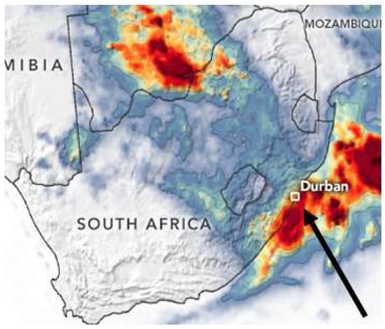
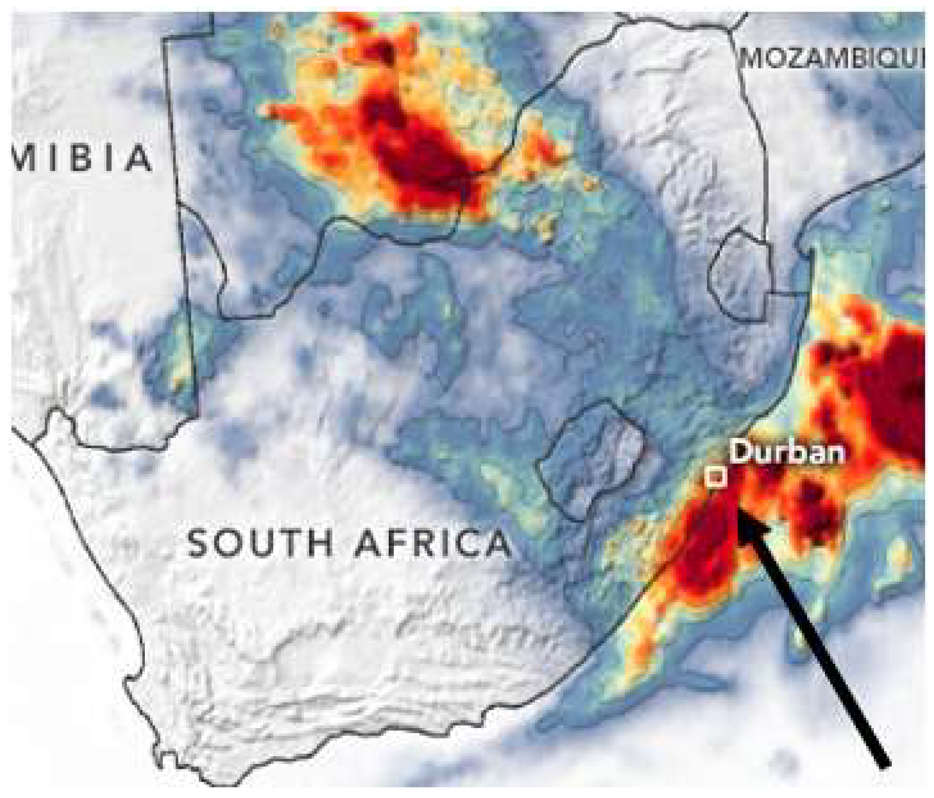
The study area is Durban, a seaside city in the KZN province of South Africa, which has been prone to extreme weather events and disastrous floods in recent decades [6,37]. Situated along the southeastern coast, Durban features diverse topography, including coastal plains and hilly terrain, which presents a valuable test case for evaluating the performance of the time-varying threshold GP regression tree model. This region was selected due to its high variability in precipitation patterns, socio-economic vulnerability to climate extremes, and the availability of long-term meteorological data from multiple observation stations. Durban has recorded several high-impact rainfall episodes in recent decades, making the region particularly suitable for modelling rare and severe weather events. Figure 1 presents the study area.

This study utilises secondary daily rainfall data from the National Aeronautics and Space Administration (NASA) Power Project, publicly accessible at https://power.larc.nasa.gov/data-access-viewer/ (accessed on 25 May 2026). The dataset spans from 1 January 1981 to 30 June 2025 and comprises key meteorological predictor variables, including surface pressure, relative humidity, wind speed, and temperature, with rainfall designated as the primary response variable. For model development and validation, the dataset is divided into training and testing subsets using an 80:20 chronological split. A chronological rather than random split is adopted to reflect the temporal structure of the rainfall series and ensure that model evaluation simulates genuine modelling of future extreme events. This approach provides a fair assessment of generalisability and helps to avoid overfitting. The training set contains 10,537 daily observations from 1 February 1981 to 3 January 2017, while the testing set comprises 2635 daily observations from 4 January 2017 to 30 June 2025. The training subset was used to fit the time-varying threshold GP regression tree model. In contrast, the testing subset was reserved exclusively for evaluating the predictive performance of the model on unseen data. It is noted that the test period includes the catastrophic April 2022 Durban flood event, one of the most extreme rainfall episodes recorded in the region. The inclusion of this event provides a stringent out-of-sample test of the model’s capacity to represent extreme tail behaviour. While this may favour models with heavier or more flexible tails, it also reflects the practical requirement that extreme-event models remain valid during the very episodes for which they are intended.

2.2. Regression Trees

Regression trees handle nonlinear heterogeneity by identifying clusters within the data. Let Y represent the response variable, specifically daily rainfall and $\mathbf{X}\in {\mathbb{R}}^t$ denote a vector of covariates. We observe an independent and identically distributed sample ${\left\{(Y_i,{\mathbf{X}}_i)\right\}}_{i=1}^n$ of realisations of $(Y,\mathbf{X})$. The primary goal of regression trees is to define decision rules that classify observations into rainfall categories based on their characteristics ${\mathbf{X}}_i$. These models are especially suitable when the diversity in covariate profiles leads to heterogeneous behaviour. The effectiveness of the tree depends on the intended focus, whether targeting the central tendency or the tail of the distribution, which in turn determines the choice of an appropriate loss function for evaluating the splits during the clustering phase. As modelling tools, regression trees introduce structure by partitioning observations into subsets, within which different regression models are applied. The aim is to estimate a regression function $m^{*}$ that minimises the expected loss,

$$m^{*}=arg\underset{m\in \mathcal{M}}{min}\mathbb{E}\left[\varphi (Y,m(\mathbf{X}\left)\right)\right],$$

where $\varphi$ is a chosen loss function and $\mathcal{M}$ denotes a class of candidate models. In this study, the negative log-likelihood is adopted as the loss function given by

$$\varphi (y,m\left(\mathbf{x}\right))=-log{f}_{m\left(\mathbf{x}\right)}\left(y\right),$$

(1)

which assumes a conditional distribution $Y|\mathbf{X}=\mathbf{x}$ belonging to a parametric family $\mathcal{F}$.

The data is split iteratively by identifying, at each step, a rule based on a covariate to divide the data into two more uniform groups. This process consists of two main stages, namely, the growing phase, which employs the Classification and Regression Trees (CART) algorithm to build the tree, and the pruning phase, where a subtree is extracted from the initial structure. The pruning stage serves as a model selection method.

2.2.1. Growing Phase

This phase is about building the initial and most detailed regression tree. It works by repeatedly finding the best ways to divide the data into smaller, more similar groups. Recursively, it divides the data into two child nodes at each step, based on the rules for a selected covariate. To split the data, the algorithm determines a set of rules

$$\mathbf{x}=(x^{\left(1\right)},\cdots ,x^{\left(t\right)})\to T_q\left(\mathbf{x}\right)$$

(2)

at each node, where $x^{\left(1\right)}$ represents a rule corresponding to the first independent variable and $x^{\left(t\right)}$ for the t-th independent variable. For each possible covariate x, $T_q\left(\mathbf{x}\right)=1$ or 0 depending on whether some conditions are satisfied, with $T_q\left(\mathbf{x}\right)T_{q^{\prime }}\left(\mathbf{x}\right)=0$ for $q\ne q^{\prime }$ and ${\sum }_q{T}_q\left(\mathbf{x}\right)=1$. Since each node of the tree results into two child nodes, each $T_q$ in Equation (2) generates two rules $T_{q1}$ and $T_{q2}$, for node 1 and node 2, respectively. Below is a step-by-step of how the algorithm works.

• Initialisation: The algorithm starts with all the data in one big group, with a single $T_1\left(x\right)=1$ representing the initial group rule that applies to all data points $\mathbf{x}$ at the very first step of the algorithm. Let $n_1=1$, represent one group at the initial step.
• Recursive rule splitting: At each step $k+1$, the existing rules $(T_1,\cdots ,T_{\left(n_k\right)})$ are considered. For each rule $T_q$:

  (a)

  If all observations satisfying $T_q\left({\mathbf{X}}_i\right)=1$ share identical characteristics, the rule remains unchanged.

  (b)

  Otherwise, $T_q$ is split into two new rules $T_{q1}$ and $T_{q2}$ based on an optimal threshold $x_{*}^{\left(a\right)}$. The threshold minimises the splitting criterion

  $$\begin{array}{cc}\hfill \mathsf{\Phi }\left(T_q,x^{\left(a\right)}\right)=& {\displaystyle \sum _{i=1}^n}\varphi (Y_i,m_{a-}({\mathbf{X}}_i,T_q))1_{X_i^{\left(a\right)}\le x^{\left(a\right)}}{T}_q\left(\mathbf{x}\right)\hfill \\ \hfill +& {\displaystyle \sum _{i=1}^n}\varphi (Y_i,m_{a+}({\mathbf{X}}_i,T_q))1_{X_i^{\left(a\right)}>x^{\left(a\right)}}{T}_q\left(\mathbf{x}\right),\hfill \end{array}$$

  (3)

  where

  $$\begin{array}{cc}\hfill m_{a-}(x,T_q)=& arg\underset{m\in \mathcal{M}}{min}{\displaystyle \sum _{i=1}^n}\varphi (Y_i,m\left({\mathbf{X}}_i\right))1_{X_i^{\left(a\right)}\le x}{T}_q\left({\mathbf{X}}_i\right),\hfill \\ \hfill m_{a+}(x,T_q)=& arg\underset{m\in \mathcal{M}}{min}{\displaystyle \sum _{i=1}^n}\varphi (Y_i,m\left({\mathbf{X}}_i\right))1_{X_i^{\left(a\right)}>x}{T}_q\left({\mathbf{X}}_i\right).\hfill \end{array}$$

  The best splitting variable a and the threshold $x_{*}^a$ selected as:

  $$\begin{array}{c}\hfill \hat{a}=arg\underset{a}{min}\mathsf{\Phi }(T_q,x_{*}^{\left(a\right)}).\end{array}$$

  The new rules are defined as follows:

  • $T_{q1}\left(\mathbf{x}\right)=T_q\left(\mathbf{x}\right)1_{X_i^{\left(\hat{a}\right)}\le x_{*}^{\left(\hat{a}\right)}},$
  • $T_{q2}\left(\mathbf{x}\right)=T_q\left(\mathbf{x}\right)1_{X_i^{\left(\hat{a}\right)}>x_{*}^{\left(\hat{a}\right)}}.$

• Stopping criteria: The growth continues until $n_{(k+1)}$ equals $n_k$, indicating that no further splitting is possible, where $n_{(k+1)}$ denote the new number of current groups and $n_{\left(k\right)}$ representing the number of groups in the previous step.

The binary tree structure grows as each rule $T_q$ generates two new child rules, forming new leaves at each step. The leaves represent the segmentation of the dataset.

2.2.2. Pruning Phase

The pruning phase is a crucial step that follows the initial growing phase in building a regression tree. While the growing phase creates a very detailed tree often called the maximal tree, this maximal tree can sometimes be overly complex and fit the training data too perfectly, leading to poor performance on new, unseen data. The pruning phase aims to find a simpler, more generalised tree from this maximal tree, striking a balance between simplicity and good predictive accuracy. In this study, the penalty parameter A in Equation (4) was selected via 10-fold cross-validation on the training dataset, evaluating the penalised GPD deviance across a grid of candidate values. The value minimising the cross-validated criterion was retained. This cross-validation step is separate from, and precedes, the final model evaluation. A subtree G of the maximal tree consists of a subset of rules, $T^G=\{T_1^G,\cdots ,T_{n_G}^G\}$, where $n_G$ is the number of leaves or terminal nodes. The pruning algorithm aims to minimise a penalised criterion:

$$C_A\left(G\right)={\displaystyle \sum _{i=1}^n}\varphi \left(Y_i,m^{T^G}\left({\mathbf{X}}_i\right)\right)+A·n_G,$$

(4)

where $\varphi \left(Y,m\left(\mathbf{X}\right)\right)$ is the loss function, $m^{T^G}$ is the estimated function for a specific subtree G, A represents a penalisation constant controlling the trade-off between fit quality and tree complexity, and n is the total number of data points.

Among all possible subtrees, the algorithm identifies the one with the smallest $C_A\left(G\right)$ in Equation (4). This process ensures that simpler trees with fewer leaves are penalised less, promoting parsimony. Instead of enumerating all subtrees, the algorithm considers only critical subtrees $G_J$ for $J=0,1,\cdots$, where $G_J$ minimises $C_A\left(G\right)$ for a fixed number of leaves $n_G=J$. The critical subtrees are determined iteratively since $G_{J+1}$ is obtained by removing one leaf from $G_J$. The penalty constant A is selected using a testing set or k-fold cross-validation. For a testing set, the data is split into a training set for tree construction and a test set for evaluating pruning performance. For k-fold cross-validation, the dataset is split into k parts, each alternately used for training and testing. Once A is optimised, the final tree $G^{*}\left(A\right)$ is chosen, and the corresponding regression function is $\hat{m}\left(\mathbf{x}\right)=m^{\hat{G}\left(\hat{A}\right)}\left(\mathbf{x}\right)$. In practice, critical subtrees are identified using an iterative backward elimination process starting from the maximal tree.

2.3. Time-Varying Threshold Generalised Pareto Distribution

The time-varying threshold Generalised Pareto Distribution (GPD) extends the classical Peaks-over-Threshold (POT) framework to accommodate non-stationary extreme behaviour by allowing the threshold and tail parameters to depend on time and meteorological covariates. Let $u\left(t\right)$ denote a covariate-dependent threshold, allowing the exceedance level to adapt to changes in atmospheric or temporal conditions. Let $Z_i=Yi-u\left(t\right)$, for $Y_i>u\left(t\right)$ denote exceedances. The distribution of $Z_i$ is assumed to follow a GPD with scale parameter $\sigma \left(\mathbf{x}\right)>0$ and shape parameter $\xi \left(\mathbf{x}\right)$, such that

$$\begin{array}{ccc}\hfill Pr(Z_i\le z\mid Y_i>u\left(t\right))& =& \left\{\begin{array}{cc}1-{\left(1+{\displaystyle \frac{\xi \left(\mathbf{x}\right)z}{\sigma \left(\mathbf{x}\right)}}\right)}^{-1/\xi \left(\mathbf{x}\right)},\hfill & \xi \left(\mathbf{x}\right)\ne 0,\hfill \\ 1-exp\left(-{\displaystyle \frac{z}{\sigma \left(\mathbf{x}\right)}}\right),\hfill & \xi \left(\mathbf{x}\right)=0,\hfill \end{array}\right.\hfill \end{array}$$

(5)

where $\xi \left(\mathbf{x}\right)$ and $\sigma \left(\mathbf{x}\right)$ are the covariate-dependent shape and scale parameters, respectively. Allowing the threshold to vary with time or covariates does not invalidate the POT approximation, provided that the threshold $u\left(t\right)$ is sufficiently high to ensure that exceedances lie in the tail of the underlying distribution, satisfying the principle of threshold stability. Within locally homogeneous covariate regimes, the exceedances must display tail equivalence, meaning that they share the same limiting GPD, with only smooth variations in scale and shape parameters. The asymptotic justification for the GPD remains valid under gradual temporal or covariate-driven changes, as established in non-stationary EVT [14,38]. In practice, these conditions are approximated by selecting a covariate-dependent threshold from the conditional distribution of rainfall, which ensures a sufficient number of exceedances for reliable inference while remaining high enough to meet POT assumptions. This framework allows the time-varying threshold GPD model to flexibly capture non-stationary extremes while maintaining a sound theoretical basis.

Due to the threshold stability property of the GPD, the scale parameter is not invariant to the choice of threshold. Specifically, if the threshold is increased, the corresponding scale parameter adjusts accordingly. In the present formulation, where the threshold $u\left(t\right)$ varies with covariates, the scale parameter $\sigma \left(\mathbf{x}\right)$ should therefore be interpreted as the conditional scale associated with the chosen covariate-dependent threshold. This ensures consistency with the theoretical foundations of extreme value theory under non-stationarity.

This time dependence in the threshold, coupled with the covariate dependence of the shape and scale parameters, enables modelling non-stationary tail behaviours where the definition of an extreme event and its distributional characteristics change over time or with other relevant factors. By allowing for a dynamic threshold and covariate-dependent shape and scale parameters, this extension of the GPD offers a flexible way to analyse and forecast extreme events when their occurrence level, tail shape, and tail scale are all subject to change.

2.4. Time-Varying Threshold Generalised Pareto Regression Trees

Time-varying threshold GP regression trees adapt regression trees to model the tail behaviour of a distribution. This is achieved by integrating the GPD likelihood directly into the tree-building process. Let z denote an exceedance above a time-varying threshold. The splitting criterion is based on the negative GPD log-likelihood, defined as the loss function

$$\varphi \left(z,m\left(\mathbf{x}\right)\right)=-log\sigma \left(\mathbf{x}\right)-\left({\displaystyle \frac{1}{\xi \left(\mathbf{x}\right)}}+1\right)log\left(1+\xi \left(\mathbf{x}\right){\displaystyle \frac{z}{\sigma \left(\mathbf{x}\right)}}\right),$$

(6)

where $m\left(\mathbf{x}\right)=\left(\sigma \left(\mathbf{x}\right),\xi \left(\mathbf{x}\right)\right)$. The growth phase determines splits by optimising the GPD negative log-likelihood to identify homogeneous subpopulations in the tail. The pruning phase simplifies the tree by penalising complexity, as described earlier. The subpopulations in the leaves reflect varying tail behaviours. Each terminal node corresponds to a subpopulation with specific time-varying threshold GPD parameters $\left(\sigma \right(\mathbf{x}),\xi (\mathbf{x}\left)\right)$. Tail behaviour analysis within these nodes enables insights into heterogeneity driven by covariates.

2.5. Parameter Estimation

For each terminal node of the regression tree, once a threshold is determined, the GPD parameters are estimated using maximum likelihood. Let $Z_1,\dots ,Z_k$ denote the k exceedances above the time-varying threshold $u\left(t\right)$ within a given terminal node. When $\xi \left(\mathbf{x}\right)\ne 0$, the log-likelihood derived from Equation (5) is given by

$$\ell \left(\sigma \left(\mathbf{x}\right),\xi \left(\mathbf{x}\right)\right)=-klog\sigma \left(\mathbf{x}\right)-\left(1+{\displaystyle \frac{1}{\xi \left(\mathbf{x}\right)}}\right){\displaystyle \sum _{i=1}^k}log\left(1+\xi \left(\mathbf{x}\right){\displaystyle \frac{Z_i}{\sigma \left(\mathbf{x}\right)}}\right),$$

(7)

where

$$1+\xi \left(\mathbf{x}\right){\displaystyle \frac{Z_i}{\sigma \left(\mathbf{x}\right)}}>0,i=1,\dots ,k.$$

If this condition is violated, the log-likelihood is set to $-\infty$.

When $\xi \left(\mathbf{x}\right)=0$, corresponding to the exponential case, the log-likelihood obtained from Equation (5) reduces to

$$\ell \left(\sigma \left(\mathbf{x}\right),\xi \left(\mathbf{x}\right)\right)=-klog\sigma \left(\mathbf{x}\right)-{\displaystyle \frac{1}{\sigma \left(\mathbf{x}\right)}}{\displaystyle \sum _{i=1}^k}{Z}_i.$$

(8)

The maximum likelihood estimates $\hat{\xi }\left(\mathbf{x}\right)$ and $\hat{\sigma }\left(\mathbf{x}\right)$ are obtained by numerically maximising the log-likelihood function within each terminal node.

2.6. Threshold Selection

Threshold selection is a critical step in modelling extremes, as it defines the boundary above which observations are considered extreme and hence suitable for GPD modelling. In this study, a time-varying threshold was adopted instead of a fixed threshold to accommodate temporal variation and covariate effects in rainfall extremes.

The procedure consisted of two stages. Firstly, variable selection was performed using the Least Absolute Shrinkage and Selection Operator (LASSO). The LASSO estimates the regression coefficients $\hat{\mathsf{\beta }}$ by solving the optimisation problem

$$\hat{\mathsf{\beta }}=arg\underset{\mathsf{\beta }}{min}\left\{{\displaystyle \frac{1}{2n}}{\displaystyle \sum _{i=1}^n}{\left(Y_i-{\mathbf{X}}_i^{\top }\mathsf{\beta }\right)}^2+\daleth {\displaystyle \sum _{j=1}^p}\left|{\beta }_j\right|\right\},$$

(9)

where $\mathsf{\beta }$ represent the regression coefficients, and ℸ is the tuning parameter controlling the degree of shrinkage. Cross-validation with the one-standard-error rule (${\daleth }_{1se}$) is used to determine the optimal value of ℸ. This step yields a parsimonious subset of predictors for subsequent threshold estimation.

Subsequently, a quantile regression model is fitted at the 90th percentile ($\tau =0.90$) using the predictors retained from the LASSO step. The conditional quantile function is defined as

$$u_t=Q_{Y|\mathbf{X}}(\tau =0.90),$$

(10)

where $u_t$ denotes the time-varying threshold, Y is rainfall, $\mathbf{X}$ is the covariate vector, and $Q_{Y|\mathbf{X}}\left(\tau \right)$ represents the conditional $\tau$-quantile of rainfall. Rainfall observations above $u_t$ are classified as exceedances. The choice of the 90th percentile ensures that the selected tail data are sufficiently extreme to satisfy the theoretical assumptions of the GPD while simultaneously preserving an adequate sample size for reliable parameter estimation. This covariate-dependent threshold is employed exclusively for constructing the regression tree, specifically for evaluating the negative log-likelihood of the GPD at candidate split points. The 90th conditional quantile is not used for return level estimation but serves as a threshold to facilitate regime identification through likelihood-based tree construction. Extreme risk estimation is performed in a second stage using a higher, node-specific threshold of the 98th percentile, conditional on regimes identified by the tree. This two-stage strategy separates regime discovery from tail extrapolation and is motivated by the need to balance sample size for tree learning with asymptotic validity for extreme value inference.

2.7. Benchmark Models

The study employs two benchmarking models to evaluate the performance of the proposed tree-based approach in modelling extreme rainfall. To assist the reader in differentiating the three models, their key characteristics are summarised as follows:

• Time-varying threshold GP regression tree (proposed model): The threshold varies dynamically with meteorological covariates via quantile regression; the covariate space is recursively partitioned using GPD log-likelihood splits; and local GPD parameters are estimated within each terminal node. Both regime discovery and threshold definition are covariate-dependent.
• Static threshold GP regression tree (Benchmark 1): Uses a single fixed threshold (8.3 mm, selected via the mean residual life plot) and employs the same recursive GPD partitioning as the proposed model. This benchmark isolates the contribution of the time-varying threshold.
• Time-varying threshold GPD (Benchmark 2): Applies a covariate-dependent threshold (as in the proposed model) but fits a single global GPD to all exceedances, without regime partitioning. This benchmark isolates the contribution of the regression tree structure.

These two benchmark models serve as meaningful reference points because the time-varying GPD isolates the effect of time-conscious thresholds, while the fixed-threshold regression tree isolates the benefits of covariate-based partitioning in a flexible tree structure.

2.8. Model Evaluation

While several model evaluation metrics exist, this study specifically assesses model performance using the Bayesian Information Criterion (BIC) and the log-likelihood. These criteria were specifically chosen due to the hybrid nature of the proposed model, which requires a robust statistical framework to evaluate both the goodness-of-fit of the GPD and the structural complexity of the regression tree. The BIC evaluates the trade-off between model fit and complexity by penalising models with more parameters, helping to prevent overfitting. A lower BIC indicates a more parsimonious model that maintains strong predictive accuracy. Consistent with the likelihood notation used in previous sections, the BIC is defined as

$$BIC=-2\ell \left(\hat{\mathsf{\eta }}\right)+plog\left(n\right),$$

(11)

where $\ell \left(\hat{\mathsf{\eta }}\right)$ is the maximised log-likelihood of the model, p is the number of estimated parameters, and n is the number of observations.

The log-likelihood quantifies how well each model fits the observed extreme rainfall data. Assuming rainfall observations $Y_1,\dots ,Y_n$ are independent, the log-likelihood is given by

$$\ell \left(\mathsf{\eta }\right)={\displaystyle \sum _{i=1}^n}logf(Y_i\mid \mathsf{\eta }),$$

(12)

where $f(Y_i\mid \mathsf{\eta })$ represents the probability density function of $Y_i$ conditional on the model parameters $\mathsf{\eta }$. Together, these metrics provide a balanced assessment of model accuracy and complexity.

2.9. Return Levels

Return levels provide a practical way to interpret extreme value models by estimating the magnitude of an event expected to be exceeded, on average, once every specified return period, such as 10, 50, or 100 years. In this study, return levels are calculated for each terminal node of the time-varying threshold GP regression tree using the node-specific GPD parameters $\sigma \left(\mathbf{x}\right)$, $\xi \left(\mathbf{x}\right)$, and the time-varying threshold $u\left(t\right)$. For a return period T, the return level $R_T$ is defined as

$$R_T=\left\{\begin{array}{cc}u\left(t\right)+{\displaystyle \frac{\sigma \left(\mathbf{x}\right)}{\xi \left(\mathbf{x}\right)}}\left[{\left(T{\lambda }_{u\left(t\right)}\right)}^{\xi \left(\mathbf{x}\right)}-1\right],\hfill & \mathrm{if}\xi \left(\mathbf{x}\right)\ne 0,\hfill \\ u\left(t\right)+\sigma \left(\mathbf{x}\right)log\left(T{\lambda }_{u\left(t\right)}\right),\hfill & \mathrm{if}\xi \left(\mathbf{x}\right)=0,\hfill \end{array}\right.$$

(13)

where ${\lambda }_{u\left(t\right)}$ denotes the rate of exceedances above the time-varying threshold within the given terminal node.

By computing return levels locally within each tree node, the model accounts for both temporal changes and covariate-driven heterogeneity. This adaptive approach provides clearer insights for flood risk assessment, infrastructure planning, and climate adaptation in regions affected by non-stationary rainfall extremes.

3. Results

Table 1. Descriptive statistics for Durban daily rainfall.

Min	Max	Mean	Standard Deviation	Skewness	Kurtosis
0.01	130.9	3.2	7.3	6.3	60.7

presents descriptive statistics, summarising the main features of the dataset. These statistics provide an initial understanding of the characteristics of the data, such as its central tendency, variability, and distribution.

Based on the descriptive statistics in Table 1, Durban’s daily rainfall is characterised by extreme variability and non-normal distribution. The data exhibit a wide range from 0.01 mm to 130.9 mm and a high standard deviation of 7.3 mm relative to its low average of 3.2 mm. A strong positive skewness of 6.3 indicates that most days experience little to no rainfall, while a few days have extremely heavy rainfall. This pattern of infrequent but intense events is further confirmed by a very high kurtosis value of 60.70, which points to a distribution with heavy tails, signifying that extreme rainfall events are far more common than would be predicted by a normal distribution.

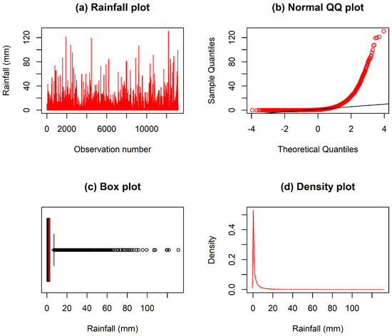
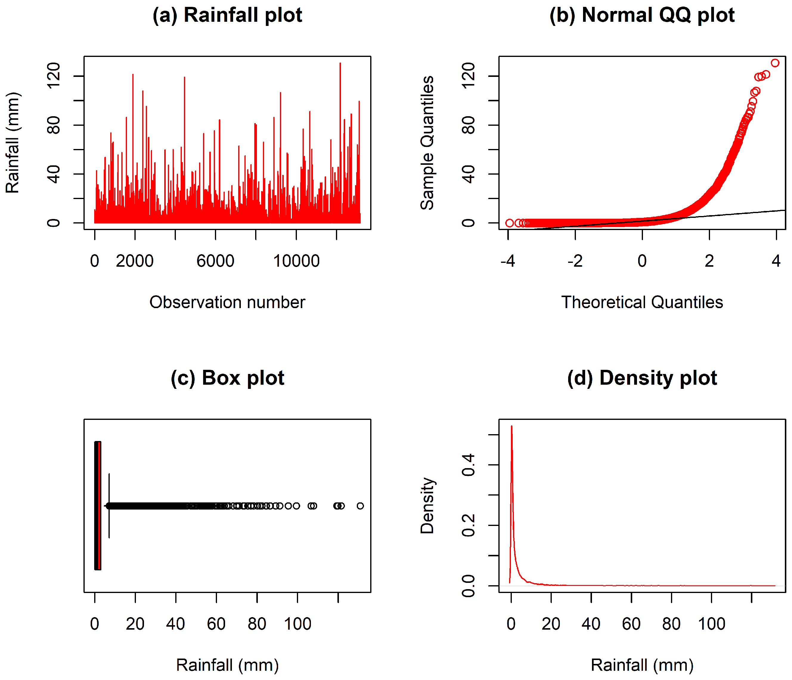
Figure 2 presents an analysis of rainfall data through four different plots. The time series plot in (a) vividly displays significant fluctuations in rainfall over time. The normal Q-Q plot in (b) shows a clear departure from a normal distribution, evidenced by a distinct S-shaped curve that points to a positively skewed distribution with heavy tails. This right skewness is further confirmed by the box plot in (c), which also highlights numerous outliers in the higher rainfall ranges. Finally, the density plot in (d) illustrates a sharp peak near zero and a long right tail, indicating that low rainfall is quite common, while high rainfall events are rare. Overall, the data is highly skewed, non-normal, and contains extreme values.

3.1. Time-Varying Threshold Selection Results

The threshold $u\left(t\right)$ is estimated as the conditional quantile of rainfall given the covariates, allowing it to vary with time and meteorological conditions. In essence, this means the threshold adapts over time based on changing weather conditions, rather than using a single fixed cutoff.

Table 2. Description of meteorological variables used in the analysis.

Variable	Description
T2M	Temperature at 2 m (°C)
T2M_MAX	Maximum temperature at 2 m (°C)
T2M_MIN	Minimum temperature at 2 m (°C)
PS	Surface pressure (kPa)
WS10M	Wind speed at 10 m (m/s)
WS2M	Wind speed at 2 m (m/s)
WS10M_MAX	Maximum wind speed at 10 m (m/s)
WS10M_MIN	Minimum wind speed at 10 m (m/s)
WS2M_MAX	Maximum wind speed at 2 m (m/s)
WS2M_MIN	Minimum wind speed at 2 m (m/s)
WD10M	Wind direction at 10 m (degrees)
WD2M	Wind direction at 2 m (degrees)
RH2M	Relative humidity at 2 m (%)
YEAR	Calendar year
DOY	Day of year (1–365/366)

provides a reference summary of all variables considered in the analysis.

A LASSO regression was first applied for variable selection. At the one-standard-error penalty (${\lambda }_{1se}$), LASSO regression retained six predictors: T2M_MAX, WS2M, WD2M, RH2M, WS2M_MAX, and WS2M_MIN. These variables reflect atmospheric moisture availability and near-surface wind dynamics, both of which are known drivers of extreme rainfall.

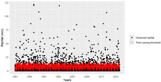
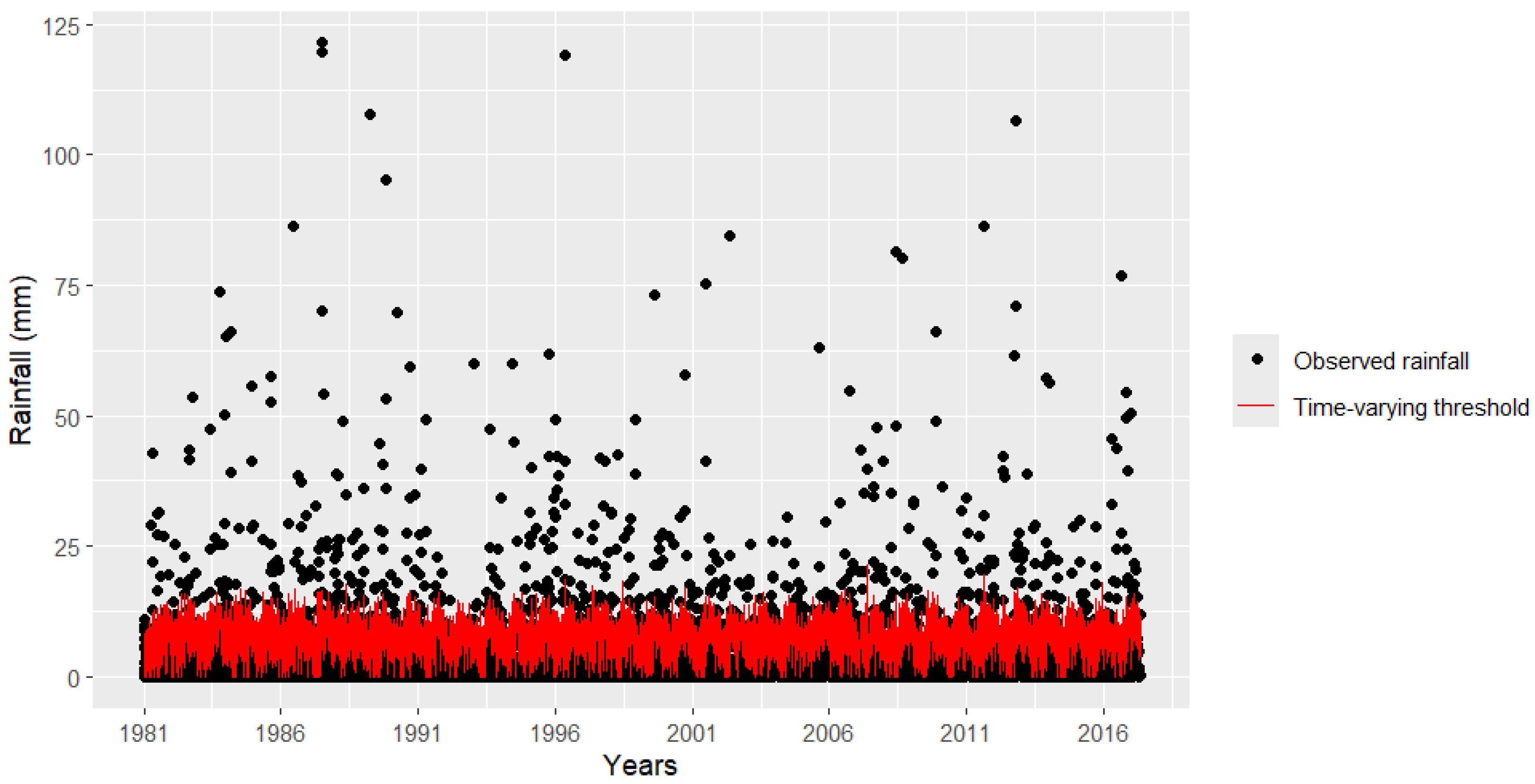
Using these selected predictors, a time-varying threshold was estimated at the 90th percentile ($\tau =0.90$) using quantile regression. The selection of the 90th percentile guarantees that the tail data is extreme enough to meet the theoretical requirements of the GPD while maintaining a sufficient sample size for stable model parameter estimation. Observations exceeding this conditional quantile were classified as extreme rainfall events. Figure 3 illustrates the estimated time-varying threshold alongside the observed rainfall. A total of 1050 exceedances above the time-varying threshold were identified in the training dataset, representing approximately 10% of the 10,537 observations. The POT framework requires approximately independent exceedances. Daily rainfall extremes can exhibit temporal clustering due to persistent storm systems. To address this, a standard runs declustering procedure was applied to the identified exceedances, with a minimum inter-exceedance gap of three days, following the approach of Davison and Smith [38]. The declustered series was used for GPD parameter estimation within each terminal node. This step ensures that successive exceedances belonging to the same storm event are treated as a single cluster maximum, thereby satisfying the independence assumption of the POT framework. Meteorological covariates are similarly expected to exhibit serial correlation; however, the tree-partitioning step conditions on covariate states, which mitigates residual dependence within each terminal node.

3.2. Time-Varying Threshold GP Regression Tree Model Fitting Results

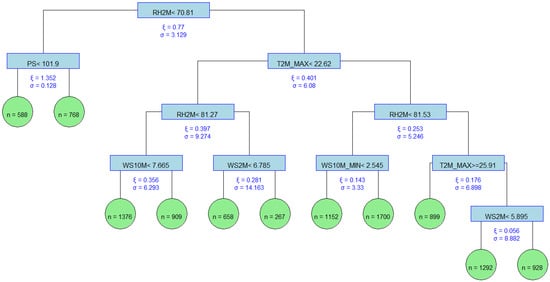
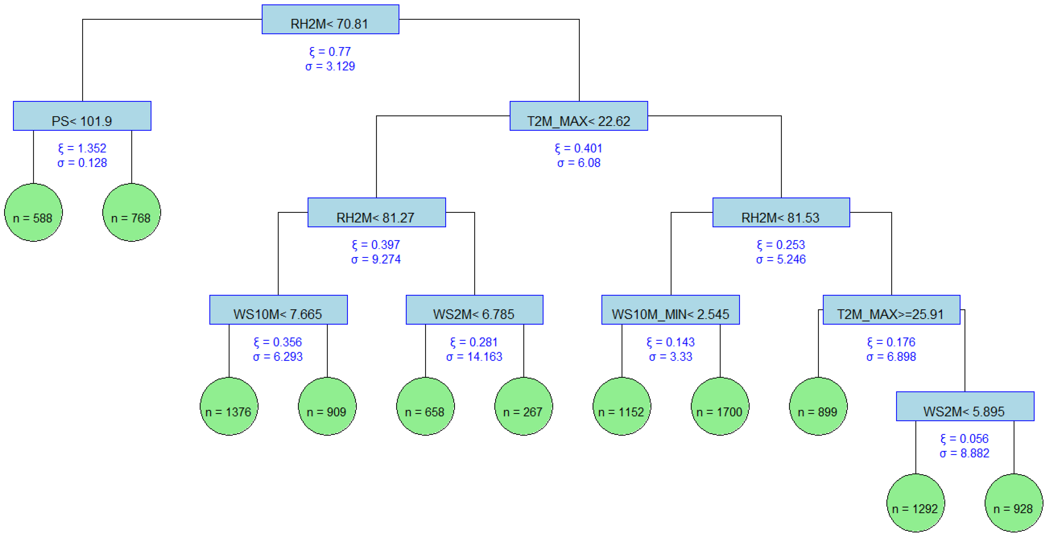
The fitted time-varying threshold GP regression tree in Figure 4 employs a likelihood-based recursive partitioning approach to identify covariate-driven subpopulations with homogeneous tail behaviour. In simpler terms, the fitted time-varying threshold GP regression tree model divides the data into groups whose extremes behave similarly, allowing distinct statistical relationships to be captured within each group. At each candidate split, the algorithm fits a GPD to the exceedances defined under the time-varying threshold selected in Figure 3 and selects the covariate and split point that minimise the GPD negative log-likelihood. The shape ($\xi$) and scale ($\sigma$) parameters printed on the internal nodes of Figure 4 represent the GPD estimates used during split evaluation.

In Figure 4, relative humidity at 2 m ($\mathrm{RH}2\mathrm{M}$) emerged as the primary splitting variable, partitioning the data at 70.81%. Subsequent divisions were based on surface pressure ($\mathrm{PS}=101.9$ kPa) and maximum temperature at 2 m ($\mathrm{T}2\mathrm{M}\_\mathrm{MAX}=22.62 °\mathrm{C}$), indicating that humidity, surface pressure, and temperature predominantly govern rainfall tail heterogeneity. In higher humidity regimes, additional splits on wind metrics ($\mathrm{WS}10\mathrm{M}$, $\mathrm{WS}2\mathrm{M}$, $\mathrm{WS}10\mathrm{M}\_\mathrm{MIN}$) further refined the tree, suggesting that low-level wind dynamics modulate the intensity of convective extremes. Variation in the ($\xi ,\sigma$) pairs across nodes reflects regime-dependent tail behaviour with larger $\xi$ values associated with heavier tails, while smaller $\xi$ values correspond to less extreme but still significant exceedances. This heterogeneity confirms that rainfall extremes exhibit distinct statistical structures across atmospheric states.

The configuration of the tree in Figure 4 is determined by three control parameters specified during model fitting: minsplit = 100, minbucket = 70, and cp = 0. The minsplit parameter stipulates that a node must contain at least 100 observations before it may be considered for splitting, ensuring statistical robustness in the splitting process. The minbucket parameter enforces that each terminal node must retain a minimum of 70 observations, providing stability in the estimation of the GPD parameters. Setting cp = 0 implies that no cost-complexity pruning was applied, allowing the tree to grow to its maximum size given the data and the specified splitting rules. As a result, the model retains all partitions identified through recursive likelihood optimisation, producing a comprehensive representation of covariate-driven heterogeneity in tail behaviour. Variables that fail to meet these criteria, or that do not contribute additional explanatory power once other splits have been made, will not be selected. The resulting tree in Figure 4 thus highlights only those variables that provide the strongest evidence of heterogeneity in the tail behaviour under the specified configuration.

3.3. Tree Pruning and Model Simplification

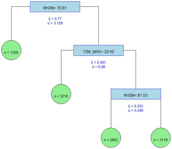
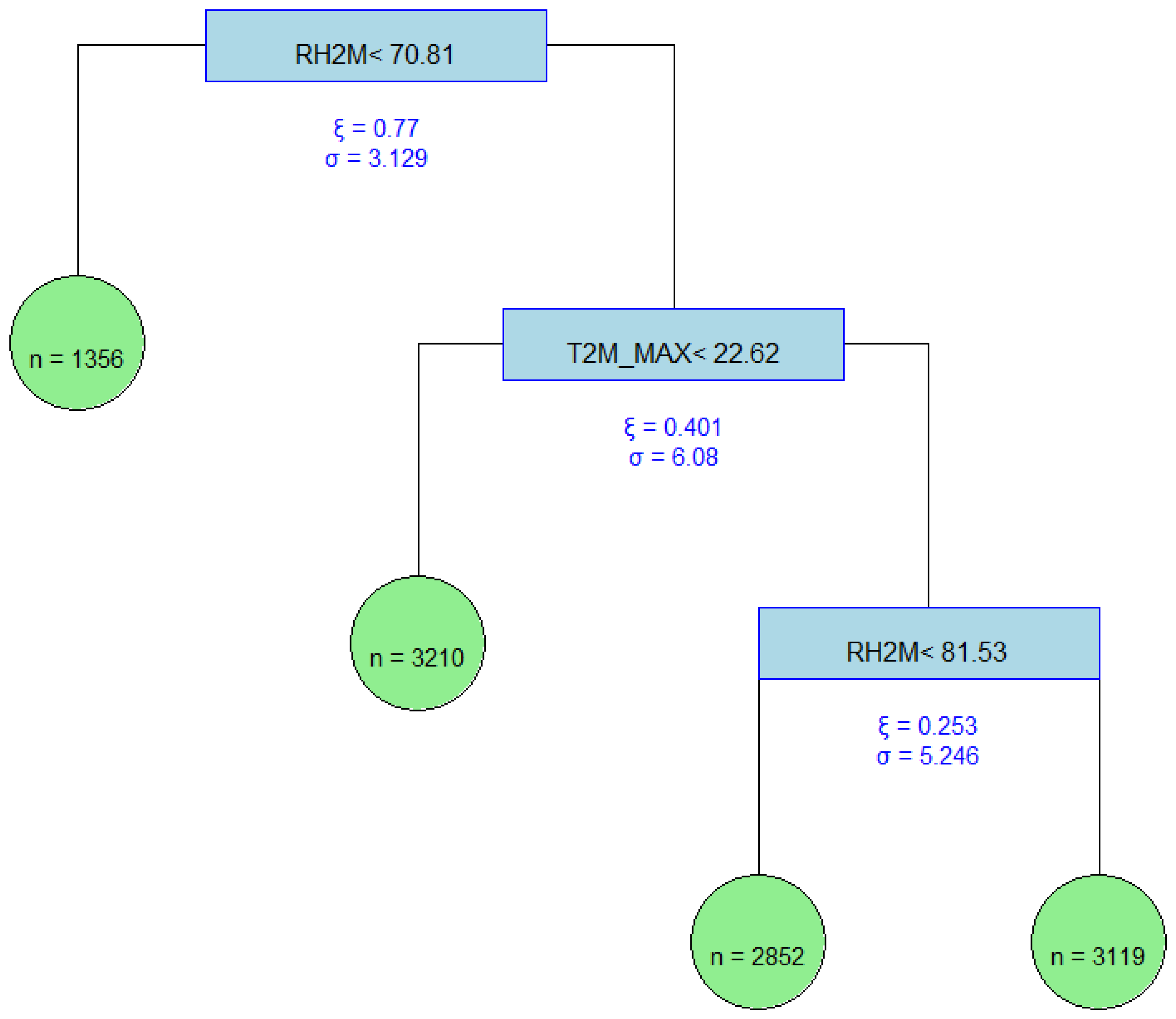
The pruned time-varying GP regression tree model presented in Figure 5 constitutes a refined and parsimonious representation of the maximal tree model, obtained through a principled penalisation framework. Pruning was performed by minimising the penalised criterion $C_A\left(G\right)$ in Equation (4), removing branches that offered negligible reductions in GPD deviance. This procedure enhances model interpretability and generalisability by retaining only statistically meaningful partitions.

In Figure 5 the root node splits on relative humidity at 2 m ($\mathrm{RH}2\mathrm{M}=70.81\%$), separating dry from humid regimes. The dry branch ($\mathrm{RH}2\mathrm{M}<70.81\%$) forms a homogeneous terminal node ($n=1356$), while the humid branch undergoes further splits on maximum temperature ($\mathrm{T}2\mathrm{M}\_\mathrm{MAX}=22.62 °\mathrm{C}$) and relative humidity ($\mathrm{RH}2\mathrm{M}=81.53\%$). This results in three additional subpopulations representing cool–humid, moderately humid–warm, and highly humid–warm regimes, with sample sizes of 3210, 2852, and 3119, respectively.

These results in Figure 5 reveal four distinct rainfall regimes: dry low humidity, cool–humid, moderately humid–warm, and highly humid–warm, each exhibiting unique tail characteristics. Drier regimes are associated with lighter tails, reflecting limited convective activity, while humid and warmer regimes display progressively heavier tails indicative of intense convective rainfall. The pruned tree model presented in Figure 4 effectively condenses complex atmospheric variability into a compact, interpretable structure that preserves explanatory strength. By linking rainfall extremes to specific meteorological regimes, it offers a robust framework for understanding and characterising the atmospheric drivers of extreme rainfall and their implications for environmental risk assessment.

3.4. Model Evaluation Results

This section presents a comparative evaluation of three models: the proposed time-varying threshold GP regression tree model, the static threshold GP regression tree model, and the time-varying threshold GPD.

Table 3. Comparative performance of the proposed time-varying threshold GP regression tree model against two benchmark models on the training and testing datasets.

Benchmark Model	BIC	Log-Likelihood
Training data
Time-varying threshold GP regression tree	5484.592	−2705.245
Static threshold GP regression tree	6822.345	−3179.606
Time-varying threshold GPD	7936.860	−3961.474
Testing data
Time-varying threshold GP regression tree	5473.503	−2736.418
Static threshold GP regression tree	6753.044	−3215.872
Time-varying threshold GPD	–	–

summarises the performance of the three benchmark models on both training and testing datasets. The time-varying threshold GP regression tree model consistently outperforms the alternatives, achieving the lowest BIC and highest log-likelihood across both datasets, which indicates an optimal balance between fit and complexity and demonstrates robust generalisability, as shown in Table 3. A smaller BIC value indicates a more efficient model because it rewards a better fit while penalising unnecessary complexity, thereby discouraging overfitting. The static threshold GP regression tree model performs substantially worse. It was fitted using a fixed threshold of 8.3 mm, determined using the mean residual life plot and threshold stability plots. This reflects the inability of the static threshold GP regression tree model to accommodate temporal variability and covariate-driven heterogeneity in extreme rainfall. The time-varying threshold GPD, while more flexible than the static tree model, remains inferior to the time-varying GP regression tree model. An attempt was made to evaluate the time-varying threshold GPD on the test set by computing its out-of-sample log-likelihood using the parameters estimated on the training set. However, because the time-varying threshold GPD is a globally parametric model with fixed functional forms for the threshold and tail parameters, its out-of-sample likelihood is highly sensitive to covariate values falling outside the training range, resulting in numerically unstable evaluations for the test period that includes the atypical April 2022 Durban flood event. This instability means direct BIC comparison with the regression tree on the test set is not methodologically sound for this model. We acknowledge this as an important limitation: direct out-of-sample likelihood comparison between the GPD and the tree-based models requires a fully non-parametric or cross-validated procedure that we recommend as a direction for future work. The results confirm that incorporating both time-varying thresholds and covariate-dependent partitioning yields an improved model for extreme rainfall analysis.

3.5. Return Levels Estimation

This section presents the return levels estimated for terminal nodes to complement the structural interpretation of the pruned time-varying GP regression tree. Return levels indicate the magnitude of daily rainfall expected to be exceeded, on average, once every T years, where T denotes the return period. These estimates provide a direct link between the statistical tail behaviour captured by the model and the practical assessment of flood risk under varying climatic conditions. Before interpreting return levels, it is important to note that local thresholds were independently estimated within each terminal node, reflecting the node-specific distribution of rainfall as shown in

Table 4. Local thresholds (98th percentile) and exceedances for each terminal node.

Terminal Node	Sample Size	Local Threshold (mm)	Exceedances
1	1356	5.756	28
2	3210	32.882	65
3	2852	11.049	58
4	3119	26.210	63

. These thresholds correspond to the 98th percentile of daily rainfall within the node, computed using only the observations assigned to that node. The procedure involved the following steps:

(a)

Identify the observations that belong to each terminal node in the pruned tree model.

(b)

Compute the 98th percentile rainfall value for each node to serve as the local threshold.

(c)

Count the number of exceedances above this local threshold that provide the data to fit the GPD within the node.

This approach ensures that extreme value analysis is tailored to the specific characteristics of each regime, rather than imposing a single global threshold across all observations.

With these node-specific thresholds in place, the return levels summarise the magnitude of daily rainfall expected to be exceeded on average once every T years within each node.

Table 5. Return level estimates with 95% confidence intervals (CI) for each terminal node.

Terminal Node	$\mathit{\xi }$ (95% CI)	$\mathit{\sigma }$	Return Period (Years)	Return Level (95% CI)
1	0.492 ($-0.126$; 1.109)	2.558	10	14.84 (10.47; 19.56)
			20	19.52 (12.43; 28.36)
			50	27.45 (15.15; 45.71)
			100	35.11 (17.13; 65.09)
			150	40.41 (18.11; 79.88)
			200	44.59 (18.90; 93.97)
2	0.036 ($-0.267$; 0.339)	4.411	10	31.60 (15.60; 47.61)
			20	35.22 (14.05; 56.39)
			50	40.14 (10.76; 69.51)
			100	43.97 (7.28; 80.66)
			150	46.26 (4.82; 87.69)
			200	47.90 (2.89; 92.91)
3	$-0.197$ ($-0.455$; 0.061)	30.742	10	122.09 (69.26; 174.92)
			20	130.63 (67.70; 193.56)
			50	140.26 (64.03; 216.49)
			100	146.47 (60.41; 232.54)
			150	149.74 (58.06; 241.41)
			200	151.90 (56.32; 247.48)
4	$-0.079$ ($-0.356$; 0.197)	11.271	10	67.29 (39.67; 94.90)
			20	72.69 (38.11; 107.27)
			50	79.40 (34.73; 124.06)
			100	84.16 (31.29; 137.02)
			150	86.82 (28.96; 144.68)
			200	88.66 (27.17; 150.15)

presents the estimated return levels for each terminal node of a pruned tree model in Figure 5, along with 95% confidence intervals. These estimates allow a clear interpretation of the climatic regimes governing extreme rainfall in Durban.

The GPD parameter estimates presented in Table 5 highlight systematic differences in tail behaviour and variability across the four terminal nodes. The shape parameter $\xi$ primarily governs tail heaviness, indicating whether the distribution of exceedances is light-tailed, heavy-tailed, or bounded, while the scale parameter $\sigma$ quantifies the dispersion of exceedances within the node. Together, these parameters determine the magnitude, variability, and predictability of extreme rainfall events, and explain the rate at which return levels increase with longer return periods.

Terminal node 1 is characterised by a positive shape parameter ($\xi =0.492$) and a relatively small scale parameter ($\sigma =2.558$). The positive point estimate of the shape parameter suggests a tendency towards heavier-tailed behaviour, consistent with a Fréchet-type distribution, although the wide confidence interval spanning negative to positive values means this characterisation must be treated with caution. Noting this uncertainty, the data within this node appears somewhat more susceptible to large rainfall extremes than nodes with near-zero or negative point estimates. This behaviour is reflected in the steady increase in return levels, which rise from 14.84 mm/day at the 10-year return period to 44.59 mm/day at 200 years. The widening confidence intervals at longer return periods further emphasise the uncertainty inherent in heavy-tailed distributions, where rare events exert a disproportionate influence on parameter estimation. Terminal node 2 displays a shape parameter close to zero ($\xi =0.036$) and a moderate scale parameter ($\sigma =4.411$). A near-zero shape value corresponds to a Gumbel distribution, representing an intermediate case between heavy and light tails. This suggests that while extreme rainfall events are possible, their probability diminishes more rapidly than in Terminal node 1. The moderate scale parameter indicates a wider spread of rainfall magnitudes compared to Terminal node 1, reflecting greater variability in extremes. Return levels increase gradually with return period, reaching 47.90 mm/day at 200 years, and relatively wider confidence intervals suggest that the extremes in this node are less predictable and less uncertain than those in Terminal node 1.

Terminal node 3 is defined by a negative shape parameter ($\xi =-0.197$) and the largest scale parameter across all nodes ($\sigma =30.742$). The negative point estimate of the shape parameter is suggestive of a light-tailed, Weibull-type distribution and a potential finite upper bound on extremes, though the confidence interval again includes zero and this characterisation is not statistically confirmed. However, the very large scale parameter denotes a substantial spread in exceedance values, producing high variability within this bounded range. As a result, return levels are extremely large, with the 200-year return level reaching 151.90 mm/day, but their growth slows as the return period increases. This combination suggests that extremes in Terminal node 3 are highly variable, leading to large but ultimately capped magnitudes. Terminal node 4 also exhibits a slightly negative shape parameter ($\xi =-0.079$) alongside a moderate scale parameter ($\sigma =11.271$). The negative shape again points to a Weibull distribution, though the tail is less strongly bounded than in Terminal node 3. This indicates that extreme rainfall values are somewhat limited in magnitude, with return levels increasing more slowly as the return period lengthens. The moderate scale parameter reflects a balanced degree of variability, producing a 200-year return level of 88.66 mm/day. Compared with the other nodes, Terminal node 4 represents an intermediate case, neither strongly bounded nor excessively variable, suggesting a relatively stable regime of extreme rainfall behaviour.

The 95% confidence intervals for the shape parameter ($\xi$) in all four terminal nodes include zero. This implies that, based on available data, there is insufficient statistical evidence to conclude that the shape parameter is significantly different from zero in any of the four nodes. Accordingly, the Gumbel (exponential-tail) model cannot be formally rejected for any regime. The point estimates of $\xi$ nonetheless vary across nodes and are interpreted as indicative of regime-specific tail tendencies, subject to the caveat that these differences are not statistically confirmed at conventional significance levels.

4. Discussion

The findings of the study, as presented in the Results section, provide a substantive contribution to the field of extreme value analysis, particularly in the context of meteorological modelling in South Africa. The application of the time-varying GP regression tree model has not only successfully addressed the research aim of accurately modelling extreme rainfall but has also yielded profound insights into the underlying meteorological mechanisms governing such events. The superior performance of the time-varying threshold GP regression tree model, as demonstrated by the evaluation metrics in Table 3, establishes its efficacy and justifies its utility as a robust alternative to traditional statistical and machine learning benchmarks. These findings directly support the application of GP regression trees, which is scarce in the literature, thereby bridging a critical research gap and validating the proposed methodological approach.

The time-varying threshold GP regression tree model elucidates the atmospheric mechanisms underpinning Durban’s rainfall extremes. The differentiated tail behaviour across terminal nodes reveals distinct climatological regimes: for example, high-humidity, low-pressure conditions correspond to intense convective events and cyclonic incursions, whereas moderate-humidity, stable-pressure conditions align with more typical seasonal rainfall. Such stratification demonstrates that extreme rainfall in Durban is not a single homogeneous process, but a suite of atmospheric pathways. This is consistent with and extends earlier EVT studies of Singirankabo and Iyamuremye [17] and Musayidizi [21] that have generally treated rainfall extremes as stationary phenomena, and it resonates with hybrid approaches proposed by Velthoen et al. [31] and Gnecco et al. [32], which call for covariate-sensitive tail modelling.

Furthermore, the time-varying threshold GP regression tree model offers a nuanced understanding of the causal relationships underpinning extreme rainfall and extends the work of Farkas et al. [34,35,36] that considered a constant threshold. The hierarchical structure of the model, particularly the splits based on covariates like relative humidity, surface pressure, and temperature, illuminates the distinct meteorological pathways that culminate in heavy rainfall. This mechanistic insight extends beyond mere modelling accuracy, providing a physically interpretable framework for understanding how varying atmospheric conditions interact to drive extreme events in the Durban metropolitan area. For example, the identification of specific meteorological regimes, such as those associated with high humidity and low-pressure systems, provides a detailed narrative of the conditions conducive to severe rainfall.

The practical implications of these results for modelling and risk management in Durban are substantial. The capacity of the time-varying threshold GP regression tree model to estimate return levels, as detailed in Section 3.5, provides stakeholders with a probabilistic measure of extreme event likelihood, which is an invaluable tool for urban planning, infrastructure design, and disaster preparedness. By identifying the meteorological preconditions for different rainfall-generating processes, policymakers and risk managers can develop more targeted and effective mitigation strategies. The ability to differentiate between the risks associated with various atmospheric regimes allows for a more granular approach to climate resilience, moving beyond generic flood warnings to a more scientifically grounded system of risk assessment. Ultimately, this research offers a tangible and actionable framework for enhancing the city’s capacity to manage the escalating risks associated with climate variability.

5. Conclusions

This study successfully developed and validated a robust, non-stationary framework for modelling extreme rainfall in the Durban metropolitan area through the proposed time-varying threshold GP regression tree model. By integrating extreme value theory with a machine learning technique, the model effectively addressed the limitations of traditional stationary approaches, capturing the heterogeneous and non-stationary nature of high-intensity rainfall events under dynamic atmospheric conditions. The central contribution of this research is the formulation of the time-varying threshold GP regression tree model, which demonstrated superior predictive performance compared to both the static threshold GP regression tree and the time-varying GPD benchmark models. This was evidenced by consistently lower BIC values and higher log-likelihoods across both training and testing datasets, indicating an optimal balance between model complexity, fit, and generalisability.

Beyond predictive accuracy, the model provides an interpretable framework for understanding the drivers of extreme rainfall. By partitioning rainfall data based on meteorological covariates such as relative humidity and maximum temperature, the model identified distinct atmospheric regimes. Within each terminal node, regime-specific GPD parameters quantified the scale and tail behaviour of extremes, confirming that prevailing meteorological conditions strongly influence them. The framework offers practical utility for climate resilience and disaster risk management. Estimation of regime-specific return levels enables more informed planning and design of stormwater infrastructure, flood defences, and urban development strategies. By attributing extreme rainfall to interpretable regimes, the model facilitates targeted adaptation measures and risk mitigation in coastal urban environments.

The findings of this study also provide a foundation for future research.

(a)

Future work could extend the current framework into a spatio-temporal Generalised Pareto regression tree that simultaneously captures spatial dependence, temporal dynamics, and time-varying threshold behaviour of rainfall extremes across multiple locations. Such an extension would enhance the model’s ability to represent evolving regional patterns of extreme rainfall and improve both the spatial generalisability and temporal adaptability of predictions.

(b)

The integration of Generalised Pareto regression tree model with ensemble or boosting methods such as Gradient Boosting Extreme Value models, Extremal Random Forests, or Bayesian Additive Regression Trees could strengthen predictive stability, reduce model uncertainty, and improve performance in out-of-sample forecasting.

(c)

Coupling the GP regression tree framework with bias-corrected climate model projections, such as CMIP6 datasets, would enable probabilistic projections of future extreme rainfall risk under various climate scenarios. This approach could provide critical insights for long-term adaptation planning and infrastructure design.

(d)

Future research should undertake a systematic comparison between the proposed time-varying GP regression tree and other hybrid or ensemble-based extreme value models, such as Gradient Boosting Extreme Value models, Extremal Random Forests, and Bayesian Additive Regression Trees. Such a comparative evaluation would help determine the relative strengths and limitations of each approach in terms of predictive accuracy, interpretability, and uncertainty quantification, thereby providing deeper insights into model robustness and suitability for operational extreme-event forecasting.

References

- Nhamo, G.; Chapungu, L.; Mutanda, G.W. Trends and impacts of climate-induced extreme weather events in South Africa (1920–2023). Environ. Dev. 2025, 55, 101183. [Google Scholar] [CrossRef] [Scilit]
- Ebi, K.L.; Vanos, J.; Baldwin, J.W.; Bell, J.E.; Hondula, D.M.; Errett, N.A.; Hayes, K.; Reid, C.E.; Saha, S.; Spector, J.; et al. Extreme weather and climate change: Population health and health system implications. Annu. Rev. Public Health 2021, 42, 293–315. [Google Scholar] [CrossRef] [Scilit] [PubMed]
- Myhre, G.; Alterskjær, K.; Stjern, C.W.; Hodnebrog, Ø.; Marelle, L.; Samset, B.H.; Sillmann, J.; Schaller, N.; Fischer, E.; Schulz, M.; et al. Frequency of extreme precipitation increases extensively with event rareness under global warming. Sci. Rep. 2019, 9, 16063. [Google Scholar] [CrossRef] [Scilit] [PubMed]
- Bopape, M.M.; Keebine, G.; Ndarana, T.; Mbokodo, I.L.; Hlahane, K.; Motshegwa, T.; Amha, Y.; Ogega, O.M.; Mfopa, C.; Mahlobo, D.D.; et al. Weather related disasters in South Africa from 1980 to 2023. Environ. Dev. 2025, 56, 101254. [Google Scholar] [CrossRef] [Scilit]
- South African History Online. At Least 100 People Drown in a Flood at Laingsburg. South African History Online. 16 March 2011. Available online: https://sahistory.org.za/dated-event/least-100-people-drown-flood-laingsburg (accessed on 21 October 2025).
- Grab, S.W.; Nash, D.J. A new flood chronology for KwaZulu-Natal (1836–2022): The April 2022 Durban floods in historical context. S. Afr. Geogr. J. 2024, 106, 476–497. Available online: https://hdl.handle.net/10520/ejc-sageo_v106_n4_a476 (accessed on 25 May 2026). [CrossRef] [Scilit]
- Pinto, I.; Zachariah, M.; Wolski, P.; Landman, S.; Phakula, V.; Maluleke, W.; Bopape, M.-J.; Engelbrecht, C.; Jack, C.; McClure, A.; et al. Climate Change Exacerbated Rainfall Causing Devastating Flooding in Eastern South Africa. World Weather Attribution. 2022. Available online: https://www.worldweatherattribution.org/climate-change-exacerbated-rainfall-causing-devastating-flooding-in-eastern-south-africa/ (accessed on 25 May 2026).
- Jury, M.R.; Lindesay, J.A.; Wittmeyer, I. Flood episodes in central South Africa from satellite and ECMWF data. S. Afr. J. Sci. 1993, 89, 263–269. [Google Scholar]
- Presidential Climate Commission. A Critical Analysis of the Impacts of and Responses to the April–May 2022 Floods in KwaZulu-Natal; Republic of South Africa: Rosebank, South Africa, 2023; Available online: https://pccommissionflo.imgix.net/uploads/images/PCC-Brief-KZN-Floods.pdf (accessed on 23 October 2025).
- Martel, J.-L.; Brissette, F.P.; Lucas-Picher, P.; Troin, M.; Arsenault, R. Climate change and rainfall intensity–duration–frequency curves: Overview of science and guidelines for adaptation. J. Hydrol. Eng. 2021, 26, 03121001. [Google Scholar] [CrossRef] [Scilit]
- Merz, B.; Kuhlicke, C.; Kunz, M.; Pittore, M.; Babeyko, A.; Bresch, D.N.; Domeisen, D.I.V.; Feser, F.; Koszalka, I.; Kreibich, H.; et al. Impact forecasting to support emergency management of natural hazards. Rev. Geophys. 2020, 58, e2020RG000704. [Google Scholar] [CrossRef] [Scilit]
- Wani, O.A.; Mahdi, S.S.; Yeasin, M.; Kumar, S.S.; Gagnon, A.S.; Danish, F.; Al-Ansari, N.; El-Hendawy, S.; Mattar, M.A. Predicting rainfall using machine learning, deep learning, and time series models across an altitudinal gradient in the North-Western Himalayas. Sci. Rep. 2024, 14, 27876. [Google Scholar] [CrossRef] [Scilit]
- Xuan, Z.-y.; Zheng, F.; Zhu, J. The effectiveness of machine learning methods in the nonlinear coupled data assimilation. Geosci. Lett. 2024, 11, 43. [Google Scholar] [CrossRef] [Scilit]
- Coles, S.; Bawa, J.; Trenner, L.; Dorazio, P. An Introduction to Statistical Modeling of Extreme Values; Springer: London, UK, 2001. [Google Scholar]
- Barakat, H.M.; Khaled, O.M.; Nigm, E.S.M. Statistical Techniques for Modelling Extreme Value Data and Related Applications; Cambridge Scholars Publishing: London, UK, 2019. [Google Scholar]
- Phoophiwfa, T.; Chomphuwiset, P.; Prahadchai, T.; Park, J.-S.; Apichottanakul, A.; Theppang, W.; Busababodhin, P. Employing the generalized Pareto distribution to analyze extreme rainfall events on consecutive rainy days in Thailand’s Chi watershed: Implications for flood management. Hydrol. Earth Syst. Sci. 2024, 28, 801–816. [Google Scholar] [CrossRef] [Scilit]
- Singirankabo, E.; Iyamuremye, E. Modelling extreme rainfall events in Kigali city using generalized Pareto distribution. Meteorol. Appl. 2022, 29, e2076. [Google Scholar] [CrossRef] [Scilit]
- Sunday, S.B.; Agog, N.S.; Magdalene, P.; Mubarak, A.; Anyam, G.K. Modeling extreme rainfall in Kaduna using the generalised extreme value distribution. Sci. World J. 2020, 15, 73–77. [Google Scholar]
- McBride, C.M.; Kruger, A.C.; Dyson, L. Changes in extreme daily rainfall characteristics in South Africa: 1921–2020. Weather Clim. Extrem. 2022, 38, 100517. [Google Scholar] [CrossRef] [Scilit]
- Sikhwari, T.; Nethengwe, N.; Sigauke, C.; Chikoore, H. Modelling of extremely high rainfall in Limpopo Province of South Africa. Climate 2022, 10, 33. [Google Scholar] [CrossRef] [Scilit]
- Musayidizi, J.D. Peak-over-threshold analysis of extreme Rainfall in the North Western Region of Rwanda. Ph.D. Thesis, University of Rwanda, Kigali, Rwanda, 2022. [Google Scholar]
- Tugrul, T.; Oruc, S.; Gunes, B. Quantifying future rainfall extremes in Türkiye: A CMIP6 ensemble approach with statistical downscaling. Acta Geophys. 2025, 73, 3477–3494. [Google Scholar] [CrossRef] [Scilit]
- Garba, I.; Abdourahamane, Z.S. Extreme rainfall characterisation under climate change and rapid population growth in the city of Niamey, Niger. Heliyon 2023, 9, e13326. [Google Scholar] [CrossRef] [Scilit] [PubMed]
- Patil, K.R.; Doi, T.; Behera, S.K. Predicting extreme floods and droughts in East Africa using a deep learning approach. npj Clim. Atmos. Sci. 2023, 6, 108. [Google Scholar] [CrossRef] [Scilit]
- Kagabo, J.; Kattel, G.R.; Kazora, J.; Shangwe, C.N.; Habiyakare, F. Application of machine learning algorithms in predicting extreme rainfall events in Rwanda. Atmosphere 2024, 15, 691. [Google Scholar] [CrossRef] [Scilit]
- Ebtehaj, I.; Bonakdari, H. CNN vs. LSTM: A comparative study of hourly precipitation intensity prediction as a key factor in flood forecasting frameworks. Atmosphere 2024, 15, 1082. [Google Scholar] [CrossRef] [Scilit]
- Saubhagya, S.; Tilakaratne, C.; Lakraj, P.; Mammadov, M. Granger Causality-Based Forecasting Model for Rainfall at Ratnapura Area, Sri Lanka: A Deep Learning Approach. Forecasting 2024, 6, 1124–1151. [Google Scholar] [CrossRef] [Scilit]
- Mdegela, L.; Municio, E.; De Bock, Y.; Luhanga, E.; Leo, J.; Mannens, E. Extreme rainfall event classification using machine learning for Kikuletwa River floods. Water 2023, 15, 1021. [Google Scholar] [CrossRef] [Scilit]
- Ogunniyi, J.A.; Abd Elbasit, M.A.M.; Obagbuwa, I.C. Monthly rainfall prediction for different climatic zones in South Africa for 2024 using a random forest model. Edelweiss Appl. Sci. Technol. 2024, 8, 1805–1827. Available online: https://learning-gate.com/index.php/2576-8484/article/view/2347/910 (accessed on 25 May 2026). [CrossRef] [Scilit]
- Anco-Valdivia, J.; Valencia-Félix, S.; Vigil, A.J.E.; Anco, G.; Booker, J.; Juarez-Quispe, J.; Rojas-Chura, E. Precipitation Return Period Estimation Using Random Forest: A Comparative Analysis with Probability Density Functions Using Outdated Weather Station Data. Preprints 2024, 2024110492. Available online: https://www.preprints.org/manuscript/202411.0492/v1 (accessed on 25 May 2026).
- Velthoen, J.; Dombry, C.; Cai, J.-J.; Engelke, S. Gradient boosting for extreme quantile regression. Extremes 2023, 26, 639–667. [Google Scholar] [CrossRef] [Scilit]
- Gnecco, N.; Terefe, E.M.; Engelke, S. Extremal random forests. J. Am. Stat. Assoc. 2024, 119, 3059–3072. [Google Scholar] [CrossRef] [Scilit]
- Grazzini, F.; Dorrington, J.; Grams, C.M.; Craig, G.C.; Magnusson, L.; Vitart, F. Improving forecasts of precipitation extremes over northern and central Italy using machine learning. Q. J. R. Meteorol. Soc. 2024, 150, 3167–3181. [Google Scholar] [CrossRef] [Scilit]
- Farkas, S.; Lopez, O.; Thomas, M. Cyber Claim Analysis Through Generalized Pareto Regression Trees with Applications to Insurance. 2020. Available online: https://hal.science/hal-02118080 (accessed on 15 October 2025).
- Farkas, S.; Lopez, O.; Thomas, M. Cyber claim analysis using Generalized Pareto regression trees with applications to insurance. Insur. Math. Econ. 2021, 98, 92–105. [Google Scholar] [CrossRef] [Scilit]
- Farkas, S.; Heranval, A.; Lopez, O.; Thomas, M. Generalized Pareto regression trees for extreme event analysis. Extremes 2024, 27, 437–477. [Google Scholar] [CrossRef] [Scilit]
- IOL. Durban Floods ‘Most Catastrophic Natural Disaster’ to Ever Hit KZN–Study. 2024. Available online: https://www.iol.co.za/news/environment/durban-floods-most-catastrophic-natural-disaster-to-ever-hit-kzn-study-5d164bd0-9110-4379-9a3e-c9004fb34875 (accessed on 14 October 2025).
- Davison, A.C.; Smith, R.L. Models for exceedances over high thresholds. J. R. Stat. Soc. Ser. B Stat. Methodol. 1990, 52, 393–425. [Google Scholar] [CrossRef] [Scilit]
Disclaimer/Publisher’s Note: The statements, opinions and data contained in all publications are solely those of the individual author(s) and contributor(s) and not of MDPI and/or the editor(s). MDPI and/or the editor(s) disclaim responsibility for any injury to people or property resulting from any ideas, methods, instructions or products referred to in the content. |
© 2026 by the authors. Licensee MDPI, Basel, Switzerland. This article is an open access article distributed under the terms and conditions of the Creative Commons Attribution (CC BY) license.