


Abstract
Simulation studies of surplus electricity in sugarcane cogeneration almost universally assume stable nominal operation, and the sector literature qualitatively acknowledges that many surplus projects underperform; however, this discrepancy has not been systematically quantified against multiyear operational records. Using daily records from seven harvest seasons (2010–2016; 931 valid days) of a Cuban low-pressure sugar mill and the previously published simulation of its own thermal scheme (Termoazúcar STA 4.1), this study quantifies the discrepancy through the Energy Performance Gap (EPG) framework adapted from building science. The export shortfall relative to the simulated baseline ranged from 19.0% to 49.3% per harvest (38.1% aggregated over 2010–2015; 12,835 MWh unrealized) and reached 28.9% for the five-mill provincial aggregate. The gap does not arise from idle capacity—availability is 0.98–1.00, and industrial demand matches the simulated value—but from conversion, with a cane-weighted generation deficit of 5.46 kWh/t (%). Plant steam records proved to be accounting allocations based on fixed coefficients and cannot support correlation-based inference; what they document independently is a contiguous start-of-season regime with pressure-reducing valves in service (39 days of a single harvest), during which specific generation was 11.9 kWh/t lower at statistically identical milling rates (26.15 vs. 38.06 kWh/t; ). No interannual trend was detected (Mann–Kendall, ), although statistical power is limited, at . A Monte Carlo characterization of the parametric uncertainty of the simulated baseline (boiler efficiency %, turbine isentropic efficiency %, and bagasse moisture percentage points) shows that the existence of the gap is robust—the probability of no gap is, at most, 1.1%, even under worst-case uniform perturbations—while widening the intensity-level discount interval to [0.57; 0.93]; a start-of-season depression in specific generation recurs in four of the six estimable harvests, of which the 2015 reducer regime is the most severe instance. As case-specific correction tools, operational discount factors of 0.71 (95% block-bootstrap CI [0.68; 0.75]) for export intensity and 0.62 for total seasonal energy are derived; the underlying procedure, rather than the numerical values, is proposed as transferable.
1. Introduction
Cogeneration using bagasse constitutes the energetic backbone of the sugar agroindustry, one of the most mature renewable bioelectricity pathways worldwide, and one of the lowest-cost decarbonization levers available to sugar-producing economies. More than one hundred countries produce sugarcane, and electricity generation from bagasse already represents a relevant contribution to national energy matrices in Brazil, India, Thailand, Mauritius, and Cuba, among others, where the surplus electricity exported to the grid has become a third product alongside sugar and ethanol [1,2,3].
Research in the sector has concentrated on estimating the surplus-electricity potential under different technological reconfigurations: replacement of back-pressure steam turbines (BPSTs) by extraction–condensing steam turbine (CEST) schemes, which can quadruple the surplus [4]; recovery of sugarcane straw as a complementary fuel, with increases of up to 30% [5]; introduction of high-pressure steam generators operating up to 105 bar and 525 °C [3]; hybridization with vinasse biogas and excess bagasse [6]; and biomass-integrated gasification combined cycles (BIGCC) [7]. Recent reviews consolidate this range of strategies and emphasize the reduction in bagasse moisture content and improvements in boiler efficiency as cross-cutting operational levers [8,9].
The dominant tool for quantifying these potentials is the simulation of mass and energy balances, frequently accompanied by exergy and thermoeconomic analyses. Exergy diagnostics of sugar mills in Aspen Plus locate the highest exergy destruction in the cogeneration system, with the boiler identified as the most irreversible component [10,11,12], a conclusion replicated through exergoenvironmental [13], advanced exergoeconomic [14], and model-plant studies from different countries [15,16].
Thermal integration through pinch analysis has demonstrated, since the seminal works of the methodology [17], that reducing process-steam demand—from about 400–550 to 280–300 kg per ton of cane under advanced technology—releases bagasse for electricity export [3,18], and the combination of pinch and exergy analysis has even been applied to real operational data from sugarcane cogeneration systems [19]. Added to this are the thermoeconomic optimization of operating modes [20,21], life-cycle assessment of cogeneration configurations [22], and the quantification of parametric improvements without capital investment [23].
For the low-pressure sugar-mill fleet of Cienfuegos Province (Cuba), this pathway was quantified with the Termoazúcar thermoenergetic balance simulator (STA 4.1), reporting potential increases of 12–50% in the electricity sold to the National Electric Power System (SEN) while maintaining the same cane throughput [24,25,26].
Much of this literature shares an assumption that is rarely made explicit: stable nominal operation. Both the baseline and the improved cases are simulated at potential milling capacity, under continuous operating conditions and design parameters, such that the baseline, itself, is an idealization of the existing thermal scheme rather than a representation of its real operation; consequently, both the baseline and the improvement potential may be systematically overestimated relative to what is operationally achievable.
The sector acknowledges this risk qualitatively: a recent review documents that numerous attempts to increase surplus electricity generation—including biomass-integrated gasification combined cycle (BIGCC) technology—have failed at both pilot and industrial scale [27]. However, quantitative antecedents remain limited to agronomic–industrial benchmarking, exergy diagnostics built entirely upon simulation [10], or isolated equipment validations against spot measurements [28]: to the best of the authors’ knowledge, no published study has systematically confronted the simulated potential of a sugarcane cogeneration scheme along with its multiyear daily operational record.
This discrepancy between predicted and actual performance has instead been the subject of a mature body of literature in building science, where it is termed the Energy Performance Gap (EPG). The framework proposed by de Wilde [29] defines it as the difference between the energy computed at the design stage and the energy measured during operation, distinguishes its constituent components, and highlights a point that is crucial for the present work: the magnitude of the gap depends on the temporal resolution at which it is studied. The quantitative review by van Dronkelaar et al., covering 62 buildings, reports an average deviation between prediction and measurement of (standard deviation of 55%) and identifies three dominant causes—model-specification uncertainty (20–60% effect), occupant behavior (10–80%), and poor operational practices (15–80%) [30]—of which the first and the last are directly transferable to an industrial system. A later review formalizes the gap as the ratio between predicted and measured energy use, with reported values ranging from 0.38 to 4 [31].
The debate regarding the relative weight of each cause—particularly the sometimes overattributed role of occupant behavior [32,33,34]—has promoted the calibration of simulation models against measured data as a pathway to close the gap, quantifying the effects of equipment efficiency, climate data, and usage patterns [35,36], while also acknowledging critical reflections on the limitations of simulation itself [37]. This conceptual framework—together with the associated practices of measurement and verification—has no established equivalent in sugarcane cogeneration.
This work imports the EPG concept—as a framing, not as a contribution—to name and quantify the same phenomenon in low-pressure sugarcane cogeneration, exploiting the coincidence of the two elements required for its measurement: the 14 de Julio sugar mill (Cienfuegos), whose thermal scheme was simulated in STA 4.1 with published baseline and improved cases [24,26], and its daily operational records covering seven consecutive harvest seasons (2010–2016), complemented by the simulation of the other four sugar mills in the province and their aggregated real performance. The study is explicitly designed as a longitudinal single-plant case study verified against a provincial aggregate; it does not claim sector-wide generality.
Within this deliberately bounded scope, the study makes three contributions. First, it provides a daily-resolution quantification—over six harvest seasons, with a seventh retained for description—of the gap between the electricity surplus predicted by simulation for a low-pressure sugar mill and the electricity actually delivered to the grid, additionally verified at the scale of the aggregate performance of the five sugar mills in the province. Second, it shows that the gap does not arise from idle capacity—neither availability, nor excessive internal demand, nor underutilization of cane throughput—but from conversion efficiency, and it documents, from the only operationally independent information contained in the plant steam records, a contiguous start-of-season regime with pressure-reducing valves in service during which conversion was substantially lower at identical milling rates; this regime evidence is presented as such, without causal attribution to a single mechanism. Third, it derives a case-specific operational discount factor for both export intensity and total seasonal energy, together with confidence intervals; the transferable output is the derivation procedure, and the numerical values must not be extrapolated to other plant configurations without replication.
The remainder of the paper is organized as follows. Section 2 formalizes the simulated frontier; the multilevel scope (mill and province); the data and their preprocessing, including an explicit assessment of which recorded variables are measurements and which are accounting allocations; the gap metric and its decomposition; the analysis of the pressure-reducer regime; and the operational discount factor, together with the extended uncertainty and robustness analyses added in this revision. Section 3 presents the results. Section 4 discusses the implications and delimits the scope of the findings. Section 5 concludes the paper.
2. Materials and Methods
2.1. Case Study and Multilevel Scope
The analysis operates at two levels. The primary level is the 14 de Julio sugar mill (Cienfuegos province, Cuba), with a potential milling capacity of 2998 t/day and a thermo-energy scheme representative of the low-pressure segment of the Cuban sugar industry: steam generators rated at 35 and 60 t/h of superheated steam at 1720–2354 kPa and back-pressure steam turbines of 2.5–4 MW, with electrified milling tandem and main pumps and bagasse as the primary fuel. For this mill, a complete daily operational dataset covering seven harvest seasons is available, enabling the gap analysis, its decomposition, and the characterization of operational regimes.
The secondary level corresponds to the aggregate of the five mills in the province (14 de Julio, Ciudad Caracas, Antonio Sánchez, Elpidio Gómez, and 5 de Septiembre), for which both the simulated performance of each thermal scheme and the aggregated real operational performance by harvest season are available. This level allows for verification of whether the gap observed at the single-mill scale is reproduced at the provincial scale, thereby mitigating—without eliminating—the limitation of a single-case study design.
2.2. Simulated Frontier: Baseline and Improved Cases in STA 4.1
The technical frontier against which real operation is assessed is obtained from simulation of the plant scheme using Cuban software Termoazúcar (STA 4.1), a modular mass-and-energy balance simulator for sugar mills developed from detailed field audits of the process scheme [24]. The baseline case represents the existing configuration operating continuously at potential milling capacity; the improved case incorporates four no-capital operational adjustments, including minimization of steam flow through pressure-reducing valves and elimination of vented process steam losses.
Three clarifications delimit the epistemological status of this frontier. First, both cases are simulations: the baseline case does not represent actual operation but an idealized steady-state representation of the existing system, and this assumption is precisely what the present work tests against empirical data. Second, STA 4.1 is deterministic, and its parametric uncertainty has not been characterized; consequently, the gap estimated here conflates model-specification error and operational deviation, exactly as recognized in the building EPG framework [29,30], and the two components cannot be separated with the available information. Third, as an external plausibility check, the specific steam consumption implied by the plant accounting convention (12.17 kg of steam per kWh; Section 2.6) is consistent with the thermodynamic expectation for a back-pressure turbine operating at 17–23 bar with process-steam exhaust and a realistic isentropic efficiency of approximately 65% (≈12 kg/kWh) [9,38], and the structure of the simulated balances is consistent with published simulation-based diagnoses of comparable mills [10,28]; a formal validation of STA 4.1 against an independent simulation platform remains outside the scope of this study and is identified as future work; however, the parametric uncertainty of the baseline is characterized in this revision through a stochastic surrogate of the thermal scheme (Section 2.9), and the exact thermodynamic parameters and constraints defining the baseline case are summarized in Table A1 (Appendix A) to make the paper self-contained.
Table 1 summarizes the key indicators of both cases for the main mill. The analogous simulation of the five mills defines the provincial-level frontier.
Table 1.
Simulated indicators of the thermo-energy scheme of the 14 de Julio sugar mill (STA 4.1) [24,26].
2.3. Datasets, Measurement Status of Each Variable, and Data-Cleaning Protocol
Three datasets are used: (i) the daily time series covering seven harvest seasons (2010–2016) of the main mill, including cane milled, bagasse produced, specific generation, total electricity generation, electricity imported from the grid, electricity exported to the grid, and industrial electricity consumption; (ii) the detailed daily bagasse–steam accounting sheet for the 2015 harvest season of the same mill, which additionally includes steam allocation to turbines and pressure-reducing valves, bagasse allocation by end-use, and surplus flows (The daily bagasse–steam sheets are preserved only for the 2015 season in the available plant archives, so no reducer-state information is recoverable for the other harvests); (iii) the provincial aggregate dataset, consisting of simulated performance for the five mill schemes and observed aggregated operational performance for the 2013/14–2015/16 harvest seasons, with two additional seasons (2011/12 and 2012/13) available and used for a robustness check.
An explicit assessment of the measurement status of each recorded variable was performed, and it conditions the entire analysis. In dataset (i), cane milled, electricity generation, grid imports, and grid exports are independently metered quantities; industrial electricity consumption is recorded as the residual of the daily electricity balance of these metered quantities and is therefore internally consistent by construction. In dataset (ii), the steam and bagasse magnitudes are accounting allocations computed from fixed plant coefficients (500 kg of steam per ton of cane; 12.17 kg of steam per kWh generated; 1.77 kg of steam per kg of bagasse), verified to be constant across all 138 recorded days; consequently, these magnitudes carry no operational information beyond the metered electricity series from which they are derived, and they are used in this study only as the plant’s own accounting translation (Section 2.6). The single operationally independent variable in dataset (ii) is the binary indicator of whether the pressure-reducing valves were in service on a given day, which is not derivable from the electricity record (Section 3.5).
The data-cleaning protocol, which is fully reproducible, applies three sequential filters: removal of records without valid calendar dates (including cumulative and summary rows embedded in raw datasets), restriction to days with effective operation (cane milled and electricity generation ), and exclusion of physically infeasible values for a low-pressure back-pressure steam turbine (specific generation kWh/t cane). The cleaned dataset comprises 931 valid operating days and 851 days with complete grid-exchange records. No further exclusions were applied; a small number of anomalously high generation records at the start of the 2013 harvest are retained under this protocol and assessed through a sensitivity analysis in Section 3.1.
The daily electricity balance identity (Equation (1)) closes by construction because industrial consumption is the metered residual; internal consistency therefore rests on the three independently metered quantities. The 2016 harvest season was excluded from the gap estimation because 79 of its 138 operating days (57%) lack grid-exchange records, and the recorded specific export (median 0.33 kWh/t) is not interpretable as a complete series; it is retained for descriptive purposes only, and the structure and interpretation of its record gap are examined in Section 3.1.
where IG denotes specific electricity generation, is the electricity imported from the grid, is the industrial electricity consumption, and is the electricity exported to the grid, all expressed in kWh/t of cane.
2.4. Energy Performance Gap (EPG)
Following the canonical definition in the building performance literature [29,31], the EPG is formalized as the relative distance between simulated and actual performance (Equation (2)), evaluated at three levels: specific generation, specific electricity export to the grid, and total seasonal energy output. The latter is evaluated with respect to the simulated potential maintained over the full harvest calendar (Equation (3)). The same definition is applied at the provincial level using aggregated actual export and simulated performance weighted by milling capacity.
where is the simulated specific export, is the potential milling capacity, and is the number of calendar days in the harvest season.
2.5. Gap Decomposition
The absolute energy gap is multiplicatively decomposed into three exact product factors (Equation (4)): availability (, operating days over calendar days), milling utilization (, average actual milling over potential capacity), and export intensity (, ratio of actual to simulated specific export). The intensity gap is further additively decomposed per ton (Equation (5)), into generation deficit, demand deviation, and grid-import effects, thereby localizing the origin of the gap within the electrical balance. For the additive decomposition, cane-weighted means over the days with complete grid-exchange records are used; because industrial consumption is the metered residual of Equation (1), the decomposition then closes exactly (100.0%), avoiding the approximate closure that results from using medians, which are not additive.
2.6. Operational Regime of the Pressure-Reducing Valves
Steam that is diverted directly to process through pressure-reducing valves does not pass through the steam turbines and therefore does not generate electricity. In the plant records, however, the daily steam flows through turbines and reducers are accounting allocations computed with the fixed coefficients declared in Section 2.3; any correlation between a bypass fraction computed from these allocations and specific generation would be arithmetic by construction and is therefore explicitly rejected as an inferential tool in this study.
The analysis is instead built on the single operationally independent variable in the steam records: the binary indicator of whether the pressure-reducing valves were in service on a given day. That this indicator is not derivable from the electricity series is demonstrated empirically in Section 3.5. The comparison between the two operating regimes (reducers in service vs. reducers closed) is performed with the one-sided Mann–Whitney U test [39] on daily specific generation, complemented by the point-biserial correlation and Cliff’s as a non-parametric effect size [40]; the equality of milling rates between regimes is tested with a two-sided Mann–Whitney U test to rule out load as a confounder of the regime contrast. The plant’s accounting convention (12.17 kg of steam per kWh) is retained only to express the regime deficit in steam-management terms, and its thermodynamic plausibility is discussed in Section 2.2.
2.7. Determination of the Operational Discount Factor
As a case-specific quantitative synthesis, the operational discount factor (ODF) is defined as the ratio between real and simulated performance (Equation (6)), evaluated for electricity export intensity and for specific generation on the pooled daily series (2010–2015), using the pooled median as the location estimator. Because investment decisions are based on total seasonal energy rather than intensity, the energy-level discount factor is additionally reported as the directly observed ratio, which, according to Equation (4), composes the intensity factor along with availability and milling utilization; conflating the two levels would lead to systematic under-correction of simulated energy potentials.
2.8. Statistical Analysis
Given the asymmetry of the distributions and the presence of start-up and shutdown days, location statistics are reported using medians unless additivity is required (Section 2.5). The daily time series exhibit first-order temporal autocorrelation (mean intra-harvest lag-1 autocorrelation of 0.39); therefore, confidence intervals are estimated using a moving block bootstrap (block length: 10 days; 10,000 resamples; fixed seed = 42), which preserves serial dependence [41,42]. The sensitivity of the confidence intervals to the block length is assessed by repeating the estimation with 5- and 20-day blocks.
The existence of interannual monotonic trends in median specific generation is assessed using the non-parametric Mann–Kendall test [43,44,45]. Because the test is applied to only seven annual medians, its statistical power is limited; the minimum detectable trend at 80% power and is quantified by Monte Carlo simulation using the empirical interannual standard deviation, and the interpretation of the null result is conditioned accordingly. Associations between specific generation and milling load are quantified per harvest with Pearson’s correlation coefficient, reported with sample size, p-value, and Fisher-z 95% confidence interval.
The reported confidence intervals quantify sampling variability under serial dependence; they do not incorporate the measurement uncertainty of the plant metering instruments, which is not characterized in the available records, nor the parametric uncertainty of the simulation model (Section 2.2); both excluded components are quantified separately through the extended analyses of Section 2.9, with results in Section 3.9. All processing was performed in Python v 3.12 (SciPy/NumPy/statsmodels) and is fully reproducible from the deposited data and scripts; the significance level is set at . Reference performance indicators follow standard sugar engineering conventions [46,47].
2.9. Extended Uncertainty and Robustness Analyses
Five analyses added at the request of the reviewers characterize the components of uncertainty excluded from the block-bootstrap intervals and test the robustness and generality of the main findings.
(i) Parametric uncertainty of the simulated baseline: Because STA 4.1 is deterministic, a transparent thermodynamic surrogate of the baseline is constructed and perturbed by Monte Carlo. In a back-pressure scheme with fixed live-steam and exhaust conditions, the specific generation predicted by the balance scales, to first order, multiplicatively with the boiler efficiency, the turbine isentropic efficiency, and the lower heating value of the bagasse, so the surrogate is calibrated to reproduce the published baseline exactly under nominal parameters:
with (kJ/kg, in percent moisture) [47] and . The perturbation ranges follow the reviewers’ specification: % relative, % relative, and percentage points absolute, sampled independently ( draws; fixed seed) under two assumptions: normal distributions with at the stated limits, and uniform distributions as a worst-case sensitivity. Milling rate and availability are deliberately excluded from the stochastic baseline because they enter the energy ratio exactly and empirically through and in Equation (4); making them stochastic would convert the technical frontier into an operational forecast and double-count observed variability. The subtraction of the (empirically verified) industrial demand in Equation (7) amplifies relative uncertainty from the generation level to the export level, which is precisely the mechanism the analysis is designed to expose.
(ii) Instrument uncertainty: Plant electricity meters of accuracy Classes 0.5 and 1.0 (–%) are assumed as bounding cases. For a median-based estimator, independent day-level metering noise averages out across the 792-day pooled series, so the dominant term is a systematic calibration bias, which propagates multiplicatively to the discount factor; worst-case deterministic bounds and a combined Monte Carlo (sampling × calibration) are reported in Section 3.9. For the additive decomposition, a % error on the metered generation propagates to kWh/t on the generation-deficit term of Equation (5).
(iii) Recurrence of the start-of-season depression: The reducer-state indicator exists only for the 2015 harvest, so the recurrence of the start-of-season regime is tested indirectly on the metered electricity series of all harvests: median specific generation over the first N operating days is contrasted against the rest of each season (one-sided Mann–Whitney U; Cliff’s ), with matching the documented 2015 regime and and as sensitivity windows; the equality of milling rates between the two windows is tested per harvest to flag load confounding.
(iv) Provincial consistency bounds: Because only aggregated real export exists at the provincial level, subgroup-specific gaps are not directly computable; instead, the aggregate is decomposed into the measured mill and the four unmeasured mills, solving for the joint discount factor of the latter implied by the aggregate and the measured ODF of 14 de Julio, and corner bounds are derived for the high-intensity (>10 kWh/t) and low-intensity (<10 kWh/t) subgroups.
(v) Economic valuation: The energy gap is translated into monetary terms using the purchase tariff system for biofuel-based cogeneration in force during the study period (Resolution 425/2011 of the Cuban Ministry of Finance and Prices [48]) and the AZCUBA planning prices applied in the economic module of STA 4.1 for the same schemes (0.16 CUP/kWh for electricity sold; 0.20 CUP/kWh for electricity purchased), noting that the official enterprise exchange rate was 1 CUP = 1 USD throughout 2010–2015.
3. Results
3.1. Characterization of Real Operation: Nominal Continuous Operation Does Not Exist
The real operation of the mill exhibits three structural features that underpin all subsequent analysis. First, milling availability is nearly complete throughout the harvest calendar (98–100% in 2010–2015), indicating that shutdowns are not the dominant driver of the performance gap. Second, daily milling rates are systematically below potential capacity (84–96%), with a global median of 2754 t/day compared to the nominal 2998 t/day. Third, daily specific electricity generation shows substantial variability (coefficient of variation ranging from 9.9% to 29.6% depending on the harvest), which is inconsistent with the steady-state regime assumed in simulation models. Table 2 summarizes these indicators, and Figure 1 shows the daily distribution of specific electricity generation for each harvest season against the simulated baseline and improved cases from STA 4.1.
Table 2.
Operational indicators by harvest after data cleaning (14 de Julio sugar mill). : availability; CV: coefficient of variation of daily specific electricity generation; IC95: block-bootstrap confidence interval of delivered electricity median.
Figure 1.
Daily distribution of specific electricity generation by harvest (boxes: quartiles; line: median) against the baseline and improved cases simulated in STA 4.1.
The declared cleaning protocol retains three days at the start of the 2013 harvest with recorded generation above 160 MWh/day, values that exceed the plausible output of the installed back-pressure turbogenerators; as a sensitivity check, excluding these days changes the 2013 medians by less than 1% (specific generation of 40.58 to 40.30 kWh/t; export of 12.82 to 12.80 kWh/t), so all conclusions are robust to their treatment and the protocol is kept unchanged to avoid discretionary exclusions.
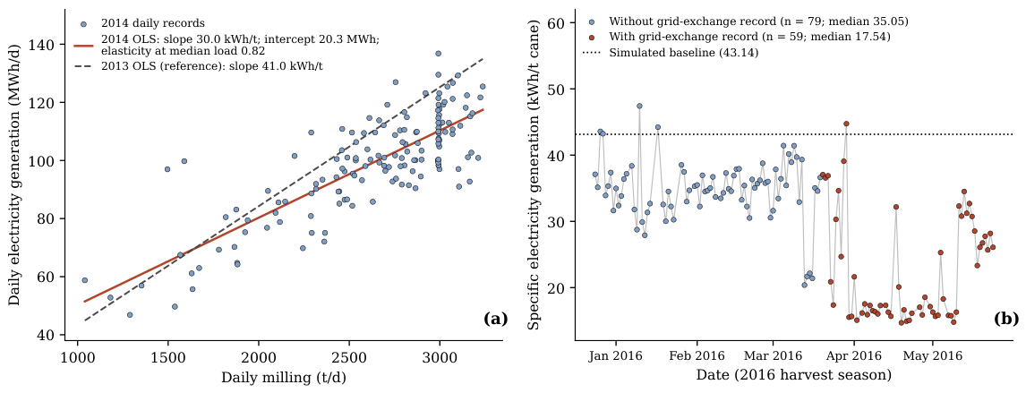
The markedly lower median specific generation of the descriptive 2016 season (32.35 kWh/t; CV 29.6%) warrants a dedicated diagnostic, as shown in Figure A3b (Appendix A). The grid-exchange records of 2016 are not missing at random: they exist exclusively for the final 59 operating days of the season (20 March to 24 May 2016), whereas the first 79 days (December–March) lack them entirely. The two subsets differ sharply in independently metered generation: median of 17.54 kWh/t on the days with grid records versus 35.05 kWh/t on the days without them (two-sided Mann–Whitney, ), with the monthly medians collapsing from 33–36 kWh/t in December–March to 16.44 kWh/t in April. Two conclusions follow. First, the low 2016 generation is genuine late-season operational deterioration, not a metering artifact: specific generation is metered independently of the grid-exchange records. Second, the recorded export series is not merely incomplete but systematically biased toward the degraded tail of the season, which converts the exclusion of 2016 from gap estimation (Section 2.3) from a discretionary choice into a necessity; its recorded median export of 0.33 kWh/t is unrepresentative by construction. The sensitivity of the pooled estimates is nevertheless quantified: including 2016 moves the generation-level discount factor from 0.89 to 0.87 (pooled median of 38.18 to 37.51 kWh/t), while the export-level factor cannot include 2016 at all because its export series is the biased subset just described.
The figure reveals the central finding of this study: no harvest median reaches the simulated base case (43.14 kWh/t), and the daily dispersion is wide, with boxes that expand notably in the 2013 and 2015 harvests. Real operation is not located at a stable point close to the design value but, rather, in a cloud of systematically lower values; the assumption of continuous nominal operation underlying simulation-based studies is not satisfied in any of the seven harvests.
3.2. Magnitude of the Gap in the Main Sugar Mill
The gap is quantified at three levels. At Level 1 (specific electricity generation), it ranges from 5.9 to 15.2% relative to the base case depending on the harvest (multiharvest pooled median of 37.51 vs. 43.14 kWh/t when the descriptive 2016 season is included; 38.18 kWh/t for 2010–2015). At Level 3 (absolute harvest energy), which integrates availability, milling rate, and export intensity, it ranges from 19.0 to 49.3% (median 41.5%): for the 2010–2015 period, the mill exported 20,885 MWh against a simulated potential of 33,720 MWh, corresponding to an aggregated gap of 38.1%, equivalent to 12,835 MWh not realized over six harvests, increasing to 47.9% relative to the improved case. Level 2 (specific export to the SEN) is represented in Figure 2, which shows the daily distribution of export by harvest against the two simulation anchors.
Figure 2.
Daily distribution of specific grid export to the SEN by harvest against the simulated anchors.
The distribution confirms and amplifies the pattern observed in generation: median daily export ranges from 8.7 to 12.8 kWh/t depending on the harvest, always below the base case (14.13 kWh/t) and far below the improved case (16.81 kWh/t), with an export gap ranging from 9.3 to 38.4% relative to the base case. Only the 2013 harvest approaches the base-case anchor, and none exceeds it. Table 3 details the Level-3 gap and its multiplicative decomposition by harvest, which is analyzed in Section 3.4.
Table 3.
Level-3 energy performance gap and multiplicative decomposition (2010–2015 harvests).
3.3. The Gap at Provincial Scale
To verify whether the underperformance is idiosyncratic to the 14 de Julio mill or part of a broader pattern, the simulated performance of the five mills in the province is compared against their aggregated real operation. Figure 3 shows the simulated export of each mill, the milling-weighted provincial simulated average, and the aggregated real provincial export.
Figure 3.
Simulated electricity export (base case) of the five mills in the province, the milling-weighted provincial simulated mean, and the aggregate real provincial export (2013/14–2015/16 harvests). The provincial gap is 28.9%.
Simulated export by mill varies widely (6.01–14.13 kWh/t). This heterogeneity is structural: the five schemes differ in installed turbogenerator capacity relative to milling rate, in process-steam demand, and in available bagasse per unit of throughput (Table 4); in particular, the two largest mills by milling capacity (Antonio Sánchez and 5 de Septiembre) exhibit the lowest simulated export intensities, so the milling-weighted provincial average (10.13 kWh/t) lies well below the best individual scheme. Compared with an aggregated real export of 7.20 kWh/t over the 2013/14–2015/16 harvests, the provincial gap is 28.9% (37.5% relative to the improved case). As a robustness check, extending the real aggregate to the five available seasons (2011/12–2015/16) yields 7.40 kWh/t and a gap of 27.0%, confirming that the result is not driven by the choice of period. This result is decisive for the scope of the study: underperformance is also observed at the aggregate level of the five mills, with a magnitude of the same order as in the individual case, indicating that it is not a peculiarity of the main mill. However, a clarification is required, as detailed in Table 4: only the main mill has individual operational records; therefore, this result represents an aggregated provincial gap, not five individually validated gaps.
Table 4.
Simulation of the five mills (base case) and aggregated real provincial performance.
The structural heterogeneity of the simulated intensities (6.01–14.13 kWh/t) raises the question of whether the aggregate discount is uniform across configurations or concentrated in specific schemes. Subgroup-specific gaps cannot be computed directly because real export exists only as a provincial aggregate; two bounding analyses nevertheless constrain the answer. First, decomposing the aggregate into the measured mill and the four unmeasured mills, with the milling weight of 14 de Julio (17.7%) and its measured intensity ODF of 0.71 [0.68; 0.75], the joint discount factor implied for the remaining four schemes is 0.711 [0.698; 0.720]—numerically indistinguishable from the measured mill. Second, splitting the fleet into high-intensity (>10 kWh/t: 14 de Julio, Ciudad Caracas, Elpidio Gómez; milling-weighted simulated export 13.08 kWh/t; 51.4% of provincial milling) and low-intensity schemes (<10 kWh/t: Antonio Sánchez, 5 de Septiembre; 7.01 kWh/t; 48.6%), if the low-intensity subgroup operated with no gap, the high-intensity subgroup would require an ODF of 0.56, whereas confining the entire gap to the low-intensity subgroup would require an ODF of 0.14 for it—a value incompatible with the 0.71 measured at a high-intensity mill and physically implausible. Within the resolution the aggregated data permit, the underperformance is therefore consistent with a uniform discount across the fleet rather than with concentration in a single configuration class; individual metering of the remaining mills, identified as future work, is required to resolve it further. This consistency analysis assumes comparable availability and milling utilization across mills and is reported as a bound, not as validation.
3.4. The Gap Is in Generation, Not in Idle Capacity
The first step in locating the origin of the gap is to decompose the energy ratio () into its three multiplicative factors. Figure 4 presents, by harvest, availability (), milling utilization (), and export intensity (), together with their product.
Figure 4.
Multiplicative decomposition of the ratio by harvest: availability (), milling utilization (), and export intensity ().
The figure immediately rules out two potential drivers: availability is nearly unitary across all harvests, and milling utilization introduces only a moderate and stable reduction (–). The dominant and, more importantly, most variable factor is export intensity (–), which explains most of the gap and its entire interannual variability: the harvest of 2013, which shows the smallest gap, is characterized exclusively by its intensity (0.929), not by more operating days or higher milling rates.
The origin of the gap is therefore located in export intensity, which is further decomposed additively per tonne of cane in Figure 5, using cane-weighted means over the 792 days of 2010–2015 with complete grid-exchange records (Section 2.5).
Figure 5.
Additive decomposition of the specific export gap (cane-weighted means, 792 days with complete grid-exchange records, 2010–2015 harvests): from the simulated base-case export to the observed real export. The decomposition closes exactly because industrial consumption is the metered residual of the daily balance.
The additive decomposition yields a counterintuitive result. Real industrial electricity demand (29.18 kWh/t, cane-weighted mean) is almost identical to the simulated demand (29.01 kWh/t; deviation kWh/t or %): the factory does not consume meaningfully more than expected, so demand does not explain the gap. The deficit lies in generation (37.68 vs. 43.14 kWh/t; kWh/t, %), partially offset by grid imports (1.43 kWh/t), reproducing the observed export of 9.93 kWh/t with exact closure (100.0%); the resulting total export gap is kWh/t, i.e., % of the simulated baseline export.
A statistical control confirms the interpretation. Table 5 reports the intra-harvest correlation between specific generation and milling load, harvest by harvest, along with sample sizes, p-values, and confidence intervals. In no harvest does specific generation increase significantly with load, except 2010, where the association is weak (); in 2014, the association is significantly negative (). The mean intra-harvest correlation is . Underutilization of capacity therefore fails to explain the deficit, and the negative 2014 association reinforces the conclusion: the gap is one of conversion efficiency, not idle capacity.
Table 5.
Intra-harvest Pearson correlation between daily specific generation and milling load.
The significantly negative 2014 association () is mechanically counterintuitive for a back-pressure system and is therefore examined in Figure A3a (Appendix A). Three candidate explanations are tested. Progressive equipment degradation is not supported: the correlation is stable across the two halves of the season ( and ), and specific generation on low-milling days remains at normal levels (median of 38.91 kWh/t below the median load versus 36.55 kWh/t above it). Measurement drift is not supported either: absolute daily generation correlates strongly and positively with milling (), and the daily balance closes by construction. What distinguishes 2014 is the shape of the generation–throughput relationship: the marginal generation is 30.0 kWh per additional tonne—against 35.9–41.0 kWh/t in the other five harvests—with a positive intercept of 20.3 MWh/day (against to MWh in the other harvests), yielding an elasticity of 0.82 at the median load. Generation therefore grew sub-proportionally with throughput: at high milling rates, part of the incremental steam was routed to process demand or losses rather than through the turbogenerators, which mechanically produces the negative correlation between the specific indicator and load. This is consistent with a steam-side constraint concurrent with process-steam demand rather than with degradation or metering drift, although the accounting nature of the steam records precludes direct verification. The influence of 2014 on the pooled synthesis is bounded: excluding it moves the export-level discount factor from 0.712 to 0.718, so the pooled gap is not driven by this harvest.
3.5. The Start-of-Season Regime with Pressure-Reducing Valves in Service
Having established that the deficit arises from conversion efficiency, the plant steam records were examined for operational information. As declared in Section 2.3, the recorded steam magnitudes are accounting allocations built from fixed coefficients; any correlation between an allocation-based bypass fraction and specific generation is arithmetic by construction—on the subset of days with a non-zero reducer allocation, that correlation equals exactly—and is therefore not reported as evidence. The records do, however, contain one operationally independent variable: the binary indicator of whether the pressure-reducing valves were in service. Its independence from the electricity series is demonstrable: 90 of the 138 recorded days have specific generation below the accounting break-even of 41.08 kWh/t and would necessarily carry a positive reducer allocation under the fixed coefficients yet are recorded with the reducers closed, and the generation ranges of the two groups overlap (up to 36.76 kWh/t among reducer days; down to 31.41 kWh/t among closed days).
The structure of this indicator is, itself, informative: the reducers were in service during a single contiguous block of 39 days at the start of the 2015 harvest (2 December 2014 to 9 January 2015; 28.3% of the operating days), with exactly one state change over the whole season. Figure 6 presents this evidence in two complementary views: Figure 6a shows the daily specific generation across the season with the regime highlighted, and Figure 6b contrasts the distributions of daily generation under the two regimes.
Figure 6.
The start-of-season regime with pressure-reducing valves in service (2015 harvest). (a) Daily specific electricity generation across the season; the shaded band marks the contiguous 39-day regime with the reducers in service, dashed lines mark the median of each regime, and the dotted line represents the simulated baseline. (b) Distribution of daily specific generation by regime (boxes: quartiles; line: median; points: individual days), with the one-sided Mann–Whitney significance and Cliff’s effect size.
The contrast between regimes is large and statistically unambiguous: median specific generation was 26.15 kWh/t with the reducers in service versus 38.06 kWh/t with the reducers closed, a difference of 11.9 kWh/t (one-sided Mann–Whitney U, ; point-biserial ; Cliff’s —a very large effect). Crucially, the milling rate is statistically indistinguishable between regimes (medians of 2994 vs. 2992 t/d; two-sided Mann–Whitney, ), so the regime deficit is not a load effect. Expressed in the plant’s own accounting convention (12.17 kg of steam per kWh), the regime deficit corresponds to diverting on the order of one-tenth of the season’s steam away from the turbogenerators, which is the accounting translation—not an independent measurement—of the same electricity deficit.
Two interpretive boundaries must be stated. First, this evidence comes from a single harvest with daily steam records, and its generality is unknown. Second, the regime contrast identifies a start-of-season operating configuration, not an isolated mechanism: reducers in service plausibly coincide with other start-up factors (equipment warm-up, boiler tuning, early-season bagasse moisture, and maintenance state), and the available data cannot apportion the deficit among them. What the finding does establish, within these boundaries, is that the conversion deficit is concentrated in an identifiable, calendar-bounded operating regime whose shortening or tightening is an operational decision requiring no capital investment—the same class of measure that the improved simulated case represents by reducing the reducer flow to 0.1% (Table 1).
Whether this start-of-season configuration is recurrent or anomalous cannot be tested directly because the reducer-state indicator exists only in the 2015 steam records; it can, however, be tested indirectly on the metered electricity series of all seasons through the start-of-season contrast defined in Section 2.9, as shown in Figure A1 (Appendix A). Over the first 20 operating days, a significant depression of median specific generation appears in four of the six estimable harvests: kWh/t in 2010 (Cliff’s ; ), kWh/t in 2011 (; ), kWh/t in 2012 (; ), and kWh/t in 2015 (; ), with no depression in 2013 or 2014 and a mean effect size of across 2010–2015. Two qualifications bound this evidence. First, load confounding is heterogeneous: milling rates in the opening window are statistically indistinguishable from the rest of the season in 2011 () and 2015 ()—the cleanest cases—but significantly lower in 2010 and 2012, where part of the early deficit could reflect load, although the weak or negative within-harvest generation–load correlations of Table 5 limit that channel. Second, in the full 39-day window of the documented regime, only 2015 sustains a large effect ( kWh/t; ), with a mild residual effect in 2011 ( kWh/t; ). The reading that the data support is therefore twofold: a moderate start-of-season depression of 3–4.5 kWh/t over roughly the first three weeks is a recurrent feature of this plant, and the 2015 reducer regime is its most severe and most prolonged documented instance—exceptional in depth and duration but not an isolated anomaly in kind. This places the single-harvest regime evidence within an inter-harvest pattern without overstating its generality.
3.6. Consistency of the Bagasse Accounting
The 2015 bagasse sheet records a median bagasse surplus of 14.1% of produced bagasse, compared to 28.25% in the simulated base case and 33.95% in the improved case. Because the bagasse allocations in the plant records are derived from the electricity series through the same fixed coefficients as the steam allocations (Section 2.3), this figure is the mass-side accounting translation of the observed generation deficit—a less efficient bagasse-to-electricity conversion consumes a larger recorded fraction of the available bagasse while delivering lower output—and it is reported here strictly as an internal-consistency check of the plant’s own bookkeeping, not as independent validation of the electrical balance.
3.7. Temporal Stability of the Gap
The Mann–Kendall test applied to the interannual medians of specific generation (2010–2016) does not detect a significant monotonic trend (; ; ). The statistical power of this test at is, however, limited: Monte Carlo simulation with the empirical interannual standard deviation (2.53 kWh/t) shows that only trends steeper than approximately 2.25 kWh/t per harvest—equivalent to a cumulative drift of about 36% of the mean level over the period—would be detected with 80% power. The null result is therefore consistent with, though not conclusive proof of, a structurally stable gap: within the detectability limits of the series, the system operates in a state systematically below the simulated benchmark without evidence of progressive deterioration, suggesting that the gap will not close spontaneously and requires deliberate operational intervention.
3.8. Operational Discount Factor
As a case-specific quantitative synthesis of the gap, Figure 7 presents the operational discount factors with their block-bootstrap confidence intervals. For electricity export intensity, the factor relative to the base case is 0.71 (95% CI [0.68; 0.75]) and 0.60 ([0.57; 0.63]) relative to the improved case; for specific generation, it is 0.89 ([0.87; 0.90]). The point estimates are invariant to the bootstrap block length (5, 10, and 20 days), and the confidence-interval half-widths increase only moderately with longer blocks (0.031, 0.037, and 0.048, respectively, for export intensity), supporting the robustness of the interval estimates to this methodological choice.
Figure 7.
Operational discount factors (real/simulated) with 95% block-bootstrap confidence intervals (10-day blocks): export intensity against the baseline and improved cases, specific generation against the baseline, and the derived seasonal-energy factor (). The dotted line indicates no gap (ODF = 1).
Because investment decisions concern total seasonal energy, the energy-level factor is reported separately: the directly observed ratio is for 2010–2015, consistent with the composition of Equation (4). The distinction matters in application: multiplying a simulated seasonal energy potential by the intensity factor alone (0.71) would under-correct it because sub-nominal milling and availability losses would be omitted. For systems of this class, simulated export potentials should be corrected with the factor matching the decision variable—0.71 for specific intensity and 0.62 for seasonal energy—or, alternatively, the baseline simulation should be calibrated against operational data; in either case, these numerical values are specific to this plant and period, and their transfer to other configurations requires replication.
3.9. Parametric Uncertainty of the Baseline and Total Uncertainty of the Discount Factor
Figure A2 (Appendix A) presents the Monte Carlo characterization of the simulated baseline defined in Section 2.9. Under normal perturbations ( at the reviewer-specified limits), the 95% interval of the baseline export intensity is kWh/t (median of 14.11, reproducing the nominal 14.13), and under worst-case uniform perturbations, it is kWh/t. The subtraction of the industrial demand amplifies the –8% parametric uncertainty at the generation level into a % uncertainty at the export level, so the half-width of the baseline interval spans on the order of 80–90% of the observed intensity gap of 4.07 kWh/t. Three consequences follow, and all three must be stated. First, the existence and sign of the gap are robust to parametric model uncertainty: the probability that the observed pooled median export reaches or exceeds the perturbed baseline is 0.7% under normal and 1.1% under worst-case uniform perturbations at the export level and, at most, 0.1% at the generation level, where the amplification is absent. Second, the magnitude of the intensity-level discount factor is materially model-dependent: propagating the parametric uncertainty yields an ODF interval of [0.57; 0.93], and combining it with the block-bootstrap sampling uncertainty leaves the total 95% interval essentially unchanged, at [0.57; 0.93], dominated by the parametric component. The point estimate of 0.71 [0.68; 0.75] must therefore be read as conditional on the nominal parameterization of STA 4.1, with the wider band expressing total uncertainty. Third, three observations external to the simulator constrain how much of the gap the parametric channel can plausibly absorb: the measured industrial demand matches the simulated value to %, the specific steam rate embedded in the plant records (12.17 kg/kWh) matches the thermodynamic expectation for the installed configuration (Section 2.2), and the regime contrast of Section 3.5 (11.9 kWh/t at identical milling rates) is entirely model-free. The seasonal-energy factor of 0.62 is likewise partially insulated because its availability and milling-utilization components ( and ) are measured, not simulated.
Instrument uncertainty adds a second, smaller component. Because the discount factor is median-based, independent day-level metering noise averages out over the 792 pooled days, and the combined Monte Carlo (sampling × Class-1.0 calibration bias) widens the interval by less than 0.005; the worst-case deterministic bounds under a systematic calibration bias are [0.677; 0.754] for Class 0.5 m and [0.673; 0.758] for Class 1.0. The statement in Section 2.8 that the bootstrap intervals exclude these components is thereby replaced by an explicit quantification: sampling and instrument components are of the order of hundredths, while the parametric-model component is of the order of tenths and dominates the error budget of the intensity-level factor.
4. Discussion
4.1. Magnitude of the Gap in Relation to the Performance Gap Literature
The quantified gap—19 to 49% per harvest, 38.1% aggregated at the mill level, and 28.9% at the provincial level—falls squarely within the range documented for the energy performance gap (EPG) in buildings. The reported mean deviation of with a standard deviation of 55% across 62 buildings [30] and the prediction-to-measurement ratio ranging from 0.38 to 4 [31] position these results as one instance of a cross-cutting phenomenon across energy systems rather than an anomaly specific to the sugar industry.
Moreover, de Wilde’s framework highlights that the magnitude of the gap depends on the temporal resolution at which it is assessed [29]; the daily-resolution design of this study, compared with the seasonal averages typically used in the sugar sector, is precisely what allows the variability to be observed (coefficient of variation ranging from 9.9 to 29.6%), which would otherwise be masked by aggregation.
The contribution is therefore not the observation that real systems underperform simulations—an intuition familiar to operators and qualitatively acknowledged in the sector as recurrent project failures [27]—but the quantification, decomposition, and regime-level localization of the gap using daily operational data in a field where the literature has been dominated by simulation-based approaches [4,10], together with an explicit audit of which recorded plant variables can—and which cannot—support empirical inference.
4.2. A Causal Reading: From the Building Performance Framework to the Sugar Mill
The diagnostic value of the results becomes evident when mapped onto the causal categories identified in the building performance gap literature [30]. The first source, model specification uncertainty, corresponds to the deterministic nature of STA 4.1, which simulates nominal steady-state operation without incorporating operational variability; its effect is manifested in the fact that the base case, rather than acting as a lower bound, becomes an upper benchmark that real operation never reaches, and its magnitude is now bounded quantitatively by the stochastic surrogate of Section 2.9 and Section 3.9. The second source, occupant behavior—whose weight in buildings is subject to active debate and even concerns of over-attribution [32,33,34]—has no direct analog in a plant without occupants, and its absence helps explain why the observed gap is more structural and less stochastic than that typically found in office buildings, consistent with the absence of a detectable interannual trend (Section 3.7). The third source, operational practices—to which the review attributes up to 80% of the gap—is illuminated here not by a correlation, which the accounting nature of the steam records precludes, but by regime evidence: a calendar-bounded start-of-season configuration with pressure-reducing valves in service during which conversion was 11.9 kWh/t lower at identical milling rates, now placed within a recurrent inter-harvest start-of-season pattern (Section 3.5). In buildings, the established method to disentangle and quantify these causes is model calibration against measured data [35,36]; this work provides the sectoral analog of the confrontation step, and the building framework, by excluding non-applicable causes, focuses attention on the operational-practice category to which the identified regime belongs.
4.3. Why the Margin Lies in Steam Management and Not in Turbine Efficiency
A methodological clarification is necessary for interpretability. The specific steam consumption embedded in the plant records (12.17 kg/kWh) could be hastily read as evidence of inefficient turbogenerators; thermodynamic analysis contradicts this: it is the expected value for a back-pressure turbine operating at 17–23 bar with process-steam exhaust, compared with the approximately 5–6 kg/kWh typical of high-pressure systems [9,38]. The sector literature further confirms that low-efficiency configurations typically operate with live steam at around 22 bar and 300 °C [18] and that the main gains in surplus electricity arise from increasing pressure levels and the shift toward CEST configurations [3,4]. Attributing the gap to turbine inefficiency would therefore constitute a diagnostic error: the limitations of low-pressure systems belong to capital-intensive modernization of the steam cycle, not to operational deficiencies of existing equipment. The margin that is reducible without investment lies in steam management, and the regime evidence of Section 3.5 locates it concretely in the start-of-season configuration with reducers in service. Thus, the diagnostic separates two distinct horizons: short-term steam management without capital investment and long-term pressure-level upgrading requiring capital deployment.
A further layer of the same diagnostic concerns the feedstock itself. The simulation treats bagasse as a uniform energy carrier, yet the lignocellulosic matrix delivered at the start of the season differs systematically from mid-season material: early-cut cane and rain-season harvesting raise bagasse moisture and extraneous matter, depressing the lower heating value—approximately 208 kJ/kg per percentage point of moisture [47]—and boiler combustion stability. Under such conditions, sustaining live-steam pressure for the turbogenerators becomes harder precisely when process-steam demand must still be met, and routing steam through the pressure-reducing valves is the operationally conservative response; degraded early-season biomass quality is therefore not merely a co-occurring factor but a plausible driver of the very bypass regime documented in Section 3.5, and it may also contribute to the recurrent moderate start-of-season depression of Figure A1. The available records contain no physicochemical characterization of the bagasse, so this mechanism cannot be tested retrospectively; what can be specified is the monitoring protocol that would make it testable in future campaigns: daily composite bagasse sampling at the boiler feeders during at least the first six weeks of the season and weekly thereafter, with determination of moisture (oven drying), ash, and higher/lower heating value (bomb calorimetry), complemented by a basic compositional profile (fiber and Brix of residual juice) at weekly resolution, all logged against the reducer-state indicator and the metered electricity series. Together with direct steam-flow measurement on the turbogenerator and bypass lines—for which non-invasive clamp-on ultrasonic flow meters on the main steam headers are the natural retrofit, enabling thermodynamic validation of the specific steam consumption baseline without piping modifications—this would convert the accounting-based steam records into an instrumented dataset capable of apportioning the start-of-season deficit among feedstock quality, equipment warm-up, and steam-management practice.
4.4. The Discount Factor and the Absence of a Measurement and Verification Framework
The main practical deliverable is the operational discount factor in its two forms. The fact that the simulated export potential must be discounted by approximately 30% in intensity terms (ODF ≈ 0.71) and by approximately 40% in seasonal-energy terms (0.62) before being used to support investment decisions is a correction that is currently absent in sugar-energy planning, whereas in buildings, it is standardized through a comprehensive measurement and verification (M&V) framework. The International Performance Measurement and Verification Protocol (IPMVP) defines its Option D—calibrated simulation—precisely to anchor a model to measured data and recommends using the first year of stable operation as a new baseline against which improvements are assessed [49], which is effectively the operational translation of calibrating the baseline case against measured performance.
ASHRAE Guideline 14 introduces statistical thresholds for bias and fractional uncertainty in savings, which govern the temporal granularity of the model [50], while ISO 50001 and ISO 50015 institutionalize the concept of energy baselines and performance indicators, as well as the verification of improvements at the organizational level [51,52]. The proposed ODF can be interpreted as an energy performance indicator—in the sense of these standards—that translates the simulation–operation gap into a single, auditable coefficient, provided the intensity and energy levels are not conflated.
Moreover, the issue extends beyond buildings: in wind and solar power generation, overestimating or underestimating production has direct financial consequences—such as debt-covenant breaches or missed investment opportunities—and is managed using correlation techniques with reference periods, where the main risk is, again, the representativeness of the selected period [53]. The factors derived here are a minimal version of the same concept applied to sugarcane cogeneration: specific to this class of system and time period—therefore, their numerical values should not be extrapolated without replication—but based on a fully transferable and, with the deposited data and scripts, fully reproducible procedure.
A final qualification bounds the transferability of the factors by technology class. The derived ODFs are tightly bound to the thermodynamic limits of a low-pressure back-pressure configuration, in which electricity is a by-product rigidly coupled to process-steam demand: generation cannot exceed what the process pulls through the turbines, so operational shortfalls translate almost entirely into lost export, and the export level amplifies generation-level deviations because the (accurately predicted) internal demand is subtracted from a diminished generation. A mill equipped with an extraction–condensing steam turbine (CEST) faces a structurally different gap: the condensing path decouples generation from process demand, giving the operator a degree of freedom to sustain output during process fluctuations while introducing failure modes absent here (condenser vacuum and cooling-water limitations) and a stronger sensitivity to fuel availability, since surplus power competes directly for bagasse. A CEST plant would therefore be expected to exhibit a different—plausibly smaller and differently structured—energy performance gap, and its discount factor would require independent calibration on its own operational records; the numerical values derived here apply to the low-pressure BPST class only, while the derivation procedure applies to both.
4.5. Implications for Undercapitalized Sugar Mills
For low-pressure sugar mills with restricted access to capital—as in the Cuban case and in segments of Sub-Saharan Africa, South Asia, and Southeast Asia, where bagasse-based cogeneration is both mature and underexploited [1,2,3]—the priority order suggested by the results is as follows: first, close the operational gap without capital investment by tightening the start-of-season regime with pressure-reducing valves in service and bringing milling operation closer to installed capacity, whose upper bound is given by the simulated base case (approximately % export relative to the observed pooled median), and only thereafter consider capital-intensive retrofits (high-pressure systems, CEST), whose financial assessment must be based on baselines corrected with the operational discount factor appropriate to the decision variable.
The gap admits a direct monetary translation under the purchase-tariff framework in force during the study period (Resolution 425/2011 of the Ministry of Finance and Prices, which set time-of-day tariffs for biofuel-based cogeneration with a fuel-price adjustment coefficient [48]) and the AZCUBA planning prices applied in the economic module of STA 4.1 (0.16 CUP/kWh sold; 0.20 CUP/kWh purchased; official enterprise exchange rate of 1 CUP = 1 USD in the period). The 12,835 MWh of unrealized export over 2010–2015 represents approximately 2.05 million CUP of foregone revenue—on the order of 0.34 million CUP per harvest—to which the 3008 MWh of grid imports add 0.60 million CUP of direct expenditure. Per unit of throughput, the export gap of 4.20 kWh/t and the imports of 1.43 kWh/t translate into a financial leakage of 0.96 CUP per tonne of cane, equivalent to about 1.0% of the cane price itself (95 CUP/t); the 39-day reducer regime of 2015 alone accounts for roughly 1389 MWh and 0.22 million CUP for a single start of season. For an undercapitalized mill, these are not marginal figures: they are recurrent losses of the same order as the entire annual electricity revenue line of the plant, recoverable in large part through the no-capital steam-management measures identified above.
Investing capital on inflated baselines leads to systematically overestimated expected returns, precisely in contexts with the least capacity to absorb such errors; the reverse order—operational optimization first, capital investment second—protects the economic viability of the transition and constitutes, in itself, a low-cost decarbonization measure, since every megawatt-hour recovered from the existing bagasse displaces fossil generation on the national grid.
4.6. Limitations
First, individual operational records are available for a single mill; the provincial result is an aggregated gap over five mills, not five individually validated gaps, and sector-wide generalization requires replication with measured data from other schemes. Second, the study period (2010–2016) predates the recent downturn of the Cuban agro-industrial sector; the analysis is a retrospective methodological assessment rather than a diagnosis of the current state of the system. Third, STA 4.1 is deterministic; its parametric uncertainty is now bounded through the first-order stochastic surrogate of Section 2.9 and Section 3.9, which quantifies but does not eliminate the conflation of model-specification error and operational deviation, and benchmarking STA 4.1 against an independent simulation platform remains a natural extension. Fourth, the steam and bagasse magnitudes in the plant records are accounting allocations built from fixed coefficients; only the binary indicator of the pressure reducers being in service is operationally independent, and the regime contrast built on it cannot apportion the observed deficit among the co-occurring start-of-season factors (equipment warm-up, boiler tuning, early-season bagasse moisture, fouling, steam leaks, maintenance practices, or instrument calibration), none of which is measured in the available records. Fifth, the regime evidence rests on a single harvest (2015) with daily steam records, although the indirect start-of-season contrast of Section 3.5 now places it within a recurrent inter-harvest pattern. Sixth, the 2016 harvest was excluded because 57% of its operating days lack grid-exchange records, a gap shown in Section 3.1 to be systematically concentrated in the degraded final stretch of the season. Seventh, the block-bootstrap intervals reflect sampling variability under serial dependence only; the parametric-model and instrument components are now quantified separately in Section 3.9, where the parametric component is shown to dominate the total error budget of the intensity-level factor ([0.57; 0.93]), while the surrogate used for that quantification is, itself, a first-order multiplicative approximation of the STA 4.1 balance, not a replacement for benchmarking against an independent platform. Eighth, the start-of-season contrast of Section 3.5 is partially confounded by lower early-season milling in the 2010 and 2012 harvests, and the economic valuation of Section 4.5 relies on administered planning prices rather than market prices, so it measures foregone revenue under the prevailing tariff framework, not economic value in a market sense.
5. Conclusions
This study quantifies, from a seven-harvest daily operational dataset of a low-pressure sugar mill, the gap between the electricity surplus predicted by simulation and the electricity actually delivered to the grid —a discrepancy repeatedly acknowledged in the sector literature but not previously confronted with multiyear daily records—and frames it within the energy performance gap (EPG) concept.
The absolute export gap relative to the simulated base case ranges from 19.0 to 49.3% depending on the harvest (38.1% aggregated over 2010–2015; 12,835 MWh unrealized), and at the level of the five-mill provincial aggregate, it reaches 28.9% (27.0% when extended to the five available seasons), indicating that the underperformance is not idiosyncratic to the case-study mill.
The gap does not arise from idle capacity: availability is nearly complete (98–100%), the cane-weighted real demand matches the simulated demand (29.18 vs. 29.01 kWh/t), and in no harvest does specific generation increase significantly with milling load; the deficit is located in conversion (5.46 kWh/t; %), with the additive decomposition closing exactly.
The plant steam records proved to be accounting allocations and cannot support correlation-based inference; their single operationally independent variable documents a contiguous start-of-season regime with pressure-reducing valves in service (39 days of the 2015 harvest) during which specific generation was 11.9 kWh/t lower at statistically identical milling rates (26.15 vs. 38.06 kWh/t; ; Cliff’s ). Thus, within the limits of single-harvest evidence, the conversion deficit is concentrated in an identifiable, calendar-bounded operating configuration whose tightening requires no capital investment; the data cannot apportion the deficit among the mechanisms that co-occur in that configuration.
No interannual trend was detected (Mann–Kendall, ); given the limited power of the test at (minimum detectable trend of approximately 2.25 kWh/t per harvest), this result is consistent with, though not conclusive proof of, a persistent structural gap.
The parametric uncertainty of the deterministic baseline is characterized through a calibrated stochastic surrogate: the existence of the gap survives worst-case perturbations of the simulation inputs (probability of no gap of, at most, 1.1% at the export level and 0.1% at the generation level), while the intensity-level discount factor carries a total 95% interval of [0.57; 0.93], dominated by the model-parametric component, so its point value of 0.71 is conditional on the nominal parameterization. A start-of-season depression of 3–4.5 kWh/t over the first three operating weeks recurs in four of six estimable harvests, identifying the 2015 reducer regime as the most severe instance of a recurrent pattern rather than an isolated anomaly; and the gap translates into a financial leakage of approximately 0.96 CUP per tonne of cane under the tariff framework of the period.
Case-specific operational discount factors are derived with block-bootstrap confidence intervals: 0.71 ([0.68; 0.75]) for export intensity and 0.62 for total seasonal energy, with the latter composing intensity with availability and milling utilization. The transferable output is the derivation and correction procedure; the numerical values are specific to this plant and period and must be replicated before use elsewhere.
Future work is directed along four main lines: consolidating the separation of model error from operational variability initiated here by benchmarking the stochastic surrogate of the STA model against an independent simulation platform; replicating the framework with measured data from other mills to replace the aggregated provincial gap with individual mill-level gaps and to test the transferability of the discount factors; extending the steam records—ideally with direct flow measurement—across additional harvests to test the generality of the start-of-season reducer regime; and instrumenting the candidate start-up factors through the combined protocol specified in Section 4.3—daily physicochemical bagasse sampling (moisture, ash, calorific value, and basic compositional profile) during the opening weeks of the season, together with non-invasive ultrasonic steam-flow measurement on the turbogenerator and bypass headers—so that the regime deficit can be apportioned among feedstock quality, equipment warm-up, and steam-management practice and the specific steam consumption baseline can be validated thermodynamically.
Author Contributions
Conceptualization, R.J.B. and Y.C.A.; methodology, R.J.B., Y.C.A. and J.R.R.; software, R.J.B., Y.C.A., L.A.I.C. and A.L.L.; validation, R.J.B., Y.C.A., P.Y.S.-C., J.B.R.-O., L.A.I.C. and J.R.R.; formal analysis, R.J.B., Y.C.A., P.Y.S.-C., A.L.L. and J.R.R.; investigation, R.J.B., Y.C.A., J.B.R.-O. and A.L.L.; resources, R.J.B. and Y.C.A.; data curation, R.J.B., Y.C.A., L.A.I.C. and A.L.L.; writing—original draft preparation, R.J.B. and Y.C.A.; writing—review and editing, R.J.B., Y.C.A., P.Y.S.-C., J.B.R.-O., L.A.I.C., A.L.L. and J.R.R.; visualization, R.J.B., Y.C.A., P.Y.S.-C. and J.B.R.-O.; supervision, R.J.B., Y.C.A. and J.R.R.; project administration, R.J.B. and Y.C.A. All authors have read and agreed to the published version of the manuscript.
Funding
This research received no external funding.
Data Availability Statement
The original contributions presented in this study are included in the article. Further inquiries may be directed to the corresponding authors.
Acknowledgments
The authors thank the operational staff of the “14 de Julio” sugar mill for the harvest records that made this analysis possible. During the preparation of this manuscript, the authors used Grammarly v 2026 to review the grammar of the full manuscript. The authors have reviewed and edited the output and take full responsibility for the content of this publication.
Conflicts of Interest
The authors declare no conflicts of interest.
Abbreviations
The following abbreviations are used in this manuscript:
| BIGCC | Biomass Integrated Gasification Combined Cycle |
| BPST | Back-pressure Steam Turbine |
| CEST | Condensing–Extraction Steam Turbine |
| CV | Coefficient of Variation |
| EPG | Energy Performance Gap |
| LHV | Lower Heating Value |
| ODF | Operational Discount Factor |
| IG | Specific Electricity Generation (kWh per t of cane) |
| SEN | Sistema Electroenergético Nacional (Cuban national grid) |
| STA | Sistema Termoazúcar (sugar-mill thermal balance simulator) |
Appendix A
Table A1.
Thermodynamic parameters and constraints defining the STA 4.1 baseline case of the 14 de Julio sugar mill (from [24,26] and the underlying field audit).
Figure A1.
Start-of-season contrast in median specific generation for (a) the first and (b) the first operating days versus the rest of each season. Red bars: significant one-sided Mann–Whitney depression (* ; *** ), with Cliff’s annotated; gray: 2016, descriptive only.
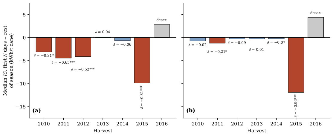
Figure A2.
Monte Carlo characterization of the simulated baseline (normal perturbations, at the limits: boiler efficiency %, isentropic efficiency %, bagasse moisture points; draws). (a) Distribution of the baseline export intensity () against the nominal value and the observed pooled median. (b) Resulting distribution of the export-intensity discount factor under parametric uncertainty.
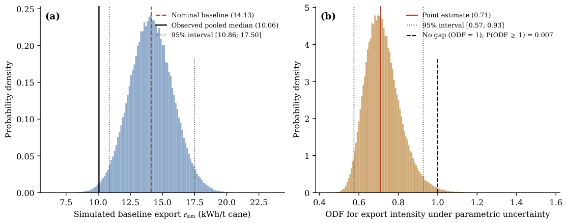
Figure A3.
Diagnostics for the two atypical harvests. (a) 2014: daily generation versus milling, with the 2014 OLS fit (marginal generation of 30.0 kWh per additional tonne; positive intercept) against the 2013 reference; the sub-proportional scaling mechanically produces the negative correlation between specific generation and load. (b) 2016: daily specific generation colored by availability of the grid-exchange record; records exist only for the degraded final 59 days of the season, so the recorded export series is systematically biased, not merely incomplete.
References
- Khatiwada, D.; Seabra, J.; Silveira, S.; Walter, A. Power generation from sugarcane biomass—A complementary option to hydroelectricity in Nepal and Brazil. Energy 2012, 48, 241–254. [Google Scholar] [CrossRef] [Scilit]
- Kabeyi, M.J.B.; Olanrewaju, O.A. Bagasse electricity potential of conventional sugarcane factories. J. Energy 2023, 2023, 5749122. [Google Scholar] [CrossRef] [Scilit]
- Colombo, G.; Ocampo-Duque, W.; Rinaldi, F. Challenges in bioenergy production from sugarcane mills in developing countries: A case study. Energies 2014, 7, 5874–5898. [Google Scholar] [CrossRef] [Scilit]
- Alves, M.; Ponce, G.H.S.F.; Silva, M.A.; Ensinas, A.V. Surplus electricity production in sugarcane mills using residual bagasse and straw as fuel. Energy 2015, 91, 751–757. [Google Scholar] [CrossRef] [Scilit]
- Ortiz, P.A.S.; Flórez-Orrego, D.; Mariano, A.P.; Kafarov, V.; de Oliveira Junior, S.; Maciel Filho, R. Exergy and economic assessment of renewable electricity generation from sugarcane straw for improved efficiency of sugarcane biorefineries. Int. J. Exergy 2022, 38, 218–237. [Google Scholar] [CrossRef] [Scilit]
- Castiñeiras-Filho, S.L.P.; Pradelle, F. Modeling and techno-economic analysis of a hybrid sugarcane plant fed by vinasse biogas and bagasse surplus for electricity generation. J. Clean. Prod. 2023, 419, 137511. [Google Scholar] [CrossRef] [Scilit]
- Deshmukh, R.; Jacobson, A.; Chamberlin, C.; Kammen, D. Thermal gasification or direct combustion? Comparison of advanced cogeneration systems in the sugarcane industry. Biomass Bioenergy 2013, 55, 163–174. [Google Scholar] [CrossRef] [Scilit]
- Ojo-kupoluyi, O.J.; Dele-Afolabi, T.T.; Tahir, S.M. Harnessing sugarcane bagasse for bioenergy production: Current status, optimization, and future directions. Sustain. Energy Technol. Assess. 2024, 72, 104074. [Google Scholar] [CrossRef] [Scilit]
- Kamate, S.C.; Gangavati, P.B. Cogeneration in sugar industries: Technology options and performance parameters—A review. Cogener. Distrib. Gener. J. 2009, 24, 6–33. [Google Scholar] [CrossRef] [Scilit]
- Dogbe, E.S.; Mandegari, M.A.; Görgens, J.F. Exergetic diagnosis and performance analysis of a typical sugar mill based on Aspen Plus simulation of the process. Energy 2018, 145, 614–625. [Google Scholar] [CrossRef] [Scilit]
- Dogbe, E.S.; Mandegari, M.A.; Görgens, J.F. Assessment of the thermodynamic performance improvement of a typical sugar mill through the integration of waste-heat recovery technologies. Appl. Therm. Eng. 2019, 158, 113768. [Google Scholar] [CrossRef] [Scilit]
- Sharma, M.P.; Sharma, J.D. Bagasse based co-generation system for Indian sugar mills. Renew. Energy 1999, 16, 1011–1014. [Google Scholar] [CrossRef] [Scilit]
- Cavalcanti, E.J.C.; Carvalho, M.; da Silva, D.R.S. Energy, exergy and exergoenvironmental analyses of a sugarcane bagasse power cogeneration system. Energy Convers. Manag. 2020, 222, 113232. [Google Scholar] [CrossRef] [Scilit] [PubMed]
- Vučković, G.D.; Stojiljković, M.M.; Vukić, M.V.; Stefanović, G.M.; Dedeic, E.M. Advanced exergy analysis and exergoeconomic performance evaluation of thermal processes in an existing industrial plant. Energy Convers. Manag. 2014, 85, 655–662. [Google Scholar] [CrossRef] [Scilit]
- Taner, T.; Sivrioğlu, M. Energy–exergy analysis and optimisation of a model sugar factory in Turkey. Energy 2015, 93, 641–654. [Google Scholar] [CrossRef] [Scilit]
- Velasco Peña, M.A.; Mendez, P.; Malagón Romero, D.H. Energy and exergy analysis of the cogeneration system at a sugar mill. In Proceedings of the Encuentro Internacional de Educación en Ingeniería (EIEI ACOFI), Cartagena de Indias, Colombia, 24–27 September 2024. [Google Scholar]
- Linnhoff, B. Use pinch analysis to knock down capital costs and emissions. Chem. Eng. Prog. 1994, 90, 32–57. [Google Scholar]
- Ensinas, A.V.; Nebra, S.A.; Lozano, M.A.; Serra, L.M. Analysis of process steam demand reduction and electricity generation in sugar and ethanol production from sugarcane. Energy Convers. Manag. 2007, 48, 2978–2987. [Google Scholar] [CrossRef] [Scilit]
- Sharew, S.S.; Di Pretoro, A.; Yimam, A.; Negny, S.; Montastruc, L. Combining exergy and pinch analysis for the operating mode optimization of a steam turbine cogeneration plant in Wonji-Shoa, Ethiopia. Entropy 2024, 26, 453. [Google Scholar] [CrossRef] [Scilit] [PubMed]
- Pellegrini, L.F.; de Oliveira Junior, S. Combined production of sugar, ethanol and electricity: Thermoeconomic and environmental analysis and optimization. Energy 2011, 36, 3704–3715. [Google Scholar] [CrossRef] [Scilit]
- Lozano, M.A.; Anadón, L.M.; Serra, L.M. Optimal modes of operation and product cost allocation in sugarcane steam cogeneration plants. Therm. Sci. Eng. Prog. 2024, 52, 102686. [Google Scholar] [CrossRef] [Scilit]
- Hiloidhari, M.; Banerjee, R.; Rao, A.B. Life cycle assessment of sugar and electricity production under different sugarcane cultivation and cogeneration scenarios in India. J. Clean. Prod. 2021, 290, 125170. [Google Scholar] [CrossRef] [Scilit]
- Birru, E.; Erlich, C.; Martin, A. Energy performance comparisons and enhancements in the sugar cane industry. Biomass Convers. Biorefin. 2019, 9, 267–282. [Google Scholar] [CrossRef] [Scilit]
- Jiménez Borges, R.; Lorenzo Llanes, J.; Monteagudo Yanes, J.P.; Pérez de Alejo Victoria, H.; Álvarez Delgado, R.; Carreño Sarmiento, D.D. Potencialidades de entrega de energía eléctrica en dos centrales azucareros de la provincia de Cienfuegos. Cent. Azúcar 2017, 44, 60–68. [Google Scholar]
- Jiménez Borges, R.; Lorenzo Llanes, J.; Monteagudo Yanes, J.P. Propuestas de mejora para incrementar la entrega de energía eléctrica en el central Elpidio Gómez. Univ. Soc. 2017, 9, 182–186. [Google Scholar]
- Jiménez Borges, R.; Monteagudo Yanes, J.P.; Lorenzo Llanes, J. Potencialidades de mejoras energéticas en el proceso tecnológico en los centrales azucareros. Ing. Energética 2017, 38, 88–96. [Google Scholar]
- Fioranelli, A.; Bizzo, W.A. Generation of surplus electricity in sugarcane mills from sugarcane bagasse and straw: Challenges, failures and opportunities. Renew. Sustain. Energy Rev. 2023, 186, 113647. [Google Scholar] [CrossRef] [Scilit]
- Amezcua-Allieri, M.A.; Martínez-Hernández, E.; Anaya-Reza, O.; Magdaleno-Molina, M.; Melgarejo-Flores, L.A.; Palmerín-Ruiz, M.E.; Zermeño Eguía-Lis, J.A.; Rosas-Molina, A. Techno-economic analysis and life cycle assessment for energy generation from sugarcane bagasse: Case study for a sugar mill in Mexico. Food Bioprod. Process. 2019, 118, 281–292. [Google Scholar] [CrossRef] [Scilit]
- de Wilde, P. The gap between predicted and measured energy performance of buildings: A framework for investigation. Autom. Constr. 2014, 41, 40–49. [Google Scholar] [CrossRef] [Scilit]
- van Dronkelaar, C.; Dowson, M.; Spataru, C.; Mumovic, D. A review of the regulatory energy performance gap and its underlying causes in non-domestic buildings. Front. Mech. Eng. 2016, 1, 17. [Google Scholar] [CrossRef] [Scilit]
- Zheng, Z.; Zhou, J.; Jiaqin, Z.; Yang, Y.; Xu, F.; Liu, H. Review of the building energy performance gap from simulation and building lifecycle perspectives: Magnitude, causes and solutions. Dev. Built Environ. 2024, 17, 100345. [Google Scholar] [CrossRef] [Scilit]
- Mahdavi, A.; Berger, C.; Amin, H.; Ampatzi, E.; Andersen, R.K.; Azar, E.; Barthelmes, V.M.; Favero, M.; Hahn, J.; Khovalyg, D.; et al. The role of occupants in buildings’ energy performance gap: Myth or reality? Sustainability 2021, 13, 3146. [Google Scholar] [CrossRef] [Scilit]
- Ali, Q.; Thaheem, M.J.; Ullah, F.; Sepasgozar, S.M.E. The performance gap in energy-efficient office buildings: How the occupants can help? Energies 2020, 13, 1480. [Google Scholar] [CrossRef] [Scilit]
- Mahdavi, A.; Berger, C. Ten questions regarding buildings, occupants and the energy performance gap. J. Build. Perform. Simul. 2024, 18, 676–686. [Google Scholar] [CrossRef] [Scilit]
- Zare, N.; Ebrahimi Saryazdi, S.M.; Bahman, A.M.; Shafaat, A.; Sartipipour, M. Investigation of heating energy performance gap (EPG) in design and operation stages of residential buildings. Energy Build. 2023, 301, 113747. [Google Scholar] [CrossRef] [Scilit]
- Ebuy, H.T.; Bril El Haouzi, H.; Benelmir, R.; Pannequin, R. Occupant behavior impact on building sustainability performance: A literature review. Sustainability 2023, 15, 2440. [Google Scholar] [CrossRef] [Scilit]
- Mahdavi, A. In the matter of simulation and buildings: Some critical reflections. J. Build. Perform. Simul. 2020, 13, 26–33. [Google Scholar] [CrossRef] [Scilit]
- Kumana, J.D. Essentials of steam turbine design and analysis. Chem. Eng. Prog. (CEP) AIChE 2018, 114, 29–37. [Google Scholar]
- Mann, H.B.; Whitney, D.R. On a test of whether one of two random variables is stochastically larger than the other. Ann. Math. Stat. 1947, 18, 50–60. [Google Scholar] [CrossRef] [Scilit]
- Cliff, N. Dominance statistics: Ordinal analyses to answer ordinal questions. Psychol. Bull. 1993, 114, 494–509. [Google Scholar] [CrossRef]
- Davison, A.C.; Hinkley, D.V. Bootstrap Methods and Their Application; Cambridge University Press: Cambridge, UK, 1997. [Google Scholar] [CrossRef] [Scilit]
- Önöz, B.; Bayazit, M. Block bootstrap for Mann-Kendall trend test of serially dependent data. Hydrol. Process. 2012, 26, 3552–3560. [Google Scholar] [CrossRef] [Scilit]
- Mann, H.B. Nonparametric tests against trend. Econometrica 1945, 13, 245–259. [Google Scholar] [CrossRef] [Scilit]
- Kendall, M.G. Rank Correlation Methods, 4th ed.; Charles Griffin: London, UK, 1975. [Google Scholar]
- Hamed, K.H.; Rao, A.R. A modified Mann-Kendall trend test for autocorrelated data. J. Hydrol. 1998, 204, 182–196. [Google Scholar] [CrossRef] [Scilit]
- Rein, P. Cane Sugar Engineering; Verlag Dr. Albert Bartens KG: Berlin, Germany, 2007. [Google Scholar]
- Hugot, E. Handbook of Cane Sugar Engineering, 3rd ed.; Elsevier: Amsterdam, The Netherlands, 1986. [Google Scholar]
- Ministerio de Finanzas y Precios. Resolución No. 425/2011: Sistema de Tarifas para la Compra de Energía Eléctrica Generada con Biocombustibles a Cogeneradores y Generadores Renovables; Technical Report; Ministerio de Finanzas y Precios (MFP): La Habana, Cuba, 2011.
- Efficiency Valuation Organization. International Performance Measurement and Verification Protocol (IPMVP): Core Concepts; Technical Report EVO 10000-1; Efficiency Valuation Organization (EVO): Washington, DC, USA, 2016. [Google Scholar]
- ASHRAE. Guideline 14-2014: Measurement of Energy, Demand, and Water Savings; Technical Report; American Society of Heating, Refrigerating and Air-Conditioning Engineers: Atlanta, GA, USA, 2014. [Google Scholar]
- ISO 50001:2018; Energy Management Systems—Requirements with Guidance for Use. International Organization for Standardization: Geneva, Switzerland, 2018.
- ISO 50015:2014; Energy Management Systems—Measurement and Verification of Energy Performance of Organizations—General Principles and Guidance. International Organization for Standardization: Geneva, Switzerland, 2014.
- Drobinski, P. Assessing renewable wind and solar energy yield with gridded climate datasets. npj Clim. Action 2026, 5, 17. [Google Scholar] [CrossRef] [Scilit]
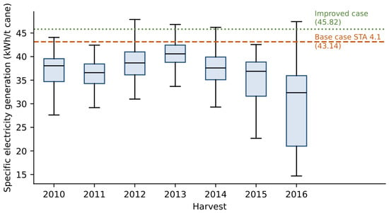
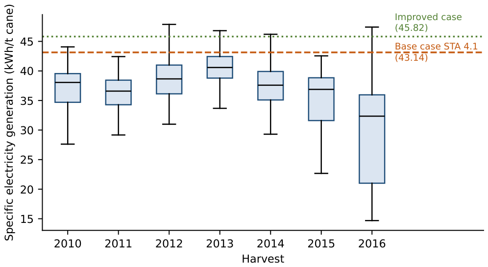
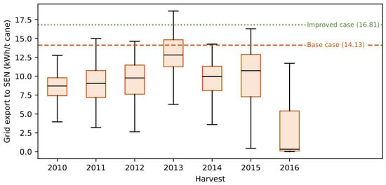
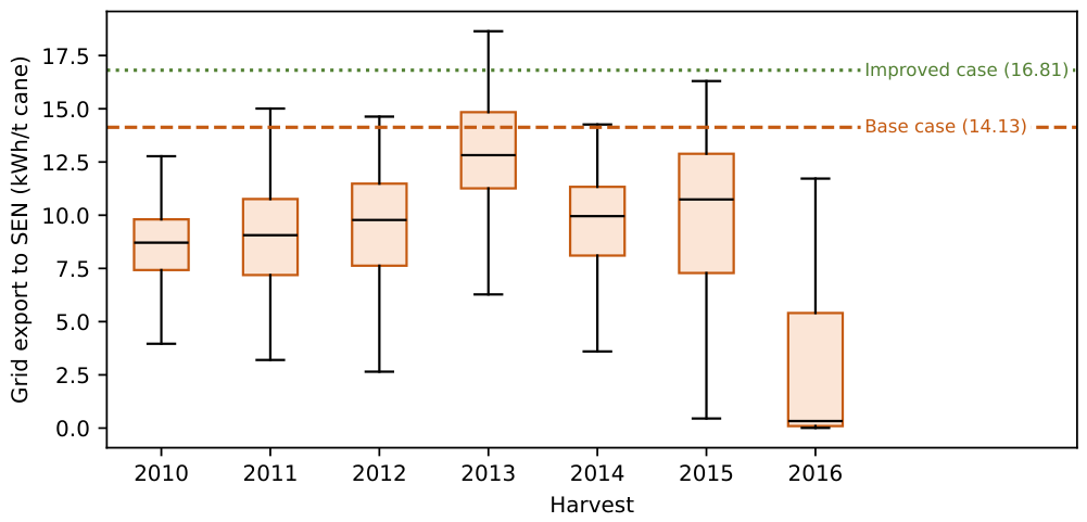
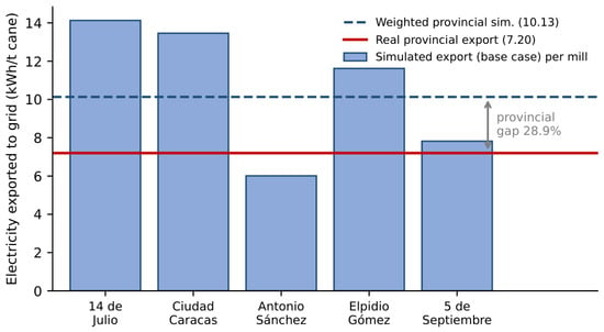
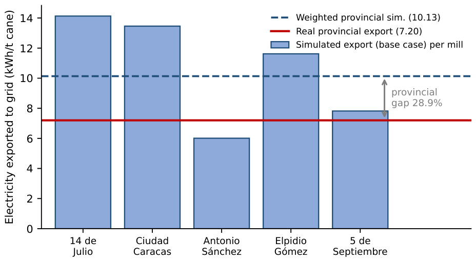
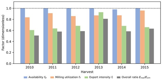
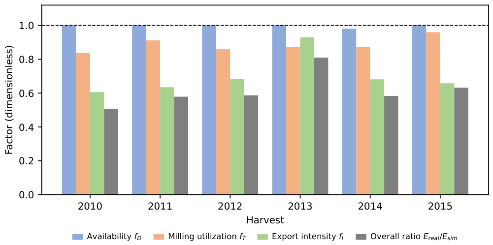
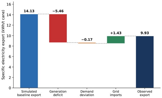
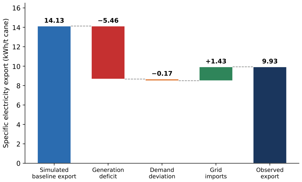
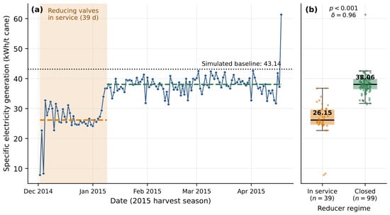
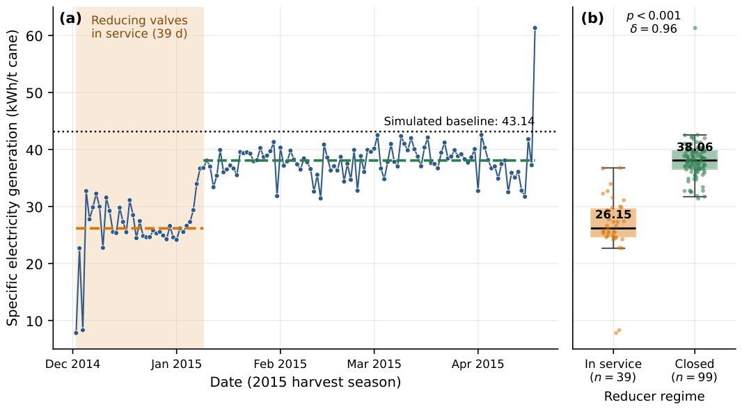
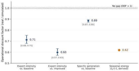
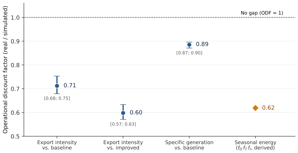

Disclaimer/Publisher’s Note: The statements, opinions and data contained in all publications are solely those of the individual author(s) and contributor(s) and not of MDPI and/or the editor(s). MDPI and/or the editor(s) disclaim responsibility for any injury to people or property resulting from any ideas, methods, instructions or products referred to in the content. |
© 2026 by the authors. Licensee MDPI, Basel, Switzerland. This article is an open access article distributed under the terms and conditions of the Creative Commons Attribution (CC BY) license.