Research on Viscoelastic Nonlinear Energy Sink of Magnetorheological Elastomer for Chatter Suppression in Milling

Abstract

Owing to the low stiffness of thin-walled workpieces, disturbances can readily arise during milling, severely compromising machining accuracy and surface quality. This study proposes a new viscoelastic model of a magnetorheological elastomer (MRE) and analyzes its vibration reduction performance under dynamic cutting forces. First, the governing equations of the system are derived from Newton’s second law, and the amplitude-frequency response curves are obtained using the harmonic balance method. The analytical results are then validated by Runge–Kutta numerical integration, with good agreement between the two approaches. Next, the vibration reduction performance of the MRE-based viscoelastic nonlinear energy sink (MNES) and the effects of its parameters are analyzed. Finally, the nonlinear stiffness coefficient and damping ratio are varied simultaneously at different mass ratios to identify the optimal parameter ranges for the MRE-based viscoelastic nonlinear energy sink of magnetorheological elastomer. The results show that the maximum amplitude of the main system first decreases and then increases as the nonlinear stiffness increases. With appropriate parameter selection, the MRE-based viscoelastic nonlinear energy sink of magnetorheological elastomer provides better vibration reduction performance than the traditional nonlinear energy sink. In addition, as the mass ratio increases, the minimum attainable value of the main-system amplitude initially decreases and then approaches a constant, while the optimal ranges of the nonlinear stiffness coefficient and damping ratio widen slightly. By combining a set of calculated parameters with the differential constitutive equation of the magnetorheological elastomer, the corresponding stress–strain curve is obtained. This provides guidance for the fabrication of magnetorheological elastomers with favorable vibration-damping performance. The stability of milling chatter is also analyzed. The calculated stability lobe diagram and supplementary time-domain verification results show that a milling system with the MNES can effectively suppress chatter and allow a greater depth of cut.

1. Introduction

Chatter is a self-excited vibration influenced by many factors, including the dynamic stiffness of the structure and/or tool, cutting parameters, and workpiece and tool characteristics. It can reduce the dimensional accuracy and surface quality of machined workpieces [1,2,3,4]. This issue is particularly pronounced when machining thin-walled workpieces, for which chatter is a major factor limiting machining efficiency and quality in the production of high-performance components [5,6,7]. Milling chatter is commonly classified as regenerative, mode-coupling, or frictional chatter [8,9]. Among these, regenerative chatter is generally the most prevalent in milling. During multi-tooth interrupted cutting, each tooth removes material from the wavy surface left by the preceding tooth; consequently, the instantaneous chip thickness is governed by both the current vibration and the vibration delayed by one tooth-passing period. This delayed feedback can continuously transfer energy to the structural modes, causing instability when the depth of cut exceeds the stability limit [4,10]. By contrast, mode-coupling chatter originates from asymmetric stiffness or directional coupling in flexible and anisotropic systems, such as long-overhang tools, thin-walled workpieces, and robotic milling systems, and is generally less sensitive to spindle speed [11,12,13,14]. Frictional chatter is primarily associated with flank-face friction, negative damping, and stick-slip effects at low cutting speeds or under conditions involving worn tools or poor lubrication [15,16]. Although these non-regenerative mechanisms may dominate under specific conditions, regenerative chatter remains the most prevalent form of milling chatter, and most stability prediction, monitoring, and suppression strategies have been developed for this mechanism. Therefore, this study focuses on regenerative chatter in milling. Extensive research on milling vibration mechanisms has led to the development of various vibration-suppression methods, which can be broadly classified as passive, active, and semi-active control.

Passive control suppresses vibration by increasing the system’s resistance to vibration through the use of various vibration absorbers [17]. Bolsunovsky et al. [18] designed a tuned mass damper that can be adapted to the frequency response function of a workpiece. Yang et al. [19] considered the effect of material removal during machining and proposed a tuned mass damper for the passive vibration control of thin-walled workpieces. Milling system vibration can also be reduced using specially designed tools and auxiliary support devices. Dong et al. [20] analyzed the stability of a variable-pitch milling cutter and constructed its stability boundary. Experimental results showed that the variable-pitch cutter effectively suppressed milling chatter. Wan et al. [21] proposed a movable auxiliary support structure for low-stiffness thin-walled workpieces to enhance the stiffness and damping of the milling system. Tests conducted with and without the proposed support device verified the feasibility and reliability of the method.

Active suppression methods mainly use sensors to monitor the milling state and piezoelectric or electromagnetic actuators to apply control forces according to prescribed algorithms [22,23]. A novel active control method based on piezoelectric actuators embedded in the tool holder was proposed to suppress milling chatter. During operation, the tool-holder vibration displacement of the tool holder is measured and fed back to a fuzzy controller after the spindle rotation frequency and its harmonic components have been removed. This enables the targeted suppression of the chatter components [24]. Wan et al. [25] proposed an active chatter suppression method based on sliding-mode control and an electromagnetic actuator. The experimental results showed that integrating the electromagnetic actuator improved the stability of the spindle system, demonstrating the robustness and practical applicability of the method.

The complexity, high cost, and high energy consumption of active vibration absorbers limit their practical application [26,27]. Conversely, the fixed parameters of passive vibration absorbers limit their effectiveness under varying operating conditions; in particular, changes in excitation frequency can substantially degrade vibration absorption performance because of detuning. With advances in material development, semi-active vibration suppression methods that combine the advantages of passive and active approaches have emerged. Such methods can improve system stability by adjusting stiffness and damping. Rashid et al. [28] introduced a tuned viscoelastic damper (TVD) for vibration control in milling workpieces. The TVD reduced the vibration acceleration amplitude of the target mode by 20 dB. Oladapo et al. [29] adopted an active-damping approach based on a magnetorheological damper to increase the dynamic structural damping of machine tools without altering the machining operation. Their system combines a vibration absorber with a magnetorheological damper, thereby enlarging the chatter-free region and reducing or potentially eliminating chatter during machining.

A magnetorheological elastomer (MRE) is a composite material characterized by continuously adjustable stiffness and a rapid response [30,31,32,33], making it attractive for semi-active vibration absorbers. MRE-based dynamic vibration absorbers have also received considerable attention owing to their relatively simple structure. Unlike traditional vibration absorbers used solely for passive vibration suppression, the stiffness and damping of an MRE element can be controlled continuously and reversibly by varying the magnetic field’s strength. Therefore, semi-active control can be implemented in response to changes in the vibration load, substantially improving vibration suppression performance. A hybrid MRE vibration absorber can combine nonlinear bandwidth broadening with adaptive frequency-shift characteristics to achieve controllable broadband vibration reduction. Under short-time Fourier transform-based control, such an absorber exhibits lower transmissibility and outperforms a linear vibration absorber [34]. Komatsuzaki et al. [35] proposed an adaptively tunable MRE vibration absorber with self-inductance characteristics. The system uses the self-sensing function of a graphite-based MRE to adjust the natural frequency without external sensors. In precision robotic milling, the low stiffness of industrial robots makes them susceptible to cutting-induced vibration and chatter, which can severely compromise machining quality [14,36,37]. MRE absorbers have therefore been used to attenuate chatter-induced vibration in robotic milling. Experiments under different process parameters and robot configurations have demonstrated their effectiveness and shown significant improvements in workpiece surface quality [38,39,40]. An MRE vibration absorber has also been applied to the milling of thin-walled workpieces to achieve controllable vibration reduction [41].

Various viscoelastic models have been developed to characterize MRE behavior [42,43,44]. However, few studies have incorporated a Kelvin–Voigt element into an MRE viscoelastic model and systematically analyzed the resulting vibration reduction performance. Viscoelastic materials exhibit both viscous and elastic behavior. In addition to their favorable vibration-/noise-reduction and energy-dissipation characteristics, they can be readily fabricated into structures of various sizes and complex shapes. Motivated by these properties, this study investigates an MRE viscoelastic model, derives the system amplitude-frequency response using the harmonic balance method (HBM), and validates the results numerically. Compared with the traditional nonlinear model, the appropriate selection of the MRE viscoelastic parameters can reduce the resonance amplitude and broaden the vibration-reduction frequency band. The effects of these parameters on the main-system response and their optimal ranges for different mass ratios are also investigated. Finally, an availability analysis of the MNES is presented. These findings lay a foundation for the practical use of the MNES in milling chatter suppression.

2. Viscoelastic Nonlinear Energy Sink of Magnetorheological Elastomer

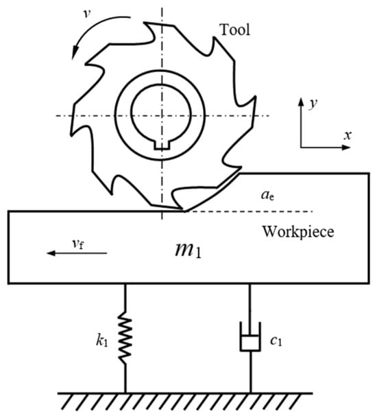
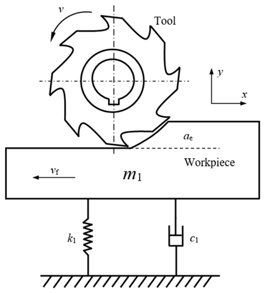
To investigate chatter in a thin-walled workpiece, the milling model shown in Figure 1 is developed. Here, a_p denotes the axial depth of cut. The following assumptions are made to simplify the milling process: (1) the tool is rigid relative to the workpiece; (2) the effect of material removal is neglected; and (3) the workpiece vibrates only in the y direction.

Figure 1. Milling chatter model for a thin-walled workpiece.

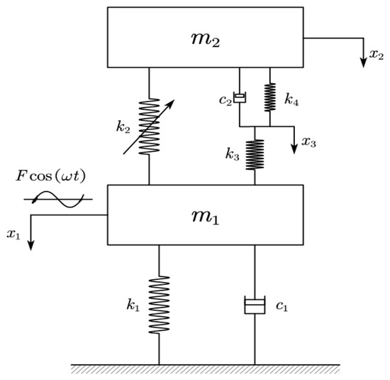
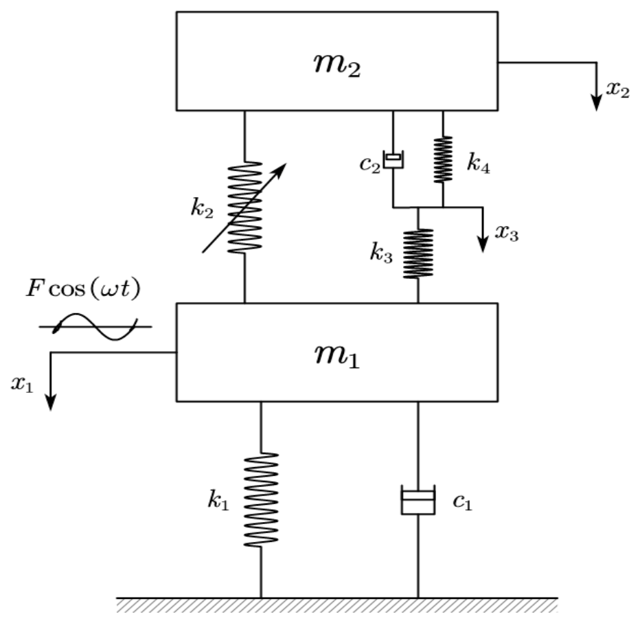
To suppress chatter in the thin-walled workpiece, the MRE viscoelastic model developed in this study is configured as shown in Figure 2 and is hereafter referred to as the viscoelastic nonlinear energy sink of magnetorheological elastomer (MNES). Here, m₁ represents the mass of the main-system oscillator; k₁ and c₁ are the linear stiffness and damping coefficients of the main-system oscillator, respectively; k₂ is the cubic stiffness coefficient of the MNES; c₂ is the linear damping coefficient of the MNES; and k₃ and k₄ are the linear stiffness coefficients of the MNES.

Figure 2. Mechanical model of the viscoelastic nonlinear energy sink.

In the parametric modeling of MREs, the cubic stiffness term is introduced to characterize nonlinear mechanical behavior under large deformations or displacements. It is typically formulated by adding a term proportional to the cube of the displacement cubed to the restoring-force expression. The cubic stiffness coefficient is central to the parametric modeling of MREs, and its magnitude is governed by the magnetic-field strength. In this study, k₂ is parameterized, whereas magnetic field control is not modeled quantitatively.

This study adopts linear regenerative chatter theory. Near the stability boundary, the vibration amplitude remains small and contact between the cutting teeth and the workpiece is maintained, indicating weakly nonlinear system behavior. In the regenerative chatter model, the instantaneous variation in uncut chip thickness is governed by the difference between the current and delayed relative vibrations of the tool and the workpiece. Let y(t) denote the relative vibration in the chip-thickness direction and T the regeneration delay, i.e., the tooth-passing period or spindle revolution period. The dynamic variation in chip thickness is then expressed as [45]

$$\Delta h(t)=y(t)-y(t-T)$$

(1)

The dynamic cutting force is assumed to be proportional to the dynamic uncut chip thickness:

$$\Delta F(t)=K_{\mathrm{c}}{a}_{\mathrm{p}}{B}_0\Delta h(t)$$

(2)

where K_c is the cutting force coefficient, a_p is the axial depth of cut, and B₀ is the average directional factor, which is treated here as a scalar constant. Substituting Equation (1) into Equation (2) yields

$$\Delta F(t)=K_{\mathrm{c}}{a}_{\mathrm{p}}{B}_0\left[y(t)-y(t-T)\right]$$

(3)

For a harmonic relative vibration x(t) = A₀cos(ωt), the delayed term is x(t − T) = A₀cos(ωt − ωT). Substituting these expressions into the dynamic cutting force equation and applying a trigonometric identity yields

$$\Delta F(t)=2K_{\mathrm{c}}{a}_{\mathrm{p}}{B}_0{A}_{0}sin({\displaystyle \frac{\omega T}{2}})cos\left(\omega t-{\displaystyle \frac{\omega T}{2}}+{\displaystyle \frac{\pi }{2}}\right)$$

(4)

Under the cutting force sign convention adopted in Equation (3), the cycle-averaged mechanical power associated with the regenerative force is

$$\overline{P}={\displaystyle \frac{1}{2}}{K}_{\mathrm{c}}{a}_{\mathrm{p}}{B}_0{A}_0^2\omega sin(\omega T)$$

(5)

This dynamic force can supply energy to the vibration system and thereby promote regenerative chatter when the phase relationship is favorable. In particular, the average power reaches its maximum positive value when sin(ωT) = 1, i.e., ωT = π/2 + 2jπ with j = 0, 1, 2,…, so the regenerative force amplitude is |△F(t)|_max = $\sqrt{2}$K_ca_pB₀A₀. At this condition, the average power reaches its maximum, the negative damping effect is strongest, and chatter is most likely to occur. Since the initial phase only shifts the time origin and does not affect the amplitude, frequency, or relative phase in the regenerative chip-thickness variation, it can be set to zero without loss of generality. Accordingly, setting F =$\sqrt{2}$K_ca_pB₀A₀ allows Equation (4) to be written as

$$\Delta F(t)=Fcos(\omega t)$$

(6)

where F and ω denote the amplitude and frequency of the dynamic cutting force, respectively. The variables x₁ and x₂ denote the displacements of the two masses, while x₃ denotes the displacement at the junction of the two linear springs in the MNES. The governing equations of the system are

$$\left\{\begin{array}{l}{m}_1{\ddot{x}}_1+c_1{\dot{x}}_1+k_1{x}_1+k_2{(x_1-x_2)}^3+k_3(x_1-x_3)=Fcos(\omega t)\\ m_2{\ddot{x}}_2+c_2({\dot{x}}_2-{\dot{x}}_3)+k_4(x_2-x_3)+k_2{(x_2-x_1)}^3=0\\ k_3(x_3-x_1)+c_2({\dot{x}}_3-{\dot{x}}_2)+k_4(x_3-x_2)=0\end{array}\right.$$

(7)

For the prescribed-force frequency-response analysis in Section 3, Section 4 and Section 5, the cutting action is represented by an independent harmonic excitation Fcos(ωt), where F is a specified amplitude. This idealization is used to evaluate forced-vibration attenuation and is not equivalent to retaining the displacement-dependent regenerative feedback. The full delayed-force model is introduced separately in Section 6.2 for chatter stability analysis.

The following transformation is introduced:

$$\begin{array}{l}{\omega }_1^2={\displaystyle \frac{k_1}{m_1}},{\lambda }_1={\displaystyle \frac{c_1}{2m_1{\omega }_1}},{\lambda }_2={\displaystyle \frac{c_2}{2m_1{\omega }_1}},\mu ={\displaystyle \frac{m_2}{m_1}},\gamma ={\displaystyle \frac{\omega }{{\omega }_1}},\\ {\alpha }_1={\displaystyle \frac{k_2}{k_1}},{\alpha }_2={\displaystyle \frac{k_3}{k_1}},{\alpha }_3={\displaystyle \frac{k_4}{k_1}},f={\displaystyle \frac{F}{k_1}},\tau ={\omega }_{1}t\end{array}$$

Here, α₁ denotes the normalized nonlinear stiffness coefficient and has units of m⁻², whereas α₂ and α₃ denote dimensionless linear stiffness ratios. Equation (7) can then be rewritten as

$$\left\{\begin{array}{l}{\ddot{x}}_1+2{\lambda }_1{\dot{x}}_1+x_1+{\alpha }_1{(x_1-x_2)}^3+{\alpha }_2(x_1-x_3)=fcos(\gamma \tau )\\ \mu {\ddot{x}}_2+2{\lambda }_2({\dot{x}}_2-{\dot{x}}_3)+{\alpha }_1{(x_2-x_1)}^3+{\alpha }_3(x_2-x_3)=0\\ {\alpha }_2(x_3-x_1)+{\alpha }_3(x_3-x_2)+2{\lambda }_2({\dot{x}}_3-{\dot{x}}_2)=0\end{array}\right.$$

(8)

3. Harmonic Balance Method Solution and Numerical Verification

To further investigate the effects of the system parameters and the vibration reduction performance of the MNES, the HBM is used to determine the system’s amplitude-frequency response. Accordingly, the vibration response of Equation (8) is approximated by a finite harmonic expansion

$$\begin{array}{l}{x}_1=a_{11}cos(\gamma \tau )+b_{11}sin(\gamma \tau )\\ x_2=a_{12}cos(\gamma \tau )+b_{12}sin(\gamma \tau )\\ x_3=a_{13}cos(\gamma \tau )+b_{13}sin(\gamma \tau )\end{array}$$

(9)

where a_1j and b_1j (j = 1, 2, 3) are the harmonic coefficients to be determined.

Substituting Equation (9) into Equation (8), neglecting high-order terms, and equating the coefficients of cos(γτ) and sin(γτ) gives the following set of nonlinear algebraic equations:

$$\begin{array}{l}-4f+3{\alpha }_1{a}_{11}^3-9{\alpha }_1{a}_{12}{a}_{11}^2-3{\alpha }_1{a}_{12}\left[a_{12}^2+{(b_{11}-b_{12})}^2\right]-4{\alpha }_2{a}_{13}\\ +8\gamma {\lambda }_1{b}_{11}+a_{11}\left[9{\alpha }_1{a}_{12}^2+3{\alpha }_1{(b_{11}-b_{12})}^2+4(1+{\alpha }_2-{\gamma }^2)\right]=0\\ 3{\alpha }_1{b}_{11}^3-9{\alpha }_1{b}_{12}{b}_{11}^2-3{\alpha }_1{b}_{12}\left[b_{12}^2+{(a_{11}-a_{12})}^2\right]-4{\alpha }_2{b}_{13}\\ -8\gamma {\lambda }_1{a}_{11}+b_{11}\left[9{\alpha }_1{b}_{12}^2+3{\alpha }_1{(a_{11}-a_{12})}^2+4(1+{\alpha }_2-{\gamma }^2)\right]=0\\ -{\displaystyle \frac{3}{4}}{\alpha }_1(a_{11}-a_{12})\left[{(a_{11}-a_{12})}^2+{(b_{11}-b_{12})}^2\right]\\ +2\gamma {\lambda }_2(b_{12}-b_{13})+{\alpha }_3(a_{12}-a_{13})-a_{12}{\gamma }^2\mu =0\\ -{\displaystyle \frac{3}{4}}{\alpha }_1(b_{11}-b_{12})\left[{(a_{11}-a_{12})}^2+{(b_{11}-b_{12})}^2\right]\\ +2\gamma {\lambda }_2(-a_{12}+a_{13})+{\alpha }_3(b_{12}-b_{13})-b_{12}{\gamma }^2\mu =0\\ -{\alpha }_2{a}_{11}+{\alpha }_2{a}_{13}+{\alpha }_3(-a_{12}+a_{13})+2\gamma {\lambda }_2(-b_{12}+b_{13})=0\\ -{\alpha }_2{b}_{11}+{\alpha }_2{b}_{13}+{\alpha }_3(-b_{12}+b_{13})+2\gamma {\lambda }_2(a_{12}-a_{13})=0\end{array}$$

(10)

The resulting main-system amplitude-frequency response is

$$\begin{array}{l}{x}_{1\mathrm{w}}=\sqrt{a_{11}^2+b_{11}^2}\\ x_{2\mathrm{w}}=\sqrt{a_{12}^2+b_{12}^2}\\ x_{3\mathrm{w}}=\sqrt{a_{13}^2+b_{13}^2}\end{array}$$

(11)

Equation (10) contains nonlinear coupling among the amplitudes, making a closed-form analytical solution difficult to obtain. Therefore, the MATLAB (ver. R2025b) fsolve function is used to solve the nonlinear algebraic system in Equation (10) numerically. When solving Equation (10) with fsolve, the current solution serves as the initial guess for the next iteration, the frequency increment is 0.05 rad/s, and a forward frequency sweep is adopted. The residual norm, condition number of the Jacobian, determinant of the Jacobian, and eigenvalues of the Jacobian are examined to identify possible multiple roots.

The five-dimensional state formulation follows from eliminating the velocity of the massless intermediate junction. The third equation of Equation (7) gives

$${\dot{x}}_3={\dot{x}}_2-{\displaystyle \frac{1}{c_2}}\left[k_3(x_3-x_1)+k_4(x_3-x_2)\right]$$

(12)

Substituting this expression into the second-mass equation yields

$${\ddot{x}}_2={\displaystyle \frac{1}{m_2}}\left[k_3(x_1-x_3)-k_2{(x_2-x_1)}^3\right]$$

(13)

Define the state vector as

$$\mathit{z}=\left[\begin{array}{l}{z}_1\hfill \\ z_2\hfill \\ z_3\hfill \\ z_4\hfill \\ z_5\hfill \end{array}\right]=\left[\begin{array}{l}{x}_1\hfill \\ {\dot{x}}_1\hfill \\ x_2\hfill \\ {\dot{x}}_2\hfill \\ x_3\hfill \end{array}\right]$$

(14)

Then, Equation (7) can then be written as the following first-order system:

$$\left\{\begin{array}{l}{\dot{z}}_1=z_2\hfill \\ {\dot{z}}_2={\displaystyle \frac{1}{m_1}}\left[Fcos(\omega t)-c_1{z}_2-k_1{z}_1-k_3(z_1-z_5)-k_2{(z_1-z_3)}^3\right]\hfill \\ {\dot{z}}_3=z_4\hfill \\ {\dot{z}}_4={\displaystyle \frac{1}{m_2}}\left[k_3(z_1-z_5)-k_2{(z_3-z_1)}^3\right]\hfill \\ {\dot{z}}_5=z_4-{\displaystyle \frac{1}{c_2}}\left[k_3(z_5-z_1)+k_4(z_5-z_3)\right]\hfill \end{array}\right.$$

(15)

Numerical integration is performed using the MATLAB ode45 solver. The relative and absolute tolerances are set to 1 × 10⁻⁶ and 1 × 10⁻⁸, respectively. To remove transient effects, the first 70% of each time series is discarded. Then, the amplitude is calculated by dividing the peak-to-peak value of the last 30% of the sampling points by 2. The initial conditions are specified as [0, 0, 0, 0, 0]. Because ode45 uses a variable-step solver, the prescribed tolerances automatically control the step size.

With Equation (14), this is precisely the fourth first-order equation in Equation (15). The remaining state equations follow directly from the primary-mass equation and the junction relation. Thus, Equation (15) is algebraically equivalent to Equation (7) for the stated network, provided that c2 > 0.

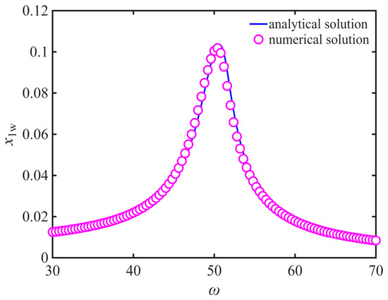
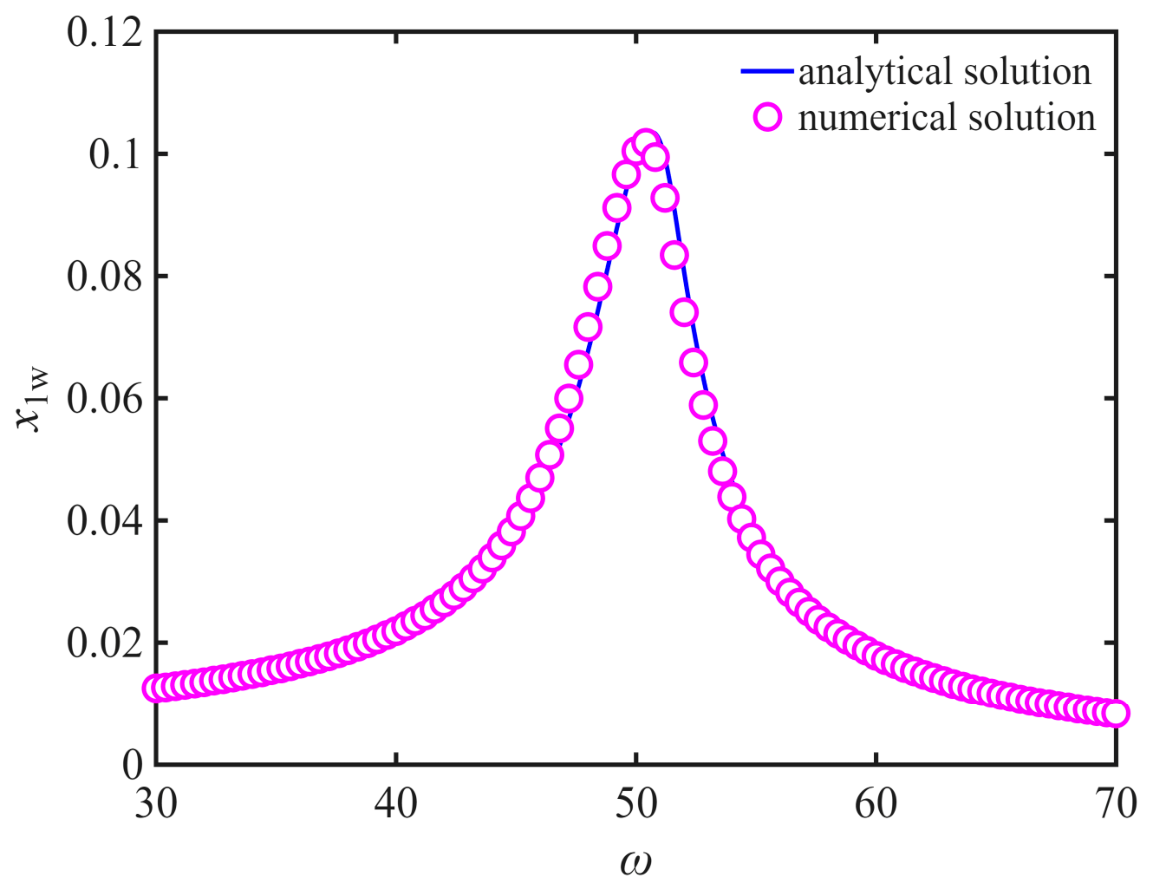
A Runge–Kutta time-integration scheme implemented in MATLAB is used to validate the harmonic-balance results. The selected parameters are m₁ = 4 kg, m₂ = 0.4 kg, c₁ = 12 N⋅s/m, c₂ = 12 N⋅s/m, k₁ = 1 × 10⁴ N/m, k₂ = 1 × 10⁴ N/m³, k₃ = 1 × 10³ N/m, k₄= 1 × 10² N/m, and F = 80 N. The main-system amplitude-frequency response curves obtained from Equation (15) using these parameters are shown in Figure 3. The numerical response shows good agreement with the HBM results, thereby validating the harmonic-balance solution. Accordingly, the HBM is used for subsequent parametric analyses.

Figure 3. Comparison of the main-system amplitude-frequency response curves obtained by using the HBM and numerical integration.

A multi-start search strategy was used to identify multiple solution branches. At each value of ω, multiple initial guesses were used, with the solution from the preceding ω retained as a warm start, and fsolve was used to obtain all converged and mutually distinct solutions. The computations were performed at F = 80 N. The results indicate that no multiple solution branches, turning points, or hysteresis phenomena were observed.

The parameters adopted in the forced-response calculations are intended for the theoretical comparison of vibration-attenuation trends rather than for a calibrated prediction of the displacement of a particular milled thin-walled workpiece. For the MNES with m₁ = 4 kg, k₁ =1 × 10⁴ N/m, and c₁ = 12 N s/m, the undamped natural frequency is ω_n = 50 rad/s. Under the prescribed force amplitude F = 80 N, the single-degree-of-freedom resonant-amplitude estimate without NES is F/(c₁ω_n) ≈ 0.133 m. This large dimensional reference response reflects the chosen force and structural compliance and should not be treated as a measured or representative displacement during practical milling. Accordingly, the present frequency-response results primarily support comparative conclusions under matched model assumptions.

4. Vibration Reduction Performance Analysis of the Viscoelastic Nonlinear Energy Sink

The MNES replaces the damping element of the traditional nonlinear energy sink (TNES) with a viscoelastic Kelvin–Voigt element connected in series with a linear spring. This section assesses the vibration reduction performance of the MNES and examines the effects of its parameters on the main-system response.

This section examines the reduction of the primary-system response under a prescribed harmonic input Fcos(ωt) and compares the viscoelastic MNES with the traditional NES under identical excitation conditions. The resulting resonance amplitudes and frequency-response bandwidths characterize forced-vibration attenuation. They should not be interpreted as direct proof of regenerative chatter suppression because the imposed harmonic load does not retain the delayed displacement feedback of the milling process. Chatter stability is evaluated separately in Section 6.2 using the regenerative-delay equation.

4.1. Effect of Nonlinear Stiffness k₂

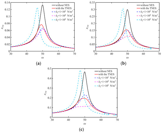
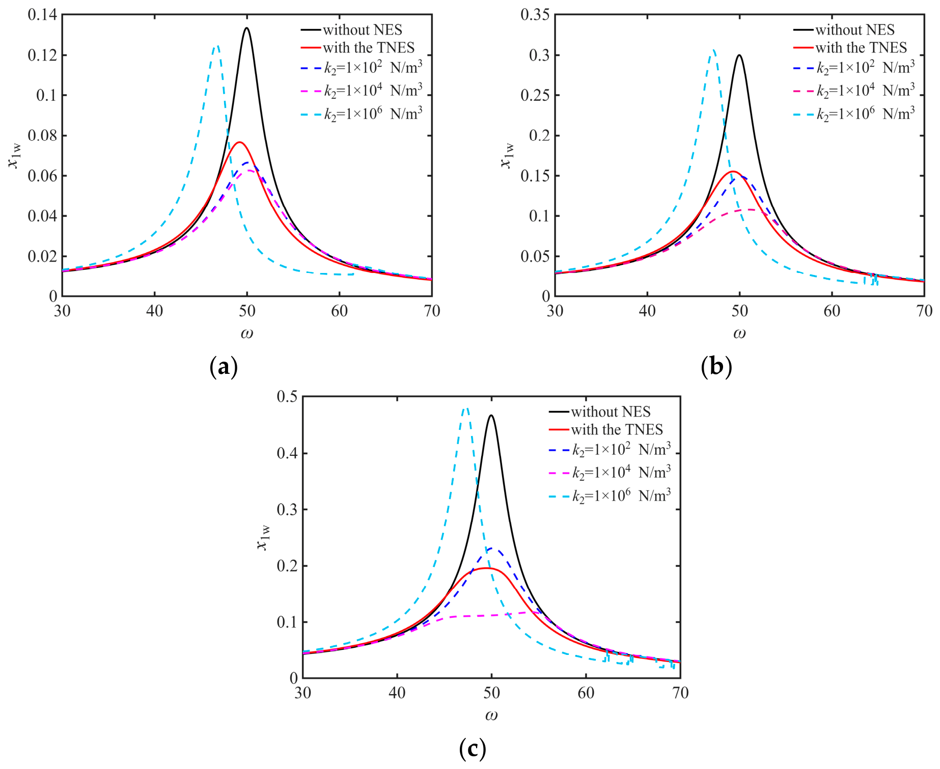
According to Ref. [46], for a linear oscillator with mass m₁ = 4 kg, linear stiffness k₁ = 1 × 10⁴ N/m, and damping c₁ = 5 N⋅s/m, a traditional NES with m₂ = 0.4 kg, cubic nonlinear stiffness k₂ = 1 × 10⁵ N/m³, and damping c₂ = 5 N⋅s/m provides enhanced damping and good system robustness. For the model in Figure 2, the selected primary-oscillator parameters are m₁ = 4 kg, k₁ =1 × 10⁴ N/m, and c₁ = 12 N·s/m, while the selected MNES parameters are m₂ = 0.4 kg, k₃ = 1 × 10³ N/m, k₄ = 1 × 10² N/m, and c₂ = 12 N·s/m. The corresponding dimensionless parameters are μ = 0.1, α₂ = 0.1, α₃ = 0.01, and λ₂ = 0.03. For these conditions, Figure 4 shows the main-system amplitude-frequency response curves for k₂ values of 1 × 10² N/m³, 1 × 10⁴ N/m³ and 1 × 10⁶ N/m³ under different excitation amplitudes, together with the TNES response for k₂ = 1 × 10⁴ N/m³. Here, NES denotes nonlinear energy sink. As shown in Figure 4, when the nonlinear stiffness of the MNES is k₂ = 1 × 10⁴ N/m³, corresponding to α₁ = 1 m⁻², the main system exhibits good robustness. Moreover, the resonance amplitude first decreases and then increases as the nonlinear stiffness increases. When k₂ = 1 × 10⁴ N/m³ and the damping ratio λ₂ is small, the MNES provides slightly better vibration reduction performance than the TNES under the different excitation amplitudes considered.

Figure 4. Main-system amplitude-frequency response curves for different values of F and k₂: (a) F = 80 N. (b) F = 180 N. (c) F = 280 N.

Therefore, the nonlinear stiffness coefficient α₁ of the MNES is set to 1 m⁻² in the subsequent analysis.

4.2. Analysis of Linear Stiffness Ratio

4.2.1. Effect of the Linear Stiffness Ratio α₂

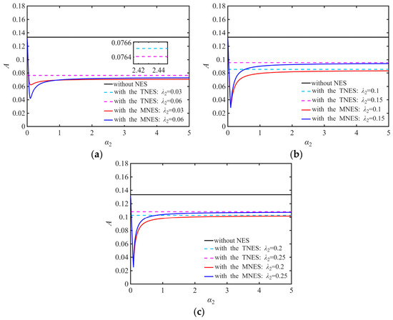
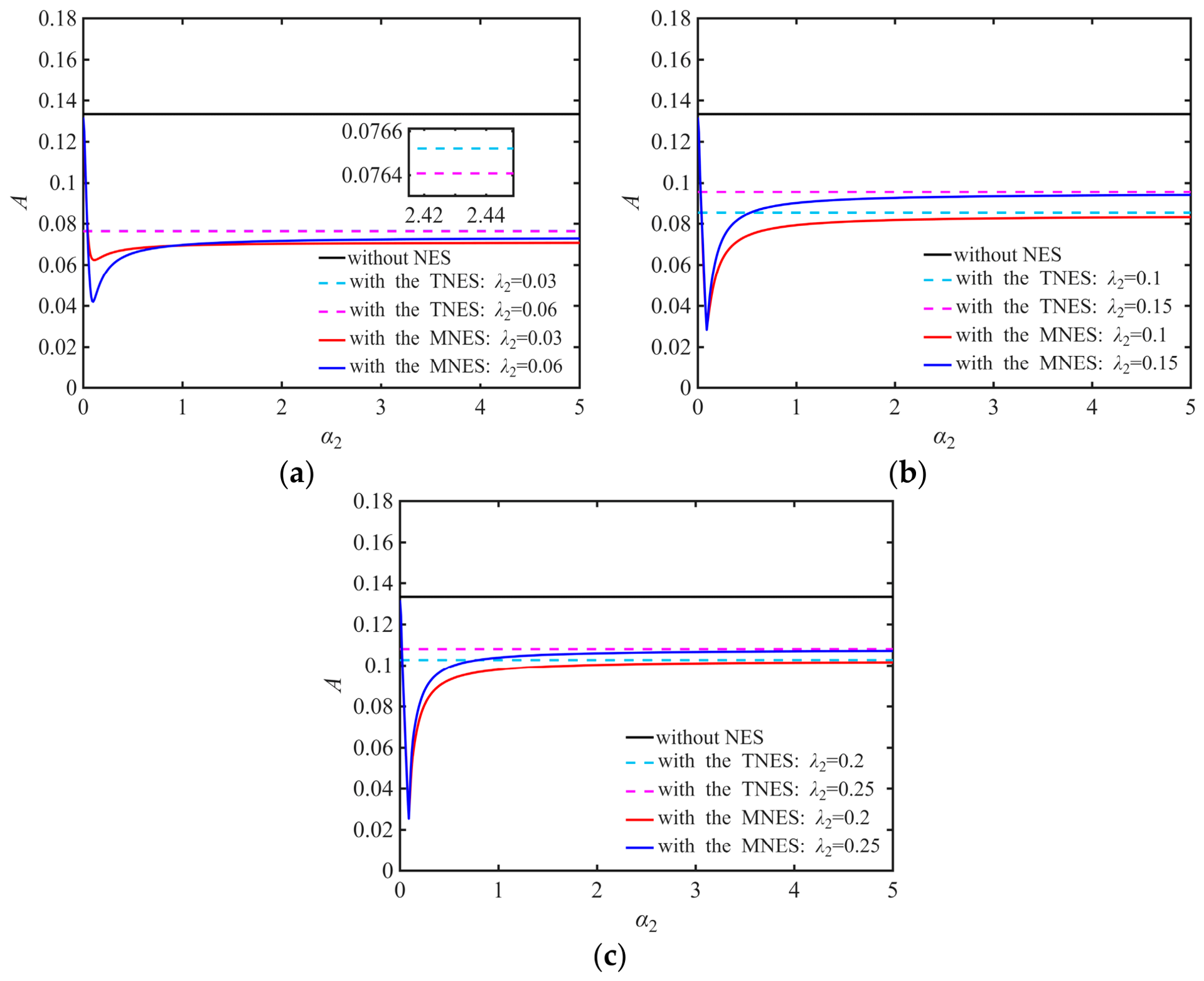
Based on Section 4.1, the selected dimensionless parameters of the MRE system are μ = 0.1, α₁ = 1 m⁻², λ₁ = 0.03, α₃ = 0.01, and f = 0.008. A series of main-system amplitude-frequency response curves is obtained for different values of α₂ and λ₂. Figure 5 shows the maximum response amplitude as a function of the linear stiffness ratio for different damping ratios, where A denotes the maximum amplitude of the calculated main-system frequency response. The results indicate that the MNES outperformed the TNES for most of the parameter combinations considered.

Figure 5. Variation in the maximum amplitude with stiffness ratio α₂: (a) λ₂ = 0.03 and 0.06. (b) λ₂ = 0.1 and 0.15. (c) λ₂ = 0.2 and 0.25.

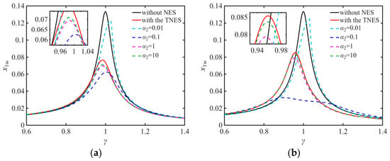
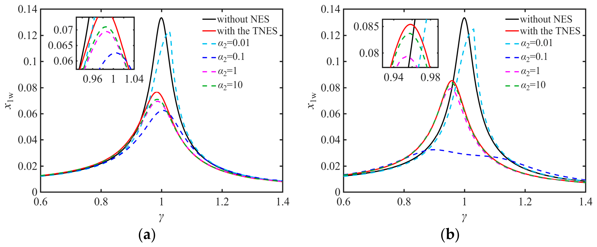
To further examine the main-system response, Figure 6 presents the amplitude-frequency response curves for different stiffness ratios α₂ with λ₂ set to 0.03 and 0.1. When α₂ = 0.1, the main-system exhibits the smallest vibration amplitude and the widest vibration-reduction frequency band. Figure 5 and Figure 6 show that, as α₂ increases, the peak response initially decreases, then increases, and finally approaches a nearly constant value. When λ₂ < 0.2, an excessively small α₂ results in poorer vibration reduction performance for the MNES than for the TNES. Regardless of λ₂, when α₂ becomes sufficiently large, the vibration reduction performance of the MNES approaches that of the TNES. Overall, for the damping ratios considered, the main-system vibration amplitude is minimized near α₂ = 0.1; therefore, α₂ = 0.1 is adopted in the following analysis.

Figure 6. Main-system amplitude-frequency response curves for different α₂ and λ₂: (a) λ₂ = 0.03. (b) λ₂ = 0.1.

4.2.2. Effect of the Linear Stiffness Ratio α₃

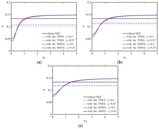
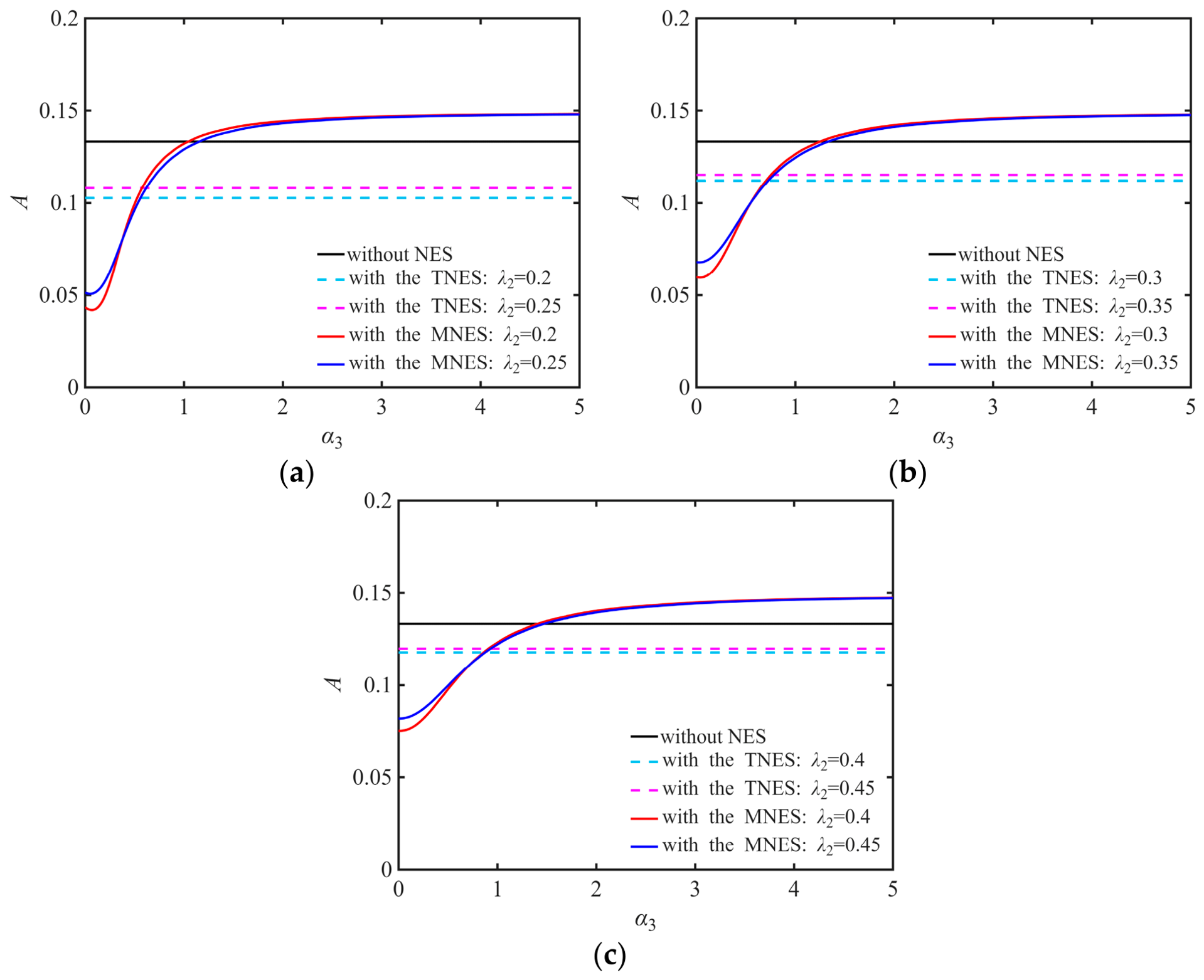
Based on Section 4.1, the selected dimensionless parameters of the MRE system are μ= 0.1, α₁ = 1 m⁻², α₂ = 0.1, λ₁ = 0.03, and f = 0.008. A series of main-system amplitude-frequency response curves is obtained for different values of α₃ and λ₂. Figure 7 shows the maximum response amplitude as a function of the linear stiffness ratio for different damping ratios, where A denotes the maximum amplitude of the calculated main-system frequency response. The results indicate that the MNES outperforms the TNES for most of the parameter combinations considered.

Figure 7. Variation in the maximum amplitude with stiffness ratio α₃: (a) λ₂ = 0.2 and 0.25. (b) λ₂ = 0.3 and 0.35. (c) λ₂ = 0.4 and 0.45.

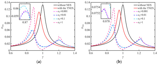
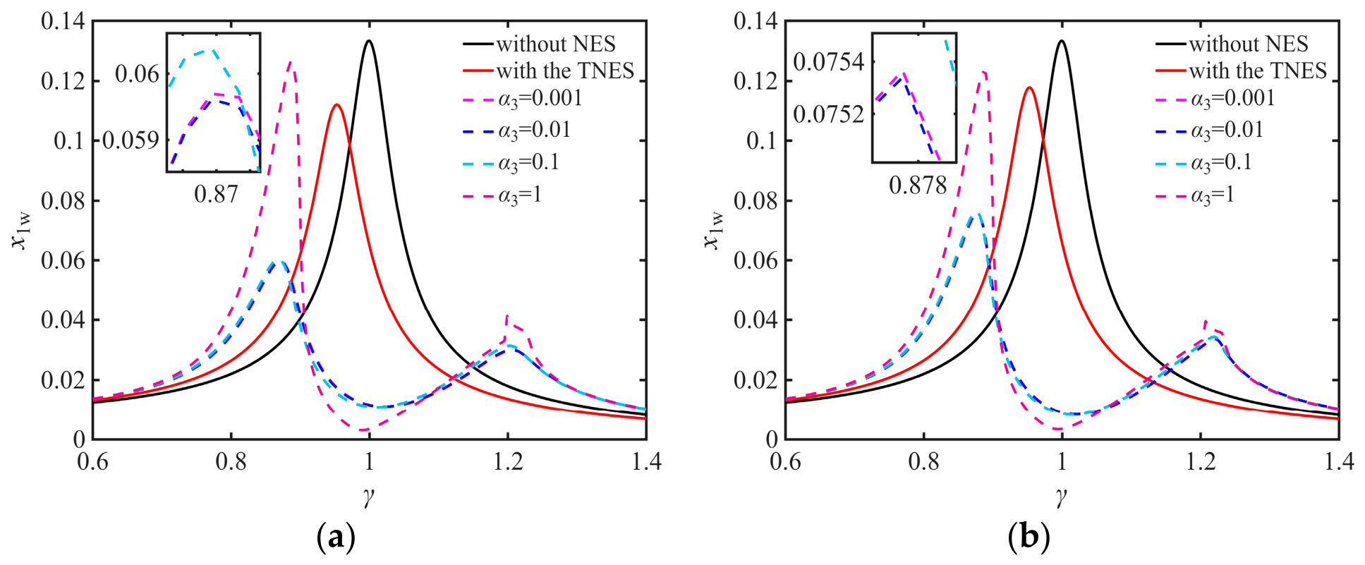
To further examine the main-system response, Figure 8 presents the amplitude-frequency response curves for different stiffness ratios α₃ for λ₂ values of 0.3 and 0.4. When α₃ = 0.01, the main system exhibits the smallest vibration amplitude and the widest vibration-reduction frequency band. Figure 7 and Figure 8 show that, as α₃ increases, the peak response initially decreases, then increases, and finally remains nearly constant. When λ₂ < 0.4, an excessively small α₃ results in poorer vibration reduction performance for the MNES than for the TNES. Regardless of λ₂, when α₃ becomes sufficiently large, the vibration reduction performance of the MNES approaches that of the TNES. Overall, for the damping ratios considered, the main-system vibration amplitude is minimized near α₃ = 0.01; therefore, α₃ = 0.01 is adopted in the following analysis.

Figure 8. Main-system amplitude-frequency response curves for different α₃ and λ₂: (a) λ₂ = 0.3. (b) λ₂ = 0.4.

4.3. Effect of the Damping Ratio

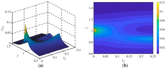
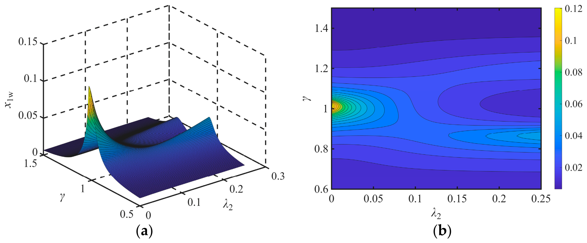
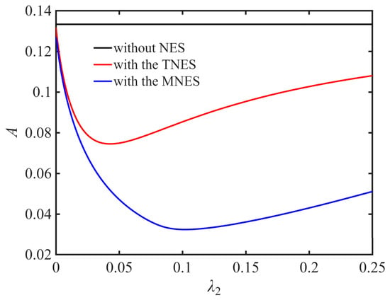
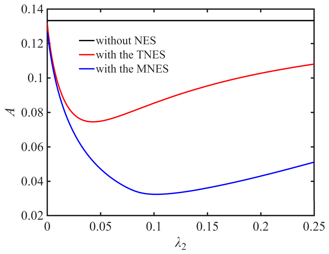
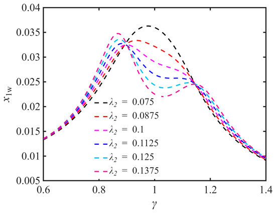
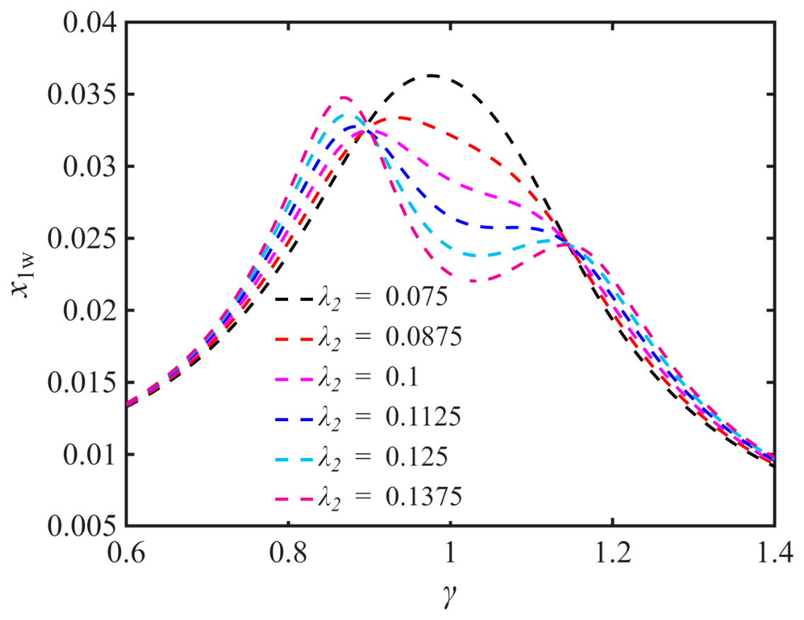
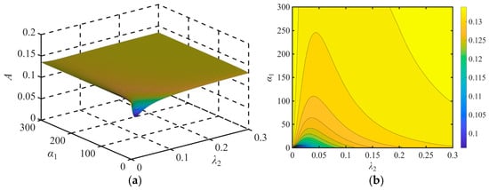
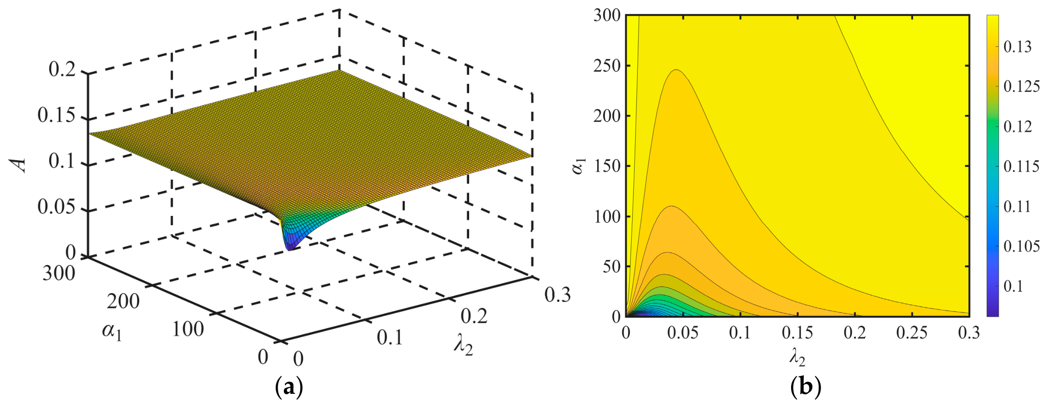
The selected dimensionless parameters of the MRE system are μ = 0.1, α₁ = 1 m⁻², α₂ = 0.1, α₃ = 0.01, λ₁ = 0.03, and f = 0.008. Figure 9 presents a three-dimensional surface plot and a two-dimensional contour plot of the main-system amplitude-frequency response as λ₂ varies. As λ₂ increases, the main-system response changes from a single-peaked to a double-peaked response, while the resonance region amplitude first decreases and then increases. Therefore, an optimal damping ratio λ₂ exists that minimizes the resonance amplitude of the main system. Figure 10 shows the calculated maximum amplitude A of the TNES and MNES as functions of λ₂. Both types of NES reduce the resonance peak of the main system, but the MNES achieves greater vibration reduction than the TNES. Within a certain range of damping ratios, the performance difference between the TNES and MNES increases with λ₂. Figure 11 shows the amplitude-frequency response curves of the MNES for different values of λ₂. Figure 10 and Figure 11 show that the MNES resonance amplitude first decreases and then increases as the damping ratio increases, reaching a minimum at λ₂ = 0.1.

Figure 9. Main-system amplitude-frequency response for varying λ₂: (a) three-dimensional surface plot; (b) a two-dimensional contour plot.

Figure 10. Variation in the maximum amplitude with λ₂.

Figure 11. MNES amplitude-frequency response curves for different values of λ₂.

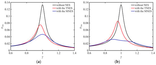
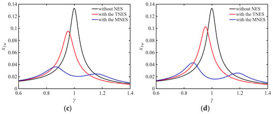
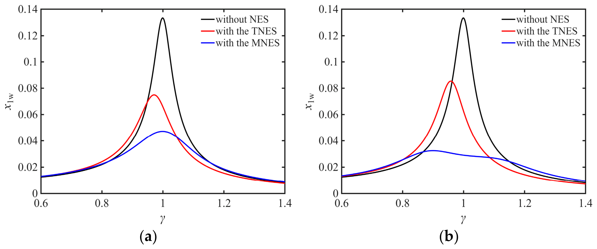
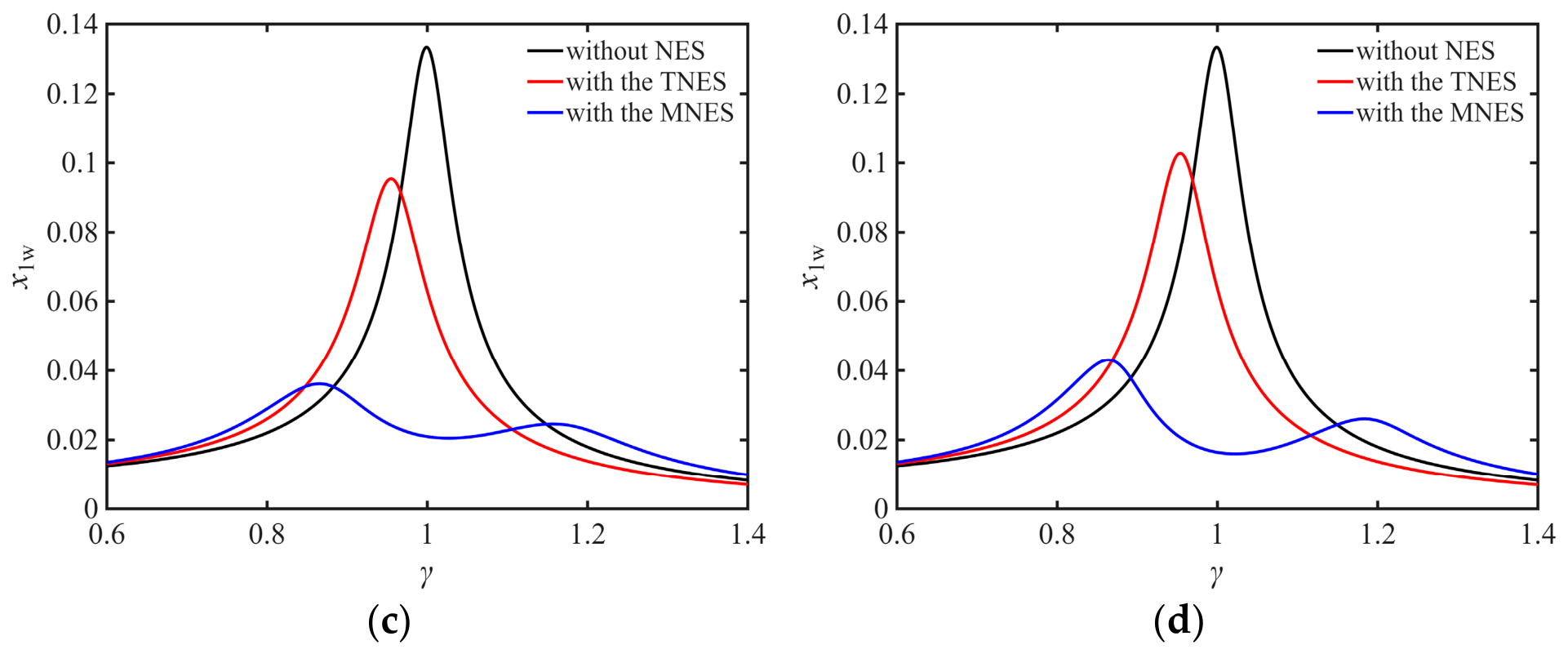
To compare the vibration reduction performance of the two NES configurations, Figure 12 presents their amplitude-frequency response curves at different damping ratios. At the same damping ratio, the MNES achieves a greater reduction in the main-system resonance amplitude than the TNES and provides a wider vibration-reduction frequency band. Therefore, selecting an appropriate damping ratio is important for improving vibration reduction performance.

Figure 12. Comparison of the vibration reduction performance of the two nonlinear energy sinks at different λ₂: (a) λ₂ = 0.05. (b) λ₂ = 0.10. (c) λ₂ = 0.15. (d) λ₂ = 0.20.

5. Optimal Parameter Range of the Viscoelastic Nonlinear Energy Sink

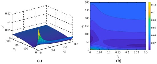
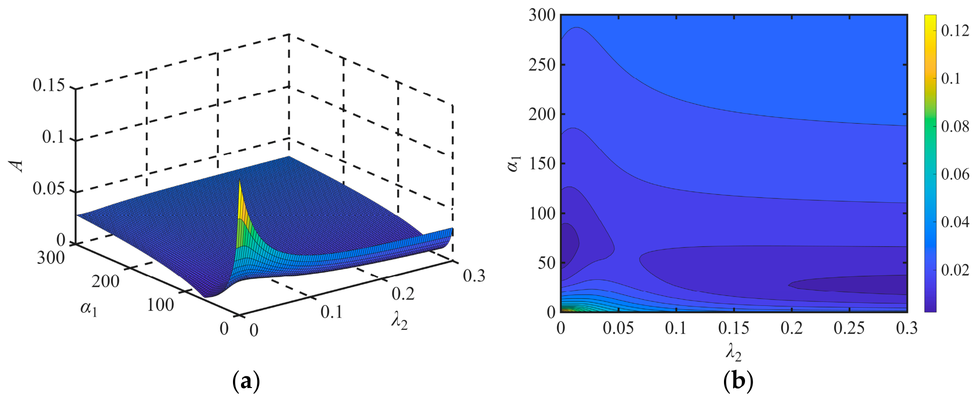
Section 4 examined the effects of the MNES parameters on the system amplitude-frequency response. For each selected mass ratio, the linear stiffness ratio α₂ is fixed, while the nonlinear stiffness coefficient α₁ and damping ratio λ₂ are varied simultaneously to obtain a set of amplitude-frequency response curves. The maximum amplitude A is then determined to evaluate vibration reduction performance and identify the optimal parameter ranges.

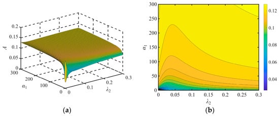
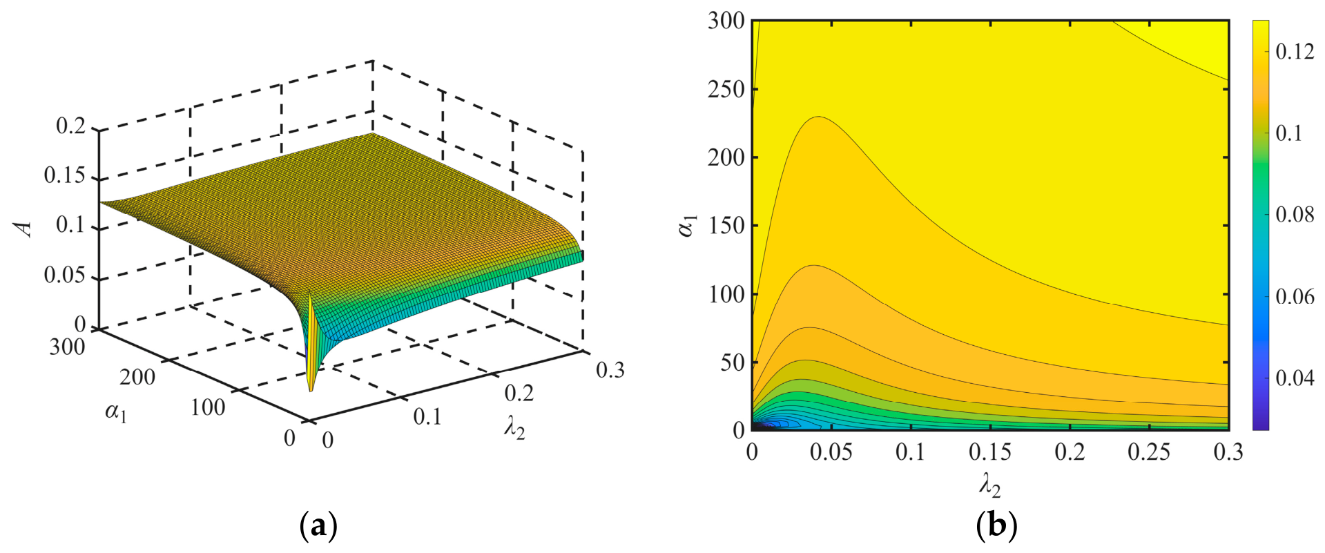
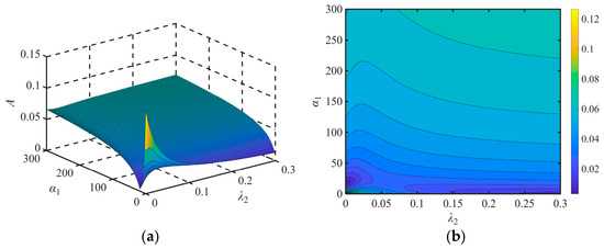
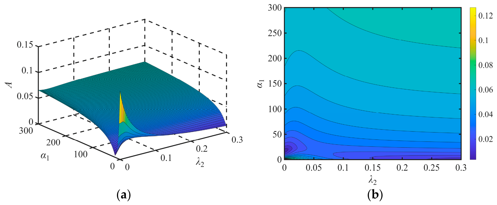
For mass ratios μ = 0.025, 0.05, 0.1, and 0.15, α₁ and λ₂ are varied simultaneously, and the resulting maximum main-system response amplitudes are shown in Figure 13, Figure 14, Figure 15 and Figure 16. The optimal parameter range and the achievable vibration reduction both depend on the mass ratio. For μ = 0.025 (Figure 13), the maximum main-system amplitude within the optimal MNES parameter range is approximately 0.1. At μ = 0.05, this value decreases to approximately 0.04 (Figure 14). For μ = 0.1 and 0.15 (Figure 15 and Figure 16, respectively), the maximum main-system amplitude is approximately 0.02. Vibration reduction performance deteriorates when either parameter is excessively small or excessively large.

Figure 13. Maximum main-system amplitude as a function of α₁ and λ₂ (μ = 0.025): (a) three-dimensional surface plot; (b) two-dimensional contour plot.

Figure 14. Maximum main-system amplitude as a function of α₁ and λ₂ (μ = 0.05): (a) three-dimensional surface plot; (b) two-dimensional contour plot.

Figure 15. Maximum main-system amplitude as a function of α₁ and λ₂ (μ = 0.1): (a) three-dimensional surface plot; (b) two-dimensional contour plot.

Figure 16. Maximum main-system amplitude as a function of α₁ and λ₂ (μ = 0.15): (a) three-dimensional surface plot; (b) two-dimensional contour plot.

The numerical admissible intervals shown in Table 1 are defined by response-amplitude criteria that differ between the mass-ratio cases. Specifically, the selected criteria are A ≤ 0.1 for μ = 0.025, A ≤ 0.04 for μ = 0.05, and A ≤ 0.02 for μ = 0.1 and 0.15. Therefore, the reported interval widths describe the availability of low-response parameter choices within each individual case and cannot be quantitatively compared across all four cases as if they had been obtained using an identical criterion. The response minima generally decrease as the mass ratio increases and then shows diminishing improvement. Within the two cases sharing A ≤ 0.02, the tabulated projected intervals are wider at μ = 0.15 than at μ = 0.1 for the investigated grid; this observation is conditional on the sampled frequency and parameter ranges. A general claim of monotonically broadening optimal regions would require a common performance criterion, the same search domain, and evaluation of the full joint admissible region. However, an excessively large mass ratio increases the added mass of the system. Therefore, a moderate MNES mass ratio (μ = 0.1), combined with appropriate values of the other parameters, can effectively exploit the vibration-reduction capability of the MNES.

Table 1. Frequency range, parameter-grid resolution, and response-based numerical optimal intervals for different mass ratios.

	Mass Ratio μ = 0.025	Mass Ratio μ = 0.05	Mass Ratio μ = 0.1	Mass Ratio μ = 0.15
Frequency range (rad/s)	[46, 55]	[46, 55]	[46, 55]	[46, 55]
Parameter-grid resolution (density of sampling points)	200 × 200	200 × 200	200 × 200	200 × 200
Numerical optimal intervals (response-based criterion)	A ≤ 0.1, α1 ∈ (0, 3], λ2 ∈ [0.011, 0.018]	A ≤ 0.04, α1 ∈ [2.5, 4], λ2 ∈ [0.001, 0.011]	A ≤ 0.02, α1 ∈ [12, 32], λ2 ∈ (0, 0.012]	A ≤ 0.02, α1 ∈ [36, 150], λ2 ∈ (0, 0.032]

Note: Each set of numerical admissible parameter ranges is defined by the case-specific response threshold listed in this table for the frequency interval 46–55 rad/s and the specified parameter grid. The listed ranges are marginal projections of the threshold-satisfying parameter set; they do not imply that every combination of values taken independently from the two ranges is admissible. Widths obtained using different response thresholds should not be compared directly.

6. Availability Analysis of MNES

6.1. Stress–Strain Curve of the MRE

Let σ and ε denote the total stress and total strain of the MRE, respectively. The remaining parameters are defined in Section 2. The differential constitutive equation of the parametric MRE model is expressed as

$$\dot{\sigma }+{\displaystyle \frac{K_3+K_4}{C_2}}\sigma ={\displaystyle \frac{K_3{K}_4}{C_2}}\epsilon +{\displaystyle \frac{K_3+K_4}{C_2}}{K}_2{\epsilon }^3+(K_3+3K_2{\epsilon }^2)\dot{\epsilon }$$

(16)

where the overdot above a variable denotes differentiation with respect to time. For the three-parameter model, these coefficients can also be further expressed in terms of the elastic moduli and viscosity defined in Section 2.

To evaluate the nonlinear constitutive response, the imposed physical strain is taken to be real: ε(t) = ε₀cos(ωt), where ε₀ is the strain amplitude and ω is the angular frequency. Substituting this expression into Equation (16) yields the following stress response:

$$\sigma (t)=Re\left[\begin{array}{l}{\displaystyle \frac{K_3{K}_4+\frac{3}{4}(K_3+K_4)K_2{\epsilon }_0^2+i\omega C_2(K_3+\frac{3}{4}{K}_2{\epsilon }_0^2)}{K_3+K_4+i\omega C_2}}{\epsilon }_0{e}^{i\omega t}\\ +{\displaystyle \frac{\frac{1}{4}(K_3+K_4)K_2+i\frac{3}{4}\omega C_2{K}_2}{K_3+K_4+i3\omega C_2}}{\epsilon }_0^3{e}^{i3\omega t}\end{array}\right]$$

(17)

where Re denotes the real part.

The cubic spring therefore contributes to both the first and third harmonics of the stress. The former modifies the fundamental restoring stress, whereas the latter distorts the stress–strain hysteresis loop away from an ideal ellipse. Because the cubic element is purely elastic in the present model, it does not itself generate dissipation over a closed strain cycle; the hysteretic energy loss arises from the viscoelastic branch.

For a uniform-shear idealization, let h denote the effective thickness of the MRE layer and S its effective shear area. Using x′ = hε and F′ = Sσ, the mechanical coefficients and material-level coefficients are related by

$$K_2={\displaystyle \frac{k_2{h}^3}{S}},K_3={\displaystyle \frac{k_{3}h}{S}},C_2={\displaystyle \frac{c_{2}h}{S}},K_4={\displaystyle \frac{k_{4}h}{S}}.$$

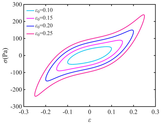
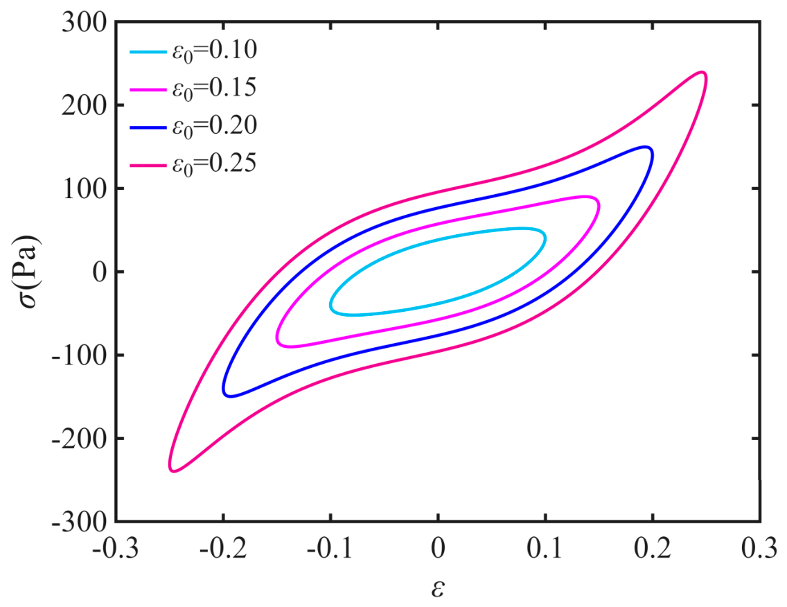
Based on the mechanical coefficients and material-level coefficients, when S = 1 m² and h = 1 m, with k₂ = 1 × 10⁴ N/m³, k₃ = 1 × 10³ N/m, k₄ = 1 × 10² N/m, and c₂ = 12 N·s/m, the corresponding parameters are K₂ = 1 × 10⁴ Pa, K₃ = 1 × 10³ Pa, K₄ = 1 × 10² Pa, and C₂ = 12 Pa·s [47]. Substituting these parameters and ω = 50 into Equation (17) yields the stress–strain curve shown in Figure 17.

Figure 17. Illustrative model-predicted stress–strain hysteresis loops for prescribed material-level parameters at different strain amplitudes.

Using the constitutive relation in Equation (17), the predicted hysteresis loops contain both the fundamental and third-harmonic contributions of the cubic spring. The loops are theoretical examples for the selected material-level parameters. The stress–strain relationship provides a basis for the design of an MRE damper for milling-chatter suppression.

6.2. Stability Analysis of Milling Chatter

With an MNES added to the milling system, vibration only in the y direction is considered, only the radial component of the cutting force is retained, and a zeroth-order approximation is adopted, with the directional coefficient treated as the scalar constant B₀. The governing equations of motion are then given by

$$\left\{\begin{array}{l}{m}_1{\ddot{y}}_1+c_1{\dot{y}}_1+k_1{y}_1+k_2{(y_1-y_2)}^3+k_3(y_1-y_3)=K_{\mathrm{c}}{a}_{\mathrm{p}}{B}_0\left[y_1(t)-y_1(t-T)\right]\\ m_2{\ddot{y}}_2+c_2({\dot{y}}_2-{\dot{y}}_3)+k_4(y_2-y_3)+k_2{(y_2-y_1)}^3=0\\ k_3(y_3-y_1)+c_2({\dot{y}}_3-{\dot{y}}_2)+k_4(y_3-y_2)=0\end{array}\right.$$

(18)

Unlike the prescribed harmonic-excitation model adopted for the frequency-response analysis, Equation (18) explicitly retains the regenerative term K_ca_pB₀[y₁(t) − y₁(t − T)]. This displacement-dependent delay feedback determines the local stability of the cutting process within the adopted linear regenerative-chatter approximation. The stability boundaries are therefore derived from the characteristic roots of the delayed system rather than from the value of the prescribed-force response. The analysis is conditional on the assumed one-direction structural dynamics and the zeroth-order, constant-directional-factor approximation.

At equilibrium, x₁ = x₂ = x₃ = 0, the cubic terms vanish to first order because

$${\displaystyle \frac{\partial }{\partial y_1}}\left[k_2{(y_1-y_2)}^3\right]{|}_0=3k_2{(y_1-y_2)}^2{|}_0=0$$

with similar results for the other partial derivatives. Hence, the cubic stiffness k₂ is absent from the linearized equations. Applying the Laplace transform with Y_i = L{y_i}, s as the Laplace variable, and Λ = K_ca_pB₀, and using L{y₁(t − T)} = e^−STY₁, the linearized system becomes

$$\left\{\begin{array}{l}(m_1{s}^2+c_{1}s+k_1+k_3)Y_1-k_3{Y}_3=\Lambda (1-e^{-sT})Y_1\\ (m_2{s}^2+c_{2}s+k_4)Y_2-(c_{2}s+k_4)Y_3=0\\ -k_3{Y}_1-(c_{2}s+k_4)Y_2+(c_{2}s+k_3+k_4)Y_3=0\end{array}\right.$$

(19)

From the third equation in Equation (19), X₃ can be written as

$$Y_3={\displaystyle \frac{k_3{Y}_1+(c_{2}s+k_4)Y_2}{c_{2}s+k_3+k_4}}$$

(20)

Substituting Equation (20) into the first two equations of Equation (19) and rearranging yields the following homogeneous linear system in X₁ and X₂:

$$\left\{\begin{array}{l}\left[A(s)-\Lambda (1-e^{-sT})(c_{2}s+k_3+k_4)\right]Y_1-k_3(c_{2}s+k_4)Y_2=0\hfill \\ -k_3(c_{2}s+k_4)Y_1+D(s)Y_2=0\hfill \end{array}\right.$$

(21)

where

$$\begin{gathered} A(s)=(m_1{s}^2+c_{1}s+k_1+k_3)(c_{2}s+k_3+k_4)-k_3^2, \\ D(s)=m_2{s}^2(c_{2}s+k_4)+k_3(m_2{s}^2+c_{2}s+k_4). \end{gathered}$$

For a nonzero solution, the determinant of the 2 × 2 system must vanish:

$$\left[A(s)-\Lambda (1-e^{-sT})(c_{2}s+k_3+k_4)\right]D(s)-k_3^2{(c_{2}s+k_4)}^2=0$$

(22)

Define

$$\begin{gathered} H(s)=A(s)D(s)-k_3^2{(c_{2}s+k_4)}^2 \\ R(s)=(c_{2}s+k_3+k_4)D(s) \end{gathered}$$

The characteristic equation can then be expressed in the compact form

$$H(s)=\Lambda (1-e^{-sT})R(s)$$

(23)

Set s = iω, with w > 0 representing the chatter frequency, and let θ = ωT. Write

$$\left\{\begin{array}{l}H(i\omega )=H_{\mathrm{r}}+i{H}_{\mathrm{i}}\hfill \\ R(i\omega )=R_{\mathrm{r}}+i{R}_{\mathrm{i}}\hfill \end{array}\right.$$

(24)

The characteristic equation becomes

$$H_{\mathrm{r}}+i{H}_{\mathrm{i}}=\Lambda (1-e^{-i\theta })(R_{\mathrm{r}}+i{R}_{\mathrm{i}})$$

(25)

Using 1 − e^−iθ = 1 − cosθ + isinθ and separating the real and imaginary parts yields

$$\left\{\begin{array}{c}{H}_{\mathrm{r}}=\Lambda \left[(1-cos\theta )R_{\mathrm{r}}-sin\theta R_{\mathrm{i}}\right]\\ H_{\mathrm{i}}=\Lambda \left[(1-cos\theta )R_{\mathrm{i}}+sin\theta R_{\mathrm{r}}\right]\end{array}\right.$$

(26)

Eliminating Λ from the two equations in Equation (26) gives

$$(H_{\mathrm{i}}{R}_{\mathrm{r}}-H_{\mathrm{r}}{R}_{\mathrm{i}})(1-cos\theta )-(H_{\mathrm{i}}{R}_{\mathrm{i}}+H_{\mathrm{r}}{R}_{\mathrm{r}})sin\theta =0$$

(27)

Define

$$\left\{\begin{array}{c}{E}_1=H_{\mathrm{i}}{R}_{\mathrm{r}}-H_{\mathrm{r}}{R}_{\mathrm{i}}\\ E_2=H_{\mathrm{i}}{R}_{\mathrm{i}}+H_{\mathrm{r}}{R}_{\mathrm{r}}\end{array}\right.$$

(28)

Then

$$E_1(1-cos\theta )=E_{2}sin\theta$$

(29)

Using the half-angle identities, the expression reduces to

$$tan{\displaystyle \frac{\theta }{2}}={\displaystyle \frac{E_2}{E_1}}$$

(30)

Thus,

$$\theta =2\left(arctan{\displaystyle \frac{E_2}{E_1}}+l\pi \right), l=0,1,2,\dots$$

(31)

Taking the magnitudes of both sides of H(iω)= Λ(1 − e^−iθ)R(iω) gives

$$\left|H(i\omega )\right|=K_{\mathrm{c}}{a}_{\mathrm{p}}{B}_0\left|1-e^{-i\theta }\right|\left|R(i\omega )\right|$$

(32)

Hence, the critical depth of cut is given by

$$a_{\mathrm{p}}={\displaystyle \frac{\left|H(i\omega )\right|}{K_{\mathrm{c}}{B}_0\sqrt{2(1-cos\theta )}\left|R(i\omega )\right|}}$$

(33)

The spindle speed is obtained follows from T = θ/ω and n = 60/(NT)

$$n={\displaystyle \frac{60\omega }{N\theta }}$$

(34)

Here, H(iω) and R(iω) are expressed solely in terms of the original system parameters

$$\left\{\begin{array}{l}\begin{array}{ll}H(i\omega )=& \left[(m_1{(i\omega )}^2+i{c}_1\omega +k_1+k_3)(i{c}_2\omega +k_3+k_4)-k_3^2\right]\\ & \times \left[m_2{(i\omega )}^2(i{c}_2\omega +k_4)+k_3(m_2{(i\omega )}^2+i{c}_2\omega +k_4)\right]\\ & -k_3^2{(i{c}_2\omega +k_4)}^2\end{array}\hfill \\ \begin{array}{ll}R(i\omega )=& (i{c}_2\omega +k_3+k_4)\\ & \times \left[m_2{(i\omega )}^2(i{c}_2\omega +k_4)+k_3(m_2{(i\omega )}^2+i{c}_2\omega +k_4)\right]\end{array}\hfill \end{array}\right.$$

(35)

Thus, the expression for ap does not involve intermediate displacement variables x₁, x₂, x₃; it depends only on the physical parameters m₁, c₁, k₁, m₂, c₂, k₃, k₄, the cutting parameters K_c and B₀, the chatter frequency ω, and the tooth-passing period T.

Without the NES, the system simplifies to the classical single-degree-of-freedom milling model

$$m_1{\ddot{y}}_1+c_1{\dot{y}}_1+k_1{y}_1=K_{\mathrm{c}}{a}_{\mathrm{p}}{B}_0\left[y_1(t)-y_1(t-T)\right]$$

(36)

Setting s = iω and θ = ωT gives

$$k_1-m_1{\omega }^2+i{c}_1\omega =K_{\mathrm{c}}{a}_{\mathrm{p}}{B}_0(1-e^{-i\theta })$$

(37)

Separating the real and imaginary parts and then eliminating K_ca_pB₀ gives

$$tan{\displaystyle \frac{\theta }{2}}={\displaystyle \frac{k_1-m_1{\omega }^2}{c_1\omega }}$$

(38)

Therefore, the phase angle θ can be expressed as

$$\theta =2\left[arctan\left({\displaystyle \frac{k_1-m_1{\omega }^2}{c_1\omega }}\right)+l\pi \right], l=0,1,2,\dots$$

(39)

The critical depth of cut is then obtained from the modulus relation

$$a_{\mathrm{p}}={\displaystyle \frac{\sqrt{{(k_1-m_1{\omega }^2)}^2+{(c_1\omega )}^2}}{K_{\mathrm{c}}{B}_0\sqrt{2(1-cos\theta )}}}$$

(40)

The spindle-speed formula is identical to that in Equation (34).

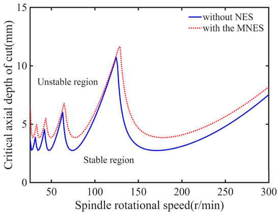
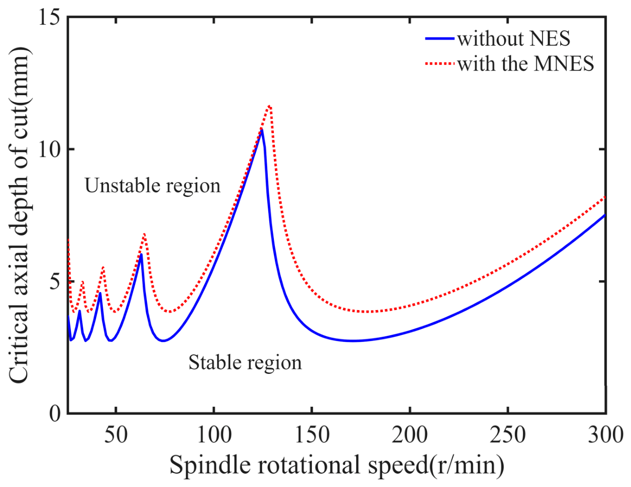
A chatter stability lobe diagram describes milling stability in terms of the relationship between spindle speed and depth of cut. Substituting m₁ = 4 kg, m₂ = 0.4 kg, k₁ =1 × 10⁴ N/m, c₁ = 12 N⋅s/m, c₂ = 12 N⋅s/m, k₃ = 1 × 10³ N/m, k₄ = 1 × 10² N/m, K_c = 1 ×10⁶ N/m², B₀ = 0.5, and the number of teeth N = 4 into Equations (33) and (40) yields the stability lobe diagram shown in Figure 18.

Figure 18. Stability lobe diagram of the milling system.

As shown in Figure 18, the stable milling region is substantially enlarged after the MNES is added. At three representative spindle speeds of n = 50, 100, and 150 r/min, the critical cutting depths increase from 2.87, 5.67, and 3.13 mm without NES to 3.86, 6.13, and 4.68 mm with MNES, respectively, corresponding to increases ranging from 8.11% to 49.52%. In the calculations, the principal phase value was restricted to the range (0, π), and the lobe orders were taken as l = 0, 1, 2, 3, 4, corresponding to the number of full periods experienced by the vibration within the delay time. Each lobe curve was further required to satisfy T > 0, a_p1 > 0, a_p2 > 0, and n > 0, with all quantities being finite; points not meeting these conditions were discarded. These criteria rules ensure that all plotted lobes represent physically admissible stability boundaries.

The first derivative of the cubic nonlinear stiffness vanishes at the equilibrium point; consequently, the conventional linear stability lobe diagram is independent of k₂. The lobe diagram provides linear stability boundaries that must be verified by a more direct approach. Time-domain simulation provides a direct means of verification, in which the original nonlinear delay differential equations are numerically integrated to observe whether the vibration decays or diverges.

Following the same procedure as in Equation (14), Equation (18) can be expressed as the following first-order system:

$$\left\{\begin{array}{l}{\dot{q}}_1=q_2\hfill \\ {\dot{q}}_2={\displaystyle \frac{1}{m_1}}\left\{K_{\mathrm{c}}{a}_{\mathrm{p}}{B}_0\left[q_1(t)-q_1(t-T)\right]-c_1{q}_2-k_1{q}_1-k_3(q_1-q_5)-k_2{(q_1-q_3)}^3\right\}\hfill \\ {\dot{q}}_3=q_4\hfill \\ {\dot{q}}_4={\displaystyle \frac{1}{m_2}}\left[k_3(q_1-q_5)-k_2{(q_3-q_1)}^3\right]\hfill \\ {\dot{q}}_5=q_4-{\displaystyle \frac{1}{c_2}}\left[k_3(q_5-q_1)+k_4(q_5-q_3)\right]\hfill \end{array}\right.$$

(41)

The state equation of the reduced model without NES is expressed as

$$\left\{\begin{array}{l}{\dot{q}}_1=q_2\hfill \\ {\dot{q}}_2={\displaystyle \frac{1}{m_1}}\left\{K_{\mathrm{c}}{a}_{\mathrm{p}}{B}_0\left[q_1(t)-q_1(t-T)\right]-c_1{q}_2-k_1{q}_1\right\}\hfill \end{array}\right.$$

(42)

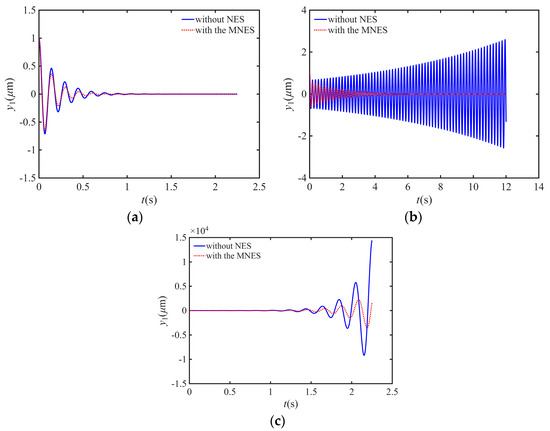
Supplementary time-domain verification was performed using the Runge–Kutta method based on Equations (41) and (42). The selected parameters are m₁ = 4 kg, m₂ = 0.4 kg, k₁ =1 × 10⁴ N/m, c₁ = 12 N⋅s/m, c₂ = 12 N⋅s/m, k₃ = 1 × 10³ N/m, k₄ = 1 × 10² N/m, K_c = 1 × 10⁶ N/m², B₀ = 0.5, and the number of teeth N = 4.

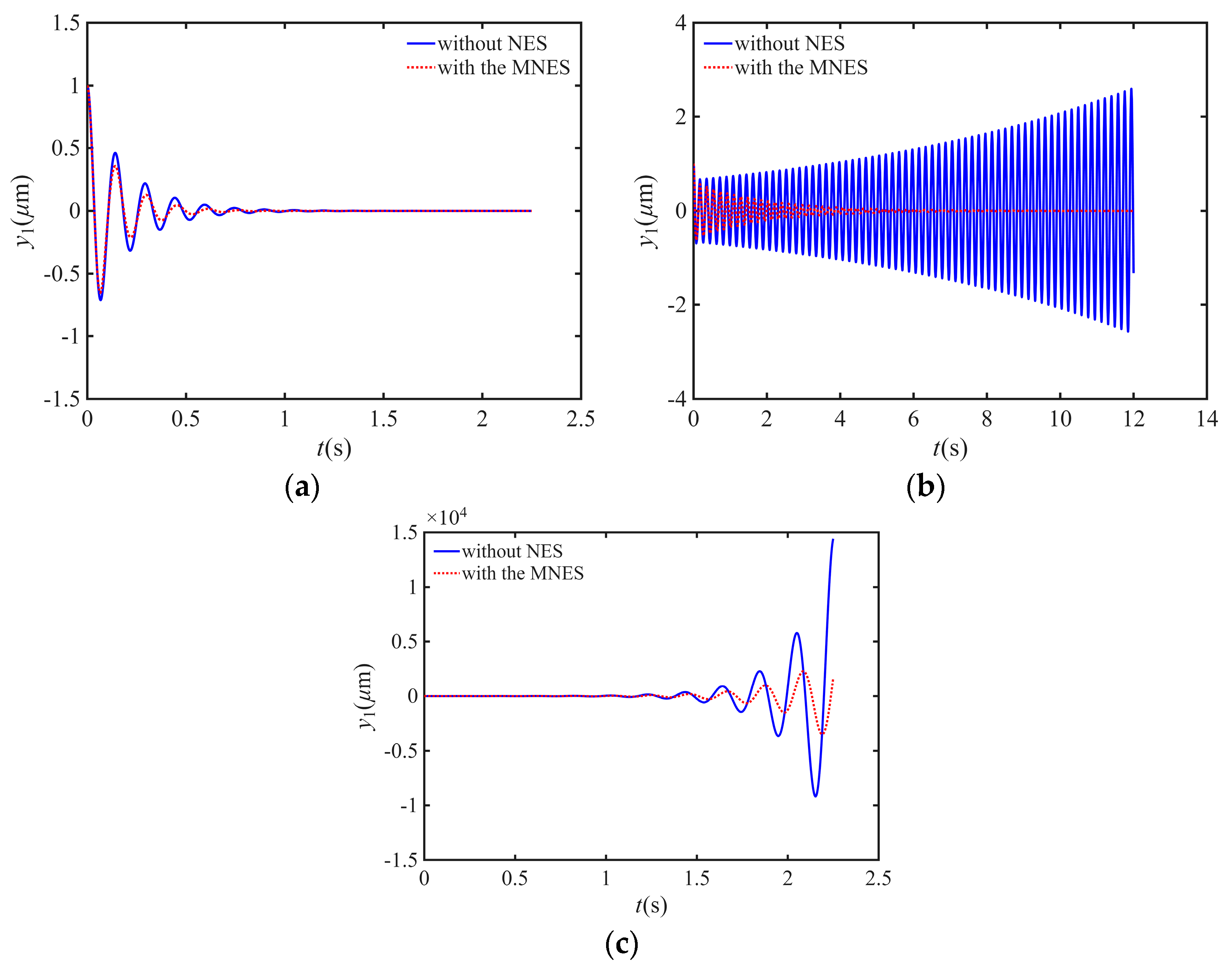
To validate the accuracy of the stability lobe diagram, three representative operating points, specifically (200, 1.5), (200, 3.5), and (200, 5.5), were selected. According to the lobe diagram prediction, these points are located in the stable region, near the critical boundary, and in the unstable region, respectively. Supplementary time-domain simulations were performed for these operating points using the delayed cutting force model incorporating regenerative effects (Equation (18)). Figure 19a shows the time-domain response at the stable point (200, 1.5), where the vibration amplitude decays gradually with time, indicating a stable system. Figure 19c shows the time-domain response at the unstable point (200, 5.5), where the vibration amplitude diverges continuously, indicating the occurrence of chatter. Figure 19b compares the simulated displacement time histories with and without the MNES at the intermediate cutting depth, demonstrating that MNES significantly enlarges the stable cutting region. The time-domain simulation results agree well with the lobe diagram predictions, thereby validating the reliability of the stability analysis method and demonstrating that MNES can effectively suppress milling chatter.

Figure 19. Time history of vibration displacement: (a) n = 200 r/min and a_p = 1.5 mm. (b) n = 200 r/min and a_p = 3.5 mm. (c) n = 200 r/min and a_p = 5.5 mm.

7. Conclusions

In this study, a viscoelastic Kelvin–Voigt element is introduced into a nonlinear energy sink, and a new MRE-based viscoelastic nonlinear energy sink is proposed. Its vibration reduction performance under dynamic cutting forces is investigated. The main-system amplitude-frequency response curves are obtained using the HBM and validated against Runge–Kutta numerical integration in MATLAB. The effects of the system parameters on vibration reduction performance are analyzed. The maximum main-system amplitude is also investigated by simultaneously varying the nonlinear stiffness coefficient and damping ratio for different mass ratios, and the corresponding optimal parameter ranges of the MNES are identified. The main conclusions are as follows.

• The appropriate selection of the nonlinear stiffness coefficient enables the MNES to maintain a robust main-system response under different excitation amplitudes. As the nonlinear stiffness increases, the main-system resonance amplitude first decreases and then increases. For a given nonlinear stiffness and a small damping ratio, the MNES provides slightly better vibration reduction performance than the TNES under the different excitation amplitudes considered.
• Compared with the TNES, the MNES cannot fully exploit the vibration-reduction capability of the viscoelastic material when the linear stiffness ratio α₂ is excessively small or large. As the damping ratio increases, the main-system resonance amplitude first decreases and then increases for both the TNES and the MNES; however, at the same damping ratio, the MNES provides better vibration reduction performance, with a larger reduction in vibration amplitude and a wider vibration-reduction frequency band.
• As the mass ratio increases, the maximum main-system amplitude initially decreases and then remains nearly unchanged, while the optimal ranges of the nonlinear stiffness coefficient and damping ratio broaden. However, an excessively large mass ratio increases the additional mass of the system. Therefore, a moderate mass ratio combined with appropriate values of the other parameters is required to achieve favorable MNES vibration reduction performance.
• Based on the proposed parametric model, simulations are performed to determine parameter values that provide favorable vibration-damping performance. The results provide guidance for fabricating MREs with effective vibration-damping characteristics. Moreover, the MNES was incorporated into the milling system, and the corresponding stability lobe diagram was plotted. To verify the accuracy of the stability lobe diagram, supplementary time-domain simulations were conducted at representative operating points. The results show that the vibration decays gradually at the stable point and diverges at the unstable point, consistent with the lobe diagram predictions, thereby validating the reliability of the stability analysis.

In summary, the appropriate selection of MNES parameters can yield better vibration reduction performance than the TNES. These findings provide a theoretical basis for potential practical applications of MNES to chatter suppression in milling.

References

- Zheng, Y.; Zhao, Z.; Li, H.; Xu, S.; Xu, J. A novel approach for accurate in-situ chatter detection by iterative Vold-Kalman and LMS adaptive filtering of milling signals. Mech. Syst. Signal Process. 2025, 225, 112291. [Google Scholar] [CrossRef] [Scilit]
- Sun, L.; Huang, X.; Jiang, Z.; Zhao, J.; Wang, X. Multi-source heterogeneous sensor information fusion framework for intelligent online chatter detection in different milling conditions. Knowl.-Based Syst. 2025, 330, 114488. [Google Scholar] [CrossRef] [Scilit]
- Li, Z.; Song, Q.; Jin, P.; Liu, Z.; Wang, B.; Ma, H. Chatter suppression techniques in milling processes: A state of the art review. Chin. J. Aeronaut. 2024, 37, 1–23. [Google Scholar] [CrossRef] [Scilit]
- Munoa, J.; Beudaert, X.; Dombovari, Z.; Altintas, Y.; Budak, E.; Brecher, C.; Stepan, G. Chatter suppression techniques in metal cutting. CIRP Ann. 2016, 65, 785–808. [Google Scholar] [CrossRef] [Scilit]
- Li, X.; Ni, J.; Liu, X.; Yue, C.; Yang, S.; Ji, X.; Liang, S.Y.; Wang, L. Chatter-free milling of aerospace thin-walled parts. J. Mater. Process. Technol. 2025, 341, 118903. [Google Scholar] [CrossRef] [Scilit]
- Ma, S.; Xiao, J.; Liu, H.; Liu, S.; Tian, Y. Modeling and analysis for time-varying dynamics of thin-walled workpieces in mirror milling considering material removal. Sci. China Technol. Sci. 2023, 66, 1883–1898. [Google Scholar] [CrossRef] [Scilit]
- Chao, L.; Jun, Z.; Hui, T.; Wanhua, Z. Timely Chatter Detecting Method in Milling with Integrated Energy Ratio and Amplitude Standard Deviation of Vibration Signal. J. Mech. Eng. 2024, 60, 11–23. [Google Scholar] [CrossRef] [Scilit]
- Liu, B.; Liu, C.; Yu, X.; Zhou, Y.; Wang, D. Prediction, detection, and suppression of regenerative chatter in milling. Adv. Mech. Eng. 2022, 14, 168781322211297. [Google Scholar] [CrossRef] [Scilit]
- Zhu, L.; Liu, C. Recent progress of chatter prediction, detection and suppression in milling. Mech. Syst. Signal Process. 2020, 143, 106840. [Google Scholar] [CrossRef] [Scilit]
- Altintas, Y.; Stepan, G.; Budak, E.; Schmitz, T.; Kilic, Z.M. Chatter Stability of Machining Operations. J. Manuf. Sci. Eng. 2020, 142, 110801. [Google Scholar] [CrossRef] [Scilit]
- Celikag, H.; Ozturk, E.; Sims, N.D. Can mode coupling chatter happen in milling? Int. J. Mach. Tool. Manu. 2021, 165, 103738. [Google Scholar] [CrossRef] [Scilit]
- Du, Y.; Liang, Z.; Gao, Z.; Chen, S.; Yue, Y.; Zhang, J.; Liu, H.; Zheng, H.; Liu, B.; Qiu, T.; et al. Investigation on the dominant mechanism of chatter in high-load robot milling process based on theoretical and experimental analysis. J. Sound Vib. 2025, 600, 118886. [Google Scholar] [CrossRef] [Scilit]
- Xin, S.; Tang, X.; Wu, J.; Peng, F.; Yan, R.; Yang, W. Investigation of the low-frequency chatter in robotic milling. Int. J. Mach. Tools Manuf. 2023, 190, 104048. [Google Scholar] [CrossRef] [Scilit]
- Li, N.; Zhao, J.; Sun, R.; Cui, L.; Wang, X. A review on cutting chatter detection and suppression in robotic milling. Robot. Comput.-Integr. Manuf. 2026, 100, 103219. [Google Scholar] [CrossRef] [Scilit]
- Mladjenovic, C.; Marinković, D.; Monkova, K.; Knežev, M.; Živković, A. A Novel Mathematical Model for Predicting Self-Excited Vibrations in Micromilling of Aluminium 7075. Metals 2025, 15, 1375. [Google Scholar] [CrossRef] [Scilit]
- Franco, O.; Beudaert, X.; Erkorkmaz, K.; Munoa, J. Feed Drive Control and Non-Linear Friction Interaction Effect on Machining Chatter Stability Prediction. J. Manuf. Mater. Process. 2024, 8, 207. [Google Scholar] [CrossRef] [Scilit]
- Wang, M.; Qin, P.; Zan, T.; Gao, X.; Han, B.; Zhang, Y. Improving optimal chatter control of slender cutting tool through more accurate tuned mass damper modeling. J. Sound Vib. 2021, 513, 116393. [Google Scholar] [CrossRef] [Scilit]
- Bolsunovsky, S.; Vermel, V.; Gubanov, G.; Leontiev, A. Reduction of Flexible Workpiece Vibrations with Dynamic Support Realized as Tuned Mass Damper. Procedia CIRP 2013, 8, 230–234. [Google Scholar] [CrossRef] [Scilit]
- Yang, Y.; Xie, R.; Liu, Q. Design of a passive damper with tunable stiffness and its application in thin-walled part milling. Int. J. Adv. Manu. Technol. 2017, 89, 2713–2720. [Google Scholar] [CrossRef] [Scilit]
- Dong, X.; Li, X.; Zhang, L.; Zhao, F.; Li, Y.; Yang, Y. Chatter suppression analysis for variable pitch cutter in milling. Int. J. Adv. Manuf. Tech. 2024, 131, 3193–3203. [Google Scholar] [CrossRef] [Scilit]
- Wan, M.; Dang, X.-B.; Zhang, W.-H.; Yang, Y. Chatter suppression in the milling process of the weakly-rigid workpiece through a moving fixture. J. Mater. Process. Technol. 2022, 299, 117293. [Google Scholar] [CrossRef] [Scilit]
- Cui, G.; Zhou, J.; Xu, J.-H.; Xu, Y.-P.; Zeng, L. Active control of forced vibration in spindle milling with integrated electromagnetic actuator %J Journal of Vibration Engineering. J. Vib. Eng. 2024, 37, 1803–1810. [Google Scholar] [CrossRef]
- Wang, C.; Zhang, X.; Liu, J.; Cao, H.; Chen, X. Adaptive vibration reshaping based milling chatter suppression. Int. J. Mach. Tools Manuf. 2019, 141, 30–35. [Google Scholar] [CrossRef] [Scilit]
- Li, D.; Cao, H.; Chen, X. Fuzzy control of milling chatter with piezoelectric actuators embedded to the tool holder. Mech. Syst. Signal Process. 2021, 148, 107190. [Google Scholar] [CrossRef] [Scilit]
- Wan, S.; Li, X.; Su, W.; Yuan, J.; Hong, J. Active chatter suppression for milling process with sliding mode control and electromagnetic actuator. Mech. Syst. Signal Process. 2020, 136, 106528. [Google Scholar] [CrossRef] [Scilit]
- Nguyen, V.; Johnson, J.; Melkote, S. Active vibration suppression in robotic milling using optimal control. Int. J. Mach. Tools Manuf. 2020, 152, 103541. [Google Scholar] [CrossRef] [Scilit]
- Long, X.; Jiang, H.; Meng, G. Active vibration control for peripheral milling processes. J. Mater. Process. Technol. 2013, 213, 660–670. [Google Scholar] [CrossRef] [Scilit]
- Rashid, A.; Nicolescu, C.M. Design and implementation of tuned viscoelastic dampers for vibration control in milling. Int. J. Mach. Tools Manuf. 2008, 48, 1036–1053. [Google Scholar] [CrossRef] [Scilit]
- Oladapo, B.I.; Muhammad, M.A.; Adebiyi, V.A.; Oluwole, B.; Usman, H. Model hybrid magnetorheological damping prediction in machine tools. Eng. Struct. 2020, 213, 110621. [Google Scholar] [CrossRef] [Scilit]
- Jaafar, M.F.; Mustapha, F.; Mustapha, M. Review of current research progress related to magnetorheological elastomer material. J. Mater. Res. Technol. 2021, 15, 5010–5045. [Google Scholar] [CrossRef] [Scilit]
- Zhu, J.-T.; Xu, Z.-D.; Guo, Y.-Q. Experimental and Modeling Study on Magnetorheological Elastomers with Different Matrices. J. Mater. Civ. Eng. 2013, 25, 1762–1771. [Google Scholar] [CrossRef] [Scilit]
- Xu, Z.-D.; Chen, Z.-H.; Huang, X.-H.; Zhou, C.-Y.; Hu, Z.-W.; Yang, Q.-H.; Gai, P.-P. Recent Advances in Multi-Dimensional Vibration Mitigation Materials and Devices. Front. Mater. 2019, 6, 143. [Google Scholar] [CrossRef] [Scilit]
- Tian, Y.; Xu, Z.-D.; Guo, Y.-Q.; Zhu, L.-H.; Dong, Y.-R.; Li, Q.-Q.; Hu, Z.-W.; Wei, Y.-X. Experimental and theoretical investigation on magnetorheological elastomers containing carbonyl iron particles coated with silane coupling agent. Smart Mater. Struct. 2024, 33, 065028. [Google Scholar] [CrossRef] [Scilit]
- Shuaishuai, S.; Jian, Y.; Tanju, Y.; Haiping, D.; Gursel, A.; Shiwu, Z.; Weihua, L. Development of a nonlinear adaptive absorber based on magnetorheological elastomer. J. Intel. Mat. Syst. Str. 2018, 29, 194–204. [Google Scholar] [CrossRef] [Scilit]
- Komatsuzaki, T.; Inoue, T.; Iwata, Y. Experimental Investigation of an Adaptively Tuned Dynamic Absorber Incorporating Magnetorheological Elastomer with Self-Sensing Property. Exp. Mech. 2016, 56, 871–880. [Google Scholar] [CrossRef] [Scilit]
- Chen, C.; Peng, F.; Yan, R.; Tang, X.; Li, Y.; Fan, Z. Rapid prediction of posture-dependent FRF of the tool tip in robotic milling. Robot. Comput.-Integr. Manuf. 2020, 64, 101906. [Google Scholar] [CrossRef] [Scilit]
- Cui, G.; Li, B.; Tian, W.; Liao, W.; Zhao, W. Dynamic modeling and vibration prediction of an industrial robot in manufacturing. Appl. Math. Model. 2022, 105, 114–136. [Google Scholar] [CrossRef] [Scilit]
- Yuan, L.; Sun, S.; Pan, Z.; Ding, D.; Gienke, O.; Li, W. Mode coupling chatter suppression for robotic machining using semi-active magnetorheological elastomers absorber. Mech. Syst. Signal Process. 2019, 117, 221–237. [Google Scholar] [CrossRef] [Scilit]
- Liu, P.; Li, B.; Zhao, W.; Cui, G.; Tian, W.; Liao, W. Design and experimental study of a magnetorheological elastomer vibration absorber for chatter suppression in robotic milling. J. Vib. Eng. 2025, 38, 1699–1710. [Google Scholar] [CrossRef]
- Zhao, W.; Li, B.; Tian, W.; Liu, P.; Liao, W. Magnetorheological elastomer absorber-based chatter suppression in robotic milling. Robot. Comput.-Integr. Manuf. 2024, 88, 102740. [Google Scholar] [CrossRef] [Scilit]
- Qingyan, Y.; Weihua, L. Theoretical analysis and experiment of magneto rheological elastomer vibration absorber for milling thin-walled workpiece. Mech. Sci. Technol. Aerosp. Eng. 2022, 41, 263–269. [Google Scholar] [CrossRef]
- Norouzi, M.; Sajjadi Alehashem, S.M.; Vatandoost, H.; Ni, Y.Q.; Shahmardan, M.M. A new approach for modeling of magnetorheological elastomers. J. Intel. Mat. Syst. Str. 2016, 27, 1121–1135. [Google Scholar] [CrossRef] [Scilit]
- Hemmatian, M.; Sedaghati, R.; Rakheja, S. Characterization and modeling of temperature effect on the shear mode properties of magnetorheological elastomers. Smart Mater. Struct. 2020, 29, 115001. [Google Scholar] [CrossRef] [Scilit]
- Wang, Q.; Dong, X.; Li, L.; Ou, J. A nonlinear model of magnetorheological elastomer with wide amplitude range and variable frequencies. Smart Mater. Struct. 2017, 26, 065010. [Google Scholar] [CrossRef] [Scilit]
- Song, Q.; Ai, X.; Tang, W. Prediction of simultaneous dynamic stability limit of time–variable parameters system in thin-walled workpiece high-speed milling processes. Int. J. Adv. Manuf. Tech. 2011, 55, 883–889. [Google Scholar] [CrossRef] [Scilit]
- Geng, X.-F.; Ding, H. Theoretical and experimental study of an enhanced nonlinear energy sink. Nonlinear Dyn. 2021, 104, 3269–3291. [Google Scholar] [CrossRef] [Scilit]
- Li, W.H.; Zhou, Y.; Tian, T.F. Viscoelastic properties of MR elastomers under harmonic loading. Rheol. Acta 2010, 49, 733–740. [Google Scholar] [CrossRef] [Scilit]
Disclaimer/Publisher’s Note: The statements, opinions and data contained in all publications are solely those of the individual author(s) and contributor(s) and not of MDPI and/or the editor(s). MDPI and/or the editor(s) disclaim responsibility for any injury to people or property resulting from any ideas, methods, instructions or products referred to in the content. |
© 2026 by the authors. Licensee MDPI, Basel, Switzerland. This article is an open access article distributed under the terms and conditions of the Creative Commons Attribution (CC BY) license.