Reliability Analysis of Tuned Mass Damper-Equipped Structures Under Stochastic Excitation

Abstract

Tuned mass dampers (TMDs) are commonly used to reduce excessive vibrations in engineering structures. Although their vibration control performance has been widely studied, the reliability of TMD-equipped structures under stochastic excitations has not been sufficiently investigated. In practical applications, random loads and system uncertainties may significantly affect structural safety, and an efficient evaluation of failure probability remains a challenging task. Thus, the applications of these methods are greatly limited in vibration control. In this work, the structural reliability of systems equipped with TMDs is analyzed by adopting the first-passage time (FPT) as the failure criterion. Numerical investigations are performed on continuous beam models with TMDs under different types of stochastic excitation. In addition, an experimental study on a two-story steel frame structure is conducted to further examine the reliability performance of TMD-controlled systems. To reduce the computational cost associated with Monte Carlo simulation, a data-driven classification method is employed to approximate the failure domain based on a limited number of samples. The results indicate that the proposed approach enables accurate reliability estimation with a substantial reduction in computational cost, making it suitable for large-scale reliability analysis of vibration-controlled structures under stochastic excitation. The experimental results further demonstrate the applicability of the proposed reliability assessment method for practical vibration control problems.

1. Introduction

Structural vibrations caused by environmental and operational loads are common in many engineering structures. These vibrations can lead to serviceability issues, fatigue damage, and reduced structural safety during long-term operation. Such problems are frequently observed in civil and mechanical systems subjected to wind, traffic loads, or machinery-induced excitations. To reduce unwanted vibrations, many control and mitigation techniques have been developed, including passive, semi-active, and active solutions. Among these approaches, tuned mass dampers (TMDs) are widely used because of their simple design, passive nature, and stable performance. Therefore, TMDs have been applied in a variety of structures, such as buildings, bridges, towers, and other systems that are sensitive to vibration [1,2].

Many studies on structures equipped with tuned mass dampers have focused on deterministic dynamic response analysis. Previous work has mainly examined issues such as tuning methods, parameter sensitivity, and vibration reduction under harmonic or transient excitations [3,4]. In practical applications, the vibration control performance of TMD-equipped structures is influenced by various sources of uncertainty. These uncertainties may arise from variations in material properties, modeling assumptions, and installation conditions, as well as from randomness in external loads such as wind, traffic, or operational excitations [5,6]. Even when a TMD is properly designed based on nominal parameters, its actual performance may deviate from the expected response due to these uncertain factors. Under such conditions, uncertainties in external loading and system parameters can have a noticeable effect on the structural response and overall performance. As a result, the effectiveness of TMDs cannot always be fully assessed using deterministic analysis alone. This has motivated increasing attention toward probabilistic and reliability-based approaches for evaluating the vibration response of structures with TMDs under uncertain loading conditions.

Structural reliability analysis provides a probabilistic framework to quantify the influence of uncertainty on structural safety [7,8]. For vibration-related problems, failure is commonly defined by response thresholds, and the first-passage time (FPT) has been widely used to characterize the occurrence of failure events in stochastic dynamic systems. Compared with conventional response measures, the FPT offers a direct and physically meaningful indicator for reliability assessment under random excitation [9,10].

Despite its importance, the reliability analysis of TMD-controlled structures under stochastic excitation remains limited. The evaluation of FPT distributions and failure probabilities generally relies on Monte Carlo simulation, which requires a large number of dynamic analyses. This is particularly relevant for engineering applications where repeated high-fidelity simulations are computationally prohibitive [11,12].

In addition to computational challenges, the reliability analysis of TMD-equipped structures is further complicated when continuous systems and experimental structures are considered [13,14]. For continuous structural models, such as beams, the dynamic response is governed by partial differential equations, and the interaction between the primary structure and the TMD may involve multiple vibration modes. This increases the complexity of stochastic response analysis and leads to a higher computational cost in reliability evaluation.

From an experimental perspective, reliability analysis under stochastic excitation is even more demanding [15,16]. Repeated tests are required to capture the variability of structural response, and the definition of failure events based on first-passage criteria must account for measurement noise and experimental uncertainties. As a result, experimental studies on the reliability performance of TMD-controlled structures remain limited, and most existing works focus primarily on deterministic or mean-response-based assessments.

In recent years, data-driven methods have been introduced to improve the efficiency of reliability analysis [17,18,19]. Classification techniques can be used to approximate failure regions and reduce the number of required simulations. However, their application to vibration control problems involving tuned mass dampers (TMDs) remains limited. In particular, the combined consideration of TMD dynamics, FPT-based reliability indicators, and experimental validation has not been sufficiently explored. In practical engineering applications, these aspects are often critical. For example, uncertainties in excitation characteristics and system parameters can significantly affect the estimated first-passage reliability of TMD-controlled structures, while the lack of experimental verification may limit the applicability of data-driven models in real operating environments.

In large-scale engineering systems operating under long-term and variable conditions, the need for efficient and reliability-oriented analysis methods becomes more pronounced. Large inter-basin water transfer infrastructures, such as the eastern route of the South-to-North Water Diversion Project, involve complex structural and mechanical components that are continuously subjected to stochastic excitations and operational uncertainties. National research initiatives on multi-source water allocation and intelligent water conveyance further emphasize the importance of developing computationally efficient tools to support safety assessment and intelligent operation of such large-scale systems.

Despite extensive studies on tuned mass dampers, most existing works focus on deterministic response analysis or optimal parameter tuning. Studies addressing the stochastic reliability of TMD-equipped structures remain relatively limited, particularly those combining first-passage-time-based reliability, data-driven methods, and experimental validation [20,21,22]. Moreover, the influence of uncertainty in both structural parameters and stochastic excitation on reliability performance has not been sufficiently investigated in an integrated framework. Recent studies have also emphasized the importance of stochastic and reliability-based design of TMD systems [23,24,25,26]. For instance, time-dependent effects in wind-induced vibrations have been highlighted, as well as probabilistic optimization strategies for TMD parameters under stochastic loading conditions.

Motivated by these observations, this study presents a reliability assessment approach for TMD-equipped structures subjected to stochastic excitation. The proposed approach integrates stochastic dynamic analysis, FPT-based failure characterization, and data-driven classification to achieve an efficient estimation of failure probability. Both numerical models and experimental tests are considered to demonstrate the applicability of the method.

The main contributions of this study are summarized as follows:

• The reliability performance of structures equipped with TMDs is investigated under stochastic excitation using the first-passage time as the failure criterion.
• The effects of random loading characteristics and system uncertainties on the FPT distribution and failure probability are examined through numerical and experimental studies.
• A data-driven classification method is employed to improve the efficiency of reliability analysis while maintaining sufficient accuracy.
• Experimental validation on a two-story steel frame structure is conducted to demonstrate the practical applicability of the proposed approach.

The remainder of this paper is organized as follows. Section 2 presents the stochastic dynamic analysis of a beam equipped with a TMD. Section 3 extends the analysis to transversal vibration. Section 4 describes the experimental reliability investigation of a two-story steel frame structure. Finally, the conclusions are drawn in Section 5.

2. Longitudinal Vibration of a Beam with a TMD

The longitudinal vibration model of a cantilever beam with a tuned mass damper gives a simple but useful way to study its dynamic behavior and reliability. In this model, the beam moves only along its length, not sideways. This simplifies the analysis and helps build clear equations for vibration and uncertainty studies. The model is used to check how well the TMD can reduce vibration when the beam is under random forces.

It also has real engineering meaning for tall and slender structures, such as towers, antenna masts, and support columns.

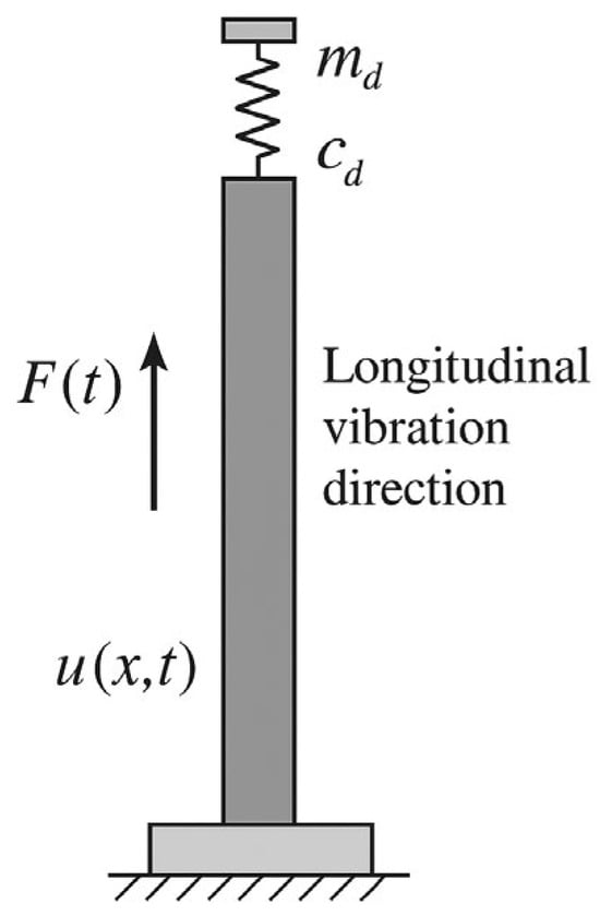
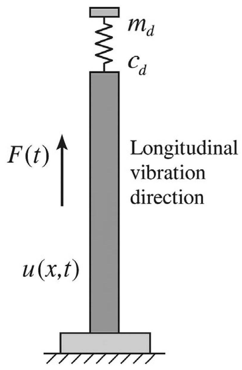
As shown in Figure 1, the beam is placed vertically and is fixed at the bottom. A tuned mass damper is attached to the free end of the beam. The external excitation force f(x, t) acts along the beam axis. This causes the beam to vibrate in the longitudinal direction.

Figure 1. Schematic representation of the longitudinal vibration of a beam with a TMD.

The beam is treated as a continuous system. The displacement along the beam is written as u(x, t), where x is the coordinate along the beam length and t is time. The governing equation of motion can be expressed as

$$EA{\displaystyle \frac{{\mathsf{\partial }}^{2}u(x,t)}{\mathsf{\partial }{x}^2}}=\rho A{\displaystyle \frac{{\mathsf{\partial }}^{2}u(x,t)}{\mathsf{\partial }{t}^2}}-f(x,t)$$

(1)

where ρ is the material density, E is Young’s modulus, and A is the cross-sectional area of the beam.

2.1. Dynamic Analysis of Longitudinal Vibrations in a Beam with a TMD

In the present formulation, the beam is assumed to behave as a linear elastic system subjected to stochastic excitation. The material properties and geometric parameters are considered spatially uniform, and damping is introduced through the TMD system. The transition from the continuous formulation to the reduced-order model is achieved using the Rayleigh–Ritz method, where the displacement field is approximated by a finite set of admissible trial functions.

To describe the longitudinal dynamic behavior of the beam equipped with a TMD, the following analytical formulation is introduced. The displacement field for each frequency can be expressed as

$$\mu (x,t)={\displaystyle \sum _{i=1}^n{\lambda }_i}(t){\psi }_i(x)$$

(2)

where i = 1, 2, …, n indexes the number of terms in the approximation; λi(t) is the Ritz coefficient, capturing the time-dependent component of the mode shape; and ψi(x) is the trial function, representing the spatial component of the mode shape.

At the bottom end (x = 0), the beam is fixed, and the displacement is zero. At the top end (x = L), the beam interacts with the TMD. The boundary condition is given by:

$$EA{\displaystyle \frac{\mathsf{\partial }\mu (L,t)}{\mathsf{\partial }x}}=-k\mu (L,t)-c{\displaystyle \frac{\mathsf{\partial }\mu (L,t)}{\mathsf{\partial }t}}-m{\displaystyle \frac{{\mathsf{\partial }}^2\mu (L,t)}{\mathsf{\partial }{t}^2}}$$

(3)

where k, c, and m are the stiffness, damping, and mass of the TMD, respectively.

This boundary condition balances the internal axial force in the beam with the reactive forces introduced by the TMD, thereby governing the system’s dynamic response at the free end.

2.1.1. Strain Energy of the System

The total strain energy is calculated as:

$$V_{\mathrm{spring}}$$

(4)

where the strain energy of the beam and the spring are given by:

$$V_{\mathrm{beam}}={\displaystyle \frac{1}{2}}{\displaystyle {\int }_0^{L}E}A{\left({\displaystyle \frac{\mathsf{\partial }\mu }{\mathsf{\partial }x}}\right)}^{2}dx,\hspace{1em}{V}_{\mathrm{spring}}={\displaystyle \frac{1}{2}}{k}_t{\mu }^2(x,t){|}_{x=L}$$

(5)

• $V_{\mathrm{beam}}$: strain energy stored in the beam
• $V_{\mathrm{spring}}$: strain energy stored in the TMD spring

Substituting the displacement approximation:

$$\mu (x,t)={\displaystyle \sum _{i=1}^n{\lambda }_i}(t){\psi }_i(x)$$

(6)

we get:

$$V={\displaystyle \frac{1}{2}}{\displaystyle {\int }_0^{L}E}A{\left({\displaystyle \sum _{i=1}^n{\lambda }_i}{\psi }_i^{\prime }(x)\right)}^{2}dx+{\displaystyle \frac{1}{2}}{k}_t{\left({\displaystyle \sum _{i=1}^n{\lambda }_i}{\psi }_i(L)\right)}^2$$

(7)

Expanding in matrix form:

$$V={\displaystyle \frac{1}{2}}{\overrightarrow{\lambda }}^T\left({\displaystyle {\int }_0^{L}E}A{\psi }_i^{\prime }(x){\psi }_j^{\prime }(x)dx+k_t{\psi }_i(L){\psi }_j(L)\right)\overrightarrow{\lambda }$$

(8)

or more compactly:

$$V={\displaystyle \frac{1}{2}}{\overrightarrow{\lambda }}^T[K]\overrightarrow{\lambda }$$

(9)

where the stiffness matrix [K] is defined as:

$$K_{ij}={\displaystyle {\int }_0^{L}E}A{\psi }_i^{\prime }(x){\psi }_j^{\prime }(x)dx+k_t{\psi }_i(L){\psi }_j(L)$$

(10)

2.1.2. Kinetic Energy of the System

The total kinetic energy of the system is expressed as:

$$T=T_{\mathrm{beam}}+T_{\mathrm{mass}}$$

(11)

where $T_{\mathrm{beam}}$ is kinetic energy of the beam, $T_{\mathrm{mass}}$ is kinetic energy of the TMD mass.

$$T_{\mathrm{beam}}={\displaystyle \frac{1}{2}}{\displaystyle {\int }_0^L\rho }A{\left({\displaystyle \frac{\mathsf{\partial }\mu }{\mathsf{\partial }t}}\right)}^{2}dx,\hspace{1em}{T}_{\mathrm{mass}}={\displaystyle \frac{1}{2}}{m}_t{\left({\displaystyle \frac{\mathsf{\partial }\mu }{\mathsf{\partial }t}}(L,t)\right)}^2$$

(12)

Using the series expansion for displacement:

$$\mu (x,t)={\displaystyle \sum _{i=1}^n{\lambda }_i}(t){\psi }_i(x)$$

(13)

the kinetic energy becomes:

$$T={\displaystyle \frac{1}{2}}{\displaystyle {\int }_0^L\rho }A{\left({\displaystyle \sum _{i=1}^n{\lambda }_i}{\psi }_i(x)\right)}^{2}dx+{\displaystyle \frac{1}{2}}{m}_t{\left({\displaystyle \sum _{i=1}^n{\lambda }_i}{\psi }_i(L)\right)}^2$$

(14)

Expanding the terms, we have:

$$T={\displaystyle \frac{1}{2}}{\displaystyle \sum _{i=1}^n{\displaystyle \sum _{j=1}^n{\lambda }_i}}{\lambda }_j\left({\displaystyle {\int }_0^L\rho }A{\psi }_i(x){\psi }_j(x)dx+m_t{\psi }_i(L){\psi }_j(L)\right)$$

(15)

In matrix form, the kinetic energy is:

$$T={\displaystyle \frac{1}{2}}{\overrightarrow{\lambda }}^T[M]\overrightarrow{\lambda }$$

(16)

where the mass matrix [M] is defined as:

$$M_{ij}={\displaystyle {\int }_0^L\rho }A{\psi }_i(x){\psi }_j(x)dx+m_t{\psi }_i(L){\psi }_j(L)$$

(17)

2.1.3. Rayleigh’s Quotient

The natural frequencies of the system can be determined using Rayleigh’s quotient:

$$R={\omega }^2={\displaystyle \frac{V_{\max }}{T_{\max }}}={\displaystyle \frac{N}{D}}$$

(18)

where N is the maximum strain energy, D is the maximum kinetic energy, and ω is the natural frequency. Rayleigh’s quotient can be expressed as a function of the Ritz coefficients:

$$R=R({\lambda }_1,{\lambda }_2,\dots ,{\lambda }_n)$$

(19)

To find the minimum of R, the partial derivative with respect to each Ritz coefficient is set to zero:

$${\displaystyle \frac{\mathsf{\partial }R}{\mathsf{\partial }{\lambda }_i}}=0\hspace{1em}\mathrm{for}\hspace{1em}i=1,2,\dots ,n$$

(20)

2.1.4. Eigenvalue Problem

Using the strain energy and kinetic energy expressions:

$$N={\displaystyle \frac{1}{2}}{\overrightarrow{\lambda }}^T[K]\overrightarrow{\lambda },\hspace{1em}D={\displaystyle \frac{1}{2}}{\overrightarrow{\lambda }}^T[M]\overrightarrow{\lambda }$$

(21)

Rayleigh’s quotient leads to the generalized eigenvalue problem:

$$([K]-{\mathrm{\Lambda }}^{(n)}[M])\overrightarrow{\lambda }=\overrightarrow{0}$$

(22)

For nontrivial solutions $\overrightarrow{\lambda }\ne \overrightarrow{0}$, the determinant must vanish:

$$\left|[K]-{\mathrm{\Lambda }}^{(n)}[M]\right|=0$$

(23)

The roots of this equation provide the natural frequencies:

$${\omega }_i=\sqrt{{\mathrm{\Lambda }}_i^{(n)}},\hspace{1em}i=1,2,\dots ,n$$

(24)

The eigenvectors $\overrightarrow{\lambda }$ satisfy:

$$([K]-{\mathrm{\Lambda }}_i^{(n)}[M]){\overrightarrow{\lambda }}^{(i)}=\overrightarrow{0}$$

(25)

The corresponding mode shape is:

$${\mu }^{(i)}(x)={\displaystyle \sum _{j=1}^n{\lambda }_j^{(i)}}{\psi }_j(x)$$

(26)

The trial functions ψi(x) for the mode shape expansion are chosen as:

$${\psi }_i(x)=1-\cos \left({\displaystyle \frac{(2i-1)\pi x}{2L}}\right),\hspace{1em}i=1,2,\dots ,n$$

(27)

which meet the beam’s boundary conditions and serve as a practical basis for approximating the mode shapes.

2.1.5. Dynamic Response of the System

The total dynamic response is given by:

$$Y(x,t)={\displaystyle \sum _{i=1}^n{\mu }^{(i)}}(x){\eta }_i(t)$$

(28)

where ${\eta }_i(t)$ are time-dependent generalized coordinates. The governing equation of motion is:

$$EA{\displaystyle \frac{{\mathsf{\partial }}^{2}Y(x,t)}{\mathsf{\partial }{x}^2}}+f(x,t)=\rho A{\displaystyle \frac{{\mathsf{\partial }}^{2}Y(x,t)}{\mathsf{\partial }{t}^2}}$$

(29)

Substituting the mode shape expansion:

$${\displaystyle \sum _{i=1}^n\left[EA\frac{d^2{\mu }^{(i)}(x)}{d{x}^2}\right]}{\eta }_i(t)+f(x,t)=\rho A{\displaystyle \sum _{i=1}^n{\mu }^{(i)}}(x){\displaystyle \frac{d^2{\eta }_i(t)}{{dt}^2}}$$

(30)

The modal form is:

$${\displaystyle \frac{d^2{\eta }_i(t)}{d{t}^2}}+{\omega }_i^2{\eta }_i(t)=Q_i(t)$$

(31)

where $Q_i(t)={\displaystyle {\int }_0^L{\mu }^{(i)}}(x)f(x,t)dx$ is the generalized force.

2.1.6. Solution Using the Laplace Transform

Applying the Laplace transform:

$$L\{{\eta }_i(t)\}={\overline{\eta }}_i(s),\hspace{1em}L\{Q_i(t)\}={\overline{Q}}_i(s)$$

(32)

The second derivative transforms as:

$$L\{{\ddot{\eta }}_i(t)\}{=s}^2{\overline{\eta }}_i(s)-s{\eta }_i(0)-{\dot{\eta }}_i(0)$$

(33)

Substituting into the modal equation:

$${\overline{\eta }}_i(s)={\displaystyle \frac{{\overline{Q}}_i(s)+s{\eta }_i(0)+{\dot{\eta }}_i(0)}{\mathrm{\Delta }}},\hspace{1em}\mathrm{\Delta }=s^2+{\omega }_i^2$$

(34)

Taking the inverse Laplace transform:

$${\eta }_i(t)={\displaystyle {\int }_0^t{Q}_i}(\tau )h(t-\tau )d\tau +g(t){\eta }_i(0)+h(t){\dot{\eta }}_i(0)$$

(35)

where:

$$\begin{array}{c}{Q}_i(\tau )={\displaystyle {\int }_0^L{\mu }^{(i)}}(x)f(x,\tau )dx,\hfill \\ h(t)={\displaystyle \frac{\sin ({\omega }_{i}t)}{{\omega }_i}},\hfill \\ g(t)=\cos ({\omega }_{i}t),\hfill \\ {\displaystyle {\int }_0^t{Q}_i}(\tau )h(t-\tau )d\tau \hfill \end{array}$$

For initial conditions ${\eta }_i(0)=0$ and ${\dot{\eta }}_i(0)=0$, the response simplifies to:

$${\eta }_i(t)={\displaystyle {\int }_0^t{Q}_i}(\tau )h(t-\tau )d\tau$$

(36)

The complete system response is:

$$Y(x,t)={\displaystyle \sum _{i=1}^n{\mu }^{(i)}}(x)\left[{\displaystyle {\int }_0^t{Q}_i}(\tau )h(t-\tau )d\tau \right]$$

(37)

The next step involves performing numerical simulations to study how parametric uncertainties, such as changes in material properties or geometry, affect the structural dynamics of the beam–TMD system. These simulations are essential for assessing the system’s robustness and reliability in practical operating scenarios. The following sections present numerical examples, reliability evaluations using sampling techniques, and Monte Carlo simulations to calculate the probability of structural failure.

2.2. Numerical Study and Benchmarks

2.2.1. Numerical Example of Parameter Uncertainty on Structural Dynamics

The base structure’s properties are modeled with uncertainties as normal distributions. The standard deviations of these properties are shown in Table 1. Sample data are generated using these distributions. Table 1 lists the statistical properties of important structural parameters like elastic modulus, density, and cross-sectional area. These parameters affect the structure’s dynamic response under seismic loading. Including these uncertainties gives a more realistic view of the structure’s performance. Material properties follow normal distributions based on typical engineering tolerances. Coefficients of variation are selected according to reliability studies [27,28].

Table 1. Nominal values and standard deviations of the structural parameters (longitudinal analysis).

Variables	Mean	Standard Deviation
Elastic Modulus ($E$)	2 × 1011	3.6 × 104
Density ($\rho$)	7800	650
Cross-Sectional Area ($A$)	3.14 × 10−4	3.14 × 10−5

Here, the mean value of elastic modulus $E$ is 2 × 10¹¹. The standard deviation is 3.6 × 10⁴. This parameter shows the stiffness of the material. The small standard deviation compared to the mean indicates the material properties are consistent. The mean density is 7800, with a standard deviation of 650. The standard deviation is about 8.3% of the mean, showing moderate variation due to uneven material distribution or manufacturing issues. The mean cross-sectional area is 3.14 × 10⁻⁴. The standard deviation is 3.14 × 10⁻⁵. This parameter affects stiffness and load-bearing ability. The standard deviation is 10% of the mean. This reflects possible geometric differences during fabrication.

We assume that the seismic model has a natural frequency of 25.224 rad/s and a damping ratio of 0.4. The power spectral density (PSD) of the white noise input is 0.031 m²/s³. The failure condition is defined as a displacement greater than 0.028 m.

2.2.2. Feature Importance Using Random Forest Regression

Random Forest regression is used to find feature importance scores. This helps identify the factors that affect structural reliability the most. The analysis also shows less important features, which can be removed to save computation time while keeping accuracy. The results, based on a sample size of N = 4000, are shown in Table 2.

Table 2. Feature Importance for Increased Standard Deviation of Elastic Modulus (N = 4000).

Feature	Importance
Density ($\rho$)	0.54881
Cross-Sectional Area ($A$)	0.35985
Elastic Modulus ($E$)	0.09133

Table 2 shows the updated feature importance scores. We can see that the density (ρ) remained the most important factor with its importance slightly decreasing to 0.54881. The decrease is relative to the initial feature importance ranking before modifying the standard deviation of (E). The cross-sectional area (A) decreased to 0.35985 but still had a significant effect. On the other hand, the elastic modulus (E) became less important with a score of 0.09133.

2.2.3. Reliability Analysis Using Latin Hypercube Sampling and MCS

The reliability of the beam with a TMD under dynamic loading was studied using Latin hypercube sampling (LHS). LHS is a method that samples inputs to cover the input distributions well, ensuring accurate failure probability estimates.

Monte Carlo simulation was used to calculate the failure probability. This involved running many iterations of the system model with samples generated by LHS. The failure condition was set as a displacement greater than 0.028 m, which is the maximum allowed deformation for structural safety. The LHS sample size is 20,000, the number of Monte Carlo simulations is 10,000. The convergence criterion is based on stabilization of failure probability.

2.2.4. Performance Comparison of Machine Learning Models

The dataset used for training the machine learning models is generated using Latin hypercube sampling, ensuring a uniform coverage of the input parameter space. The dataset is divided into training and testing subsets to evaluate model generalization. The neural network model consists of multiple fully connected layers with nonlinear activation functions, while ensemble models such as Random Forest and XGBoost are configured with standard hyperparameters to ensure fair comparison.

Several machine learning models were trained to predict failure probability. Their performance was evaluated using root mean square error, mean absolute error, and relative error, and the results are presented in Table 3. Material properties follow normal distributions based on typical engineering tolerances. Coefficients of variation are selected according to reliability studies [27,28].

Table 3. Performance comparison of machine learning models for failure probability estimation.

Model	RMSE	MAE	Relative Error (%)
Random Forest	0.030384	0.021408	9.16
Gradient Boosting	0.027676	0.020013	10.70
XGBoost	0.030734	0.021780	9.22
Neural Network	0.025835	0.018020	1.17

The neural network model performed the best, with the lowest RMSE, MAE, and relative error. This shows that it is better at capturing complex relationships in the reliability analysis of the beam with a TMD.

2.2.5. Scatter Plots of Predictions

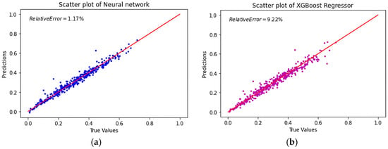
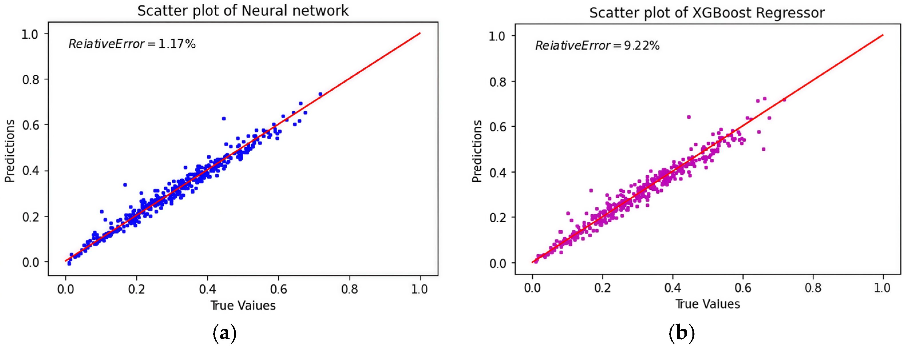
Figure 2 shows scatter plots comparing the predicted and true values for the neural network and XGBoost models. These plots show how accurately each model predicts failure probability. The red line shows the ideal case where the predicted values match the true values exactly.

Figure 2. The performance of machine learning models was compared. (a) Test vs. predicted values (neural network); (b) test vs. predicted values (XGBoost).

As shown in Figure 2a. The neural network model’s predictions are close to the red line, therefore it could realize high accuracy. The relative error is only 1.17%. The NN model handles complex input–output relationships well. However, there are some outliers, which might be due to difficult input areas or insufficient training data.

In contrast, the scatter plot for the XGBoost model in Figure 2b shows a broader spread around the red line, reflecting higher variability and a relative error of 9.22%. The higher number and larger magnitude of outliers suggest that XGBoost struggles to fully capture the complex dependencies in the data. This leads to less consistent predictions. These results show that XGBoost is less effective at handling highly non-linear relationships compared to the neural network. Its performance could be improved with better hyperparameter tuning or alternative feature engineering methods.

The results show that machine learning techniques are effective for predicting structural failures under dynamic conditions with uncertain parameters. Among the models tested, the neural network performed the best. It achieved the lowest RMSE, MAE, and relative error. This highlights the strength of neural networks in capturing the nonlinear and interdependent relationships in the reliability analysis of mechanical systems with TMDs.

3. Transversal Vibration with a TMD

Compared with longitudinal vibration, transversal vibration introduces additional complexity due to the coupling between shear deformation and bending effects. This leads to a different dynamic behavior and a more complex uncertainty propagation mechanism, which justifies the separate analysis presented in this section.

In fact, transversal vibrations are more complex than longitudinal ones because they involve shear and bending. These vibrations cause bending and sideways movement. Therefore, studying transversal vibrations is important. It helps us understand how the beam behaves under real conditions.

3.1. Transversal Shear and Bending Effects in Beam Dynamics

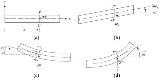
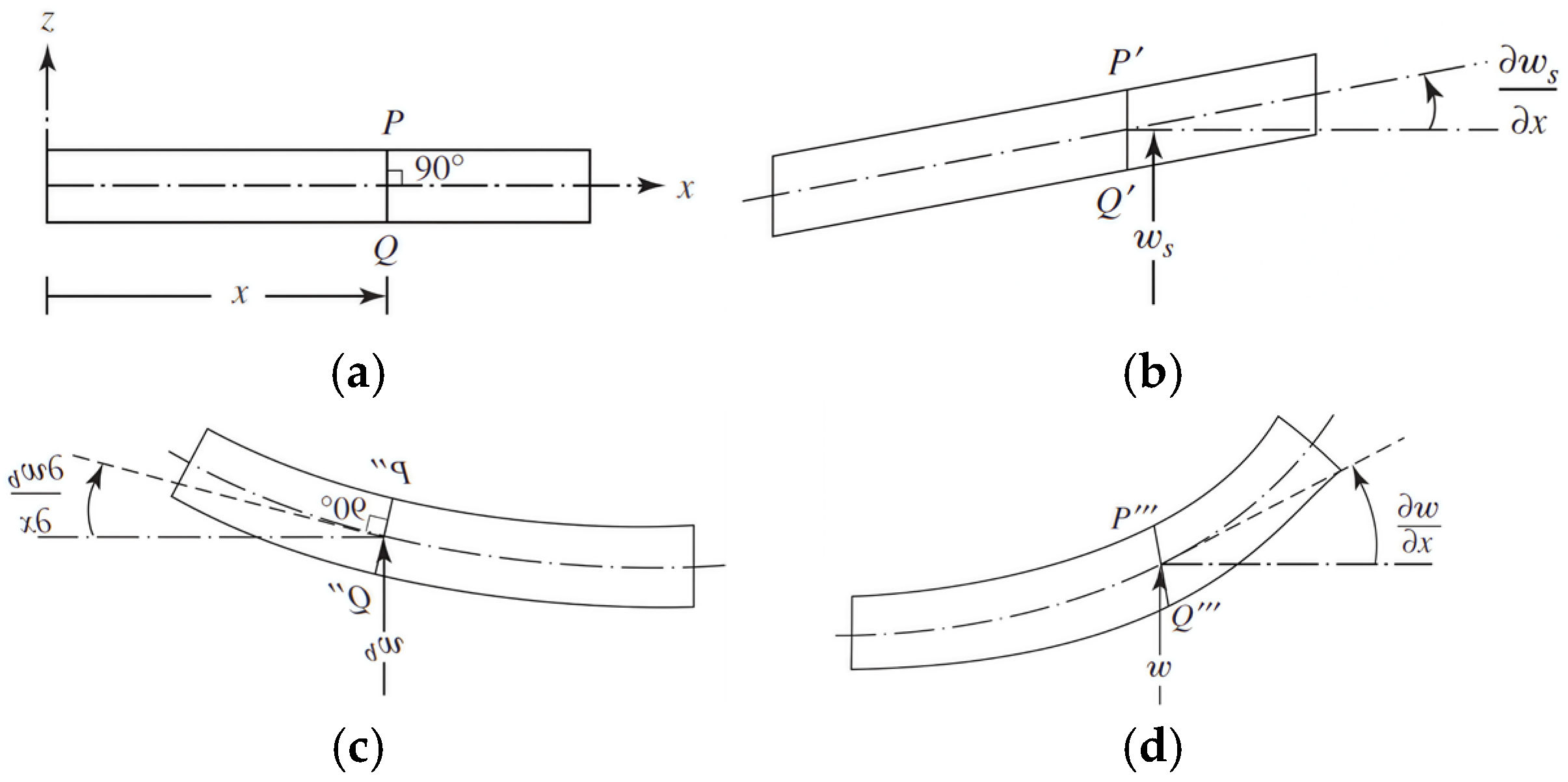
Transversal vibrations are different from longitudinal vibrations. They involve both shear and bending, which affect the beam’s behavior. Figure 3 shows the different deformation modes a beam can experience: (a) no deformation, (b) shear deformation only, (c) bending deformation only, and (d) total deformation.

Figure 3. Modes of bending and shear deformations in a beam. (a) No deformation; (b) shear deformation only; (c) bending deformation only; (d) total deformation.

The total transverse displacement of the beam’s centerline is given as:

$$w=w_s+w_b$$

(38)

where $w_s$ represents shear deformation, and $w_b$ represents bending deformation.

The total slope of the beam can be written as:

$${\displaystyle \frac{\mathsf{\partial }w}{\mathsf{\partial }x}}={\displaystyle \frac{\mathsf{\partial }{w}_s}{\mathsf{\partial }x}}+{\displaystyle \frac{\mathsf{\partial }{w}_b}{\mathsf{\partial }x}}$$

(39)

In this equation:

• $w_s$ is the part of displacement caused by shear.
• $w_b$ is the part of displacement caused by bending.
• ${\displaystyle \frac{\mathsf{\partial }{w}_b}{\mathsf{\partial }x}}$ shows the rotation of the cross-section.
• ${\displaystyle \frac{\mathsf{\partial }{w}_s}{\mathsf{\partial }x}}$ shows the shear angle.

The total slope combines the effects of both shear and bending deformation along the beam. In many cases, the bending slope is assumed to be negligible (${\displaystyle \frac{\mathsf{\partial }{w}_b}{\mathsf{\partial }x}}=0$).

Under this assumption:

$${\displaystyle \frac{\mathsf{\partial }w}{\mathsf{\partial }x}}={\displaystyle \frac{\mathsf{\partial }{w}_s}{\mathsf{\partial }x}}$$

(40)

This assumption simplifies the equation of motion as:

$$kGA{\displaystyle \frac{{\mathsf{\partial }}^{2}w(x,t)}{\mathsf{\partial }{x}^2}}+f=\rho A{\displaystyle \frac{{\mathsf{\partial }}^{2}w(x,t)}{\mathsf{\partial }{t}^2}}$$

(41)

where:

• k is the shear correction factor.
• G is the shear modulus of the material.
• A is the cross-sectional area.
• ρ is the material density.
• f is the external force applied.

The term $kGA{\displaystyle \frac{{\mathsf{\partial }}^{2}w}{\mathsf{\partial }{x}^2}}$ is the restoring force from shear deformation. It depends on the material and size of the beam. The term $\rho A{\displaystyle \frac{{\mathsf{\partial }}^{2}w}{\mathsf{\partial }{t}^2}}$ is the inertia from dynamic forces. This equation shows how the beam stays balanced under transverse forces.

3.2. Analytical Analysis of Transversal Vibration

The horizontal displacement function for each mode is expressed as:

$$X(x,t)={\displaystyle \sum _{i=1}^n{\lambda }_i}(t){\psi }_i(x)$$

(42)

where ${\lambda }_i(t)$ represents the time-dependent Ritz coefficient, and ${\psi }_i(x)$ represents the spatial trial function.

The trial functions are defined as:

$${\psi }_i(x)=1-\cos \left({\displaystyle \frac{(2i-1)\pi x}{2L}}\right),\hspace{1em}i=1,2,\dots ,n$$

(43)

ensuring that boundary conditions are satisfied. The cosine term captures the oscillatory behavior typical of vibration modes, maintaining zero displacement at the fixed end.

The boundary conditions for the beam are:

$$\left\{\begin{array}{ll}X(0,t)=0\hfill & (\mathrm{fixed} \mathrm{end} \mathrm{at} x=0)\hfill \\ kGA{\displaystyle \frac{\mathsf{\partial }X(L,t)}{\mathsf{\partial }x}}=-k_{t}X(L,t)-c_t{\displaystyle \frac{\mathsf{\partial }X(L,t)}{\mathsf{\partial }t}}-m_t{\displaystyle \frac{{\mathsf{\partial }}^{2}X(L,t)}{\mathsf{\partial }{t}^2}}\hfill & (\mathrm{free} \mathrm{end} \mathrm{with} \mathrm{TMD} \mathrm{at} x=L),\hfill \end{array}\right.$$

(44)

The first condition means no movement at the fixed end. The second condition shows how the TMD interacts with the beam at the free end; it includes the shear force, spring force (kt), damping force (ct), and inertia (mt).

3.2.1. Strain Energy of the System

The strain energy V includes contributions from both the beam and the spring element of the TMD:

$$V=V_{\mathrm{beam}}+V_{\mathrm{spring}}$$

(45)

The strain energy in the beam is:

$$V_{\mathrm{beam}}={\displaystyle \frac{1}{2}}{\displaystyle {\int }_0^{L}k}GA{\left({\displaystyle \frac{\mathsf{\partial }X}{\mathsf{\partial }x}}\right)}^{2}dx$$

(46)

where G is the shear modulus, A is the cross-sectional area, and k is the shear correction factor. This term represents the energy due to shear deformation.

The strain energy in the TMD spring is:

$$V_{\mathrm{spring}}={\displaystyle \frac{1}{2}}{k}_t{X}^2(L,t)$$

(47)

where kt is the TMD spring constant, and X(L, t) is the displacement at the free end.

Substituting the displacement function X(x, t) into the strain energy expressions:

$$V={\displaystyle \frac{1}{2}}{\displaystyle {\int }_0^{L}k}GA{\left({\displaystyle \sum _{i=1}^n{\lambda }_i}{{\psi }^{\prime }}_i(x)\right)}^{2}dx+{\displaystyle \frac{1}{2}}{k}_t{\left({\displaystyle \sum _{i=1}^n{\lambda }_i}{\psi }_i(L)\right)}^2$$

(48)

In matrix form:

$$V={\displaystyle \frac{1}{2}}\left[\begin{array}{cccc}{\lambda }_1& {\lambda }_2& \cdots & {\lambda }_n\end{array}\right][K]\left[\begin{array}{c}{\lambda }_1\\ {\lambda }_2\\ ⋮\\ {\lambda }_n\end{array}\right]$$

(49)

where [K] is the stiffness matrix:

$$K_{ij}={\displaystyle {\int }_0^{L}k}GA{{\psi }^{\prime }}_i(x){{\psi }^{\prime }}_j(x)dx+k_t{\psi }_i(L){\psi }_j(L)$$

(50)

The stiffness matrix [K] combines the material properties of the beam with the influence of the TMD, capturing the system’s overall resistance to deformation.

3.2.2. Kinetic Energy of the System

The kinetic energy T of the system includes contributions from the beam and the TMD mass:

$$T=T_{\mathrm{beam}}+T_{\mathrm{mass}}$$

(51)

The kinetic energy of the beam is:

$$T_{\mathrm{beam}}={\displaystyle \frac{1}{2}}{\displaystyle {\int }_0^L\rho }A{\left({\displaystyle \frac{\mathsf{\partial }X}{\mathsf{\partial }t}}\right)}^{2}dx$$

(52)

where ρ is the material density, and A is the cross-sectional area. This term captures the motion of the beam. The kinetic energy of the TMD mass is:

$$T_{\mathrm{mass}}={\displaystyle \frac{1}{2}}{m}_t{\left({\displaystyle \frac{\mathsf{\partial }X}{\mathsf{\partial }t}}(L,t)\right)}^2$$

(53)

where mt is the mass of the TMD, and ${\displaystyle \frac{\mathsf{\partial }X}{\mathsf{\partial }t}}(L,t)$ is the velocity at the free end.

Substituting the displacement function X(x, t):

$$T={\displaystyle \frac{1}{2}}{\displaystyle {\int }_0^L\rho }A{\left({\displaystyle \sum _{i=1}^n{\lambda }_i}{\psi }_i(x)\right)}^{2}dx+{\displaystyle \frac{1}{2}}{m}_t{\left({\displaystyle \sum _{i=1}^n{\lambda }_i}{\psi }_i(L)\right)}^2$$

(54)

In matrix form:

$$T={\displaystyle \frac{1}{2}}\left[\begin{array}{cccc}{\lambda }_1& {\lambda }_2& \cdots & {\lambda }_n\end{array}\right][M]\left[\begin{array}{c}{\lambda }_1\\ {\lambda }_2\\ ⋮\\ {\lambda }_n\end{array}\right]$$

(55)

where the mass matrix [M] is:

$$M_{ij}={\displaystyle {\int }_0^L\rho }A{\psi }_i(x){\psi }_j(x)dx+m_t{\psi }_i(L){\psi }_j(L)$$

(56)

The matrix [M] reflects the mass distribution along the beam and the contribution from the TMD.

3.2.3. Rayleigh Quotient and Natural Frequencies

The Rayleigh quotient R estimates the natural frequencies of the system:

$$R={\omega }^2={\displaystyle \frac{N}{D}}={\displaystyle \frac{V_{\max }}{T_{\max }}}$$

(57)

where:

• N is the maximum strain energy.
• D is the maximum kinetic energy.
• ω is the natural frequency.

Expressed using Ritz coefficients:

$$R=R({\lambda }_1,{\lambda }_2,\dots ,{\lambda }_n)$$

(58)

Minimizing R with respect to λi:

$${\displaystyle \frac{\mathsf{\partial }R}{\mathsf{\partial }{\lambda }_i}}=0,\hspace{1em}i=1,2,\dots ,n$$

(59)

3.2.4. Eigenvalue Problem

The strain and kinetic energies in terms of [K] and [M]:

$$N={\displaystyle \frac{1}{2}}{\overrightarrow{\lambda }}^T[K]\overrightarrow{\lambda },\hspace{1em}D={\displaystyle \frac{1}{2}}{\overrightarrow{\lambda }}^T[M]\overrightarrow{\lambda }$$

(60)

Substituting into the Rayleigh quotient leads to:

$${\displaystyle \frac{\mathsf{\partial }}{\mathsf{\partial }{\lambda }_i}}\left({\displaystyle \frac{{\overrightarrow{\lambda }}^T[K]\overrightarrow{\lambda }}{{\overrightarrow{\lambda }}^T[M]\overrightarrow{\lambda }}}\right)=0$$

(61)

Rewriting yields the eigenvalue problem:

$$\left([K]-{\mathrm{\Lambda }}^{(n)}[M]\right)\overrightarrow{\lambda }=\overrightarrow{0}$$

(62)

For nontrivial solutions:

$$\det \left([K]-{\mathrm{\Lambda }}^{(n)}[M]\right)=0$$

(63)

The eigenvalues ${\mathrm{\Lambda }}_i^{(n)}$ correspond to squared natural frequencies:

$${\omega }_i=\sqrt{{\mathrm{\Lambda }}_i^{(n)}},\hspace{1em}i=1,2,\dots ,n$$

(64)

The eigenvectors $\overrightarrow{\lambda }$ define the mode shapes.

3.2.5. Mode Shapes and Dynamic Response

Once the eigenvalues ${\mathrm{\Lambda }}_i^{(n)}$ are determined, the corresponding mode shapes ${\overrightarrow{\lambda }}^{(i)}$ are obtained by solving:

$$\left([K]-{\mathrm{\Lambda }}_i^{(n)}[M]\right){\overrightarrow{\lambda }}^{(i)}=\overrightarrow{0}$$

(65)

Each mode shape represents a unique spatial deformation pattern of the beam, associated with a specific natural frequency. These mode shapes reveal the dynamic deformation behavior of the structure during vibration.

The dynamic response of the system is expressed as:

$$Y(x,t)={\displaystyle \sum _{i=1}^n{X}^{(i)}}(x){\eta }_i(t)$$

(66)

where:

• $X^{(i)}$ is the spatial mode shape for the i-th mode.
• ${\eta }_i(t)$ is the generalized coordinate describing the time-dependent amplitude of the i-th mode.

The equation of motion for each mode is:

$${\ddot{\eta }}_i(t)+{\omega }_i^2{\eta }_i(t)=Q_i(t)$$

(67)

where $Q_i(t)$ is the generalized force acting on the i-th mode:

$$Q_i(t)={\displaystyle {\int }_0^L{X}^{(i)}}(x)f(x,t)dx$$

(68)

This equation shows how the amplitude ${\eta }_i(t)$ changes over time for each mode. It accounts for the effect of the external force f(x, t). It explains how natural frequencies and external inputs affect the beam’s vibrations.

3.2.6. Solution of the Equation of Motion

The solution to the equation of motion incorporates convolution integrals, also known as Duhamel’s integral, to account for the effects of external forces over time. The dynamic response of the system is expressed as:

$$Y(x,t)={\displaystyle \sum _{i=1}^n{X}^{(i)}}(x)\left[{\displaystyle {\int }_0^t{Q}_i}(\tau )h_i(t-\tau )d\tau \right]$$

(69)

where:

• $X^{(i)}(x)$ is the mode shape for the i-th mode.
• $Q_i(\tau )$ is the generalized force for the i-th mode at time τ.
• $h_i(t)$ is the impulse response function for the i-th mode.

The impulse response function hi(t) is given by:

$$h_i(t)={\displaystyle \frac{\sin ({\omega }_{i}t)}{{\omega }_i}}$$

(70)

This function characterizes the system’s reaction to an instantaneous force. The convolution integral represents the cumulative effect of the applied force over time. Together, they provide a complete description of the dynamic response of the beam–TMD system under external loading.

3.3. Numerical Study and Benchmarks

3.3.1. Numerical Example of Parameter Uncertainty on Structural Dynamics

The uncertainties in the properties of the base structure are modeled as normal distributions, with the standard deviations listed in Table 4.

Table 4. Nominal values and uncertainties of structural parameters (transversal vibration).

Variables	Mean	Standard Deviation
Shear Modulus (G)	52.5 GPa	5 GPa
Density (ρ)	7800 kg/m3	650 kg/m3
Cross-Sectional Area (A)	3.14 × 10−2 m2	3.14 × 10−3 m2

3.3.2. Feature Importance Using Random Forest Regression

Random Forest regression was used to check which features matter most for predicting failure probability. As shown in Table 5, The cross-sectional area (A) is the most important factor. Density (ρ) and shear modulus (G) are also significant.

Table 5. Feature importance for failure prediction (N = 20,000).

Feature	Importance
Cross-Sectional Area (A)	0.34138
Density (ρ)	0.33700
Shear Modulus (G)	0.32162

Transversal vibration involves higher model complexity. It exhibits higher variability and nonlinear interactions, requiring larger sample size to ensure statistical convergence and more robust feature importance estimation.

3.3.3. Performance Comparison of Models for Failure Probability

To study the reliability of the transverse vibration beam with a TMD under dynamic loading, several machine learning models were trained on datasets of transversal vibrations. The performance metrics for these models are shown in Table 6.

Table 6. Performance of machine learning models for failure probability prediction (N = 20,000).

Model	RMSE	MAE	Relative Error (%)
Random Forest	0.011775	0.009263	1.86
Gradient Boosting	0.011284	0.008923	1.79
XGBoost	0.011541	0.009100	1.82
Neural Network	0.009261	0.007001	0.20

Table 6 provides a comparison for a larger dataset (N = 20,000). The models generally exhibited improved performance with the larger dataset, which can be attributed to better representation of the underlying probabilistic distribution of the input parameters. The neural network model, having the lowest relative error (0.02%), RMSE(0.009261), and MAE(0.007001), shows better performance than other models. XGBoost and Random Forest also benefited from the increased dataset size, with reductions in RMSE and MAE.

3.3.4. Distribution of Predicted Failure Probability

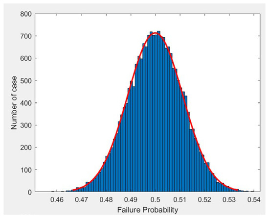
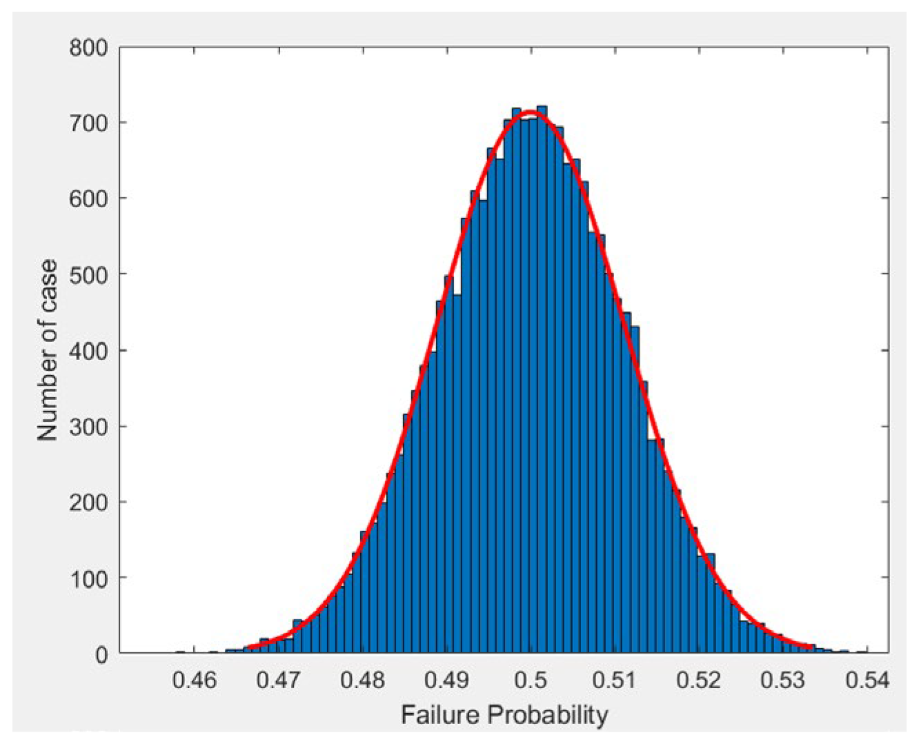
Figure 4 shows the distribution of predicted failure probabilities for a sample size of N = 20,000. We can see that the failure probability follows a normal distribution.

Figure 4. Distribution of predicted failure probability for beam structure (N = 20,000).

Figure 4 shows the distribution of predicted failure probabilities. The mean is about 0.5. Most values are in a small range. This means failure behavior is consistent under the given loading. The red curve is a fitted normal distribution. It matches the histogram well. This shows the variability is symmetric around the mean.

3.3.5. Scatter Plots of Predictions

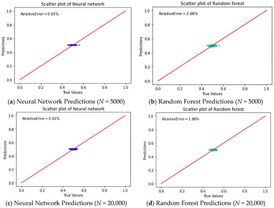
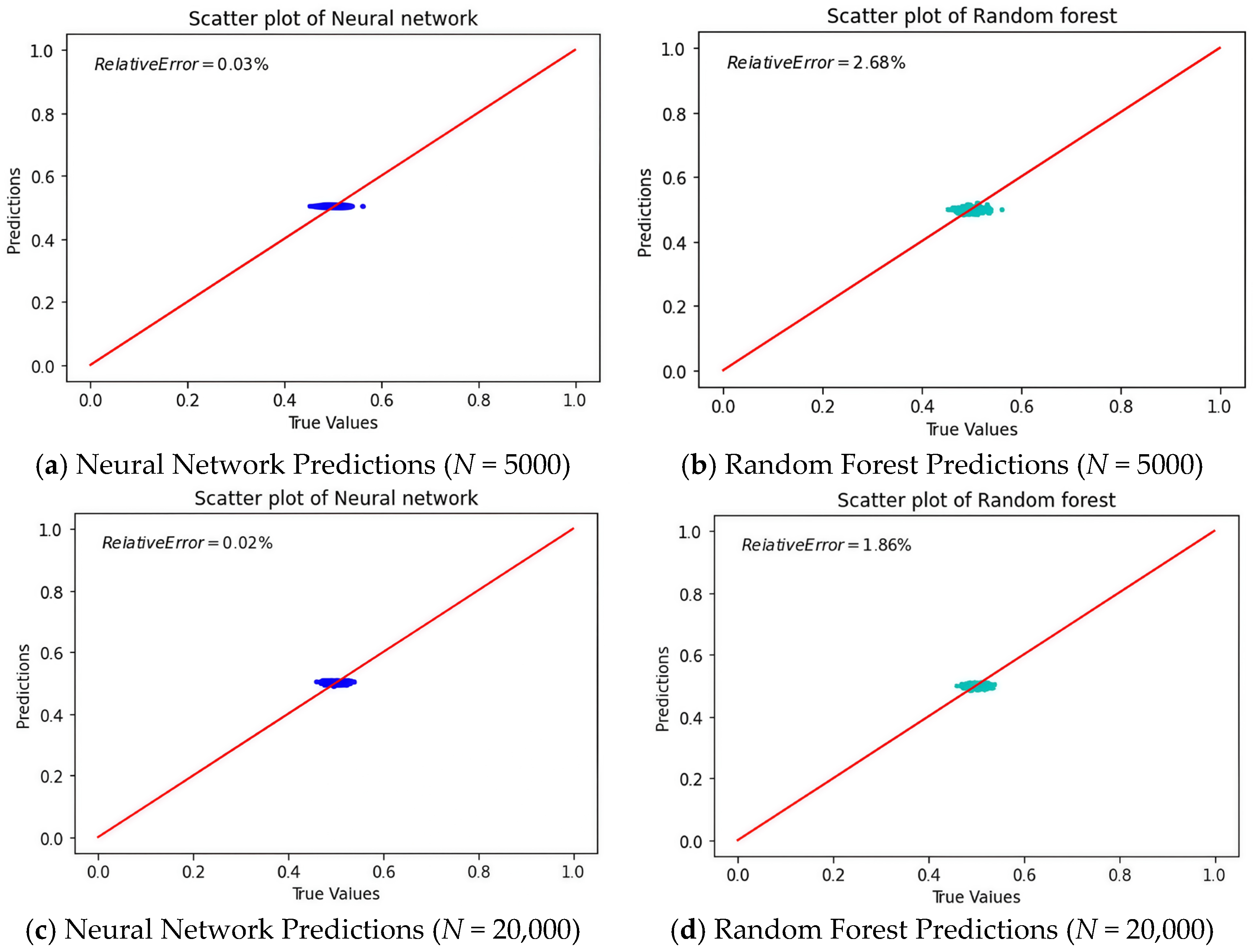
Figure 5 shows a graphical comparison of predicted versus true values for the neural network and Random Forest models with different dataset sizes.

Figure 5. Comparison between predicted and true failure probabilities for different machine learning models. The horizontal axis represents the reference values obtained from Monte Carlo simulations, while the vertical axis shows the predicted values. The red line indicates the ideal agreement between prediction and reference. Results are shown for different dataset sizes to illustrate the influence of training data on model performance.

The scatter plots in Figure 5 show how well the machine learning models predict failure probability. Figure 5a,c show the neural network model’s predictions for datasets with sizes N = 5000 and N = 20,000, respectively. For the neural network model, the data points are close to the reference line, especially for the larger dataset (N = 20,000), indicating high accuracy. The relative error is 0.02% for N = 20,000, confirming that the model performs better with more data.

Figure 5b,d show how the Random Forest model performs. The accuracy gets better with more data. The relative error drops from 2.68% to 1.86%. But the scatter plots show more spread around the reference line than the neural network model. This means Random Forest gives good predictions but may not handle complex patterns as well as the neural network.

In brief, the neural network model performs better than the Random Forest in prediction accuracy, especially with larger datasets. However, the Random Forest is still a good choice because it provides a balance between interpretability and robustness.

In this section, we transitioned from discrete to continuous modeling of dynamic systems, emphasizing the increased complexity and accuracy needed to represent real-world structures. The Rayleigh–Ritz method effectively approximated the behavior of continuous systems, converting partial differential equations into a more manageable form. The analysis of longitudinal and transverse vibrations showed that incorporating tuned mass dampers significantly improved the dynamic response by reducing resonance effects. Using Latin hypercube sampling and Monte Carlo simulation, we assessed the reliability of beam structures with TMDs, considering the stochastic nature of loading and material properties. Additionally, machine learning models like Random Forest and neural networks helped predict failure probabilities and provided insights into factors affecting structural reliability.

4. Experimental Reliability Analysis of the Steel Frame Structure Stochastic Conditions

Real-world structural systems are often exposed to stochastic and dynamic loads, making their behavior inherently complex and challenging to predict. Traditional structural dynamics analyses, grounded in physical parameters such as mass, stiffness, and damping, provide valuable insights into system performance. Yet these classical methods may fall short when confronted with subtle nonlinearities, evolving damage states, or intricate signal characteristics that do not neatly align with linear models. In response to these challenges, this chapter outlines an experimental program designed to bridge the gap between conventional theory-based approaches and modern, data-driven methods for structural reliability evaluation. The experimental setup centers on a two-story rigid frame structure tested at the Laboratory of Tribology and Dynamics of Systems (LTDS) at École Centrale de Lyon. By using a mechanical shaker to deliver well-defined dynamic excitations and carefully measuring both input forces and structural responses, a comprehensive dataset of vibration signals under realistic conditions can be captured. In this chapter, we conduct two types of experimental studies.

We investigate the FPT in a two-story building model subjected to stochastic excitation. Experimental measurements of acceleration responses under random excitation using a shaker, both with and without a TMD, provide a valuable dataset for further analysis. Preliminary results demonstrate that the introduction of a well-tuned tuned mass damper can effectively delay the crossing of critical thresholds.

4.1. Experimental Rig

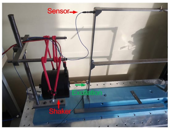
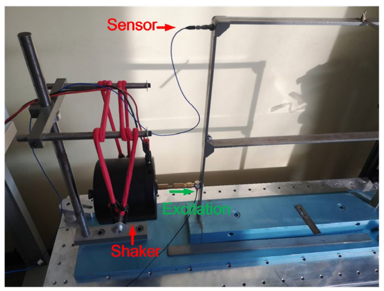
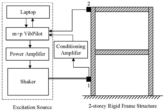
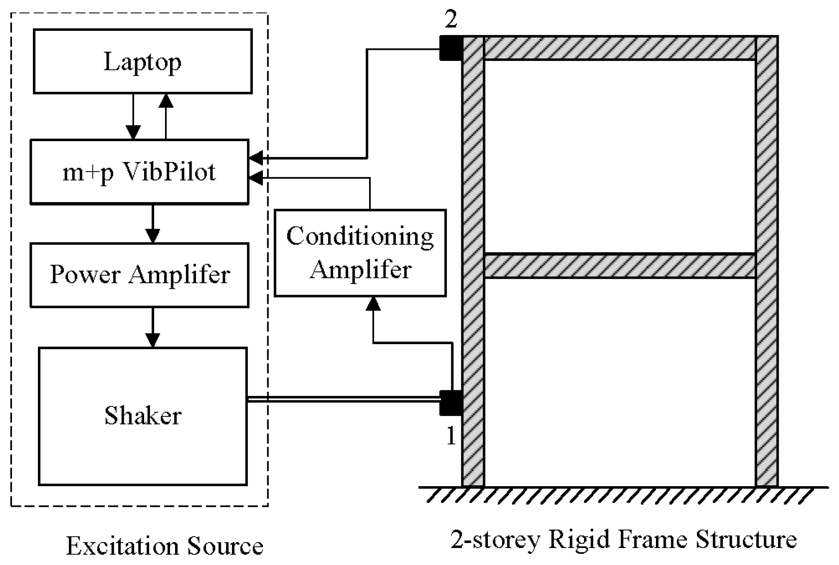
The experimental setup, shown in Figure 6. The structure is a two-story rigid frame made of steel, ensuring adequate stiffness and clear mass distribution. The structure was placed on a heavy steel table to provide a fixed boundary condition at its base. The excitation signal is designed in terms of noise distribution and amplitude using Matlab 2025b. It is then sent to the input/output acquisition board, amplified and converted into mechanical force by the shaker located near the clamped edge. The impedance head glued between the shaker head and the frame gives the input acceleration and force. Two accelerometers are located onto the frame. The signal from the accelerometers is sent back to the acquisition board, then visualized and saved.

Figure 6. Experimental set up.

A mechanical shaker, positioned on the left side of the structure, served as the dynamic excitation source. This shaker was connected to the structure through a force transducer, ensuring accurate measurement of the input force. By converting electrical signals into controlled mechanical vibrations, the shaker imposed horizontal dynamic loads that mimic a variety of excitation conditions, such as broadband noise or harmonic sweeps. The operating frequency range of the shaker and the input signal type (random, harmonic, or sweep) were adjustable, allowing for a thorough investigation of the structure’s frequency response and mode shapes.

Figure 7 shows a schematic diagram of the experimental setup. The setup consists of three main subsystems: (1) excitation source, (2) two-story rigid frame structure, and (3) data acquisition and processing. The experiment was conducted along the x-axis to ensure the structure behaved as a planar (2D) system. This simplification allowed for focused analysis on lateral dynamics, such as building sway, resonances, and energy dissipation mechanisms.

Figure 7. A schematic diagram of the experiment (1. force transducer, 2. accelerometer).

The excitation is provided by white noise, which stimulates all the eigenmodes of the structure within the frequency range up to half the sampling frequency (fs = 2048 Hz). The input signals consist of acceleration and force measurements obtained from an impedance head, while the output signal is the acceleration recorded by a piezoelectric accelerometer, model PCB M353B18. This accelerometer is attached to the beams using a magnet, and its placement is determined based on the specific mode being excited. Once again, the top floor mode will be studied.

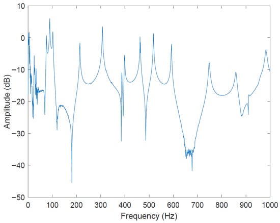
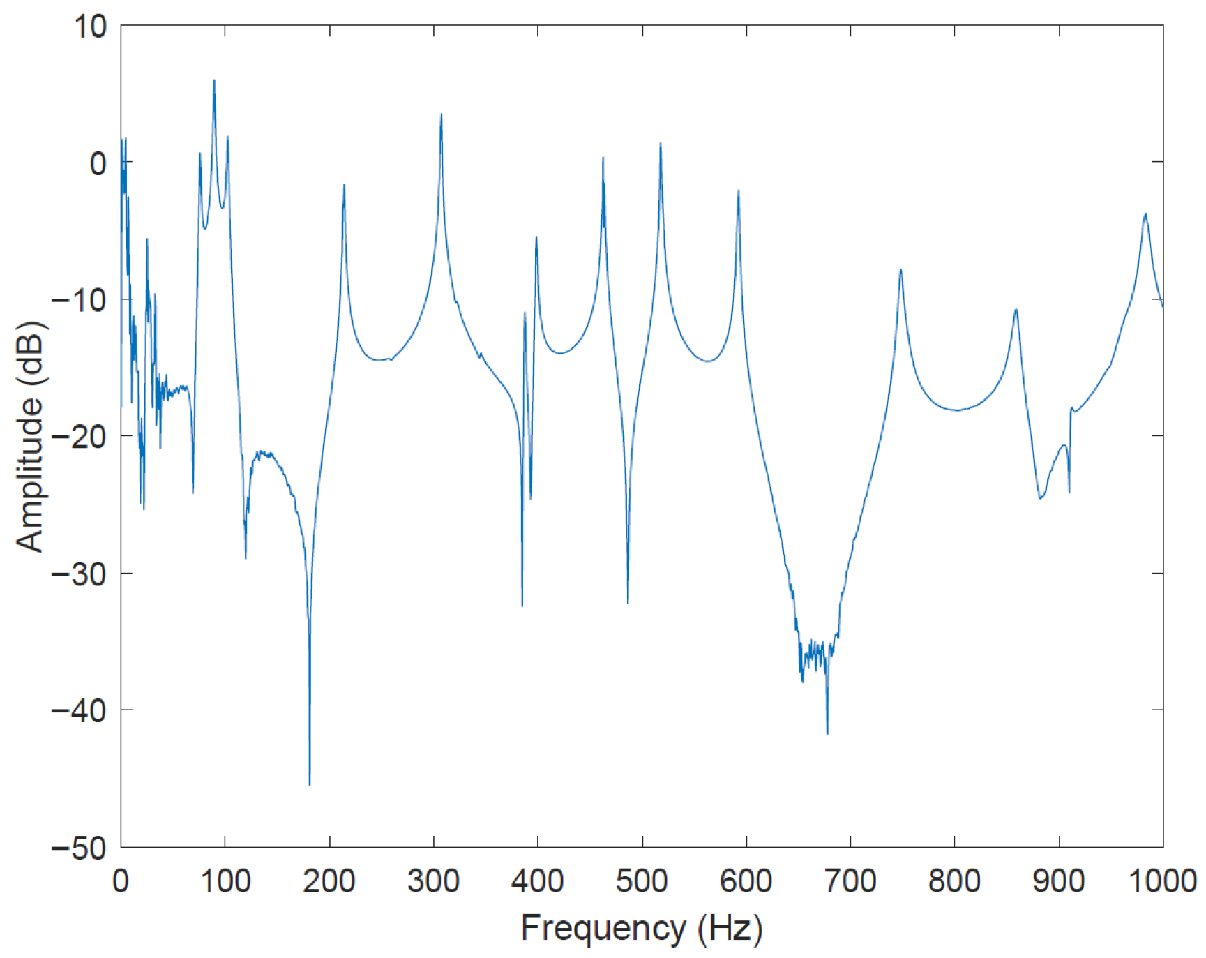
The FRF of the output acceleration divided by the input acceleration or the input force is represented in Figure 8. This figure has been obtained with ten measures of 1.6 s which smooths the results.

Figure 8. Experimental FRF of the mock building.

The FRF is noisy for frequencies up to 50 Hz due to the impedance head being unsuitable for low frequencies. However, the rest of the FRF shows the same tendencies as the previous one. In the two FRF, the resonance frequencies can be observed at the peak response, and are tabulated in Table 7.

Table 7. Eigenfrequencies of the first seven modes estimated from experimental FRFs and the full FEM model.

ith Mode	1	2	3	4	5	6	7
$f_i^{\exp }$ (Hz)	20.2	70.2	75.7	89.5	102.6	214	307
$f_i^{FEM}$ (Hz)	20.1	71	75.3	90	201	233	284

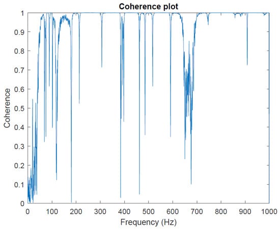
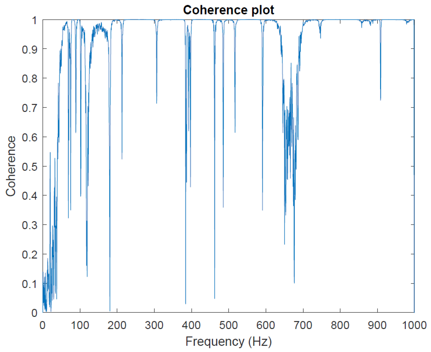
Moreover, a coherence plot has been realized to ensure that the results are valid for a frequency range used for the following work. It is a measure of a linear relationship between two signals. The coherence formula between two signals is given by:

$${\gamma }_{xy}^2(f)={\displaystyle \frac{|S_{xy}(f){|}^2}{S_{xx}(f)S_{yy}(f)}}$$

(71)

where:

• $S_{xx}$ represents the power spectral density of signal x.
• $S_{yy}$ represents the power spectral density of signal y.
• $S_{xy}$ is the cross power spectral density between two signals x and y.

The closer the coherence is to one, the better the relationship is between the different signals. Conversely, unrelated signals have a coherence close to zero. The following figure shows the coherence of the 10 blocks acquisition.

As shown in Figure 9, the coherence graphic demonstrates that once again, the data obtained from the instrumentation are valid for most frequencies above 50 Hz.

Figure 9. Coherence of the top point floor measurement point.

4.2. Impact of TMD on Vibration Response: Comparative Analysis

Despite significant advancements in vibration control and structural robustness, several challenges remain. These include accurately predicting the behavior of complex structures under stochastic excitation, taking into account uncertainties in TMD design, and effectively integrating machine learning models with traditional engineering approaches. Moreover, experimental validation of theoretical models in real-world scenarios remains a critical hurdle.

This section aims to demonstrate the integration of vibration control effectiveness using TMDs in a two-degree-of-freedom mass-spring system and extending this concept to a two-story building mock-up subjected to seismic-like excitation. This is achieved using experimental data from shaking tests to validate the performance of TMDs, then applying neural networks to define robustness domains based on experimental data and improve the predictive capabilities for structural reliability.

In addition to the FPT-based reliability assessment, the effectiveness of the TMD is also reflected in the modification of key dynamic characteristics, including shifts in natural frequency, increased effective damping, and reduction in dynamic amplification.

4.2.1. Design of the Tuned Mass Damper

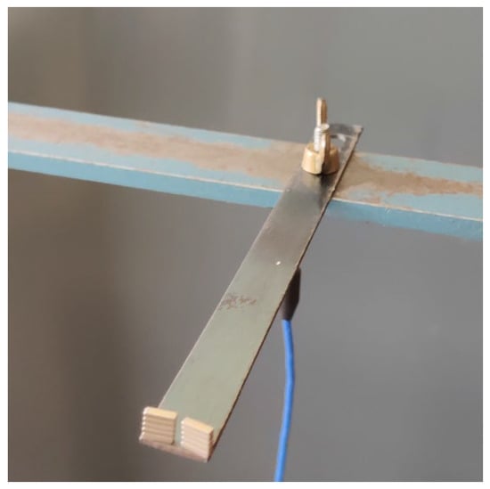
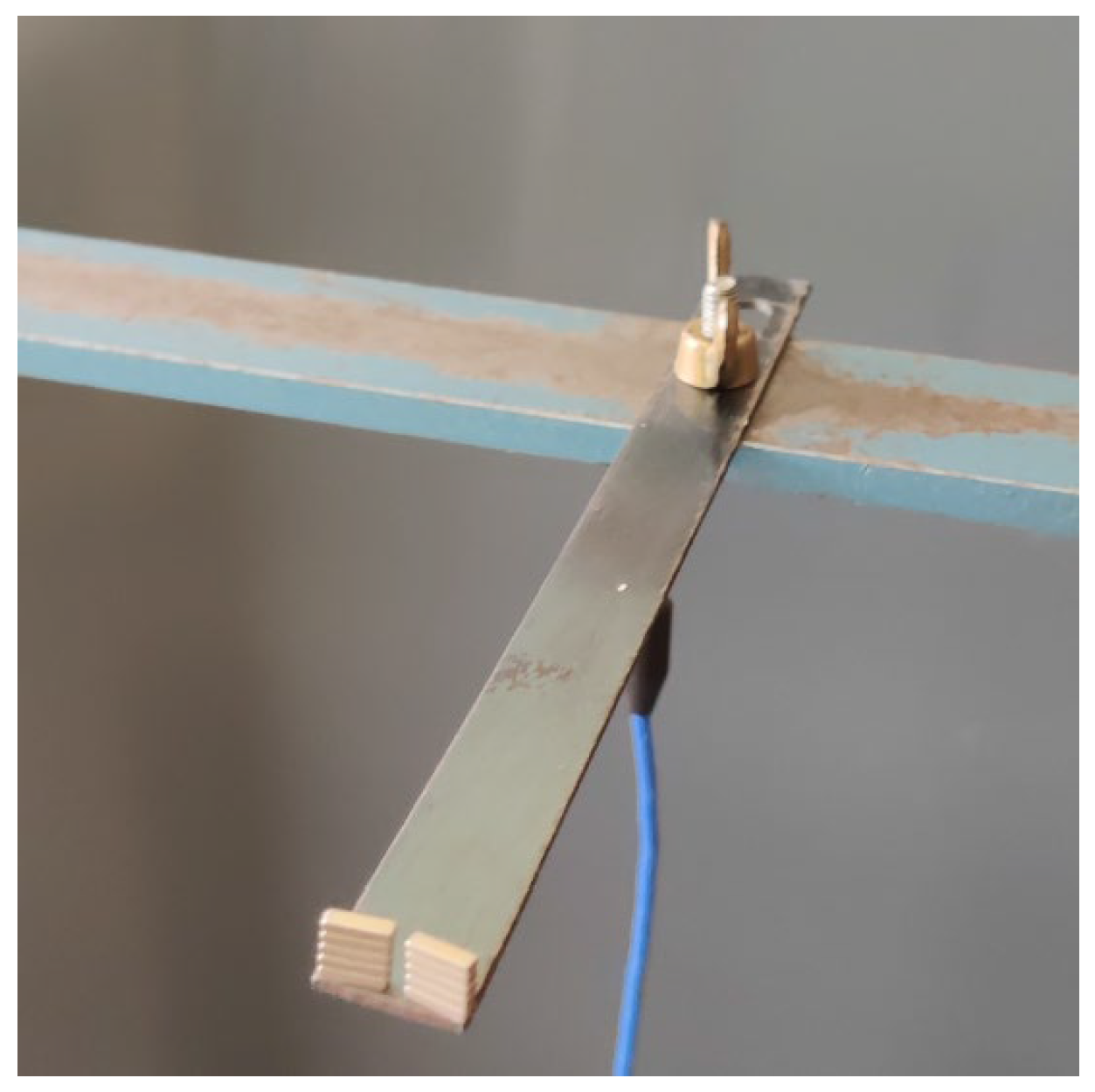
In this experiment, the TMD consists of a thin metal beam on which magnets are stuck, as shown in Figure 10.

Figure 10. The TMD in the experiment.

The following Table 8 outlines the key characteristics of the TMD:

Table 8. Characteristics of the TMD.

Characteristics	Value
Height	1 mm
Width	11 mm
Second moment of area	9.2 × 10−13 m4
Young modulus	210 GPa
Mass of one magnet	1 μg

The bar length can be adjusted between 94 mm and 110 mm, resulting in a corresponding variation in the TMD’s first resonance frequency according to the following formula:

$$f_{TMD}={\displaystyle \frac{1}{2\pi }}\sqrt{{\displaystyle \frac{11EI}{\left(\raisebox{1ex}{$4m_{TMD}$}\!\left/ \!\raisebox{-1ex}{$L$}\right.+\rho S\right)L^4}}}$$

(72)

To satisfy the Hartog criterion, the number of masses is chosen to achieve the desired first eigenfrequency of the damper.

4.2.2. Experimental Approach

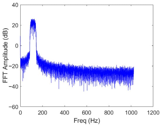
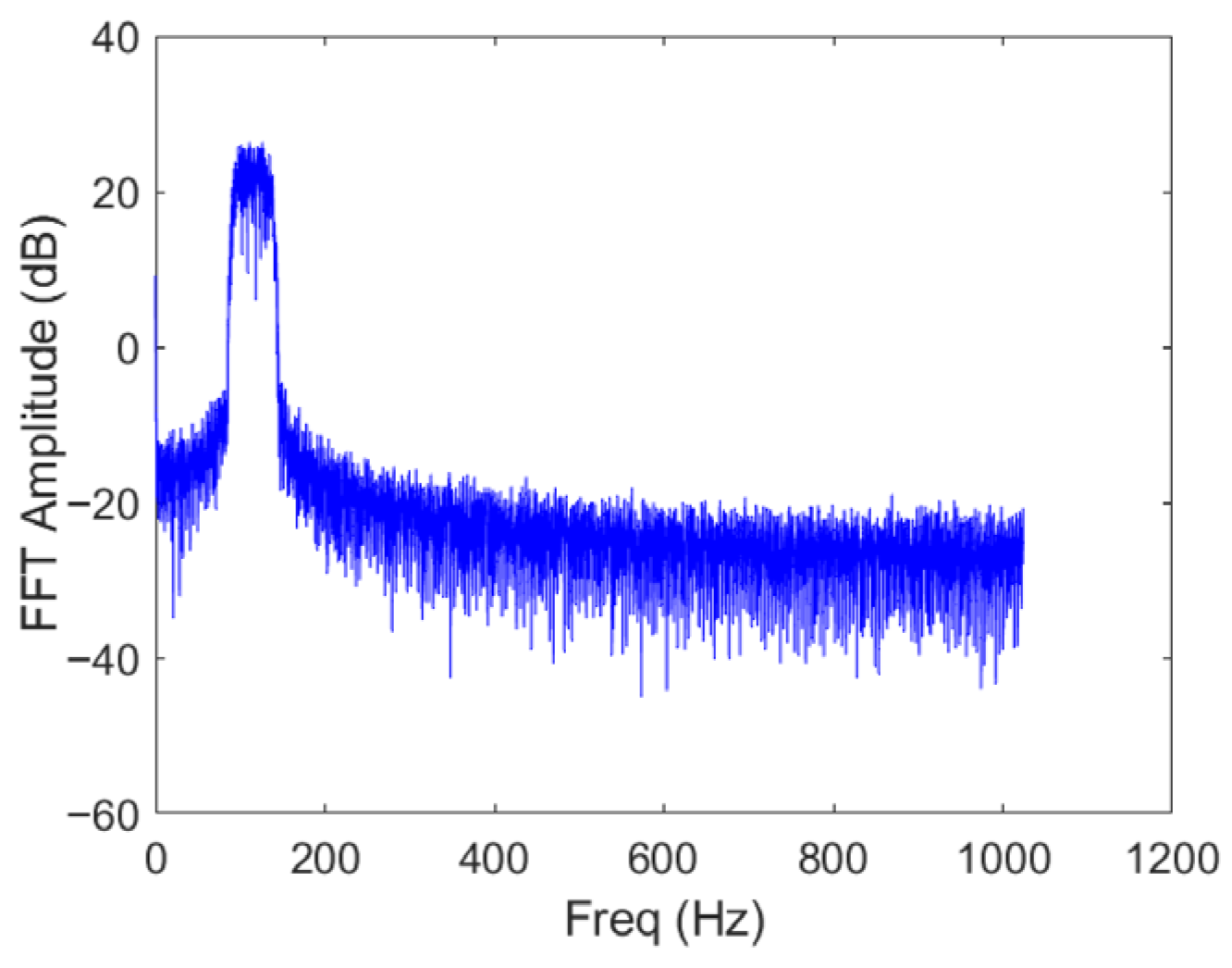
In this experiment, the response signals are measured by using an NI card connected to the MATLAB 2025b software. The advantage of MATLAB is that the inputs are easy to design. To represent a more realistic signal, the excitation is a Gaussian noise filtered between two frequencies: $f_{min}$ and $f_{max}$. The signal is windowed to avoid distortion. The acquisition lasts 10 s with a sampling frequency of 2048 Hz.

Figure 11 shows the FRF of the input signal. The FPT is extracted from the acceleration output. An acceleration threshold of arbitrary value is selected. If the threshold is not exceeded, the value assigned to the FPT is that of the maximum duration. Several measurements have been made with different input parameters. The goal is to predict the FPT knowing the input parameters. The parameters at stake are the maximal and minimal frequencies, and the amplitude of the noise. The FPT is extracted from the measured acceleration response by identifying the first instant at which the response exceeds a predefined threshold. This definition is consistent with the reliability framework adopted in the numerical analysis, enabling a direct comparison between experimental observations and simulation results.

Figure 11. FRF of the input signal.

4.2.3. First-Passage-Time Distribution from Experiments

In this section, distributions of the first-passage-time (FPT) distribution has been made in order to investigate the influence of the TMD on the first-passage time. Three different loading signals have been tested.

FPT Using Normal Distribution

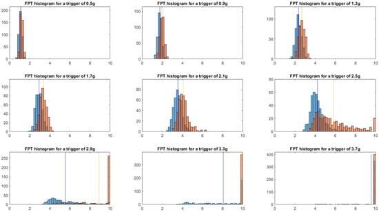
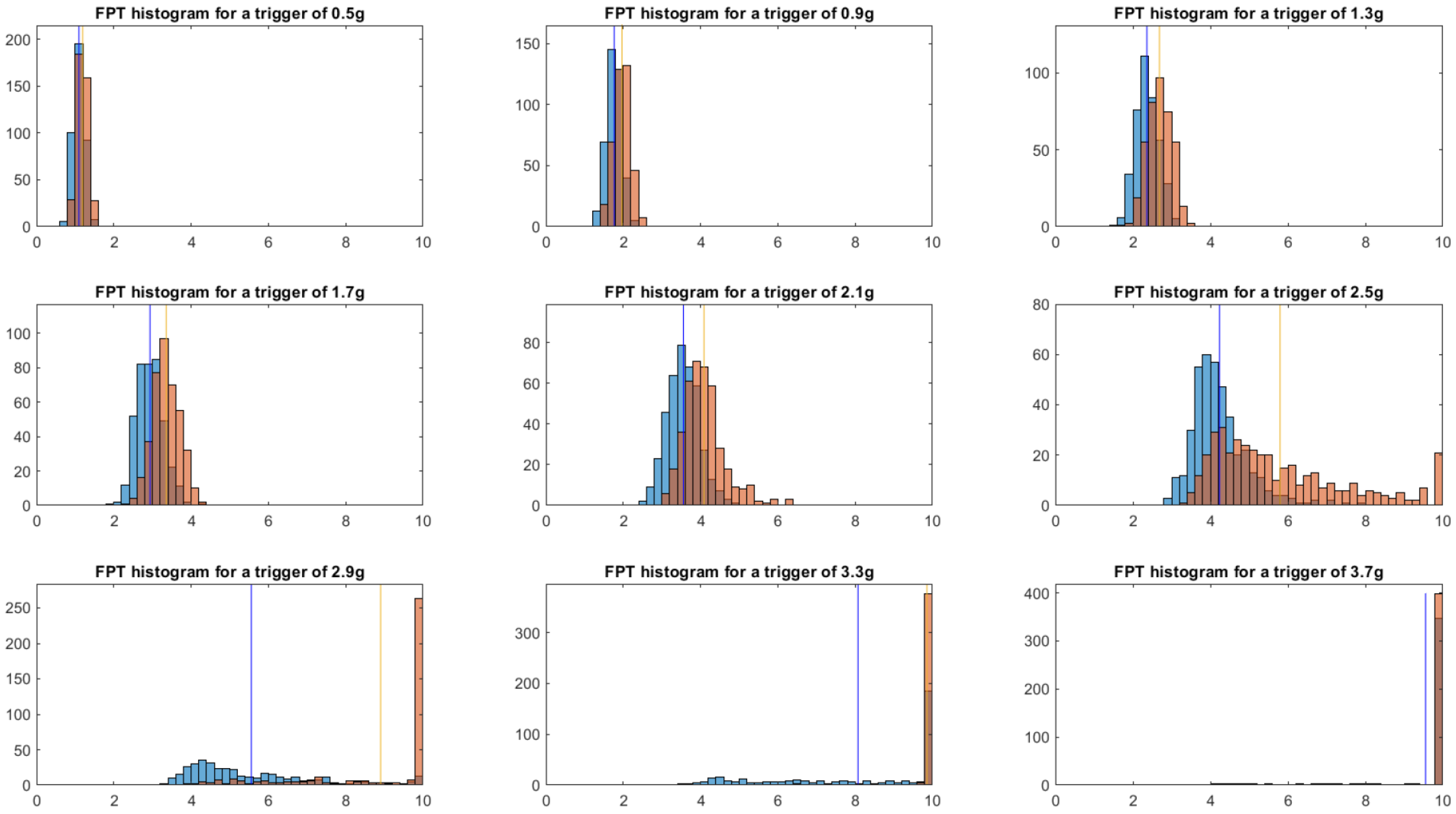
Measurements have been made with different excitation signals of ten seconds having the same properties, namely the maximal and minimal frequencies of the signal. Their values are respectively 60 Hz and 130 Hz. Figure 12 shows distributions of the FPT with or without a TMD, for various thresholds. When the thresholds have not been exceeded, the FPT is set to the test duration (10 s).

Figure 12. FPT histograms: orange with TMD, blue without. The vertical line shows the mean FPT. The x-axis is the FPT in seconds, y-axis is the occurrences.

As expected, the TMD increases the FPT of the structure, depending on the threshold level. Its effects are more noticeable for median thresholds. Moreover, the TMD tends to flatten the shape of the distribution.

FPT Using Other Distribution

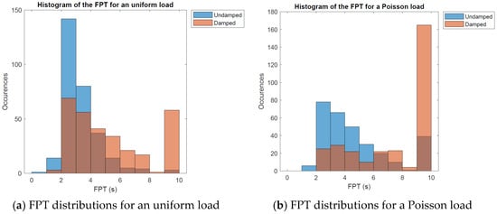
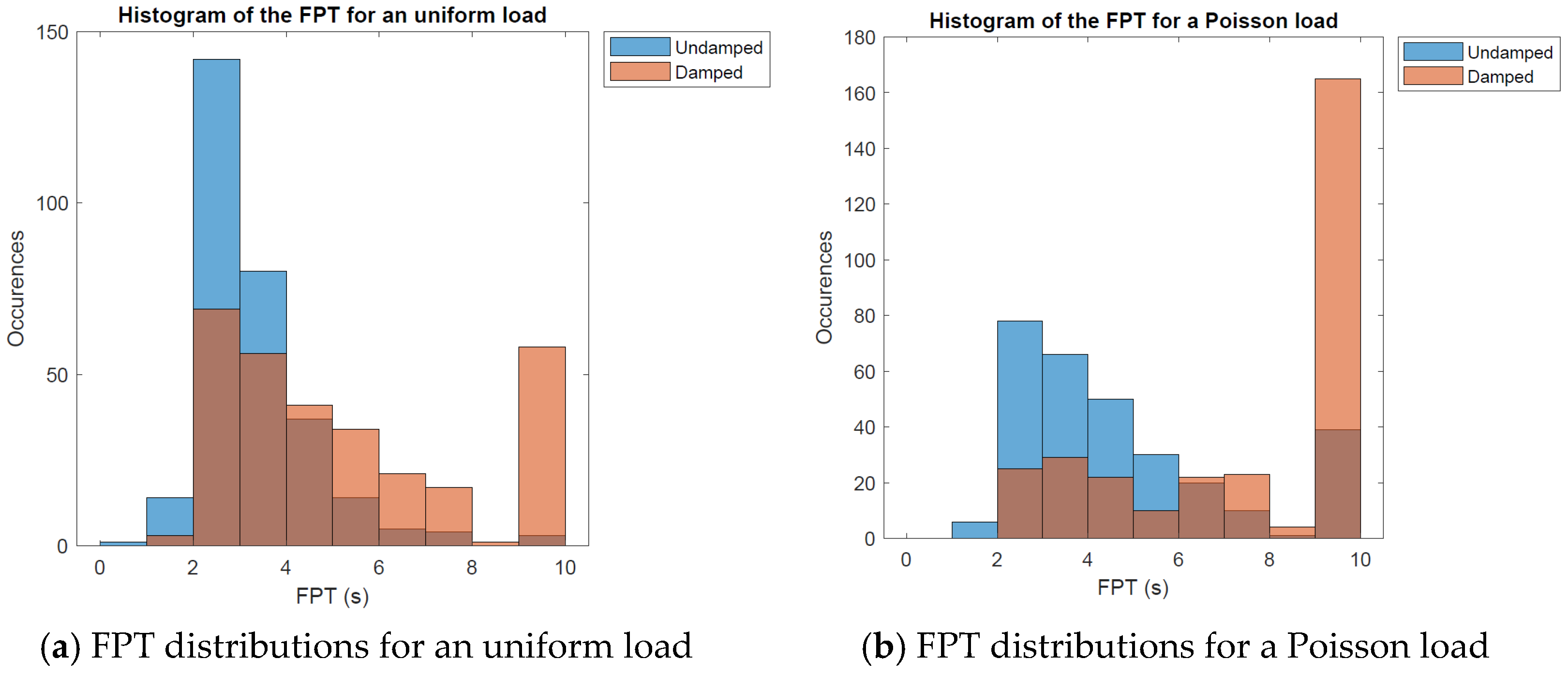
The properties of the entry signal can be changed in order to study the effects on the FPT. Two frequential distributions are considered. The uniform (Figure 13a) and the Poisson (Figure 13b) distribution, whose mean parameter λ is equal to 71 Hz (first floor mode).

Figure 13. FPT distributions.

As expected, the FPT is increased by the addition of the TMD, regardless of the distribution. Moreover, its seems the distribution of the load has an important effect on the FPT. The FPT distribution under uniform load is indeed more centered than the one under a Poisson law load. The uniform load excitates a large spectrum of frequencies, which may lead to degradation of the damping of the TMD, as it is tuned for only one frequency. That is why the Poisson load, which is frequencially centered around 71 Hz, may be more attenuated.

4.2.4. FPT Prediction Using Machine Learning

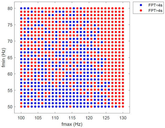
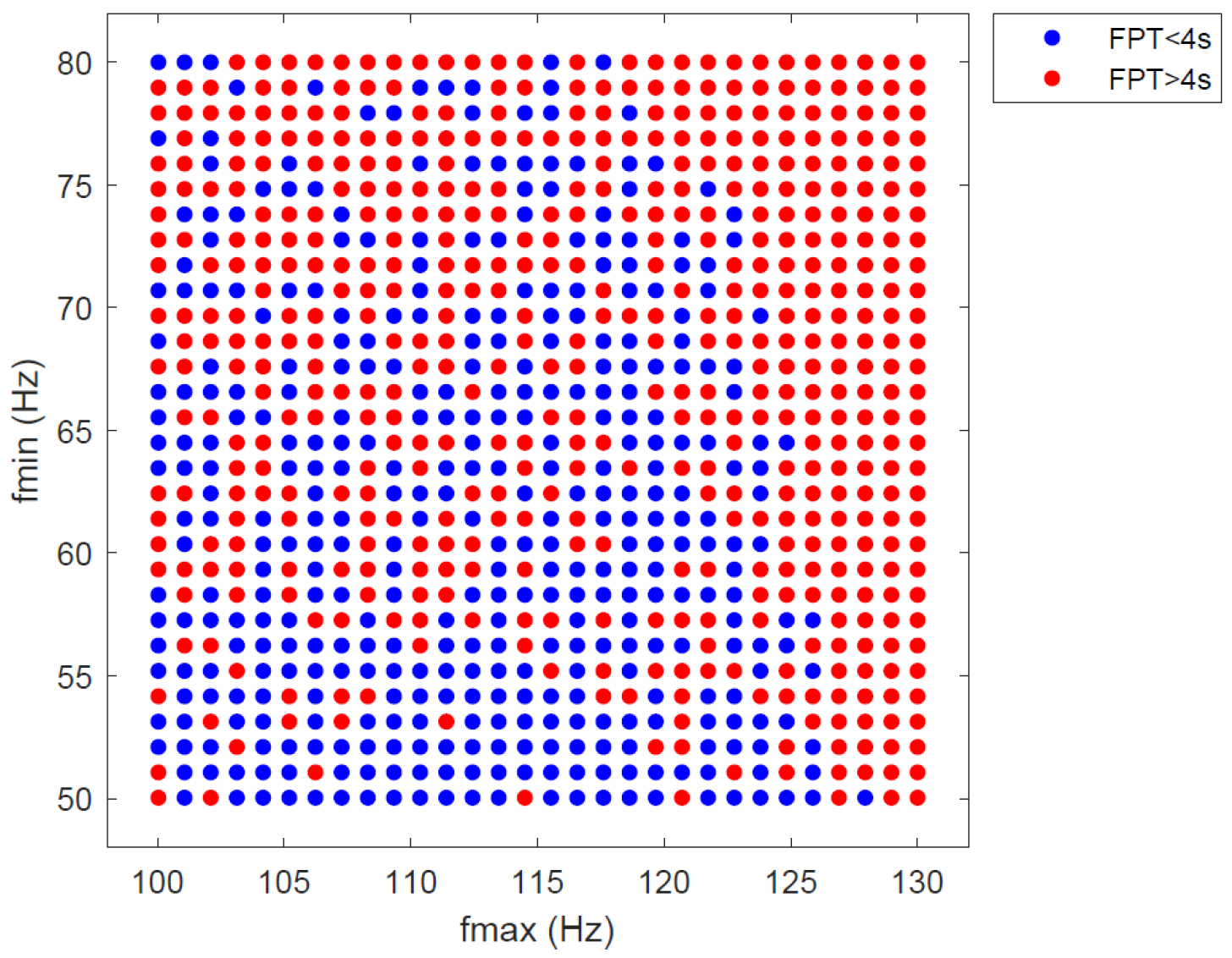
This part examines the impact of input features, such as filter frequencies, on the FPT. The setup described in the experiment is utilized to obtain the data. The features of interest are the maximal and minimal frequencies. To create a security domain for the structure, the values of FPT are considered, knowing that the threshold acceleration is 1.5 g. Two classes are created depending on if the FPT is inferior (failure domain) or superior to four seconds (security domain).

The minimum and maximum frequencies range from 50 to 80 Hz and from 100 to 130 Hz, respectively. Two datasets were created: (1) the training data, consisting of 900 measurements, and (2) the test data, consisting of 225 measurements conducted independently of the training data. The test data is crucial to evaluate the performances of the different algorithms. The security domain is represented by points worth one, conversely zero.

As shown in Figure 14, it sheds light upon the randomness characteristic of the FPT. Indeed, there is no clear separation between the two classes. It is possible to realize more classes, but this results in a poor separation of classes.

Figure 14. True FPT labels of the train data.

The two classes classification is used by classification programs, in order to predict the value of the FPT (inferior or superior to 4). Matlab offers a practical application that enables one to try multiple classification algorithms and compare their accuracy. As shown in Table 9:

Table 9. Validation and test accuracy of different classifiers.

Method	Validation Accuracy (%)	Test Accuracy (%)
Naive Bayes	71.3	75.6
Coarse KNN	71	73.8
SVM	71	75.1

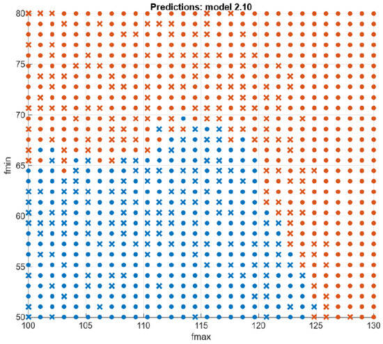
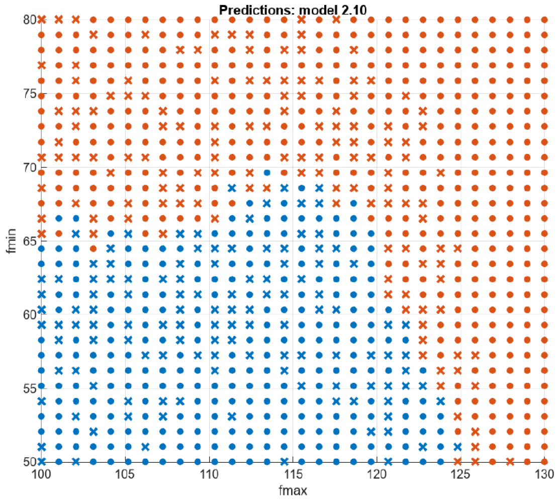
It can be seen from Figure 15 that the best classifier seems to be the Naive Bayes. Indeed, this method combines the best validation and test accuracies. These results show the efficiency of the KNN, Naive Bayes and SVM methods when it comes to classify a dataset with a low number of features.

Figure 15. Scatter plot of the training measures with the Naive Bayes method.

These results show that the usual machine learning methods are efficient to classify the FPT.

4.2.5. Impact of the Mass

In this part, the minimum frequency of the distribution is not considered. Instead, the focus is on studying the influence of the added mass from the TMD. The aim is to assess the impact of the TMD on the structure’s risk of failure and to train the neural network using this new set of data. Two series of measurements have been independently made in order to obtain train and test data. The test data consists of random values of added mass and maximal frequencies, and the associated FPT.

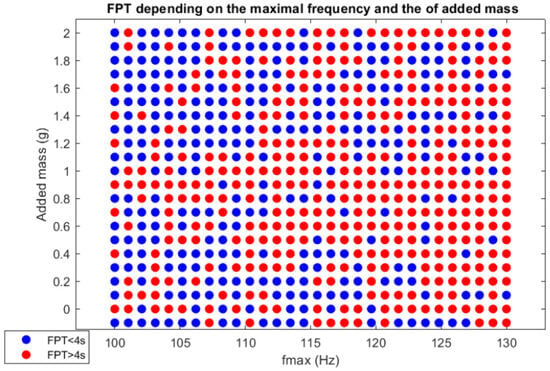
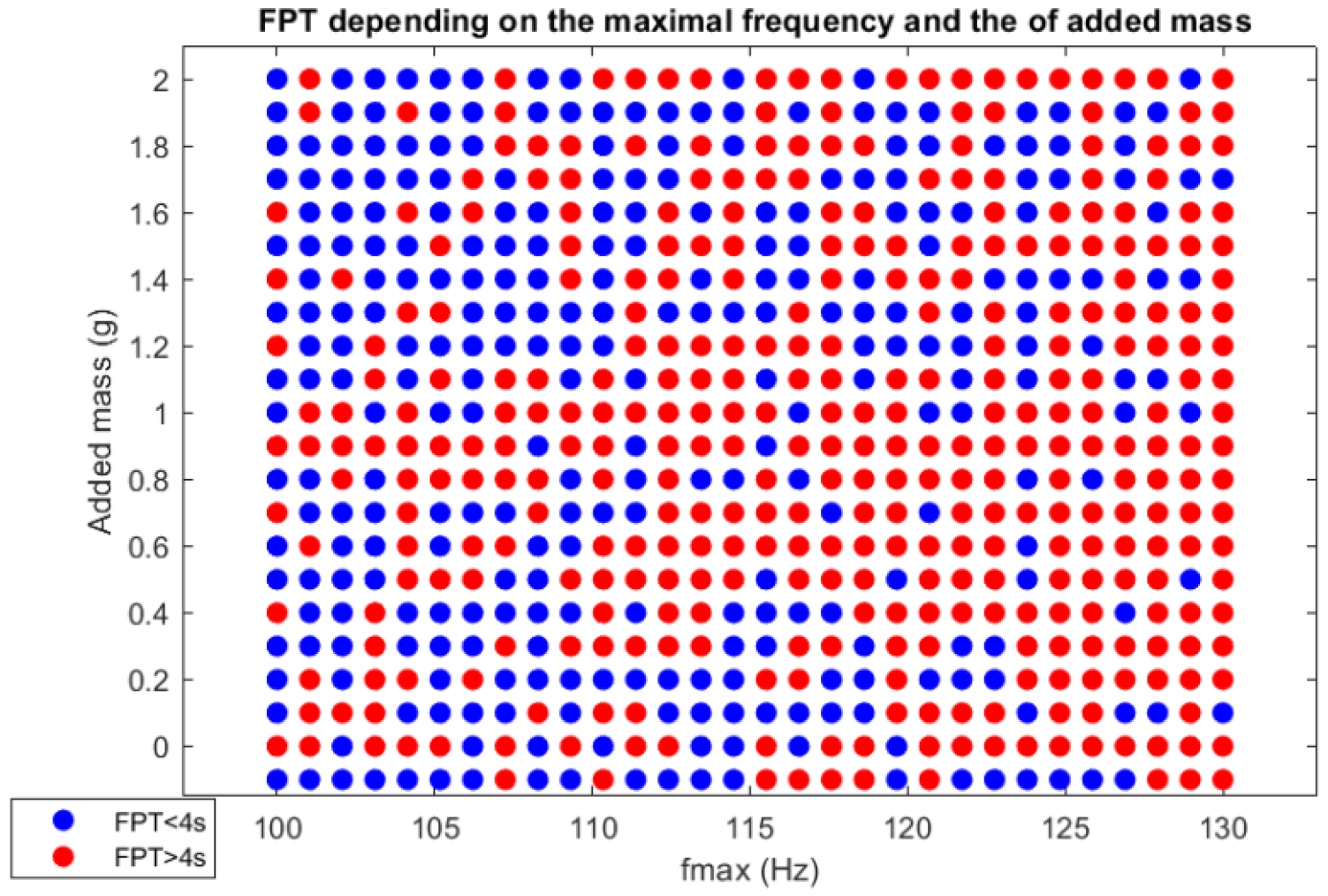
Figure 16 shows the influence of the added mass. The FPT is indeed almost always superior to four seconds when the added mass is close to 10 g. This mass tunes the first eigen frequency of the TMD close to one of the structures (71 Hz). In results, the TMD sufficiently damps the system and increases the FPT.

Figure 16. True FPT labels of the train data (add mass).

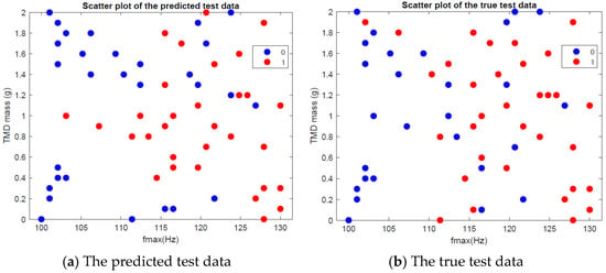
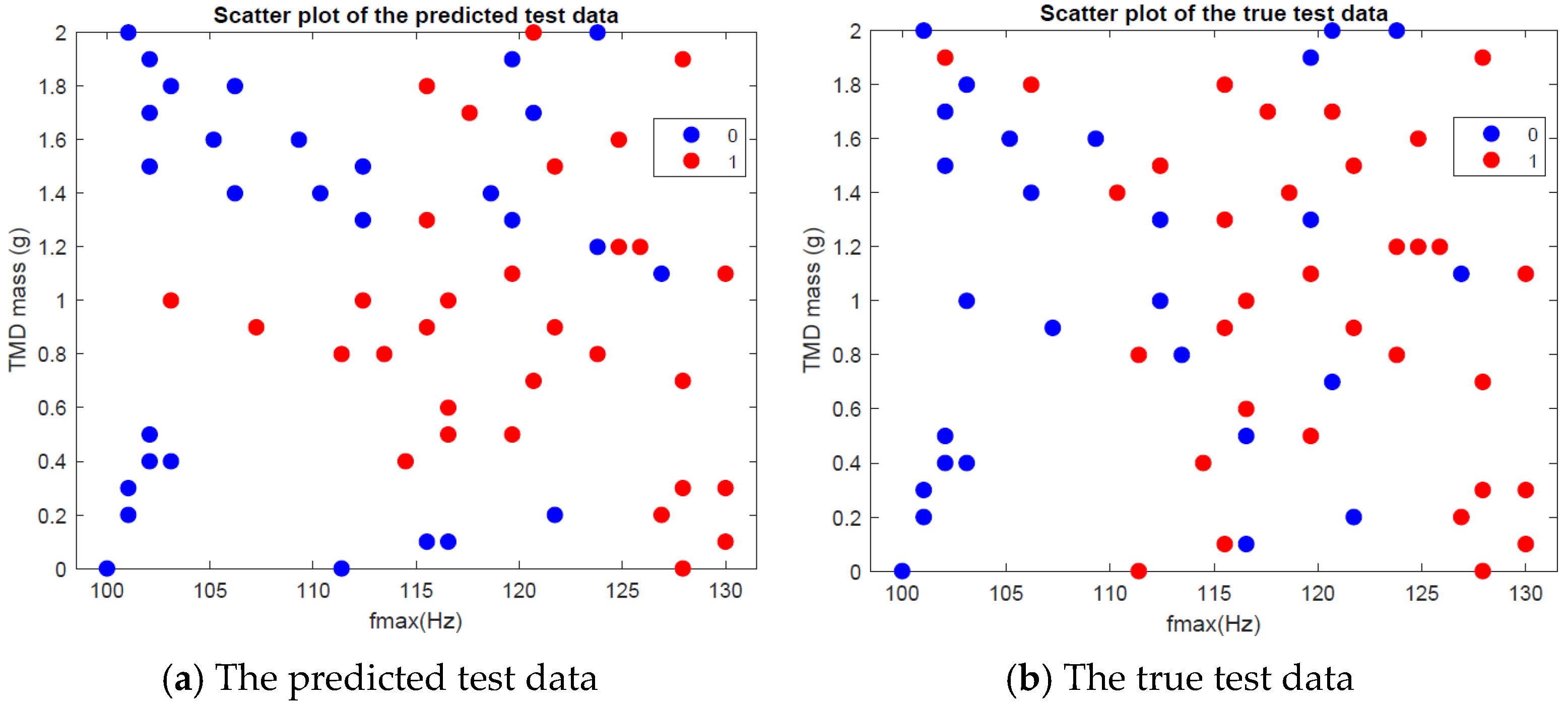
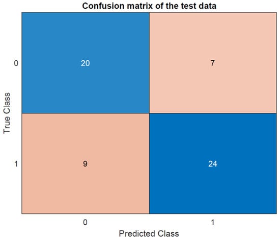
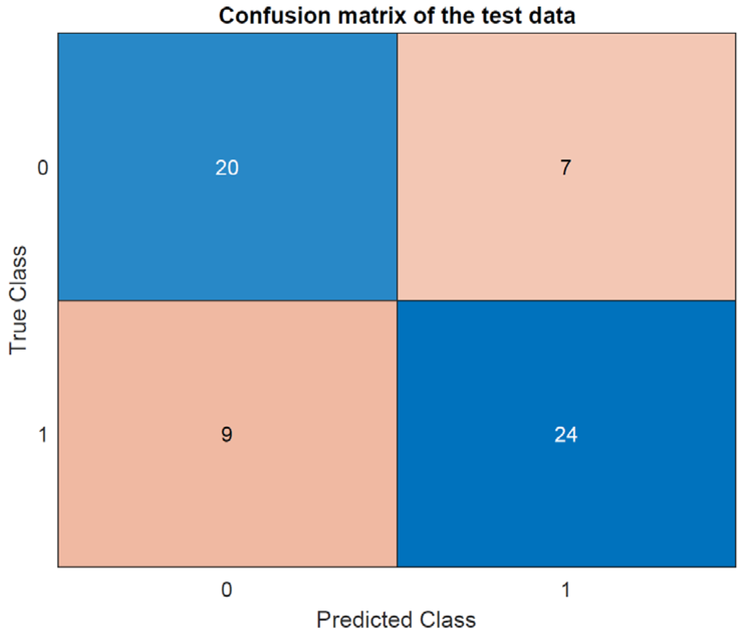
Next, an artificial neuron network is trained to learn the distribution. First, it uses the L-BFGS solver. The accuracy is 73.3% (Figure 17), and the confusion matrix is given in Figure 18.

Figure 17. Scatter plots of L-BFGS solver.

Figure 18. Confusion matrix of the L-BFGS solver predictions.

Use of another solver

The L-BFGS solver has a limited number of hyperparameters. It is possible to use other solver in order to compare the effectiveness of the classification. The RMSpropagation solver seems at first glance a good choice, as it is able to deal with noise in the dataset. RMSProp, which stands for root mean square propagation, is an adaptive learning rate optimization algorithm designed to address some of the issues encountered with the stochastic gradient descent.

The hyperparamters are the following:

• L2 regularization: this parameter reduces the effect of the variance of the data and reduces the weight of the loss function. This parameter helps in preventing overfitting.
• Initial learn rate: this parameter can prevent the gradient descent to converge to a local maximum that is not global, but when slows the convergence when too small.
• Max epoch: it is the number of times the whole training dataset is used during the learning phase.
• Mini batchsize: the number of training examples used to compute the gradient and update the model parameters in one forward and backward pass.

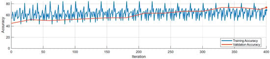
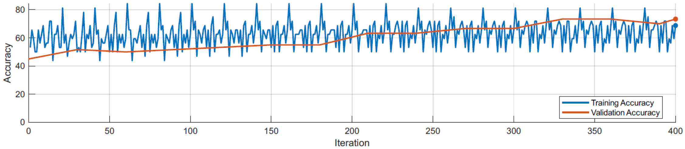
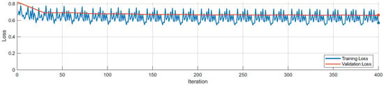
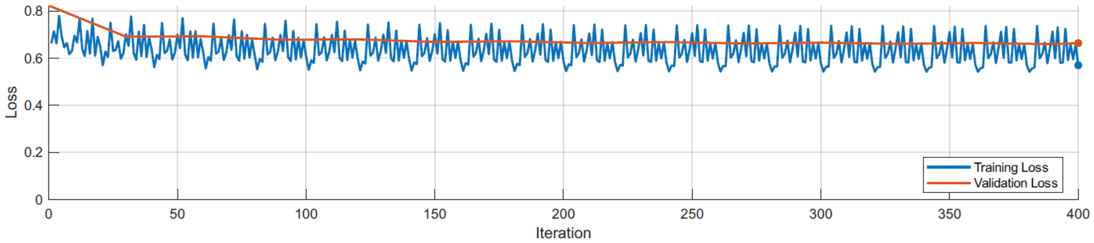
The accuracy and the loss evolution during the learning phase are shown in Figure 19 and Figure 20. The orange curb corresponds to the validation data that is used to monitor periodically the performances of the network. Once again, due to the noise of the data, the accuracy of the model does not converge to 100%.

Figure 19. Accuracy evolution during training.

Figure 20. Loss evolution during training.

4.2.6. Results Analysis

The results indicate that the first-passage time (FPT) can be accurately predicted using only the features of the input signals or the specific characteristics of the tuned mass damper (TMD). This finding is significant as it suggests that complex models or additional external data may not be necessary to achieve reliable predictions of FPT.

By leveraging key features such as the frequency content, amplitude, and phase of the input signals, as well as the design parameters of the TMD—such as its mass, damping coefficient, and natural frequency—the model can effectively anticipate when the system is likely to reach a critical threshold. The accuracy of these predictions is noteworthy, demonstrating that the selected features are sufficient to capture the essential dynamics of the system.

The L-BFGS solver, which is a quasi-Newton method, is relatively straightforward to implement due to its limited number of hyperparameters, making it a more user-friendly option for practical applications. On the other hand, the RMSProp solver, an adaptive learning rate method, involves a greater number of hyperparameters. While this complexity allows for finer tuning and potentially more robust performance in certain scenarios, it also requires more careful calibration and expertise during implementation. These differences highlight the trade-offs between simplicity and flexibility when choosing the appropriate solver for neural network training in this context.

4.2.7. Computational Efficiency Analysis

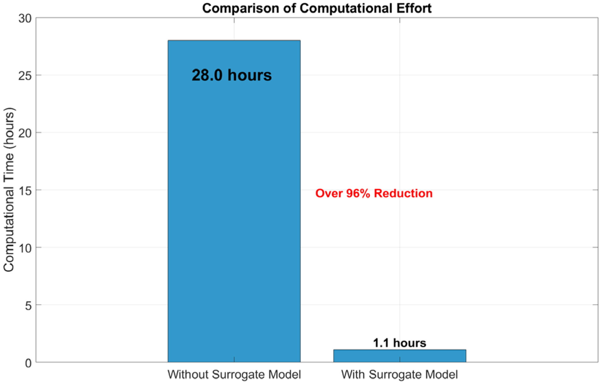
To further evaluate the computational efficiency of the proposed approach, the computational cost associated with the reliability analysis of the 10-DOF system is examined. Without the surrogate model, each stochastic dynamic simulation requires approximately 10 s on average, and a direct Monte Carlo simulation with 10,000 realizations would therefore take about 28 h of computational time.

By contrast, the training of the surrogate model requires approximately 1 h. Once the model is trained, the prediction of structural displacement for each realization takes about 0.01 s. As a result, the total computational time for 10,000 simulations is reduced to approximately 1.1 h, including the training process.

Overall, the proposed surrogate-assisted framework achieves a reduction of more than 90% (shown in Figure 21) in computational effort compared with the direct simulation-based approach. This significant improvement in efficiency demonstrates the suitability of the proposed method for reliability analysis of complex structural systems under stochastic excitation.

Figure 21. Computational cost comparison.

5. Conclusions

This work provides an integrated framework combining stochastic dynamics, reliability analysis, machine learning, and experimental validation for TMD-equipped structures.

To address the high computational cost of conventional Monte Carlo simulation, a data-driven surrogate model was introduced to approximate the system response. The surrogate model significantly reduced the computational effort while maintaining satisfactory accuracy in reliability estimation. Numerical studies on multi-degree-of-freedom systems demonstrated that the proposed approach can achieve reliable results with a substantial reduction in simulation time, making it suitable for large-scale reliability analysis.

In addition, the influence of stochastic excitation and parameter uncertainties on the reliability performance of TMD-controlled structures was systematically investigated. The results show that uncertainties play a non-negligible role in first-passage reliability and should be considered in practical vibration control design. Experimental validation further confirmed the effectiveness of the proposed framework and its potential applicability to real engineering systems. The results indicate that the variation in key parameters significantly affects the failure probability. In particular, parameters such as density and stiffness influence both the dynamic response amplitude and the likelihood of threshold exceedance. The presence of the TMD modifies the system dynamics by reducing vibration amplitude and increasing effective damping, which contributes to improved reliability performance.

Overall, the proposed methodology provides an efficient and practical tool for reliability assessment of TMD-equipped structures under stochastic loading conditions. This study is primarily applicable to linear structural systems under stationary stochastic excitation, while its extension to nonlinear behavior, non-Gaussian excitations, and large-scale complex structures remains a limitation that requires further investigation. Future work will focus on extending the framework to nonlinear systems and more complex excitation scenarios, as well as its application to full-scale engineering structures and real-time monitoring contexts.

References

- Yang, F.; Sedaghati, R.; Esmailzadeh, E. Vibration suppression of structures using tuned mass damper technology: A state-of-the-art review. J. Vib. Control 2022, 28, 812–836. [Google Scholar] [CrossRef] [Scilit]
- Rahimi, F.; Aghayari, R.; Samali, B. Application of tuned mass dampers for structural vibration control: A state-of-the-art review. Civ. Eng. J. 2020, 6, 1622–1651. [Google Scholar] [CrossRef] [Scilit]
- Rathi, A.K.; Chakraborty, A. Reliability-based performance optimization of tmd for vibration control of structures with uncertainty in parameters and excitation. Struct. Control Health Monit. 2017, 24, e1857. [Google Scholar] [CrossRef] [Scilit]
- Ghosh, A.; Basu, B. A closed-form optimal tuning criterion for tmd in damped structures. Struct. Control Health Monit. Off. J. Int. Assoc. Struct. Control Monit. Eur. Assoc. Control Struct. 2007, 14, 681–692. [Google Scholar] [CrossRef] [Scilit]
- Marian, L.; Giaralis, A. Optimal design of inerter devices combined with tmds for vibration control of buildings exposed to stochastic seismic excitation. In Safety, Reliability, Risk and Life-Cycle Performance of Structures and Infrastructures-Proceedings of the 11th International Conference on Structural Safety and Reliability, ICOSSAR 2013; CRC Press: Boca Raton, FL, USA, 2013; pp. 1025–1032. [Google Scholar]
- Zhang, D.K.; Kidd, D.W.; Varga, K. Excited biexcitons in transition metal dichalcogenides. Nano Lett. 2015, 15, 7002–7005. [Google Scholar] [CrossRef] [Scilit] [PubMed]
- Roy, A.; Chakraborty, S. Support vector machine in structural reliability analysis: A review. Reliab. Eng. Syst. Saf. 2023, 233, 109126. [Google Scholar] [CrossRef] [Scilit]
- Chun, J.; Song, J.; Paulino, G.H. System-reliability-based design and topology optimization of structures under constraints on first-passage probability. Struct. Saf. 2019, 76, 81–94. [Google Scholar] [CrossRef] [Scilit]
- Sun, J.Q.; Hsu, C. First-passage time probability of non-linear stochastic systems by generalized cell mapping method. J. Sound Vib. 1988, 124, 233–248. [Google Scholar] [CrossRef] [Scilit]
- Kulkarni, V.G. Modeling and Analysis of Stochastic Systems; Chapman and Hall/CRC: Boca Raton, FL, USA, 2016. [Google Scholar]
- Song, S.; Lu, Z.; Qiao, H. Subset simulation for structural reliability sensitivity analysis. Reliab. Eng. Syst. Saf. 2009, 94, 658–665. [Google Scholar] [CrossRef] [Scilit]
- Au, S.K.; Ching, J.; Beck, J.L. Application of subset simulation methods to reliability benchmark problems. Struct. Saf. 2007, 29, 183–193. [Google Scholar] [CrossRef] [Scilit]
- Rao, S.S. Vibration of Continuous Systems; John Wiley & Sons: Hoboken, NJ, USA, 2019. [Google Scholar]
- Burton, J.; Zinober, A.S. Continuous approximation of variable structure control. Int. J. Syst. Sci. 1986, 17, 875–885. [Google Scholar] [CrossRef] [Scilit]
- Igusa, T.; Der Kiureghian, A. Response of uncertain systems to stochastic excitation. J. Eng. Mech. 1988, 114, 812–832. [Google Scholar] [CrossRef] [Scilit]
- Dubourg, V.; Sudret, B.; Deheeger, F. Metamodel-based importance sampling for structural reliability analysis. Probabilistic Eng. Mech. 2013, 33, 47–57. [Google Scholar] [CrossRef] [Scilit]
- Shao, L. A Unified Surrogate Framework for Datadriven Reliability Insights in Mechanical Systems. Ph.D. Thesis, École Centrale de Lyon, Lyon, France, 2025. Available online: https://theses.hal.science/tel-05088884v1/document (accessed on 18 February 2025).
- Patel, J.; Choi, S.K. Classification approach for reliability-based topology optimization using probabilistic neural networks. Struct. Multidiscip. Optim. 2012, 45, 529–543. [Google Scholar] [CrossRef] [Scilit]
- Lieu, Q.X.; Nguyen, K.T.; Dang, K.D.; Lee, S.; Kang, J.; Lee, J. An adaptive surrogate model to structural reliability analysis using deep neural network. Expert Syst. Appl. 2022, 189, 116104. [Google Scholar] [CrossRef] [Scilit]
- Ontiveros-Pérez, S.P.; Miguel, L.F.F. Reliability-based optimum design of multiple tuned mass dampers for minimization of the probability of failure of buildings under earthquakes. Structures 2022, 42, 144–159. [Google Scholar] [CrossRef] [Scilit]
- Li, H.; Chen, H.; Zhang, J.; Chen, G.; Yang, D. Direct probability integral method for reliability sensitivity analysis and optimal design of structures. Struct. Multidiscip. Optim. 2023, 66, 200. [Google Scholar] [CrossRef] [Scilit]
- Shirgir, S.; Shamsaddinlou, A.; De Domenico, D. Reliability-Based Design Optimization of Tuned Mass Damper for Tall Buildings Considering Uncertainty of Soil-Structure Interaction. Struct. Des. Tall Spec. Build. 2025, 34, e70075. [Google Scholar] [CrossRef] [Scilit]
- Rizzo, F. Investigation of the time dependence of wind-induced aeroelastic response on a scale model of a high-rise building. Appl. Sci. 2021, 11, 3315. [Google Scholar] [CrossRef] [Scilit]
- Bhowmik, K.; Debnath, N. Stochastic design of multiple tuned mass damper system under seismic excitation. Arch. Appl. Mech. 2022, 92, 383–404. [Google Scholar] [CrossRef] [Scilit]
- Mrabet, E.; Soula, M.; Guedri, M.; Ghanmi, S.; Ichchou, M. Stochastic optimal design of tuned mass damper parameters using energetic approaches. In Design and Modeling of Mechanical Systems-II: Proceedings of the Sixth Conference on Design and Modeling of Mechanical Systems, CMSM’2015, March 23–25, Hammamet, Tunisia; Springer International Publishing: Cham, Switzerland, 2015. [Google Scholar]
- Peng, Y.; Sun, P. Reliability-based design optimization of tuned mass-damper-inerter for mitigating structural vibration. J. Sound Vib. 2024, 572, 118166. [Google Scholar] [CrossRef] [Scilit]
- Chen, K.; Hou, J.; Ding, L.; Wang, Q.; Huang, Y.; Xiao, Z.; Liu, Z.; Tang, X.; Wu, Y.; Zeng, Q.; et al. Hierarchical Amorphous–Crystalline Ceramic Nanotube Array Nanocomposites with Superior Mechanical and Functional Properties. Adv. Mater. 2026, 38, e13101. [Google Scholar] [CrossRef] [Scilit] [PubMed]
- Anand, R.; Tripathi, S.; De Oliveira, C.C.; Malla, R.B. Field-Test-Driven Sensitivity Analysis and Model Updating of Aging Railroad Bridge Structures Using Genetic Algorithm Optimization Approach. Infrastructures 2025, 10, 195. [Google Scholar] [CrossRef] [Scilit]
Disclaimer/Publisher’s Note: The statements, opinions and data contained in all publications are solely those of the individual author(s) and contributor(s) and not of MDPI and/or the editor(s). MDPI and/or the editor(s) disclaim responsibility for any injury to people or property resulting from any ideas, methods, instructions or products referred to in the content. |
© 2026 by the authors. Licensee MDPI, Basel, Switzerland. This article is an open access article distributed under the terms and conditions of the Creative Commons Attribution (CC BY) license.