3D Inversion of Underground Concealed Coal Fire Sources Based on Self-Potential Data in Xinjiang, China

Abstract

Accurate localization of concealed fire sources is the fundamental prerequisite for effective coal fire control and mitigation. The self-potential method, as a passive, cost-effective geophysical technique for large-area surveys, exhibits unique advantages in coal fire detection, yet 3D inversion of self-potential data for high-precision coal fire source localization remains insufficiently studied. In this paper, a 3D iterative compact inversion algorithm based on the minimum support functional is adopted to invert self-potential data for 3D localization of underground concealed coal fire sources. The algorithm’s reliability and robustness are verified systematically via numerical simulations at both laboratory and field scales, followed by sandbox experiments with artificial battery sources and burning coal specimens, and finally validated its engineering applicability in the Sandaoba Coal Fire Area in Xinjiang. Numerical results show that the algorithm achieves high-precision inversion of source current density across multiple orders of magnitude, with a relative error below 10%. Sandbox experiments confirm that coal combustion generates a typical dipole self-potential field with distinct negative surface anomalies, whose amplitude is positively correlated with combustion intensity. Field inversion results successfully delineate the 3D boundary of the concealed fire source (buried at 40–140 m), which is highly consistent with borehole temperature measurement data. This study provides a robust technical framework for 3D detection of concealed coal fires, offering strong technical support for precise coal fire governance and hazard mitigation.

1. Introduction

Coal fires are defined as uncontrollable combustion events occurring in underground coal seams, which are normally triggered by coal spontaneous combustion [1,2,3,4]. These fires can spread from localized areas to widespread uncontrolled burning, causing severe damage to coal resources and posing substantial environmental threats [5]. Besides wasting coal resources, coal fires also constitute a significant threat to ecological safety and social stability [6,7]. Xinjiang is the province in China most severely affected by coal fires. According to the fifth survey and supplementary investigation of coal fires in Xinjiang, there are 84 coal fires in the region, covering a total area of approximately 12.4 million square meters. These areas are mainly distributed in Changji Hui Autonomous Prefecture, Turpan City, Aksu City, Hami City, Ili Kazakh Autonomous Prefecture, and Urumqi City. These fires burn approximately 21.82 million tons of coal annually, emitting 54.71 million tons of carbon dioxide, 19,800 tons of nitrogen oxides, 80,700 tons of sulfur dioxide, and 192,300 tons of particulate matter each year. To mitigate its impact on the environment and human health, it is essential to implement effective control and management. A key prerequisite for achieving this goal is the precise identification of the underground coal fire source locations.

At present, the mainstream approaches for coal fire detection involve detecting underground physicochemical fields using various equipment. These techniques include remote sensing [8,9,10,11,12,13,14], borehole temperature and gas measurement [15,16,17], magnetic prospecting [18,19,20], radon detection [2,21,22,23,24], and electrical methods [2,25]—the latter covering transient electromagnetic, electrical resistivity tomography (ERT) [26], and self-potential method [16,27,28,29,30,31,32]. The merits and limitations of the above detection methods have been systematically analyzed in our prior publications [33,34] and thus will not be elaborated in detail here. Compared to other sophisticated geophysical exploration techniques, the self-potential method—a passive electrical geophysical prospecting approach—enables large-area coverage at relatively low costs, which supports the acquisition of more comprehensive geophysical datasets [34].

In general, temperature gradients in porous media drive charge carriers to migrate from warmer to cooler regions, which serves as the primary genesis of self-potential anomalies observed in coal fire areas. As an effective survey method, the self-potential method can detect electric field variations on the ground surface. By analyzing the distribution of the self-potential field, valuable information about the combustion state and location of the coal fire can be obtained. Many scholars have conducted related research on the application of the self-potential method. For example, Revil et al. [27] observed negative self-potential anomalies on the surface above heat sources in sandbox experiments, and recorded a peak negative anomaly of −50 mV in the Lewis fire area. Karaoulis et al. [16] deployed the self-potential method to investigate the Lewis fire area, detecting surface anomalies ranging from +70 mV to −50 mV and successfully pinpointing the combustion front of the fire source. Shao et al. [31] studied self-potential anomalies linked to coal fires, finding that anomaly amplitude increases with heat source temperature but drops sharply with greater burial depth. Srivardhan et al. [35] proposed a novel coal fire depth estimation method that integrates self-potential data with particle swarm optimization to achieve depth inversion. Furthermore, with the continuous refinement of self-potential inversion theory and the rapid advancement of computing technology, new interpretation frameworks for self-potential anomalies have emerged, and a wide range of nonlinear algorithms have been extensively applied in self-potential inversion research [30,36,37,38,39]. Owing to its operational convenience and real-time performance, the self-potential method is widely recognized as an effective tool for coal fire detection. Nevertheless, three-dimensional (3D) inversion of coal fire sources based on self-potential data remains largely underexplored in existing studies.

In this paper, five sandbox experiments with artificial battery sources and burning coal specimens are conducted to investigate the self-potential anomaly. The reliability and robustness of the inversion algorithm, which allows for iterative and compact inversion of the source’s current density, are verified systematically via numerical simulations at both laboratory and field scales before inverting sandbox experiment data. Self-potential data is collected at the Sandaoba Coal Fire Area in Xinjiang and the 3D location of the underground concealed fire source is obtained by the 3D inversion algorithm.

2. Sandbox Experiments

2.1. Material and Methods

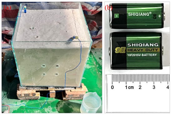
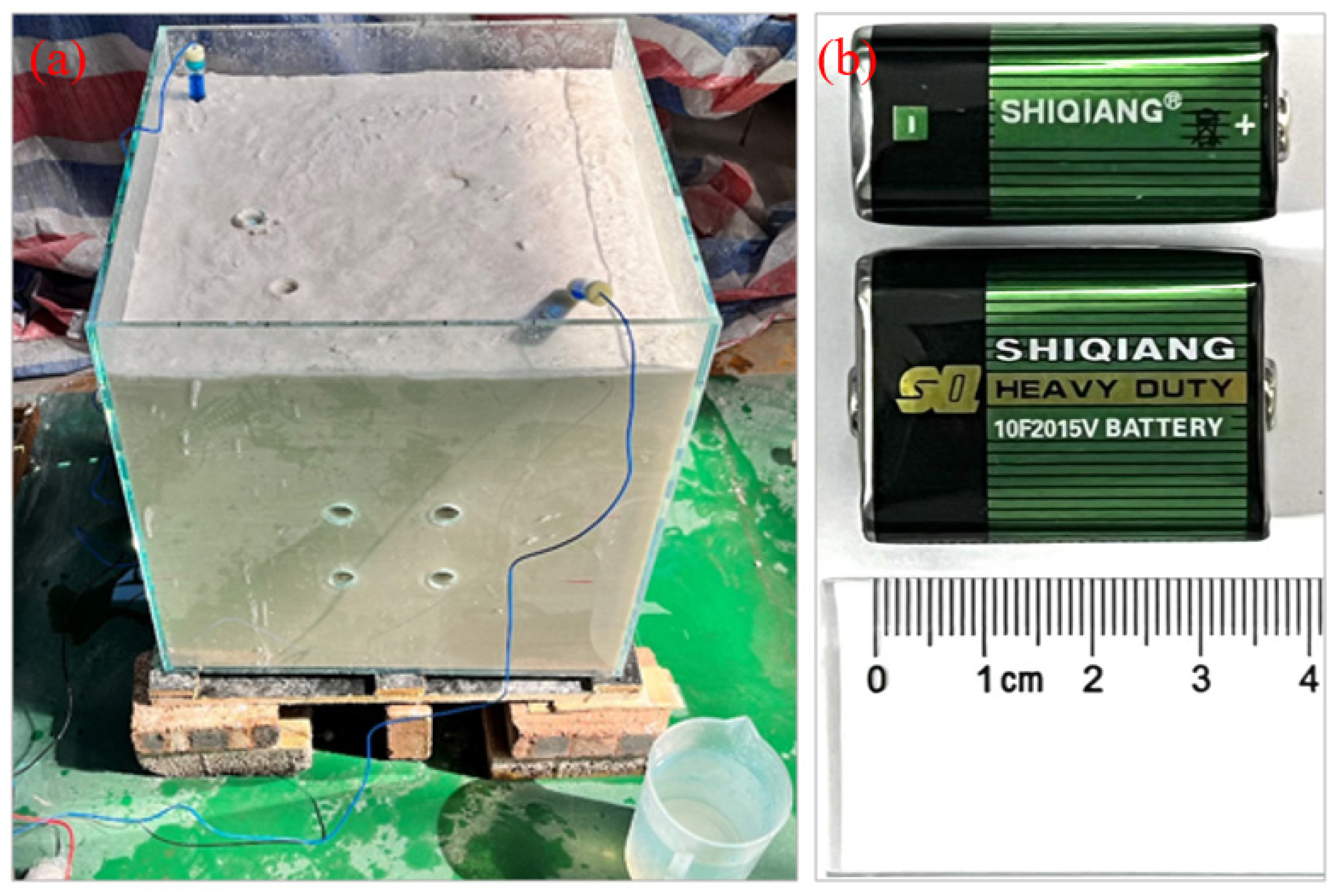
The sandbox used in the experiment is a transparent glass box with a thickness of 8 mm, and internal length, width, and height of 0.5 m. Quartz sand, with an average particle size of 120 ± 20 µm, is selected as the filling material to simulate the formation medium in the sandbox. In order to capture weak self-potential signals, the quartz sand is pre-saturated with water to ensure that the air in the quartz sand could be evacuated and to ensure the uniform conductivity throughout the sandbox. Then, the water-saturated quartz sand is filled to a height of 0.44 m, as illustrated in Figure 1a. The conductivity of tap water is 0.074 Sm⁻¹, and quartz sand has an electrical formation factor of approximately 3.6 at 25 °C [40]. Therefore, the conductivity of the saturated quartz sand can be calculated by the conductivity of water:

$${\sigma }_{sand}={\sigma }_{tw}{F}^{-1}$$

(1)

Figure 1. Photos of sandbox and battery used for the experiment. (a) Sandbox and nonpolarizing Cu-CuSO4 electrodes. (b) 15 V battery used in the experiment with the size of 3.6 cm × 2.5 cm × 1.6 cm.

In Equation (1), ${\sigma }_{sand}$ represents the electrical conductivity of water-saturated quartz sand, in Sm⁻¹; ${\sigma }_{tw}$ represents the electrical conductivity of tap water; and F represents the electrical formation factor. According to the formula, the electrical conductivity of water-saturated quartz sand is about 0.021 Sm⁻¹, which is equivalent to a resistivity of 47.62 Ωm.

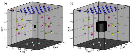
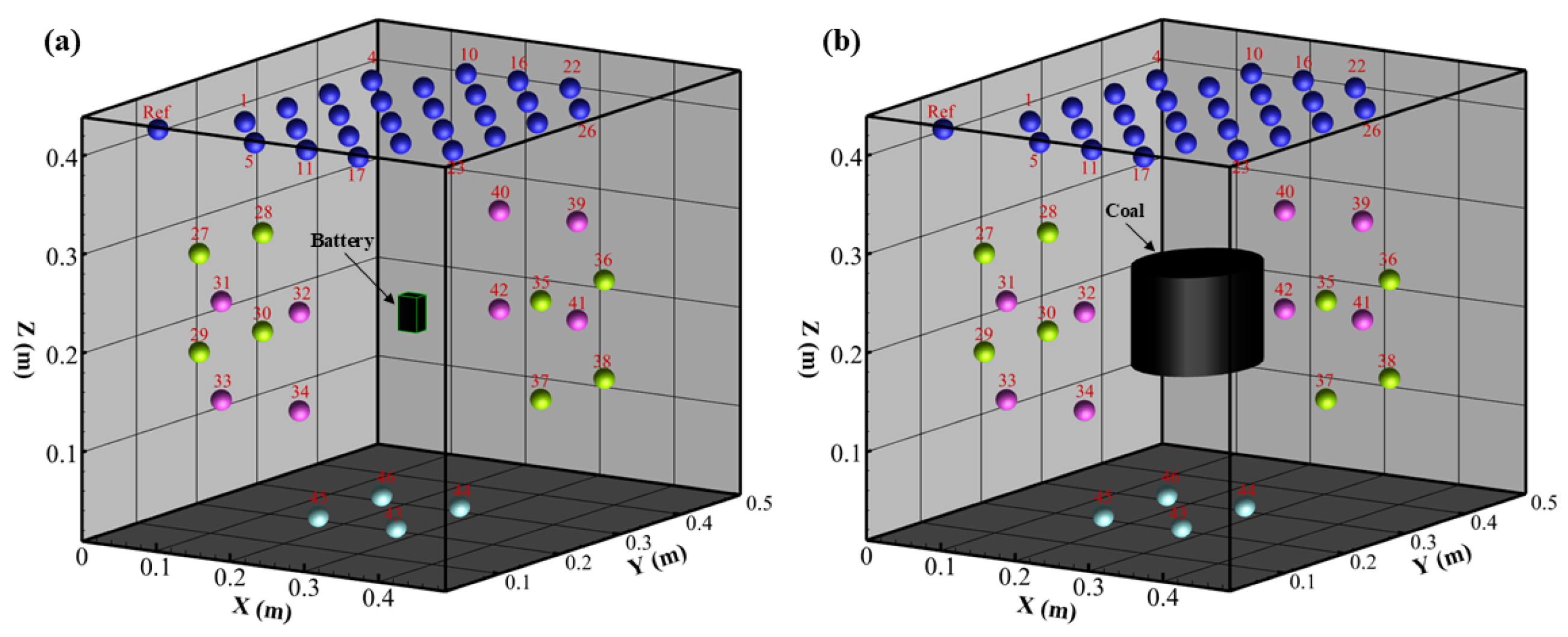
As illustrated in Figure 2a, a total of 46 measurement points is developed to collect self-potential data. Specifically, 26 measurement points are arranged on the upper surface of the sandbox, with an equal spacing of 7 cm between adjacent points. Four additional measurement points are set at the geometric center of the bottom side of the sandbox, with a spacing of 10 cm between adjacent boundary measurement points. The remaining 16 measurement points are distributed along the four lateral sides, with their elevations fixed at either 17 cm or 27 cm from the sandbox bottom. This measurement layout enabled the acquisition of self-potential data in the vertical direction, while also capturing the distribution characteristics of the self-potential field near the sandbox boundaries. To minimize the interference of reference electrode potential drift on individual self-potential measurements, the reference electrode is fixed at the corner of the sandbox upper surface (marked as Ref in Figure 2), consistent with the fixed reference point measurement method described previously.

Figure 2. Sketch of the sandbox used for the experiment with battery (a) and burning coal (b). The colored balls represent the measurement points. (Blue and light blue balls denote the top and bottom measurement points, respectively, while green and pink balls denote the side measurement points).

Prior to conducting the burning coal experiment, it is essential to characterize the self-potential response of a known artificial current source, to verify the reliability of the measurement system and validate the performance of the adopted inversion algorithm. The source of self-potential anomaly in coal fire areas is the distribution of the electric field in three-dimensional space caused by the dipole current source generated by the thermal–electric effect. The battery is a compact current source and is dipole in nature. It can provide a relatively stable current output as well as a continuous and controllable electric field, which is crucial for understanding the electrical field within the sandbox and verifying the experimental model. Therefore, in our sandbox experiments, the battery as a known artificial current source is used to simulate the burning coal fire source. Four battery simulation experiments (Experiments #1–#4) are designed under controlled variable conditions, with detailed experimental settings as follows:

(1)

Experiment #1: A single 15 V battery embedded at a depth of 11 cm.

(2)

Experiment #2: A single 15 V battery embedded at a depth of 22 cm.

(3)

Experiment #3: A single 15 V battery embedded at a depth of 33 cm.

(4)

Experiment #4: Two horizontally aligned 15 V batteries embedded side-by-side at a depth of 22 cm.

All batteries in the four experiments are horizontally centered in the sandbox, with their positive electrodes facing upward. By varying the embedded depth and number of battery sources, we systematically characterize the self-potential distribution on the upper surface of the sandbox, and establish the quantitative relationship between source parameters and surface self-potential anomaly characteristics.

Experiment #5 is designed to investigate the self-potential response and source localization of underground coal fires. A cylindrical long flame coal specimen, 10 cm in both diameter and height, is horizontally positioned in the sandbox, with the burial depth of the specimen’s central axis ranging from 17 cm to 27 cm (as indicated by the black cylinder in Figure 2b). The coal specimen is ignited in an oven by a cassette flamethrower until it is completely burned through. The pre-ignited coal specimen is placed in a pre-excavated pit and backfilled with a thin layer of quartz sand, with two pre-set air channels retained adjacent to the specimen to sustain stable combustion. Following the emplacement of the ignited coal sample, the self-potential distribution on the upper surface of the sandbox is acquired sequentially.

2.2. Data Acquisition

Before conducting experiments with the battery, a preliminary measurement is performed to characterize the background self-potential distribution of the quartz sand matrix, so as to verify whether the sand itself generates intrinsic self-potential signals. To ensure the stability and reliability of subsequent self-potential measurements, formal data acquisition is initiated only after the resistivity distribution within the sandbox reached a steady state. Self-potential data are acquired using a high-sensitivity DMM 6500 6½-digit digital multimeter (TEKTRONIX, INC., Shanghai, China) coupled with two miniature non-polarizable Cu/CuSO₄ electrodes. The fixed reference point method is adopted for data collection: the measuring electrode is moved sequentially along 46 pre-set measurement points to acquire self-potential signals relative to the fixed reference electrode. Each self-potential reading is collected with an integration time of 2 s, resulting in a total acquisition duration of approximately 1.5 min for a full survey of all measurement points.

In addition, to mitigate the influence of measurement errors, electrode drift (ranging from 0.4 mV to 0.7 mV across all tests) is subtracted from the raw self-potential data, ensuring that the measurement accuracy meets the pre-defined requirement (<1 mV). Following the above pre-test and calibration procedures, self-potential measurements are conducted separately for the initial battery system and raw coal specimen. For the burning coal experiment, self-potential data are acquired at 0, 10, 20, and 30 min after the ignition of the embedded coal sample. This time-series measurement scheme enables the analysis of self-potential field characteristics associated with burning coal behavior, with a focus on the evolution patterns of self-potential signals across different stages of fire development.

2.3. Self-Potential Anomaly of the Battery Experiments

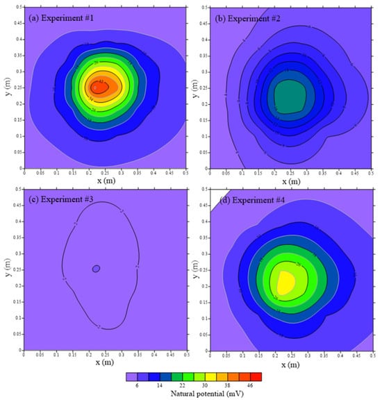
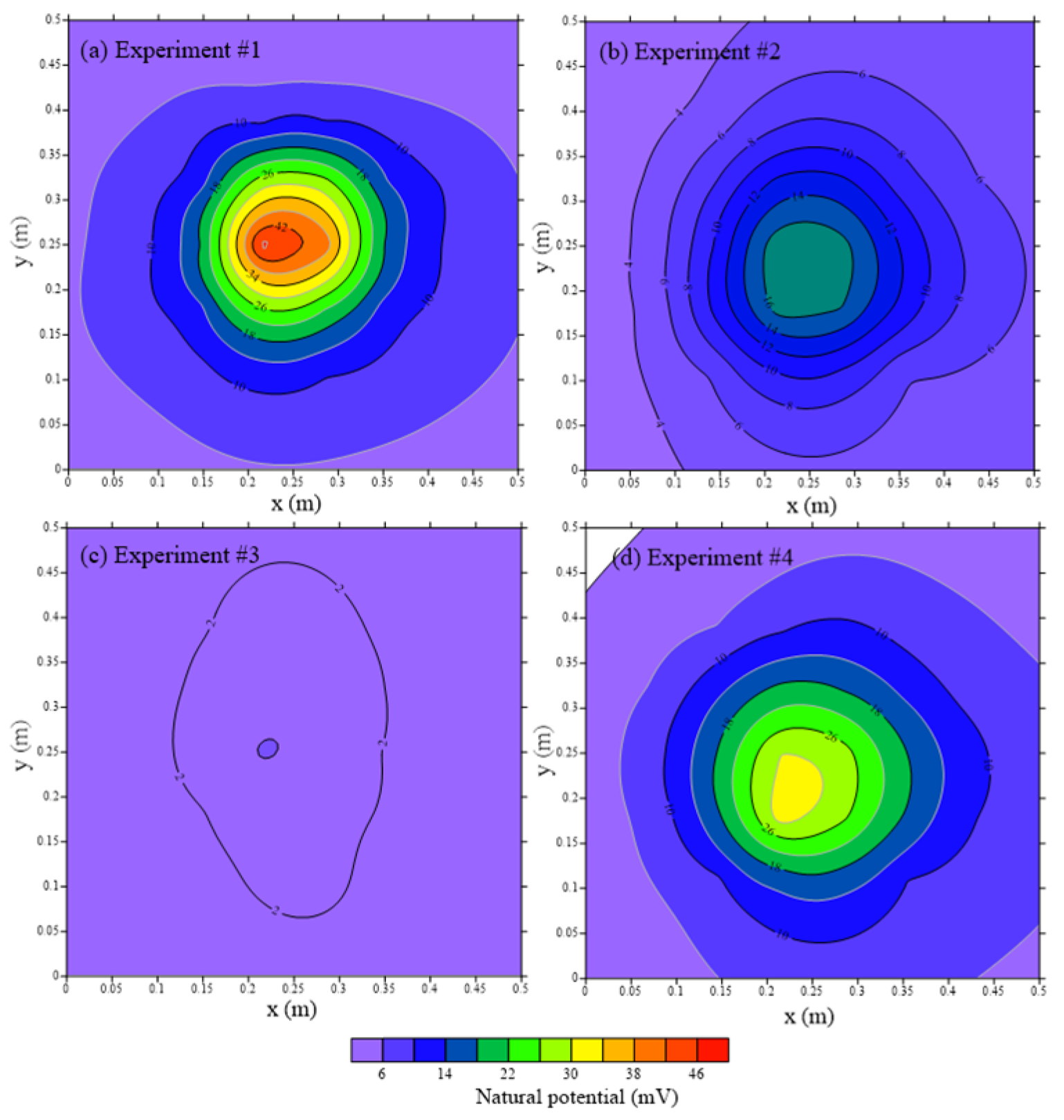
Figure 3 presents the spatial distribution of self-potential data on the upper surface of the sandbox acquired from Experiments #1 to #4. Given that the batteries are horizontally embedded at the center of the sandbox with their positive electrodes facing upward, a positive self-potential anomaly peak is observed near the center of the sandbox surface, with the anomaly amplitude decreasing radially toward the sandbox edges. In addition, the location of the maximum self-potential anomaly exhibits a slight offset relative to the horizontal center of the sandbox. This offset is attributed to local heterogeneity in the electrical conductivity of the backfilled zone, which arises from spatial variations in the compaction degree and inter-particle connectivity of the quartz sand during battery embedding and subsequent backfilling operations.

Figure 3. Self-potential contour maps of the upper surface from Experiments #1–4.

The maximum self-potential amplitudes measured on the upper surface of the sandbox are +46 mV, +16 mV, +4 mV, and +30 mV for Experiments #1 to #4, respectively. For tests with an identical number of embedded batteries, the positive self-potential anomaly amplitude detected on the surface decreases monotonically with increasing burial depth. This trend is attributed to the attenuation and diffusion of the battery-induced electric field within the conductive porous medium (quartz sand), which weakens the field’s influence on the upper surface as the source depth increases. In addition, the maximum anomaly amplitudes obtained from Experiment #2 and Experiment #4—conducted at the same battery burial depth—show an approximately 2-fold difference. This is consistent with the proportional increase in the number of embedded batteries between the two tests, confirming a positive correlation between the number of battery sources and the magnitude of surface self-potential anomalies. As the number of batteries increases, the electric fields generated by individual sources superimpose and constructively amplify, producing stronger self-potential anomalies and correspondingly higher self-potential values detected on the sandbox surface.

2.4. Self-Potential Anomaly of the Burning Coal Experiment

Self-potential anomalies from actual coal burning differ markedly from ideal point-source signals from preceding battery experiments. Experiment #5 simulated underground coal fire using a pre-ignited coal specimen embedded at the sandbox center, with self-potential data acquired at 10 min intervals (0–30 min post-ignition) to analyze electric field evolution across different combustion stages.

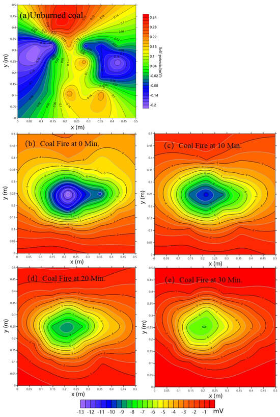
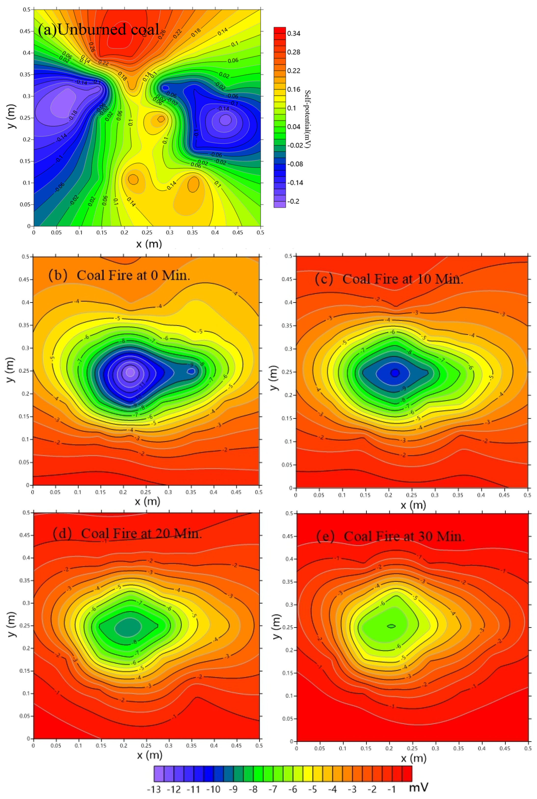
As shown in Figure 4a, after unburned coal was buried at the center of the sandbox, the self-potential measured exhibited a uniform distribution, indicating that the unburned coal did not generate any abnormalities in the natural electric field. Figure 4b shows the self-potential distribution obtained immediately after introducing burning coal into the experiment. It can be found that a negative self-potential anomaly, centered around the coal’s position, was observed on the sandbox surface, with the maximum negative anomaly reaching −13 mV. As the oxygen supply diminished, the coal combustion gradually subsided, leading to a corresponding attenuation of the negative anomaly. At 10 and 20 min, the maximum self-potential anomalies detected were −10.2 mV and −9 mV, respectively. Additionally, a slight horizontal displacement of the maximum negative anomaly from the center of the coal combustion area was observed, which was caused by variations in the compaction and overall connectivity of the quartz sand during the coal burial process. This experiment demonstrates that coal combustion at different stages can induce both positive and negative self-potential anomalies on the sandbox surface, which may be attributed to the self-potential field induced by coal fire combustion and the dipole distribution characteristics of the self-potential field.

Figure 4. Self-potential contour plots of unburned and burned coal at different stages in Experiment #5. (a) Unburned coal. (b) Coal fire at 0 min. (c) Coal fire at 10 min. (d) Coal fire at 20 min. (e) Coal fire at 30 min.

3. Test of the Inversion Algorithm

3.1. Numerical Model Settings

The surface self-potential distribution exhibits an intrinsic physical correlation with the underground source current density induced by coal burning. The spatial location of the underground coal fire source can be accurately localized by inverting the measured self-potential data, with the Poisson equation adopted as the governing equation of the self-potential field. Prior to the inversion procedure, the forward kernel matrix corresponding to the numerical model setup must be constructed [41]. Notably, the self-potential field is strongly modulated by the spatial distribution of subsurface electrical conductivity, which must be explicitly incorporated into the forward calculation of the kernel matrix [42]. After the kernel matrix is constructed in this study, the direct inversion method for cost function minimization proposed by Hansen [43] is adopted to solve for the optimal model parameters.

To further improve the depth resolution and numerical stability of the inversion results, depth weighting and the minimum support functional are introduced into the inversion framework. This iterative inversion strategy enables compact focusing of the source current density distribution, balances the data fitting residual and regularization constraints, and thus achieves high-precision 3D localization of underground coal fire sources.

To verify the applicability and robustness of the 3D iterative compact inversion algorithm used in this study across both laboratory-controlled conditions and field-scale engineering scenarios, two numerical models with distinct physical scales are constructed using the COMSOL Multiphysics 5.0 finite element analysis software. The laboratory-scale small model (hereinafter referred to as Model A) and field-scale large model (hereinafter referred to as Model B) are set with dimensions (length × width × height) of 50 cm × 50 cm × 44 cm and 320 m × 220 m × 80 m, respectively. The mesh element sizes in the core anomaly region of Model A and Model B are set to 3.5 cm × 5 cm × 5 cm (0.035 m × 0.05 m × 0.05 m) and 10 m × 25 m × 10 m, respectively.

Considering that the high temperature of coal spontaneous combustion causes complete evaporation of pore water in the surrounding strata, which eliminates the streaming potential (the primary self-potential component induced by subsurface fluid flow), the initial background self-potential of the entire computational domain is set to 0 V for both models. For Model A, to match the boundary conditions of the sandbox experiment, a constant charge density is assigned across the full domain, with the top surface, lateral sides, and bottom base all set as electrically insulating boundaries. For Model B, which replicates actual underground coal fire scenarios in natural strata, a constant charge density is similarly assigned across the entire domain; only the ground surface is set as an electrically insulating boundary, while the lateral sides and bottom base are configured as grounded infinite extension boundaries to reproduce the semi-infinite space characteristics of real geological formations. In the core region of both models, a point electric dipole (defined as a vector point source current density) is embedded at the center of the core anomaly region to simulate the current source induced by an underground coal fire, with a pre-defined vector source current density assigned to the dipole.

In line with the fixed reference point measurement method adopted in the sandbox experiment, the reference electrode for self-potential measurement is positioned along the grid edge of the upper surface of the core anomaly region for both models, to mitigate the interference of reference potential drift and boundary effects on the relative self-potential values measured at each measurement point.

The measurement point layout of Model A is completely consistent with the sandbox experimental scheme detailed in Section 2.2, yielding a total of 46 measurement points. For the field-scale Model B, five parallel rows of measurement points (survey lines) are arranged on the upper surface of the model, with a spacing of 50 m between adjacent survey lines. Measurement points along each survey line are deployed at an interval of 5 m, yielding a final total of 154 measurement points for the model. For each measurement point, the corresponding grid number and core node number in the finite element model are recorded to support subsequent self-potential data extraction and inversion calculation. Non-uniform mesh division is implemented for both models. Specifically, the sweeping and mapping meshing methods are adopted to generate refined mesh elements in the core source region and relatively coarse mesh in the peripheral far-field region, which effectively balances the numerical calculation accuracy and computational efficiency of the forward simulation.

3.2. Self-Validation of the 3D Inversion Algorithm

To verify the validity and reliability of the 3D iterative compact inversion algorithm used in this study, numerical simulation tests are carried out based on the two numerical models established above. For Model A, the vector source current density J_s is embedded at the geometric center of the model’s core domain (coordinates: x = 0.25 m, y = 0.25 m, z = 0.22 m), with a magnitude of 0.5 A·m⁻² along the positive direction of the Z-axis (i.e., J_x = 0 A·m⁻², J_y = 0 A·m⁻², J_z = +0.5 A·m⁻²). For Model B, the vector source current density J_s is positioned at the geometric center of the model’s core domain (coordinates: x = 160 m, y = 110 m, z = −40 m, where the negative Z-value denotes burial depth below the ground surface), with a magnitude of 5000 A·m⁻² along the positive direction of the Z-axis (i.e., J_x = 0 A·m⁻², J_y = 0 A·m⁻², J_z = +5000 A·m⁻²).

The subsurface resistivity distribution is an essential prerequisite for self-potential inversion and forward kernel matrix calculation. To this end, we assume a uniform and constant resistivity distribution within the computational domain for both models. The resistivity values are set to match the actual physical properties of the corresponding media: 48.7 Ωm for Model A (consistent with the measured resistivity of wet quartz sand in the sandbox experiment) and 120 Ωm for Model B (matching the typical resistivity of field coal-bearing strata). The above resistivity parameters are assigned to the model files to support the construction of the forward kernel matrix.

The self-potential distribution at each measurement point is obtained via joint numerical forward simulation using MATLAB R2013a and COMSOL Multiphysics 5.0. Subsequently, the acquired self-potential distribution data are inverted using the established resistivity model file to reconstruct the spatial distribution of the underground current sources. The inversion results are finally compared with the preset source current density in terms of spatial location and magnitude to quantitatively verify the inversion performance of the proposed algorithm.

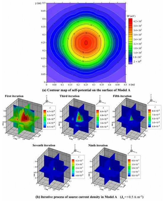
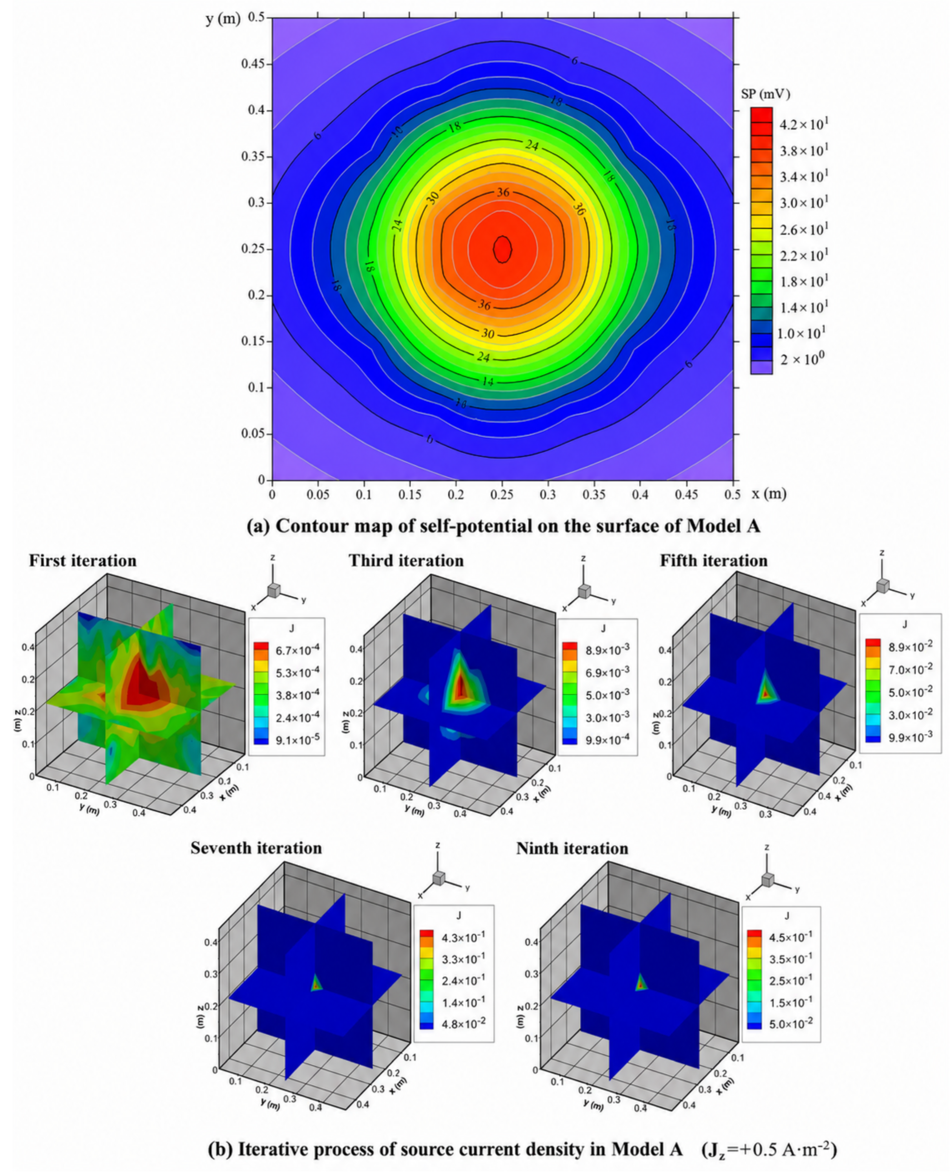
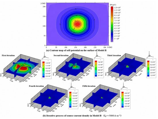
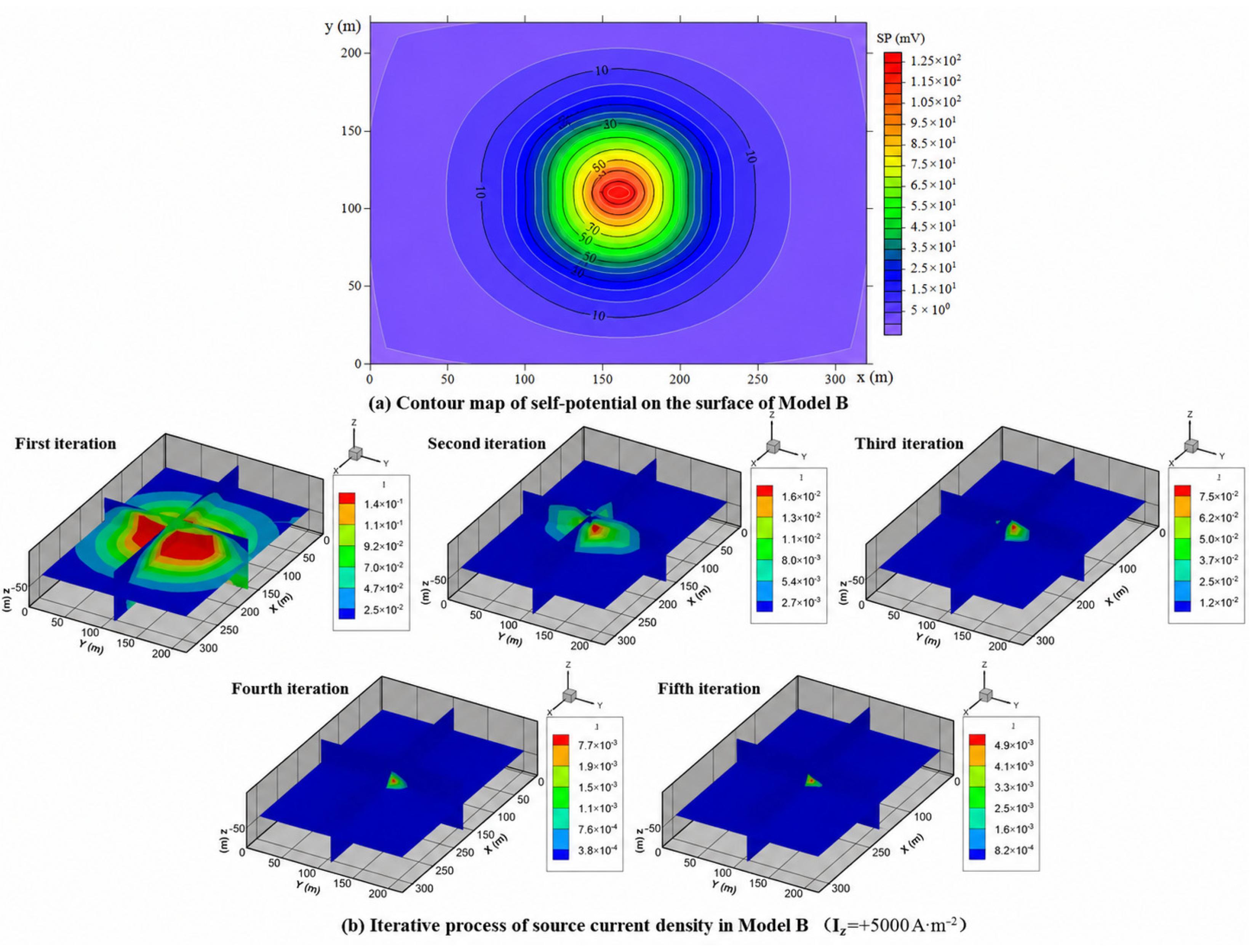
As shown in Figure 5a and Figure 6a, the Z-component of the source current density (J_z) is set at the geometric center of the two models during forward modeling, with preset values of +0.5 A·m⁻² for Model A and +5000 A·m⁻² for Model B. Positive self-potential anomalies are observed at the center of the upper surface of both models, with maximum amplitudes of +44 mV (Model A) and +130 mV (Model B), respectively. The amplitude of the self-potential anomalies decreases radially from the center to the periphery, with a gradual attenuation of the anomaly intensity. This distribution pattern is attributed to the positive Z-axis orientation of the source current density vector. With the vector source located at the horizontal center of both models, the maximum self-potential anomaly is concentrated directly above the source, i.e., at the center of the model upper surface.

Figure 5. Forward and inversion verification results of Model A with a preset source current density of +0.5 A·m⁻². (a) Contour map of self-potential on the surface of Model A. (b) Iterative process of source current density in Model A (J_z = +0.5 A·m⁻²).

Figure 6. Forward and inversion verification results of Model B with a preset source current density of +5000 A·m⁻². (a) Contour map of self-potential on the surface of Model B. (b) Iterative process of source current density in Model B (J_z = +0.5 A·m⁻²).

Figure 5b and Figure 6b present the iterative compact focusing process of the source current density during inversion for Model A and Model B, respectively. The inversion results show that the position of the converged current source gradually approaches the preset true source position as the number of iterations increases. For Model A, the source current density converges to the target value after nine iterations, while Model B achieves convergence after five iterations, with the converged source positions accurately localized to the preset true source locations. The final inversion results yield compact source current density values of 0.45 A·m⁻² (Model A) and 4900 A·m⁻² (Model B), which are in agreement with the preset true values of 0.5 A·m⁻² and 5000 A·m⁻², respectively. These results demonstrate that the proposed inversion algorithm can accurately reconstruct the distribution of self-potential source current density and achieve high-precision localization of underground self-potential current sources.

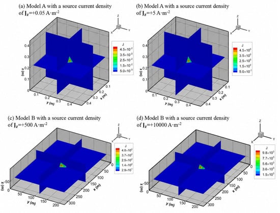
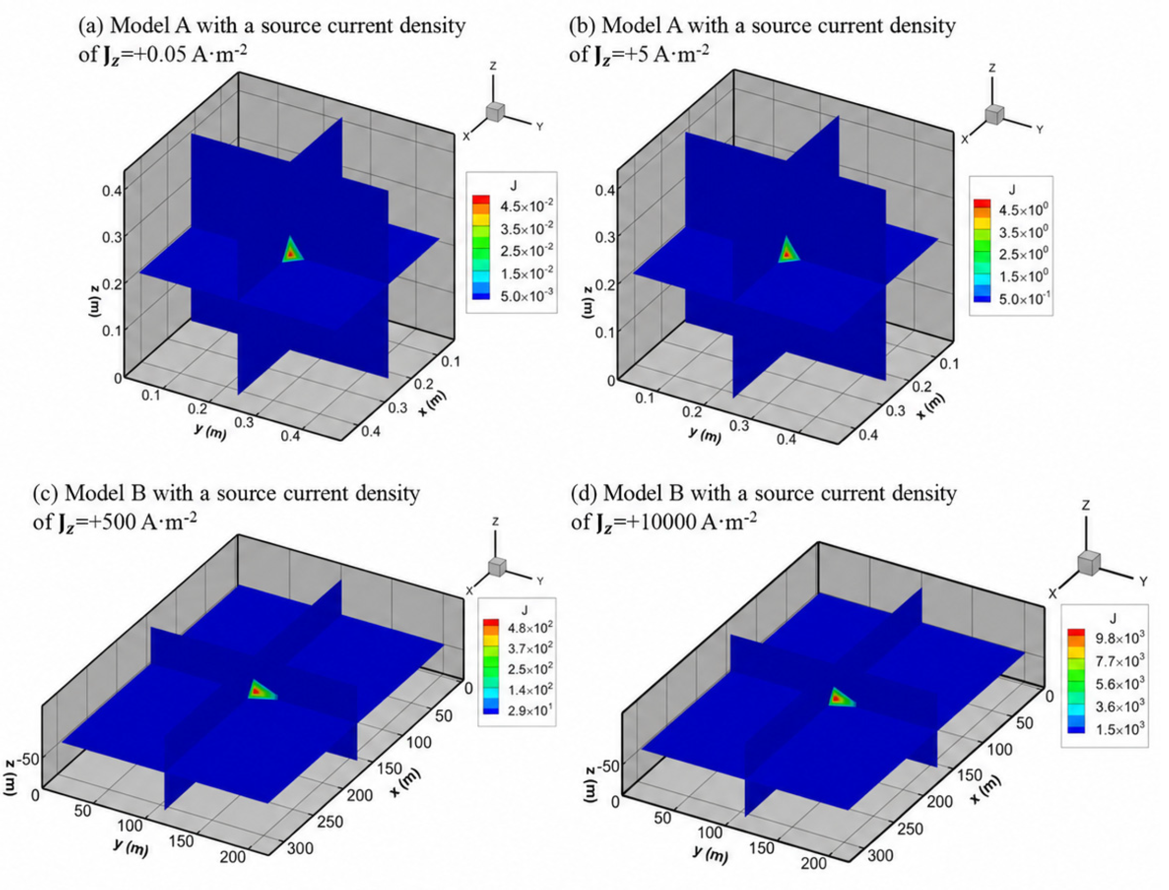
To further verify the adaptability of the proposed 3D iterative compact inversion algorithm to source current densities across a wide range of magnitudes, we design a series of numerical tests with preset source current densities spanning multiple orders of magnitude for both Model A and Model B (Figure 7). The inversion results show that the source current density undergoes progressive compact focusing during the iterative process, and the converged source is ultimately accurately localized to the preset true position for all test cases.

Figure 7. Inversion results of models A and B with different magnitudes of source current densities. (a) Model A with a source current density of J_z = +0.05 A·m⁻². (b) Model A with a source current density of J_z = +5 A·m⁻². (c) Model A with a source current density of J_z = +500 A·m⁻². (d) Model A with a source current density of J_z = +10,000 A·m⁻².

The quantitative comparison of the inversion results and preset true values is as follows: For Model A, when the preset Z-component of the source current density is J_z = +0.05 A·m⁻², the inverted value is +0.045 A·m⁻²; when the preset J_z = +5 A·m⁻², the inverted value is +4.5 A·m⁻². For Model B, when the preset J_z = +500 A·m⁻², the inverted value is +480 A·m⁻²; when the preset J_z = +10,000 A·m⁻², the inverted value is +9800 A·m⁻². All test results show that the inverted source current density is in agreement with the preset true value, with a relative error of less than 10% across all magnitude ranges. These findings demonstrate that the algorithm can achieve accurate inversion of source current densities spanning multiple orders of magnitude, and is applicable to both laboratory-scale physical simulation experiments and field-scale underground self-potential anomaly investigations.

3.3. Validation of Electric Dipole Sources

During the spontaneous combustion of underground coal seams, intense coal–oxygen chemical reactions induce charge separation and accumulation within the combustion-affected zone. The resulting spatial charge distribution governs the intrinsic characteristics of the associated electric field. An asymmetric charge distribution generates a monopole electric field, whereas a symmetric charge distribution predominantly forms a dipole electric field. These characteristic electric field distribution patterns are intrinsically coupled with the initiation and propagation of coal fires, providing a physical basis for predicting fire development trends. Therefore, continuous monitoring of the electric field distribution around burning coal seams provides a robust, non-destructive self-potential method for underground coal fire detection and early warning.

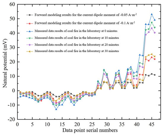
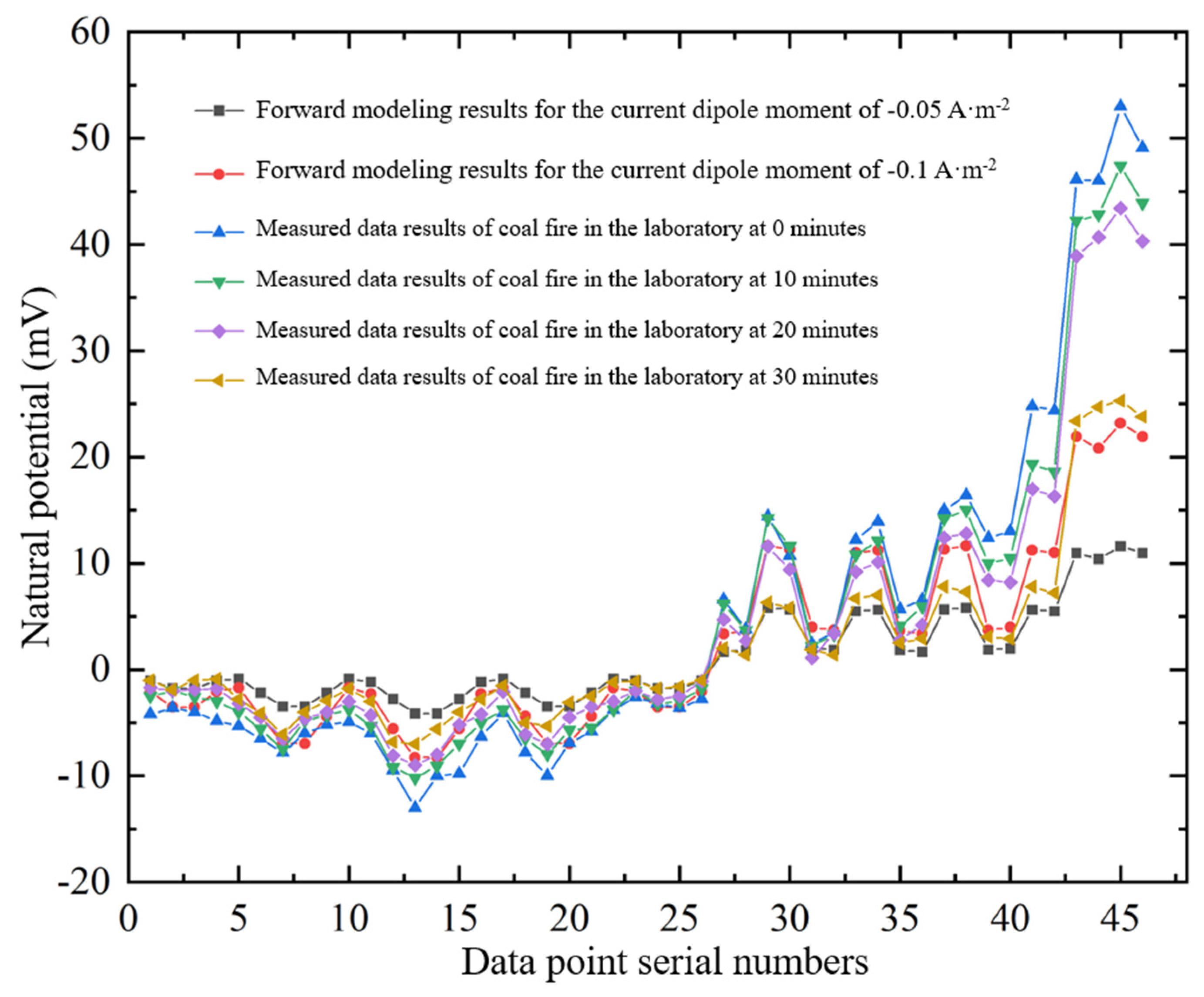
Although 46 measurement points are acquired across the upper surface, lateral sides and bottom of the sandbox in this study, this spatial sampling density is insufficient for high-precision 3D reconstruction of the full self-potential electric field distribution. To address this limitation, we conducted forward numerical simulations of a dipole source model, and compared the forward results with the experimentally measured data to characterize the electric field distribution patterns induced by coal spontaneous combustion. Consistent with the geometric and physical parameters of the sandbox experiment detailed in Section 2, forward simulations are carried out by setting appropriate dipole source magnitudes and orientations. In the forward model, the Z-component of the source current density (J_z) is oriented along the negative Z-axis, with magnitudes set to 0.05 A·m⁻² and 0.1 A·m⁻², respectively. Subsequently, the forward simulation results are compared with the laboratory-measured data to verify whether the self-potential response of the coal fire matches the theoretical dipole distribution pattern.

Figure 8 shows the comparison between the forward simulation results and the measured self-potential data at each measurement point for different coal combustion stages. The results show that the overall spatial distribution pattern of the self-potential field induced by the coal fire in the sandbox remains generally consistent across different combustion stages. As the coal fire gradually extinguishes, the amplitude of the negative self-potential anomaly on the upper surface of the sandbox (measured at points 1–26) decreases progressively. Meanwhile, positive self-potential anomalies are observed on the lateral sides and bottom of the sandbox (measured at points 27–46), with the corresponding self-potential amplitudes also decaying over time. The laboratory-measured self-potential data for different coal combustion stages are in agreement with the forward simulation curves, particularly for the cases with J_z = −0.05 A·m⁻² and J_z = −0.1 A·m⁻². This finding confirms that the self-potential field induced by underground coal spontaneous combustion presents a typical dipole distribution pattern, which further indicates that the charge distribution in the coal combustion zone has a certain degree of spatial symmetry. This conclusion is consistent with the dipole self-potential anomaly phenomenon observed by Karaoulis et al. in the Lewis coal fire area of the United States [16]. Our team also observed the same dipole self-potential anomaly phenomenon in the Heifeng No. 9 coal fire area in China [34], verifying the dipole characteristics of self-potential anomalies in the fire area.

Figure 8. Comparison of forward modeling results and measured self-potential data of coal fire in the laboratory.

4. Experimental Data Inversion

In this section, the 3D iterative compact inversion algorithm is applied to invert the self-potential data acquired from the sandbox experiments, in which batteries and pre-ignited coal samples are adopted as artificial current sources. We achieve high-precision 3D localization of the underground current sources, and further analyze the spatial and temporal variation characteristics of the source parameters.

4.1. Inversion of Self-Potential Data from Battery Experiments

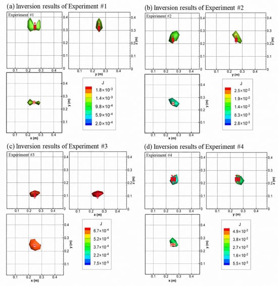
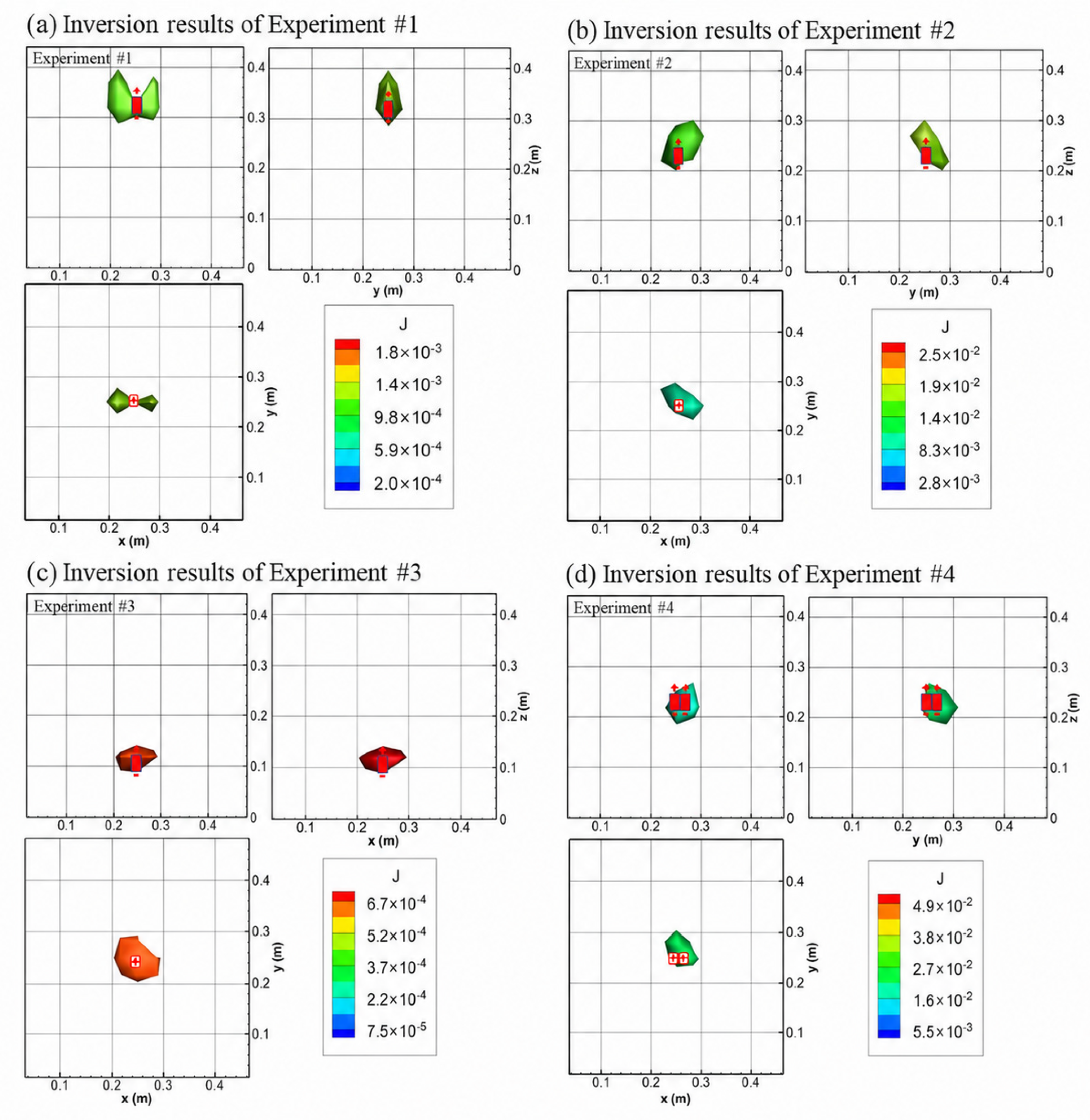
Figure 9 presents the results of the iterative compact inversion for Experiments #1–#4. The red rectangles marked with positive and negative polarities in the figure denote the pre-defined embedded positions of the batteries inside the sandbox. Comparison between the inversion outputs and the marked reference positions shows that the inverted current sources are in agreement with the actual embedded depths of the batteries, which validates the effectiveness of the adopted inversion algorithm for accurate reconstruction of the current source distribution from the measured self-potential data.

Figure 9. Self-potential inversion results of Experiments #1–4. (a) Inversion results of Experiment #1. (b) Inversion results of Experiment #2. (c) Inversion results of Experiment #3. (d) Inversion results of Experiment #4.

The supplementary self-potential measurements acquired from the side walls and bottom boundary of the sandbox markedly improve the accuracy of source depth localization, enabling high-precision inversion of current sources from the measured self-potential data. Quantitative comparison of the inversion results in Figure 9b,d reveals that, with an identical number of iterations, the inverted source current density in Experiment #4 (5.1 A·m⁻²) is approximately twice that in Experiment #2 (2.6 A·m⁻²). This finding further corroborates the superposition effect of electric fields generated by multiple battery sources, which is consistent with the self-potential amplitude variation law identified in the preceding analysis.

4.2. Inversion of Self-Potential Data from Burning Coal Experiment

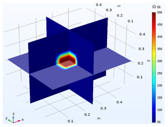
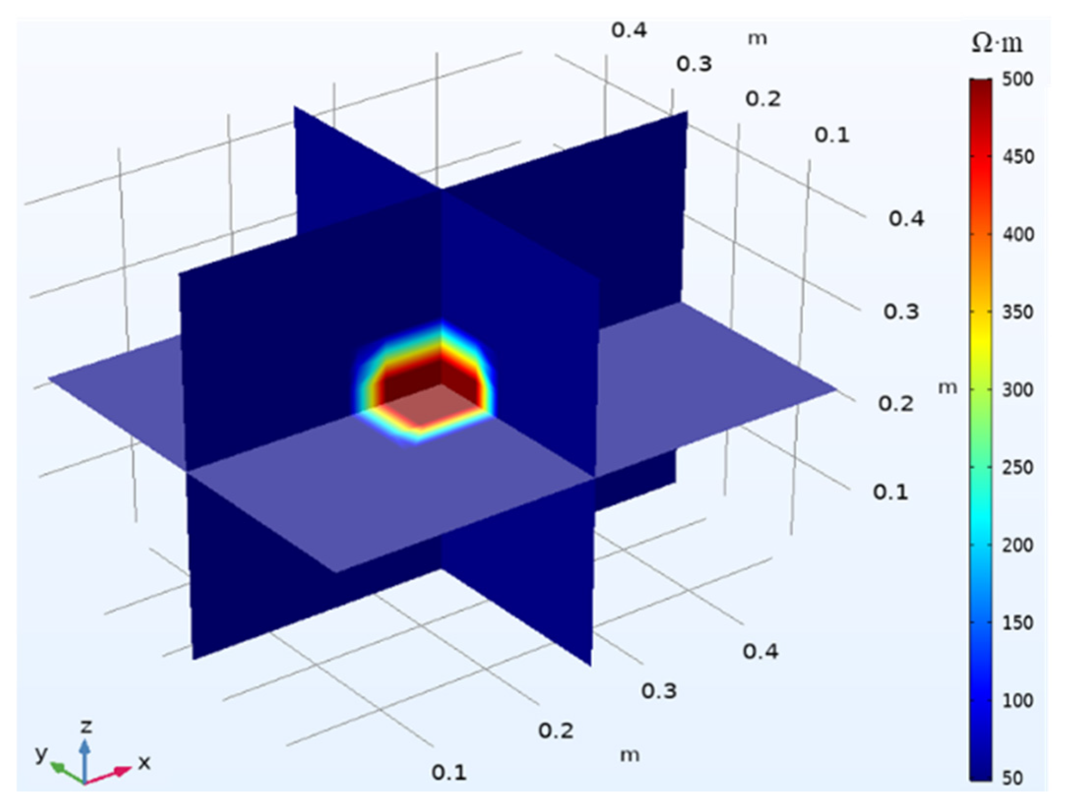
To compare the current source distribution with the actual position of the burning coal, iterative inversion of self-potential data at different stages of the coal fire in the laboratory is conducted. Considering the resistivity differences between burned and unburned coal, it is necessary to set the unburned coal area to a lower resistivity value compared to the burned coal area. In this study, the resistivity of the burned coal region is set to 500 Ωm (as shown in Figure 10).

Figure 10. Resistivity distribution diagram for burning coal sandbox experiment in Experiment #5.

In order to analyze the difference between the source current density distribution and the actual burning coal location, the resistivity distribution file is incorporated into the model for kernel matrix calculation. Subsequently, the 3D iterative compact inversion is performed based on the self-potential data measured at different combustion stages of the burning coal.

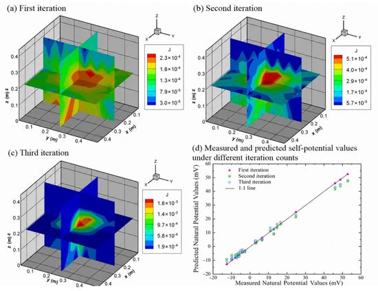
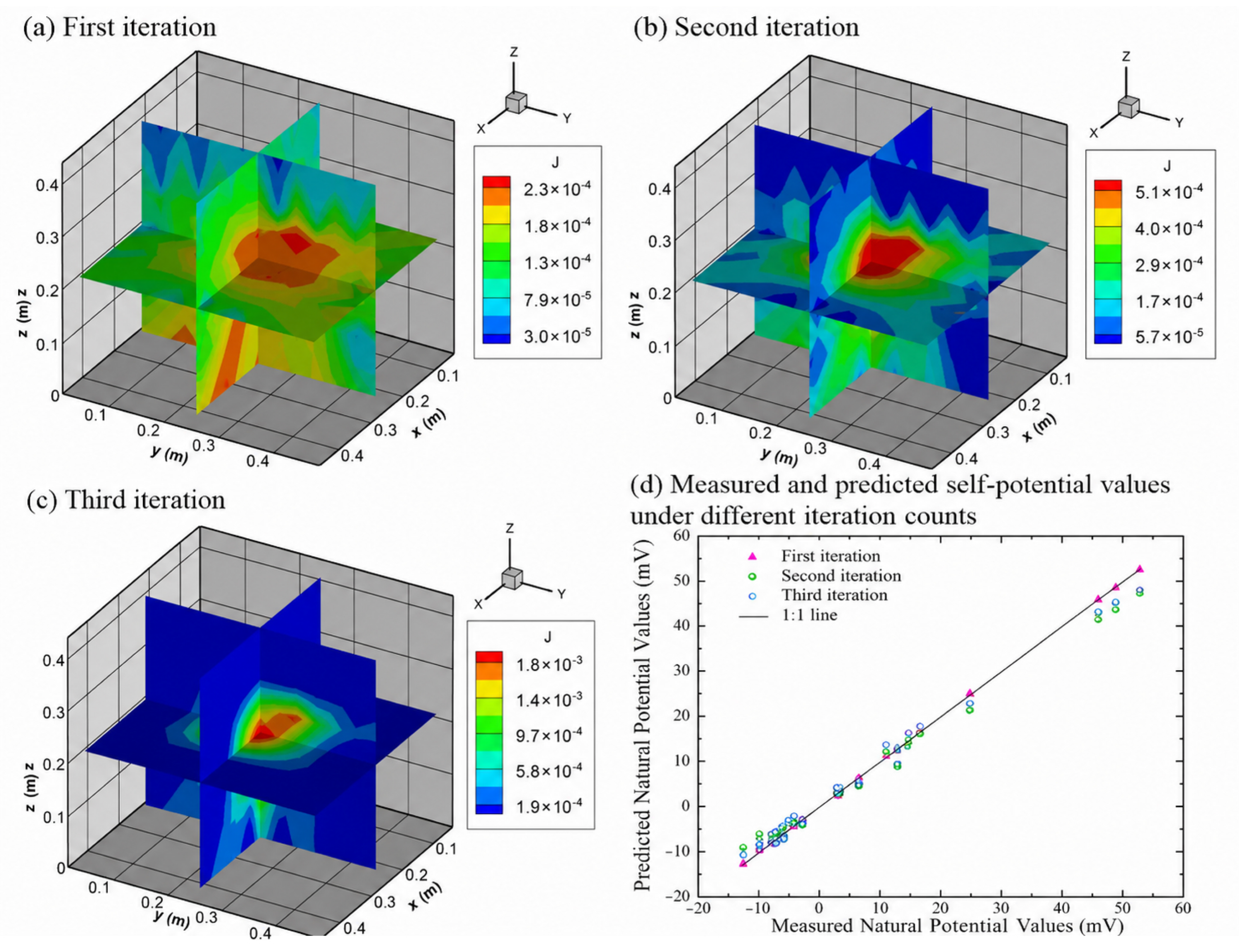
Figure 11a–c show the iterative compact focusing inversion process of the coal fire source current density at 0 min post-ignition (Iterations 1 to 3). During the inversion procedure, the spatial distribution of the source current density undergoes progressive compact focusing: the peak value of the source current density increases from 2.45 × 10⁻⁴ A·m⁻² in the first iteration to 5.36 × 10⁻⁴ A·m⁻² in the second iteration, and further increases to 1.90 × 10⁻³ A·m⁻² in the third iteration. After three iterations, the source current density distribution is sufficiently compact to accurately delineate the spatial range of the subsurface burning coal.

Figure 11. Iterative compact inversion process of coal fire source current density at 0 min post-ignition, and comparison between measured and predicted self-potential data at different iteration stages. (a) First iteration. (b) Second iteration. (c) Third iteration. (d) Measured and predicted self-potential values under different iteration counts.

Figure 11d presents the comparison between the experimentally measured self-potential data and the self-potential data predicted by the inversion model for Iterations 1 to 3. The predicted self-potential data from all three iterations are in agreement with the measured data. These results confirm that the established inversion model can accurately reproduce the observed self-potential anomalies, further verifying the reliability of the algorithm for coal fire source inversion.

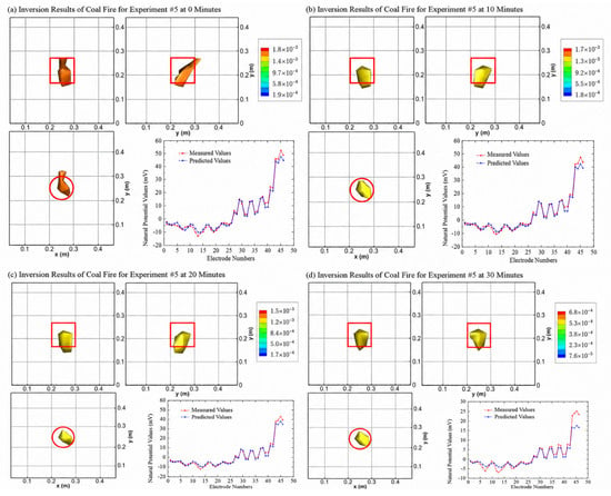
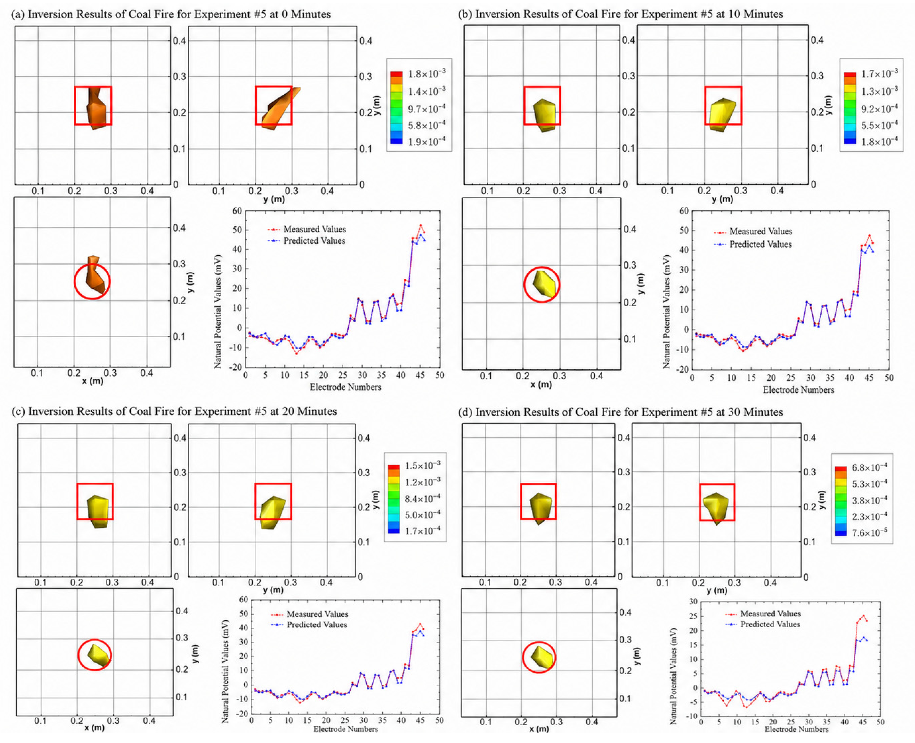
Figure 12 presents the final results of the iterative compact inversion for coal fire self-potential data at different combustion stages (0, 10, 20, and 30 min post-ignition). The spatial distribution of the inverted source current density and the delineated coal fire range are shown in the (x–y), (y–z), and (x–z) cross-sections, where the red box marks the preset true embedded position of the pre-ignited coal sample. The inversion results show that the source current density distribution at each combustion stage is concentrated at the center of the sandbox after iterative compact focusing, and is in spatial agreement with the actual coal fire position.

Figure 12. Inversion results of burning coal at different stages in Experiment #5. (a) Inversion Results of Coal Fire for Experiment #5 at 0 Minutes. (b) Inversion Results of Coal Fire for Experiment #5 at 10 Minutes. (c) Inversion Results of Coal Fire for Experiment #5 at 20 Minutes. (d) Inversion Results of Coal Fire for Experiment #5 at 30 Minutes. The red circles and rectangles denote the position of the burning coal.

Quantitative analysis shows that the peak value of the inverted source current density decreases progressively with the attenuation of the coal fire: it drops from 1.90 × 10⁻³ A·m⁻² at 0 min post-ignition to 1.80 × 10⁻³ A·m⁻² at 10 min, and further declines to 1.60 × 10⁻³ A·m⁻² at 20 min. After 30 min, the coal fire is almost extinguished, and the peak inverted current density significantly drops to 6.90 × 10⁻⁴ A·m⁻². The inversion-predicted self-potential data are in agreement with the experimentally measured data for all combustion stages. This confirms that the final iterative inversion model can accurately reproduce the self-potential field data acquired in the sandbox experiment, and further verifies the accuracy and reliability of the algorithm for underground coal fire source localization.

5. Field Application in the Sandaoba Coal Fire Area, Xinjiang

5.1. Geological Conditions of the Study Area

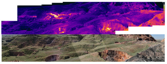
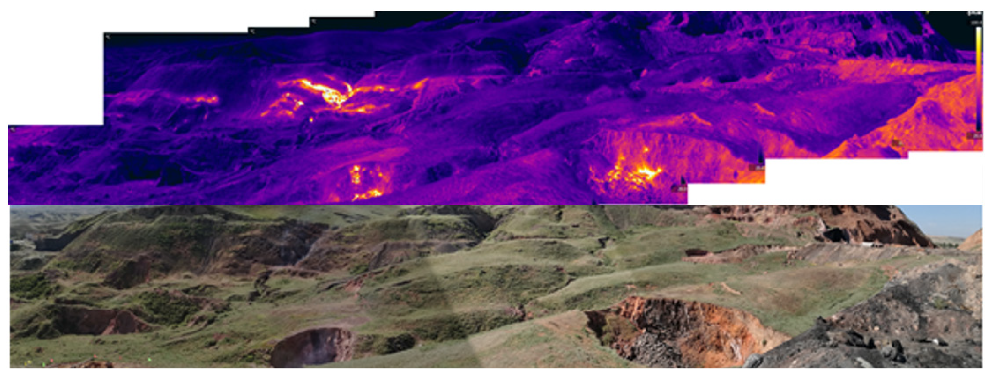
The Sandaoba Coal Fire Area is located in the eastern part of Jianquangou, Xinjiang, China. The area is dominated by a northwest-dipping monocline with a consistent strata dip angle of 79–80°, containing nine mineable coal seams with a cumulative thickness of 39.59 m. Infrared thermography results (Figure 13) indicate shallowly buried coal seams in the fire area, with typical surface features including high-temperature fire points and collapse pits. Borehole data show that the maximum combustion depth of the coal fire reaches 191 m.

Figure 13. Thermal infrared and visible light photo in the central part of the Sandaoba Coal Fire Area.

5.2. Field Survey

A comprehensive geophysical survey (including self-potential method, magnetic method, electrical resistivity tomography (ERT) and borehole temperature measurement) was carried out in the Sandaoba Coal Fire Area. A total of 55 survey lines was deployed perpendicular to the stratigraphic strike, with a cumulative line length of 25,500 m. A regular survey grid was adopted, with a fixed line spacing of 50 m and a station (measurement point) spacing of 5 m for both self-potential and magnetic data.

The self-potential data was collected using a WDJD-4 multifunctional digital direct current-induced polarization instrument (BTSK, Chongqing, China) and a pair of Cu-CuSO₄ non-polarized electrodes (used as measuring and reference electrodes, respectively). During on-site measurement, the potential drift error between the reference electrode and the measuring electrode is less than 0.1 mV, meeting the accuracy requirements. In order to ensure the reliability of self-potential anomaly data, the reference electrode was buried outside the fire area, and the measuring electrode was set up in the fire area to move and collect data point by point. To ensure good contact between the electrode and the ground, each measuring point needed to be pre-watered to reduce measurement errors. The underground resistivity data in the fire area was also collected using the WDJD-4 multifunctional instrument (BTSK, China), with an electrode spacing of 5 m. The Wenner-a array type was adopted for the survey. Due to the loose and fragmented nature of the surface in the measurement area, the grounding resistance is relatively high, and the unevenness of the ground varies greatly, which adds great difficulty to power supply and affects the reliability of the detection results. Therefore, electrolyte (salt water) was poured near the measurement point to ensure the power supply current and reduce the static errors caused by the unevenness of the ground. At the same time, the power supply voltage of the instrument was no less than 300 V and the current was about 1 A, so as to ensure sufficient signal-to-noise ratio. The least-square method is used to iteratively invert the data until the misfit becomes stable and the resistivity profile for each survey line is obtained.

The magnetic data was collected by two PMG-1 proton magnetic instruments. A magnetometer served as a daily variation observation base station, taking the Earth’s magnetic field values every 30 s to calibrate the measured magnetic anomaly data, while another magnetometer collected magnetic anomaly data by sequentially measuring points along each survey line. After the completion of the global measurement in the fire area, the magnetic field data recorded at each measurement point would be subtracted from the geomagnetic field data recorded by the daily variation observation base station at the corresponding time point to obtain the coal fire magnetic anomaly values at each measurement point.

Borehole drilling is implemented along the survey lines to determine the vertical depth range of the main burning coal seams, and to verify the geophysical anomaly interpretation results and in situ temperature measurement data.

5.3. Field Data Inversion and Analysis

Based on the field-acquired self-potential and magnetic survey data, planar contour maps of the geophysical anomalies are plotted using Surfer software 12. The anomaly results show that the coal fire area presents a multi-point scattered distribution pattern, with multiple isolated fire anomaly centers developed within the study area. To carry out high-precision 3D inversion and accurate fire range delineation, the local area covered by survey lines #38–#42 (with the most significant self-potential anomalies) is selected as the key study area. Numerical forward modeling and the 3D iterative compact inversion are performed for this target area to delineate the spatial boundary of the underground coal fire.

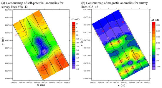
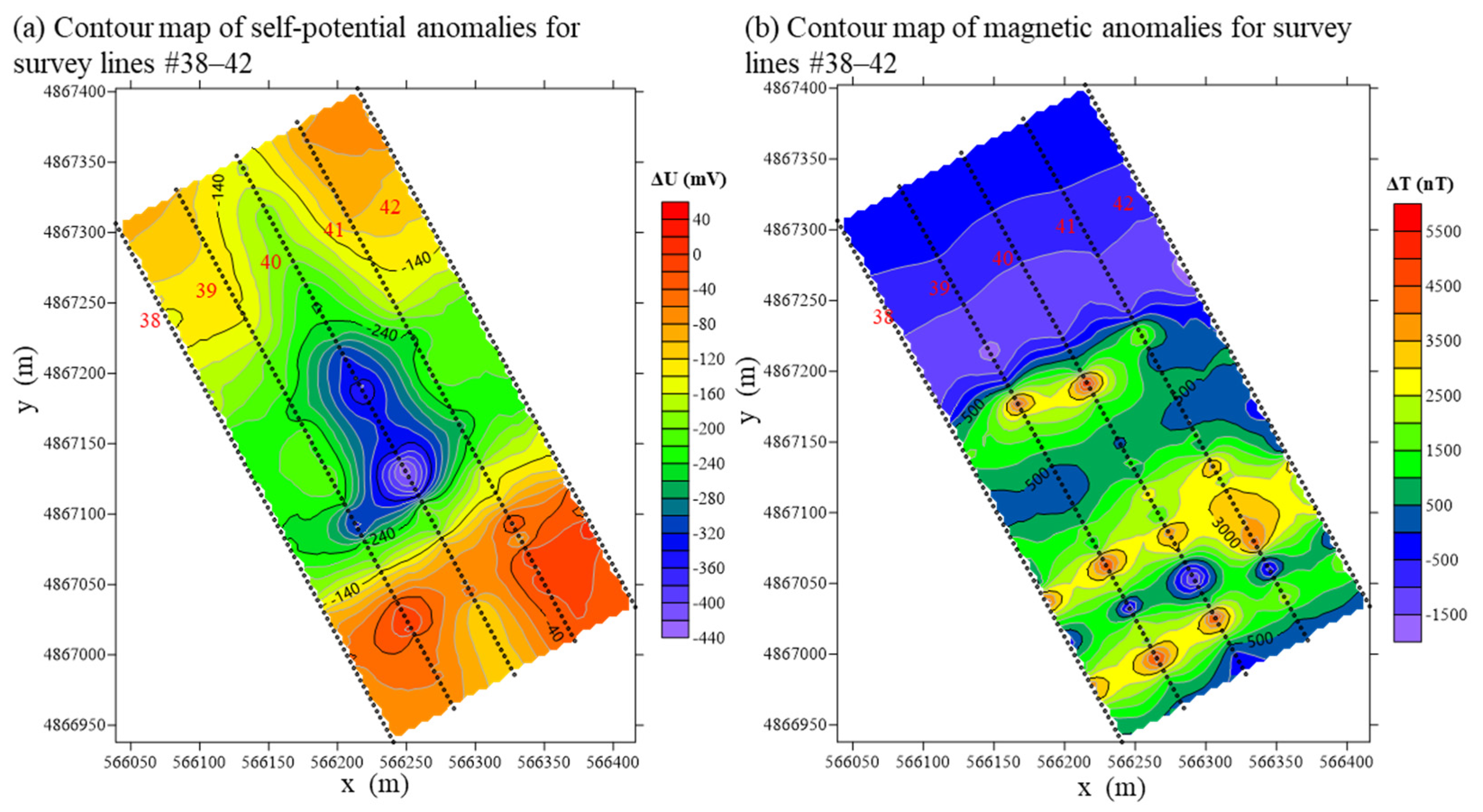
Figure 14a presents the planar distribution of self-potential anomalies in the study area. Self-potential anomalies are mainly concentrated in the central-southern part of the fire area, with a minimum anomaly value of −429 mV observed along survey line #40, marking the most prominent negative anomaly in the study area. Notably, positive self-potential anomalies are developed in the southeastern part of the study area, while negative anomalies are concentrated in the northwestern part, forming a typical dipole distribution pattern consistent with the self-potential field characteristics of underground coal fire sources revealed by the previous sandbox experiments.

Figure 14. Contour maps of self-potential and magnetic anomalies for survey lines #38–42 in the Sandaoba Coal Fire Area. (a) Contour map of self-potential anomalies for survey lines #38–42. (b) Contour map of magnetic anomalies for survey lines #38–42.To conduct high-precision 3D iterative compact inversion of the field self-potential data and delineate the underground coal fire source, a 3D numerical forward model is constructed using COMSOL Multiphysics 5.0 based on the self-potential data acquired from survey lines #38–#42. The X-axis of the model is aligned along the extension direction of the survey points (perpendicular to the stratigraphic strike), and the Y-axis is oriented parallel to the survey lines, fully consistent with the actual field survey coordinate system. The fixed reference electrode for self-potential measurement is designated at the first measurement station at the southeastern end of survey line #38, matching the field survey scheme.

Figure 14b shows the planar distribution of magnetic anomalies in the study area. Unlike the self-potential anomaly pattern, positive magnetic anomalies are dominant in the southeastern part of the fire area, with additional positive anomaly zones developed in the central and northern parts. The peak magnetic anomalies along survey lines #39–#41 reach 5240 nT, 5488 nT and 4760 nT, respectively. These high-amplitude magnetic anomalies indicate that the surrounding rocks in the fire area have undergone significant thermoremanent magnetization due to coal burning, which is a typical geophysical signature of in situ coal fires.

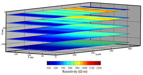
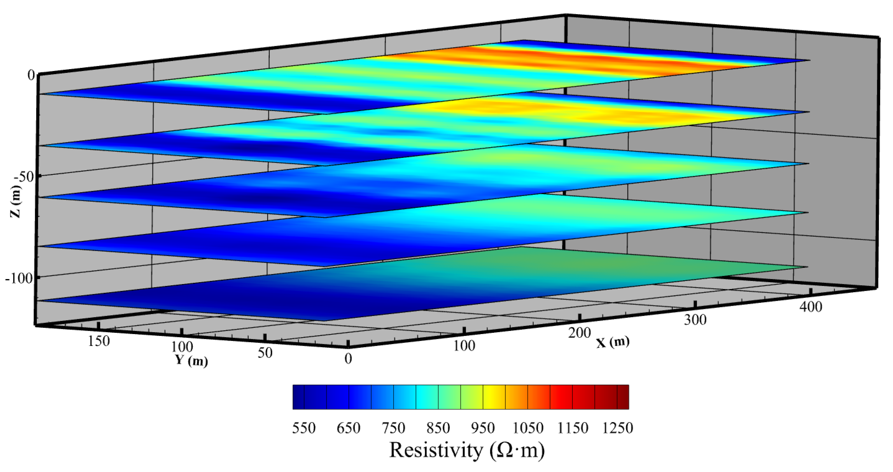
Prior to self-potential inversion, resistivity values of each stratigraphic unit are assigned to the model grid based on the electrical resistivity tomography method. The resistivity collected in the fire area is inversed by RES3D INV 2.15. Figure 15 shows the 3D resistivity distribution of survey lines #38–#42. As shown in the figure, there is not much difference in resistivity in this area (about 550 to 1250 Ωm), and the resistivity shows a significant strip-shaped increasing trend along the X-axis. The low resistivity anomaly concentration area is located at X = 0–200 m, and the resistivity change in the Y-axis direction is relatively gentle. On the west side of the study area, as the burial depth increases, the resistivity shows a significant decreasing trend, which may be related to the decrease in coal and rock resistivity caused by high temperature. The inverted resistivity model is then imported into the forward model to complete the kernel matrix calculation, consistent with the numerical simulation workflow described in the previous sections.

Figure 15. 3D resistivity distribution of survey lines #38–#42.

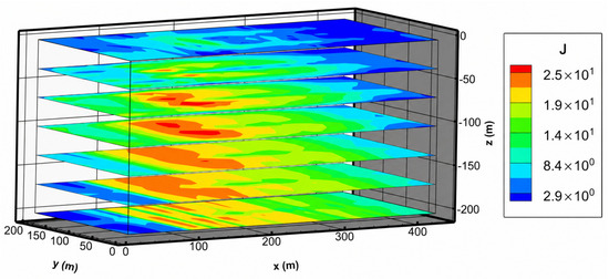
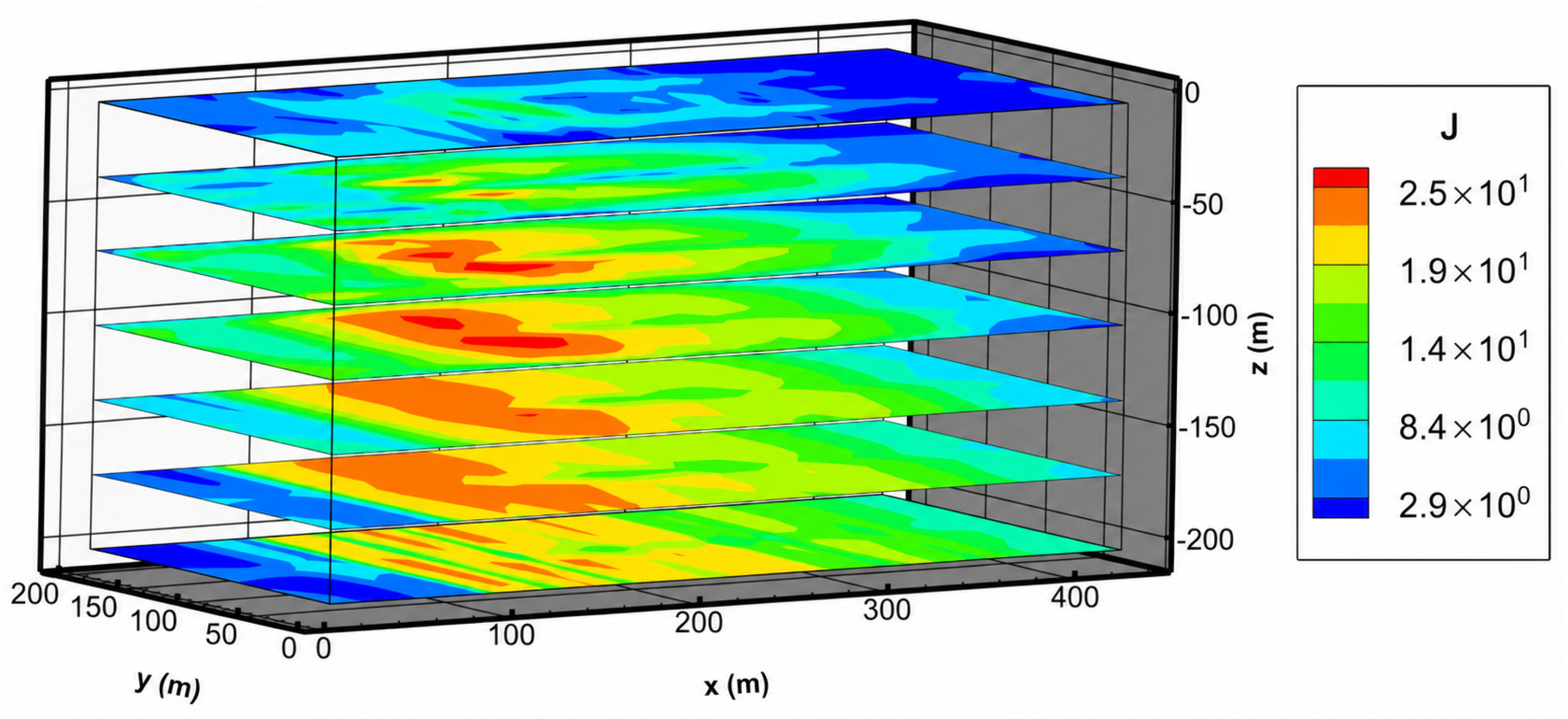
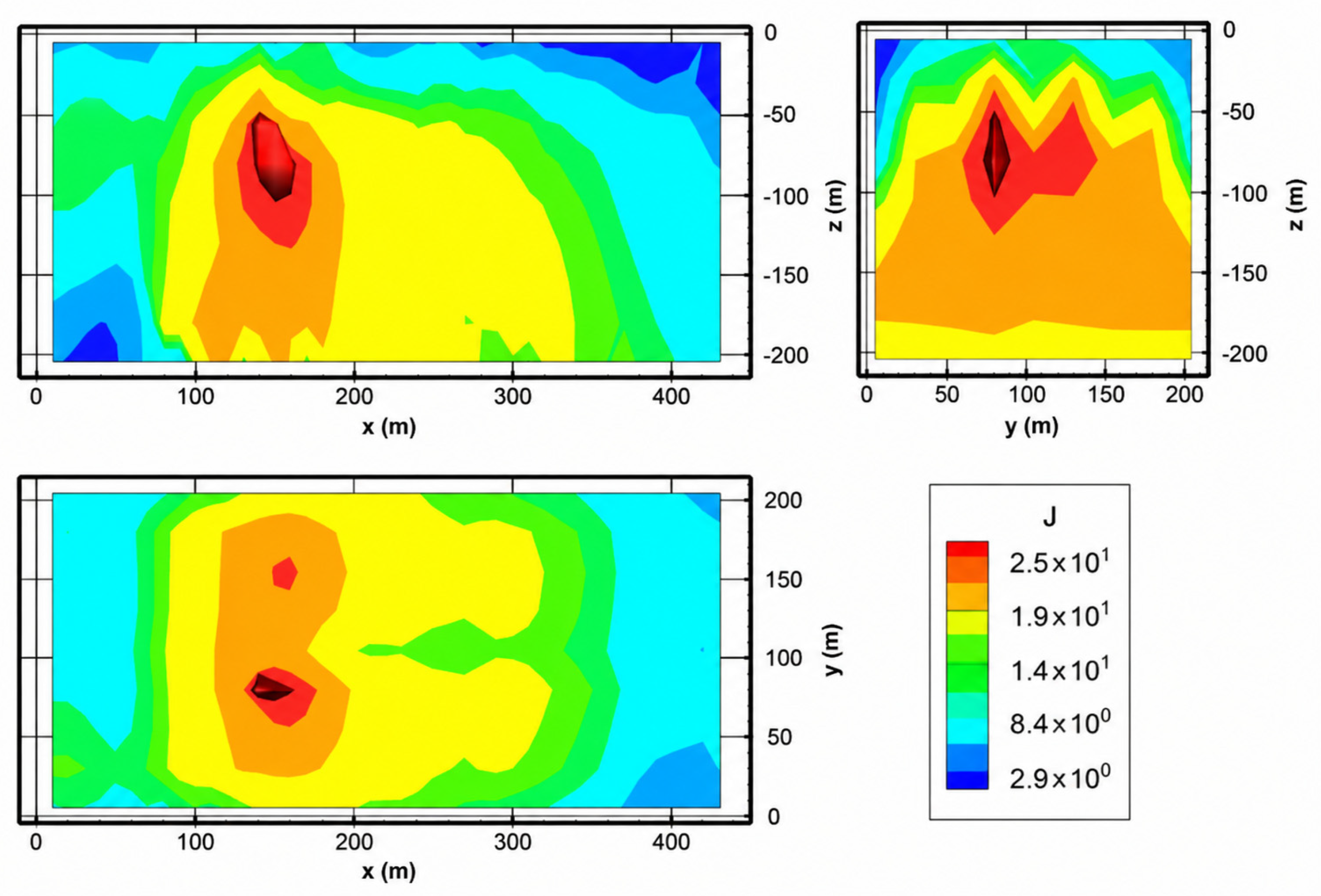
Figure 16 presents the 3D spatial distribution of the source current density obtained via the proposed iterative compact inversion algorithm. After moderate Gaussian filtering is applied to the inverted current density data to eliminate low-amplitude background noise and highlight effective fire source anomalies, a high-amplitude current source zone with a peak current density of 25 A·m⁻² is identified in the southwestern part of the model domain.

Figure 16. 3D stereogram of the coal fire source current density inversion results.

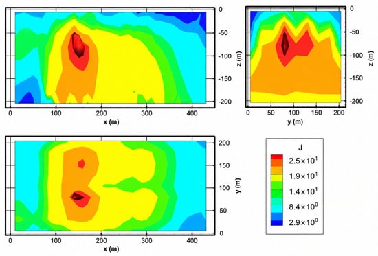
To accurately delineate the spatial boundary of the coal fire source, the inversion results are displayed in (x–y), (y–z) and (x–z) cross-sections in Figure 17. The cross-sections show that the inversion-delineated coal fire source extends horizontally from 140 m to 160 m along the X-axis and from 70 m to 90 m along the Y-axis. Vertically, the coal fire is buried at depths ranging from 40 m to 100 m below the ground surface, presenting a wide vertical distribution range consistent with the large dip angle of the coal seams in the study area. Furthermore, field borehole temperature measurement data reveal that the peak temperature (around 700 °C) is concentrated at a depth of ~80 m below the ground surface, which falls within the depth range of the coal fire delineated by the inversion results, providing independent in situ verification for the accuracy and reliability of the inversion.

Figure 17. Cross-sections of the coal fire source inversion results.

6. Conclusions

In this study, a 3D iterative compact inversion algorithm for self-potential data is used to achieve accurate 3D localization of concealed underground coal fire sources. Its performance is systematically verified through numerical simulations, laboratory sandbox experiments, and field engineering application. The core conclusions are as follows:

(1) The algorithm exhibits good robustness and inversion accuracy. By introducing depth weighting and the minimum support functional, it effectively solves the ill-posed problem of self-potential inversion, and realizes high-precision reconstruction of source current density across multiple orders of magnitude, with a relative error of less than 10% between inverted and preset true values in multi-scale numerical simulations.

(2) Laboratory experiments clarify the self-potential response mechanism of underground coal fires. Coal combustion generates a typical dipole self-potential field with distinct negative surface anomalies, whose amplitude is positively correlated with combustion intensity. The inversion results for sandbox data are highly consistent with the actual positions of artificial current sources and burning coal specimens, verifying the algorithm’s reliability under controlled conditions.

(3) Field application in the Sandaoba Coal Fire Area confirms the algorithm’s engineering practicability. The 3D inversion results successfully delineate the spatial boundary of the concealed fire source (buried at 40–100 m), which is in agreement with borehole temperature data (peak combustion temperature of ~700 °C at ~80 m depth).

References

- Liang, Y.; Yang, Y.; Guo, S.; Tian, F.; Wang, S. Combustion mechanism and control approaches of underground coal fires: A review. Int. J. Coal Sci. Technol. 2023, 10, 24. [Google Scholar] [CrossRef] [Scilit]
- Wang, T.; Wang, H.; Fang, X.; Wang, G.; Chen, Y.; Xu, Z.; Qi, Q. Research progress and visualization of underground coal fire detection methods. Environ. Sci. Pollut. Res. 2023, 30, 74671–74690. [Google Scholar] [CrossRef] [Scilit]
- Song, Z. Modelling oxygen-limited and self-sustained smoldering propagation: Underground coal fires driven by thermal buoyancy. Combust. Flame 2022, 245, 112382. [Google Scholar] [CrossRef] [Scilit]
- Song, Z.; Kuenzer, C. Coal fires in China over the last decade: A comprehensive review. Int. J. Coal Geol. 2014, 133, 72–99. [Google Scholar] [CrossRef] [Scilit]
- Shao, Z.; Jia, X.; Zhong, X.; Wang, D.; Wei, J.; Wang, Y.; Chen, L. Detection, extinguishing, and monitoring of a coal fire in Xinjiang, China. Environ. Sci. Pollut. Res. 2018, 25, 26603–26616. [Google Scholar] [CrossRef] [Scilit]
- Van Dijk, P.; Zhang, J.; Jun, W.; Kuenzer, C.; Wolf, K.-H. Assessment of the contribution of in-situ combustion of coal to greenhouse gas emission; based on a comparison of Chinese mining information to previous remote sensing estimates. Int. J. Coal Geol. 2011, 86, 108–119. [Google Scholar] [CrossRef] [Scilit]
- Kuenzer, C.; Stracher, G.B. Geomorphology of coal seam fires. Geomorphology 2012, 138, 209–222. [Google Scholar] [CrossRef] [Scilit]
- Li, F.; Li, J.; Liu, X.; Meng, X. Coal fire detection and evolution of trend analysis based on CBERS-04 thermal infrared imagery. Environ. Earth Sci. 2020, 79, 384. [Google Scholar] [CrossRef] [Scilit]
- Riyas, M.J.; Syed, T.H.; Kumar, H.; Kuenzer, C. Detecting and analyzing the evolution of subsidence due to coal fires in Jharia Coalfield, India using Sentinel-1 SAR data. Remote Sens. 2021, 13, 1521. [Google Scholar] [CrossRef] [Scilit]
- Karanam, V.; Motagh, M.; Garg, S.; Jain, K. Multi-sensor remote sensing analysis of coal fire induced land subsidence in Jharia Coalfields, Jharkhand, India. Int. J. Appl. Earth Obs. Geoinf. 2021, 102, 102439. [Google Scholar] [CrossRef] [Scilit]
- Wang, T.; Wang, Y.; Zhao, F.; Feng, H.; Liu, J.; Zhang, L.; Zhang, N.; Yuan, G.; Wang, D. A spatio-temporal temperature-based thresholding algorithm for underground coal fire detection with satellite thermal infrared and radar remote sensing. Int. J. Appl. Earth Obs. Geoinf. 2022, 110, 102805. [Google Scholar] [CrossRef] [Scilit]
- Yuan, G.; Wang, Y.; Zhao, F.; Yan, S.; Zhang, H.; Lang, F.; Hao, M.; Cao, F.; Peng, B.; Dang, L. Spatiotemporal correlation characteristics between thermal infrared remote sensing obtained surface thermal anomalies and reconstructed 4-D temperature fields of underground coal fires. IEEE Trans. Geosci. Remote 2023, 61, 1–18. [Google Scholar] [CrossRef] [Scilit]
- Chen, Y.; Suo, Z.; Li, J.; Wei, J.; Cao, F.; Sun, H.; Li, H.; Gao, Y.; Li, Q.; Yue, Y. Active–Passive remote sensing identification of underground coal fire zones with joint constraints of temperature and surface deformation time series. IEEE J. Sel. Top. Appl. Earth Obs. Remote Sens. 2023, 17, 894–915. [Google Scholar] [CrossRef] [Scilit]
- Yu, B.; She, J.; Liu, G.; Ma, D.; Zhang, R.; Zhou, Z.; Zhang, B. Coal fire identification and state assessment by integrating multitemporal thermal infrared and InSAR remote sensing data: A case study of Midong District, Urumqi, China. Isprs J. Photogramm. 2022, 190, 144–164. [Google Scholar] [CrossRef] [Scilit]
- Zhang, J.; Kuenzer, C. Thermal surface characteristics of coal fires 1 results of in-situ measurements. J. Appl. Geophys. 2007, 63, 117–134. [Google Scholar] [CrossRef] [Scilit]
- Karaoulis, M.; Revil, A.; Mao, D. Localization of a coal seam fire using combined self-potential and resistivity data. Int. J. Coal Geol. 2014, 128, 109–118. [Google Scholar] [CrossRef] [Scilit]
- Gangopadhyay, P.K.; Maathuis, B.; Van Dijk, P. ASTER-derived emissivity and coal-fire related surface temperature anomaly: A case study in Wuda, north China. Int. J. Remote Sens. 2005, 26, 5555–5571. [Google Scholar] [CrossRef] [Scilit]
- Zhang, B.; Xiao, F.; Jin, W. Burnt coal field detection via magnetic exploration. Environ. Earth Sci. 2023, 82, 160. [Google Scholar] [CrossRef] [Scilit]
- Hu, X.; Hong, H.; Dong, H.; Wu, B.; Sun, Z.; Wang, W.; Zhang, Q. Research on the application of “radon measurement-magnetic” method to detect spontaneous combustion technology in small coal mines. Coal Sci. Technol. 2025, 53, 198–208. [Google Scholar]
- Yuan, S.; Sun, Q.; Zhao, Y.; Hu, X.; Wang, S.; Ge, Z.; Chen, K. Mechanism of rock magnetic susceptibility response in coal fire zone under high-temperature environment. Acta Geophys. 2025, 73, 4323–4337. [Google Scholar] [CrossRef] [Scilit]
- Xue, S.; Dickson, B.; Wu, J. Application of 222Rn technique to locate subsurface coal heatings in Australian coal mines. Int. J. Coal Geol. 2008, 74, 139–144. [Google Scholar] [CrossRef] [Scilit]
- Zhang, Z.; Zhang, H.; Ma, T.; Li, J.; Wang, Y.; Thanh, H.V.; Ngo, I. Environmental hazards of coal fires: Fracture-driven radon anomalies and migration. Process Saf. Environ. Prot. 2025, 201, 107592. [Google Scholar] [CrossRef] [Scilit]
- Zhou, B.; Deng, C.; Hao, J.; An, B.; Wu, R. Experimental study on the mechanism of radon exhalation during coal spontaneous combustion in goaf. Tunn. Undergr. Space Technol. 2021, 113, 103776. [Google Scholar] [CrossRef] [Scilit]
- Du, B.; Liang, Y.; Tian, F. Detecting concealed fire sources in coalfield fires: An application study. Fire Saf. J. 2021, 121, 103298. [Google Scholar] [CrossRef] [Scilit]
- Kong, B.; Liu, Z.; Yao, Q. Study on the electromagnetic spectrum characteristics of underground coal fire hazardous and the detection criteria of high temperature anomaly area. Environ. Earth Sci. 2021, 80, 89. [Google Scholar] [CrossRef] [Scilit]
- Shao, Z.; Wang, D.; Wang, Y.; Zhong, X.; Tang, X.; Xi, D. Electrical resistivity of coal-bearing rocks under high temperature and the detection of coal fires using electrical resistance tomography. Geophys. J. Int. 2016, 204, 1316–1331. [Google Scholar]
- Revil, A.; Karaoulis, M.; Srivastava, S.; Byrdina, S. Thermoelectric self-potential and resistivity data localize the burning front of underground coal fires. Geophysics 2013, 78, B259–B273. [Google Scholar] [CrossRef] [Scilit]
- King, A. Cindered coal detection using transient electromagnetic methods. Geoexploration 1987, 24, 367–379. [Google Scholar] [CrossRef] [Scilit]
- Shao, Z.; Deng, R.; Zhou, T.; Cao, F.; Sun, H.; Chen, L.; Yuan, Y.; Zhong, X. 3D Localization of Coal Fires Based on Self-Potential Data: Sandbox Experiments. Pure Appl. Geophys. 2021, 178, 4583–4603. [Google Scholar] [CrossRef] [Scilit]
- Pekşen, E.; Yas, T.; Kayman, A.Y.; Özkan, C. Application of particle swarm optimization on self-potential data. J. Appl. Geophys. 2011, 75, 305–318. [Google Scholar] [CrossRef] [Scilit]
- Shao, Z.; Wang, D.; Wang, Y.; Zhong, X.; Zhang, Y.; Song, W. Experimental study of the self-potential anomaly caused by coal fires. J. Appl. Geophys. 2017, 145, 124–132. [Google Scholar] [CrossRef] [Scilit]
- Kumar, S.; Pal, S.K. Underground Coal fire Mapping Using Analysis of Self-potential (SP) Data Collected from Akashkinaree Colliery, Jharia Coalfield, India. J. Geol. Soc. India 2020, 95, 350–358. [Google Scholar] [CrossRef] [Scilit]
- Shao, Z.; Liang, Y.; Tian, F.; Song, S.; Deng, R. Constructing 3D Land Surface Temperature Model of Local Coal Fires Using UAV Thermal Images. IEEE Trans. Geosci. Remote Sens. 2022, 60, 5002309. [Google Scholar] [CrossRef] [Scilit]
- Shao, Z.; Zhang, G.; Zhou, T.; Wei, J.; Cao, F.; Zhang, Y.; Li, H.; Sun, H.; Qing, S.; Chen, T.; et al. Locating the Scope and Depth of Coal Fires Based on Magnetic and Electrical Data. Pure Appl. Geophys. 2023, 180, 3883–3900. [Google Scholar] [CrossRef] [Scilit]
- Srivardhan, V.; Pal, S.; Vaish, J.; Kumar, S.; Bharti, A.K.; Priyam, P. Particle swarm optimization inversion of self-potential data for depth estimation of coal fires over East Basuria colliery, Jharia coalfield, India. Environ. Earth Sci. 2016, 75, 688. [Google Scholar] [CrossRef] [Scilit]
- El-Kaliouby, H.M.; Al-Garni, M.A. Inversion of self-potential anomalies caused by 2D inclined sheets using neural networks. J. Geophys. Eng. Geol. 2009, 6, 29–34. [Google Scholar] [CrossRef] [Scilit]
- Göktürkler, G.; Balkaya, Ç. Inversion of self-potential anomalies caused by simple-geometry bodies using global optimization algorithms. J. Geophys. Eng. Geol. 2012, 9, 498–507. [Google Scholar] [CrossRef] [Scilit]
- Abdelrahman, E.-S.M.; Essa, K.S.; Abo-Ezz, E.R.; Sultan, M.; Sauck, W.A.; Gharieb, A.G. New least-squares algorithm for model parameters estimation using self-potential anomalies. Comput. Geosci. 2008, 34, 1569–1576. [Google Scholar] [CrossRef] [Scilit]
- Skianis, G.A.; Papadopoulos, T.; Vaiopoulos, D. Direct interpretation of self-potential anomalies produced by a vertical dipole. J. Appl. Geophys. 2006, 58, 130–143. [Google Scholar] [CrossRef] [Scilit]
- Linde, N.; Jougnot, D.; Revil, A.; Matthäi, S.; Arora, T.; Renard, D.; Doussan, C. Streaming current generation in two-phase flow conditions. Geophys. Res. Lett. 2007, 34, L03306. [Google Scholar] [CrossRef] [Scilit]
- Jardani, A.; Revil, A.; Bolève, A.; Dupont, J.-P. Three-dimensional inversion of self-potential data used to constrain the pattern of groundwater flow in geothermal fields. J. Geophys. Res. Solid Earth 2008, 113, B09204. [Google Scholar] [CrossRef] [Scilit]
- Mao, D.; Revil, A.; Hort, R.D.; Munakata-Marr, J.; Atekwana, E.A.; Kulessa, B. Resistivity and self-potential tomography applied to groundwater remediation and contaminant plumes: Sandbox and field experiments. J. Hydrol. 2015, 530, 1–14. [Google Scholar] [CrossRef] [Scilit]
- Hansen, P.C. Rank-Deficient and Discrete Ill-Posed Problems: Numerical Aspects of Linear Inversion; SIAM: Philadelphia, PA, USA, 1998. [Google Scholar]
Disclaimer/Publisher’s Note: The statements, opinions and data contained in all publications are solely those of the individual author(s) and contributor(s) and not of MDPI and/or the editor(s). MDPI and/or the editor(s) disclaim responsibility for any injury to people or property resulting from any ideas, methods, instructions or products referred to in the content. |
© 2026 by the authors. Licensee MDPI, Basel, Switzerland. This article is an open access article distributed under the terms and conditions of the Creative Commons Attribution (CC BY) license.