Input Sensitivity and Simulation Accuracy of WindNinja Wind Field Simulations in Complex Plateau Mountainous Terrain

Abstract

Near-surface wind field simulation in complex mountainous terrain is essential for predicting wildfire behavior and supporting fire risk management. WindNinja, a widely used diagnostic wind downscaling model, is strongly dependent on its initial input data; however, systematic evaluations of its input sensitivity and simulation accuracy remain limited. In this study, a representative canyon area was selected as the study site. WindNinja was driven by three types of input data: local meteorological station observations, national meteorological station observations, and ERA5-Land reanalysis data. Two indices—the Wind Forcing Intensity (WFI) index and the Thermal Forcing Intensity (TFI) index—were constructed to classify weather-forcing scenarios and evaluate simulation accuracy under different conditions. The results show that differences in the statistical characteristics of the initial wind sources produce pronounced sensitivity in WindNinja simulations. Simulations driven by local meteorological observations generally overestimate wind speed, whereas ERA5-Land-driven simulations systematically underestimate wind speed, with national-station results falling between these two cases. Simulation accuracy varies with terrain position: wind direction errors dominate in valleys, whereas wind speed errors dominate on ridges and hilltops. Weather background conditions significantly influence simulation accuracy. Wind forcing intensity dominates the magnitude and dispersion of simulation errors, while strong thermal forcing leads to an overall decline in simulation accuracy and stability. These findings highlight the sensitivity of WindNinja to initial wind sources and weather background conditions in complex terrain and provide guidance for its application and uncertainty control in wildfire behavior modeling.

1. Introduction

Wildfire occurrence and spread are highly sensitive to near-surface wind conditions, which directly influence the direction, rate of spread, and intensity of fire behavior [1]. In complex mountainous environments, terrain variations can substantially modify near-surface airflow through blocking, channeling, and acceleration effects, producing localized wind acceleration, directional deflection, and enhanced turbulence [2]. These microscale wind field variations are often difficult to accurately capture using conventional meteorological observations or mesoscale numerical models [3,4]. Yet, they constitute the key driving forces behind the onset of eruptive fires, fire whirls, and spot fires [5,6].

Because observational coverage in complex terrain is often sparse, high-resolution wind fields are commonly reconstructed through numerical downscaling methods. Diagnostic wind models are widely used in wildfire research and operational applications because of their computational efficiency and ease of implementation [7]. Among these models, WindNinja has become one of the most widely used tools for downscaling near-surface wind fields and has been integrated into several wildfire behavior modeling systems, including FlamMap and FARSITE [8,9]. The accuracy of any model must be rigorously validated using observational data. However, in complex terrain, the scarcity of high-quality observations remains a major limitation for model evaluation and improvement. Existing validation studies of WindNinja are still relatively limited, particularly in canyon regions, where more high-precision observational data are urgently needed to support detailed model assessment.

Several studies have explored the performance of WindNinja from different perspectives. Poudel [10] compared the performance of three wind field models—OpenWind, Continuum, and WindNinja—and found that simulation results strongly depend on the quality of the initial input data. Novikarany and Bagas [11] systematically evaluated outputs from three modeling systems—WRF, ECMWF, and WindNinja—and reported that WindNinja performed well in predicting near-surface wind fields in South Kalimantan, Indonesia. Another study [12] assessed WindNinja’s performance during Santa Ana wind events and found that simulation accuracy declined significantly under the strong wind conditions typical of these events. In addition, in areas where thermal and terrain interactions are strong—such as leeward canyon slopes—the model tended to further amplify the negative wind speed bias already present in the initial wind sources. Earlier work by Wagenbrenner et al. [13] also indicated that diagnostic downscaling models generally improve wind field simulations in complex terrain under near-neutral stability conditions, where dynamic forcing dominates. However, under non-neutral stability conditions, when thermal effects become significant, model performance shows greater variability: wind direction simulations may improve, but such improvements are often unstable. These studies suggest that the characteristics of the initial wind sources and the weather background conditions are key factors constraining model simulation accuracy.

Nevertheless, existing research has largely focused on a single wind source or specific weather conditions, and there is a lack of systematic quantitative comparisons. The novelty of this study lies in the introduction of a quantitative evaluation framework, incorporating the Wind Forcing Intensity (WFI) index and the Thermal Forcing Intensity (TFI) index, in a representative dry-hot valley canyon region of the northwestern Yunnan Plateau. This framework enables a systematic investigation of how errors in initial wind sources propagate through the model structure and clarifies the systematic variation in simulation accuracy under different weather background conditions.

Based on a near-surface station network deployed in complex mountainous terrain, this study obtains high-precision in situ meteorological data for such environments. The WindNinja model is driven by three representative types of initial wind sources—local meteorological station observations, national meteorological station observations, and ERA5-Land reanalysis data—to conduct high-resolution near-surface wind field simulations. The main objectives are: (1) quantifying the influence of different initial wind sources on WindNinja simulations; (2) examining spatial differences in simulation accuracy across terrain positions; and (3) revealing the dominant factors controlling simulation accuracy under different weather-forcing scenarios. Ultimately, the findings aim to provide a scientific basis for the appropriate selection, interpretation, and application boundaries of WindNinja in wildfire behavior modeling and fire risk assessment in complex mountainous environments.

2. Materials and Methods

2.1. Study Area and Observations

The study area is located in a northwest–southeast oriented canyon in Diqing Tibetan Autonomous Prefecture, Yunnan Province, China (26°58′ N, 100°3′ E), within the southern section of the Yunling Mountains, part of the Hengduan Mountain system. The Jinsha River flows along the eastern margin of the area, forming a characteristic dry-hot river valley landscape. The terrain rises steeply from the valley floor on both sides, creating a relatively enclosed topographic environment. The southwestern valley slope is generally sun-exposed, with steep gradients and relatively sparse vegetation. The upper and middle slopes commonly exceed 30°, providing favorable solar radiation conditions. In contrast, the northeastern slope is predominantly shaded and similarly steep, with pronounced elevation differences from the ridge to the valley floor. Distinct ridgelines along the valley margins form important topographic boundaries that influence local wind patterns. The study area has a low-latitude plateau monsoon climate in the northern temperate zone, with a mean annual temperature of 14.6 °C and an average annual precipitation of 749.6 mm. Vegetation in the study area is dominated by Pinus yunnanensis, accompanied by scattered Alnus nepalensis and Quercus species. The shrub layer mainly includes Coriaria nepalensis, Pistacia weinmanniifolia, and Rhododendron. The herbaceous layer is primarily composed of species from the Poaceae. Under such conditions, the study area has a history of frequent forest fire occurrences, and the combined effects of complex terrain and variable wind conditions create a highly complex forest fire environment, increasing the difficulty of forest fire suppression.

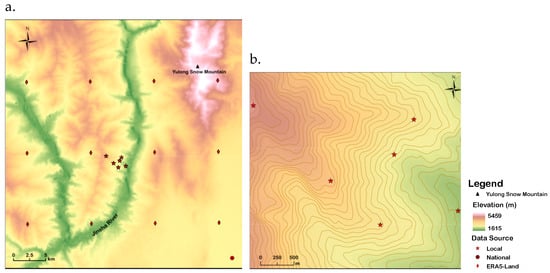
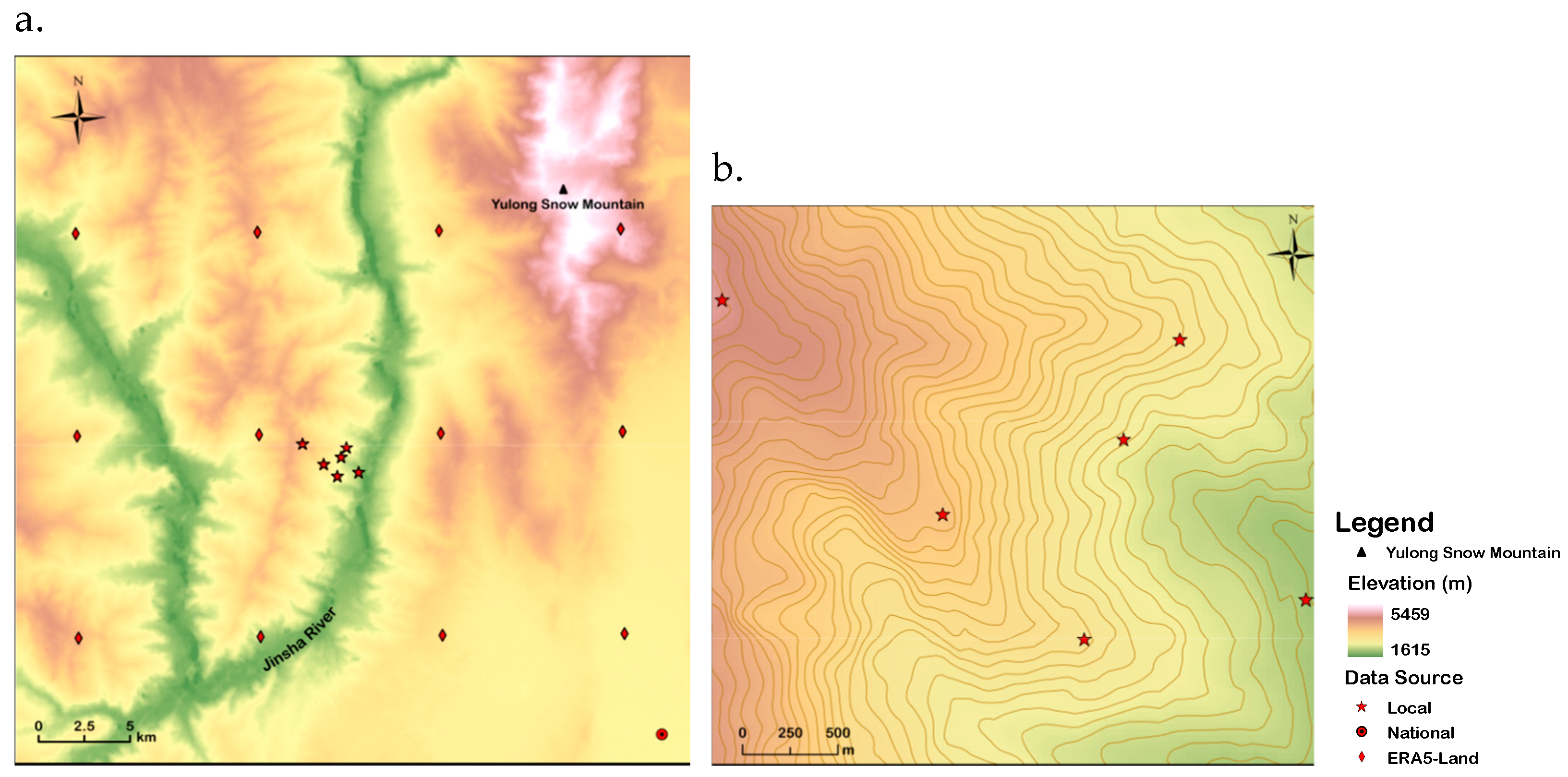
A near-surface wind sensor network of six 6 m meteorological stations was deployed in the study area (Figure 1b), recording air temperature, relative humidity, wind speed and direction, atmospheric pressure, and rainfall at 10-min intervals.

Figure 1. Spatial distribution of the three initial wind sources: (a) the entire study area; and (b) local meteorological stations.

The meteorological station layout was designed to measure airflow disturbances induced by thermal differences and to capture terrain-related airflow variations. S1 is located at the Jinsha River valley floor and represents a key node where downslope mountain winds converge at night and upslope valley winds initiate during the daytime. S2 is situated on the lower part of the northern slope and lies within a valley wind acceleration zone. S3 is positioned along the mid-slope ridge of the northern slope and serves as a primary pathway for downslope mountain winds. S4 is located on the upper southern slope and represents the core area of upslope valley-wind development. S5 is situated near the summit of the southern slope and acts as a transition zone where local circulations interact with the free atmosphere. S6 is located at the main mountain peak and is strongly influenced by the large-scale background wind.

It is worth noting that the vegetation type and height surrounding different stations within the study area vary, and vegetation height may exert a certain influence on meteorological observations. S1 is located beneath a high-voltage power line firebreak, with surrounding vegetation dominated by dense grassland of approximately 70 cm in height. S2 is situated within a Pinus yunnanensis forest. S3 is located in a small opening near the edge of the surrounding canopy, with no trees within a 5 m radius. S4 is surrounded by Pinus yunnanensis and Quercus species, resulting in partial canopy shading. S5 is located near the upper slope, where Rhododendron shrubs and young Pinus yunnanensis trees of approximately 1–3 m height are present. S6 is situated in a burned area, with sparse surrounding vegetation.

Accordingly, the locally observed wind speed and temperature at S2 and S4 may be jointly influenced by vegetation drag, enhanced turbulence, and radiative shielding effects. Although S1 and S5 lack tall trees, the presence of dense grasses and shrubs 1–3 m in height can still increase surface roughness. S3 is affected by canopy-edge effects, whereas S6-with the most open underlying surface-yields observations closer to typical near-surface boundary layer conditions.

2.2. Model and Datasets

WindNinja is a diagnostic wind-field model based on simplified physical equations that simulates terrain-induced wind flow adjustments. The model generates a spatial wind field for a given time rather than predicting future wind conditions. Inputs include terrain elevation, vegetation information, and initial wind speed and direction. WindNinja provides three wind input modes—Domain Average Wind, Point Initialization, and Weather Model—which correspond to initialization using spatially uniform wind conditions, meteorological station observations, and mesoscale numerical weather prediction data, respectively. In this study, the Point Initialization mode was used, and the version number of WindNinja employed is 3.9.0.

Three representative datasets were selected as initialization inputs for the WindNinja model: observations from local meteorological stations (Local), observations from a national meteorological station (National), and the ERA5-Land reanalysis dataset. The Local dataset was obtained from the six meteorological stations deployed within the study area. For the National dataset, the nearest Lijiang National Meteorological Station (station ID: 56651) was selected. The ERA5_Land dataset was extracted for all grid points falling within the study area, based on its spatial resolution of 0.1° × 0.1° (Figure 1a). The study period covered the entire high forest–grassland fire risk season in Yunnan Province, from 1 March to 31 May. Detailed information is provided in Table 1.

Table 1. Basic information and characteristics of the Local, National, and ERA5-Land data sources.

Initial Wind Sources	Type	Spatial Resolution	Temporal Resolution	Original Wind Height	Factors	Usage in This Study
Local	observation	station-based	10 min	6 m above the forest floor	wind speed, wind direction, temperature, etc.	local observational scale
National	observation	station-based	1 h	10 m above ground	wind speed, wind direction, temperature, etc.	operational meteorological observational scale
ERA5-Land	reanalysis data	0.1° × 0.1° grid points	1 h	10 m above ground	wind speed, wind direction, temperature, etc.	reanalysis background scale

0.1° × 0.1° denotes the grid resolution in degrees of longitude and latitude.

Given that the local meteorological stations measured wind speed at 6 m above ground within forested areas. Meanwhile, WindNinja requires wind input referenced above the surrounding vegetation; a height correction of the observed wind speed was necessary. The correction was performed based on the wind-speed conversion approach used in the FARSITE model (see Equation (1)), introducing a Wind Adjustment Factor (WAF) for calibration [14]. In this study, the observed wind speed from the local meteorological stations was approximated as midflame wind speed. According to the actual site conditions of the study area, the fuel environment was classified as Partially Sheltered Fuels, and the WAF was therefore set to 0.3. Using this factor, the observed wind speeds were converted to equivalent wind speeds at 20 ft (~6.1 m) height in open terrain, which were then used as inputs for WindNinja simulations. At the same time, the reference height for the model output wind speed was uniformly set to 20 ft to ensure consistency of wind speed height throughout the calculation process.

$$U_{20\mathrm{ft}}\approx {\displaystyle \frac{U_{\mathrm{midflame} (\approx 6\mathrm{m} \mathrm{beneath} \mathrm{the} \mathrm{canopy})}}{WAF}}$$

(1)

In addition, temporal consistency among the three datasets was required for the simulations. The National Meteorological Station data and the ERA5-Land reanalysis data are provided at hourly resolution. In contrast, the Local station observations were recorded at 10-min intervals and therefore needed to be resampled to hourly data. First, hours with missing data or calm wind conditions were identified. For each hour, if more than half of the records contained missing values or wind speeds < 0.3 m s⁻¹, that hour was marked as missing or calm and excluded. Second, the dominant wind direction and the corresponding mean wind speed for each hour were determined. Wind direction was divided into 45° sectors, and the dominant sector for each hour was identified by calculating the proportion of observations falling within each sector. A threshold of 0.5 was used for the dominant sector proportion. When the proportion of the dominant sector exceeded 0.5, the mean wind speed within that sector was calculated. When the proportion was ≤ 0.5, a temporal continuity constraint was applied, whereby the wind direction at the current time step was preferentially kept within the same sector as the previous hour. The mean wind direction and mean wind speed within the resulting dominant sector were then calculated. Through this procedure, hourly wind speed and wind direction data were derived from the Local station observations. The hourly wind data from all three sources were subsequently used as inputs to WindNinja, and the wind field corresponding to each time step was generated.

WindNinja accounts for the sheltering effect of vegetation on wind flow in a simplified manner. In the input settings, users can specify the dominant vegetation type (grass, brush, or trees) or provide a landscape file containing gridded vegetation and elevation information. Vegetation is used to define surface roughness in the model, which influences the vertical wind profile. As the study area is dominated by trees, this vegetation type was selected as the surface parameter.

WindNinja provides two solvers: (1) conservation of mass and (2) conservation of mass and momentum. The mass conservation solver runs faster but may produce lower accuracy under certain conditions. In contrast, the mass and momentum conservation solver generally provides higher accuracy but requires longer computation time and has more limited applicability. Since the latter currently does not support point initialization, the mass conservation solver was adopted in this study.

The simulation domain size and the horizontal grid resolution also need to be considered. In this study, the computational domain of WindNinja was constructed using ASTER GDEM digital elevation data with a spatial resolution of 30 m. To balance computational cost and research objectives, the output wind field was configured with a horizontal grid spacing of 100 m.

2.3. Construction of Forcing Indices

In complex mountainous environments, near-surface wind flow is typically governed by multiple interacting physical processes, including large-scale background winds, terrain-induced dynamical effects, and local circulations generated by thermally driven differential heating. The dominant physical mechanisms controlling local wind field structures can vary considerably over time, and such variability constitutes an important factor limiting the simulation accuracy.

Previous studies have indicated that WindNinja exhibits limitations under strong wind conditions. Moreover, because the model does not explicitly account for thermally driven processes, its simulation results may have limited reliability when large-scale background winds are strong or when local thermal forcing is pronounced.

To better interpret model performance under varying conditions, this study examines the relative influence of dynamical and thermal forcing. Two dimensionless indices were therefore constructed using wind speed and air temperature from the initial input data to represent the statistical intensity of these forcing mechanisms. By defining two dimensionless indices, the dominant weather background condition controlling near-surface wind fields during the study period can be quantitatively identified. This index-based framework provides a basis for analyzing systematic simulation errors in WindNinja.

2.3.1. Thermal Forcing Intensity (TFI) Index

The Thermal Forcing Intensity (TFI) index describes the relative strength of thermally driven processes over short timescales, specifically reflecting the potential for thermal circulations induced by hourly heating or cooling. The hourly air temperature change rate was first calculated for each of the three initial input datasets over the study period. These hourly temperature change rates were then mapped to their relative positions within the long-term distribution (here represented by the 90th percentile level, balancing sample size and effectively identifying anomalously strong weather-forcing scenarios) to derive a dimensionless forcing index. The calculation is expressed as follows:

$$∆T\left(t\right)=T\left(t\right)-T\left(t-1\right)$$

(2)

$$\mathrm{T}\mathrm{F}\mathrm{I}\left(t\right)={\displaystyle \frac{\mathsf{\Delta }\mathrm{T}\left(t\right)-{\Delta T}_{med}}{{\Delta T}_{P90}-{\Delta T}_{med}}}$$

(3)

Here, ${\Delta T}_{med}$ represents the median $\Delta T$ over the entire study period, and ${\Delta T}_{P90}$ denotes the 90th percentile of $\Delta T$. A TFI ≥ 1 or TFI ≤ −1 indicates strong thermal forcing.

2.3.2. Wind Forcing Intensity (WFI) Index

The Wind Forcing Intensity (WFI) index quantifies the spatial uniformity of near-surface wind fields. A higher WFI indicates greater regional consistency in wind speed and direction. When combined with the Thermal Forcing Intensity (TFI) index, conditions characterized by high WFI and low TFI can be identified as strong-wind scenarios dominated by large-scale background flow, in which synoptic forcing exerts a strong constraint on local wind-field variability. The calculation formula is as follows:

$$WFI(t)={\displaystyle \frac{ws\left(t\right)-w{s}_{med}}{w{s}_{P90}-w{s}_{med}}}$$

(4)

Here, ws_med represents the median wind speed over the entire study period, and ws_P90 denotes the 90th percentile of wind speed. A WFI ≥ 1 indicates a relatively strong wind forcing.

2.4. Scenario Classification

Based on the Thermal Forcing Intensity (TFI) and the Wind Forcing Intensity (WFI) indices, the weather-forcing scenarios throughout the study period were systematically stratified. Hourly conditions were classified into four scenarios, representing different combinations of dynamic constraints and thermal forcing:

• High_TFI + High_WFI (Strong wind under high thermal forcing): TFI ≥ 1 or TFI ≤ −1, and WFI ≥ 1;
• High_WFI (Strong wind under non-high thermal forcing): −1 < TFI < 1, and WFI ≥ 1;
• High_TFI (General weather under high thermal forcing): TFI ≥ 1 or TFI ≤ −1, and WFI < 1;
• General (General weather under non-high thermal forcing): −1 < TFI < 1, and WFI < 1.

It should be noted that this classification is not intended to strictly separate the dynamical sources of wind flow in a physical sense, but rather to identify, for different time periods, the dominant weather background condition controlling the structure of near-surface wind fields.

2.5. Evaluation Metrics and Diagnostic Strategy

The differences among the initial wind sources were diagnosed. There were inherent differences in the wind speed measurement heights provided by different datasets: the National and ERA5-Land datasets directly provide wind speeds at a height of 10 m. Meanwhile, the preprocessed Local datasets provide wind speeds at a height of 20 ft (~6.1 m), which need to be standardized before comparison. To unify the comparison baseline, the logarithmic wind profile formula [15] was applied to convert the corrected 20 ft wind speeds to 10 m height:

$$U(z)={\displaystyle \frac{u_{\ast }}{k}}\ln \left({\displaystyle \frac{z}{z_0}}\right)$$

(5)

where U(z) is the wind speed at height z, u_* is the friction velocity, k is the von Kármán constant, and z₀ is the surface roughness length.

By applying this relationship to two different heights (10 m and 6.1 m) and eliminating the unknown friction velocity u_*, the wind speed conversion formula can be derived as:

$$U_{10m}=U_{20ft}·{\displaystyle \frac{\mathit{ln}\left(\raisebox{1ex}{$10$}\!\left/ \!\raisebox{-1ex}{$z_0$}\right.\right)}{\mathit{ln}\left(\raisebox{1ex}{$6.1$}\!\left/ \!\raisebox{-1ex}{$z_0$}\right.\right)}}$$

(6)

where U_10m and U_20ft are wind speeds at 10 m and 6.1 m heights, respectively. To maintain consistency with the internal parameters of WindNinja [16], the surface roughness length z₀ was set to 1.0 m, corresponding to a vegetation type of trees, ensuring the rationality and consistency of the wind speed conversion process. Notably, the logarithmic wind profile was used only for the initial comparison and preprocessing of input data and was not involved in the subsequent wind field simulations.

After unifying the height, hourly temperature, and 10 m wind speed from the three datasets, they were averaged to obtain daily mean values, allowing a systematic comparison of the statistical differences among the datasets at the initial input stage.

Based on each dataset, the Thermal Forcing Intensity (TFI) and Wind Forcing Intensity (WFI) indices were calculated to analyze the distribution characteristics of the three initial wind sources over the entire study period. Combined with the classification of weather-forcing scenarios based on TFI and WFI, the number of samples from each initial wind source under different weather-forcing scenarios was tallied, allowing an assessment of the potential biases of each dataset in representing the dominant forcing controlling wind flow.

The hourly simulated wind fields from the three datasets were interpolated to the locations of the six local meteorological stations using bilinear interpolation and then compared with the observed values. Simulation accuracy was evaluated using Mean Bias Error (MBE), Root Mean-Square Error (RMSE), and coefficient of determination (R²), following the approach of Wilks [17]:

$$MBE={\displaystyle \frac{1}{n}}{\displaystyle \sum _{k=1}^n}\left(S_k-O_k\right)$$

(7)

$$RMSE=\sqrt{{\displaystyle \frac{1}{n}}{\displaystyle \sum _{k=1}^n}{\left(S_k-O_k\right)}^2}$$

(8)

where S_k and O_k represent the simulated and observed values, respectively.

In addition, based on the MBE of wind direction, the occurrence proportions of simulated wind direction differences within |Δθ| ≤ 11.25°, 22.5°, and 45° were calculated for the three datasets, with the two-sample Kolmogorov–Smirnov (K-S) test used to confirm the statistical significance of their distributional differences. Finally, by integrating the evaluation results with the defined weather-forcing scenarios, the dependence of model errors on weather background conditions was systematically analyzed.

3. Results

3.1. Diagnosis of Differences Among Initial Wind Sources

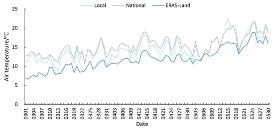
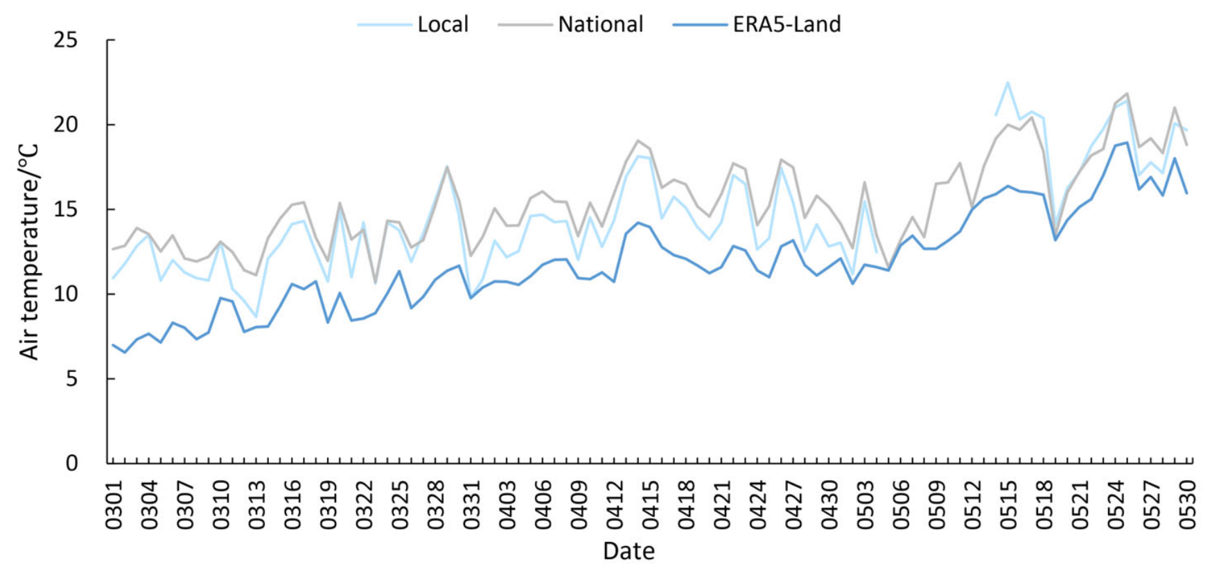
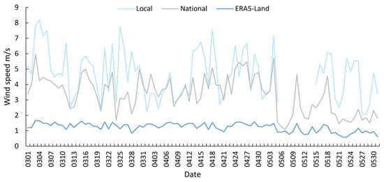
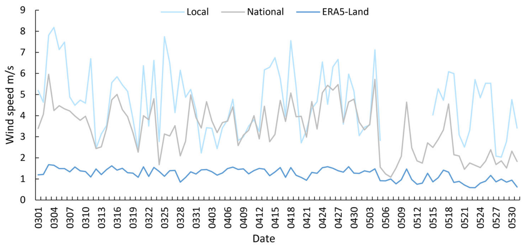
The daily mean temperature and wind speed characteristics derived from the three initial wind sources (Local, National, and ERA5-Land) were compared (Figure 2 and Figure 3). It should be noted that while the wind speeds were uniformly standardized to a 10-m reference height, the temperature data retained their original observed values without elevation normalization. The results indicate that, despite differences in their native observation heights, the three datasets exhibit highly consistent temperature trends during the study period (March to May), all characterized by a gradual warming.

Figure 2. Comparison of daily mean air temperature among the Local, National, and ERA5-Land datasets.

Figure 3. Comparison of daily mean initial wind speed among the Local, National, and ERA5-Land datasets.

Regarding daily mean wind speed, the datasets share a consistent temporal pattern but differ significantly in magnitude, following a clear ranking of Local > National > ERA5-Land. In terms of temporal variability, ERA5-Land displays the smoothest temporal evolution, with its wind-speed extremes substantially damped. In contrast, the Local data exhibits the largest amplitude of variability, capturing more intense inter-daily fluctuations. This is largely attributable to the high native temporal resolution (10-min intervals) of the Local data, which prevents the smoothing of sub-daily extremes during the aggregation into daily means.

These differences indicate that the three wind sources represent different levels of atmospheric variability, which may propagate into the WindNinja simulations and lead to distinct wind-field reconstruction results.

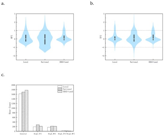
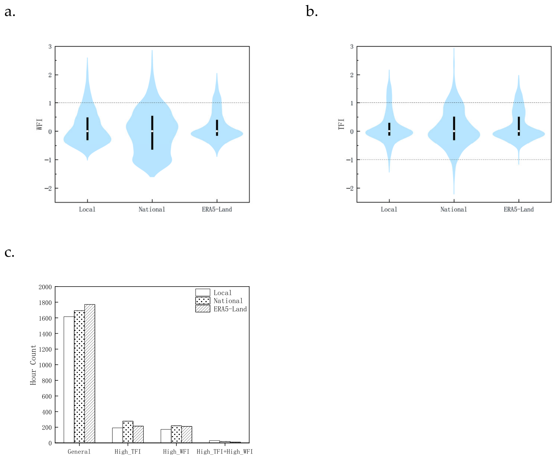
The distributions of the WFI and TFI indices derived from the three wind sources show clear structural differences (Figure 4). The WFI distribution from the National data shows the widest spread, with pronounced extensions in both the upper and lower tails, indicating stronger variability in wind-forcing conditions. In contrast, ERA5-Land produces the most concentrated distribution, with most WFI values clustered around 0, reflecting the smoothing characteristics of reanalysis data.

Figure 4. Distribution characteristics of the WFI and TFI for the three initial wind sources during the study period: (a) distribution of the WFI index; (b) distribution of the TFI index; and (c) hour counts of the four weather-forcing scenarios for each initial wind source.

Compared with WFI, the TFI distributions are generally wider for all datasets, suggesting that thermal forcing variability is more pronounced during the study period.

These differences indicate that the classification of weather-forcing scenarios is itself sensitive to the choice of the initial wind source. This sensitivity should be considered when interpreting the response of WindNinja simulation accuracy under different weather-forcing scenarios.

3.2. Comparison of WindNinja Simulation Accuracy Under Three Initial Wind Sources

The three initial wind sources exhibit systematic differences in both the direction and magnitude of wind-speed bias within the simulations (Table 2). When Local data were used to initialize WindNinja, the simulated wind speeds were generally overestimated, with the MBE at the stations ranging from 0.56 to 1.61 m s⁻¹. In contrast, simulations driven by the ERA5-Land data produced overall lower wind speeds, yielding negative MBE values across all stations. This underestimation had already been identified in the initial comparison of wind-source datasets and became further pronounced in the simulations.

Table 2. Comparison of wind speed errors between interpolated WindNinja simulations driven by three initial wind sources and Local observations (m s⁻¹).

		Average-Observed	Average-Simulated	MBE	RMSE	R2
S1	Local	1.74	2.47	0.89	2.76	0.0983
	National		2.61	0.94	3.08	0.0009
	ERA5-Land		0.88	−0.86	2.63	0.1743
S2	Local	1.56	2.61	1.17	2.38	0.2151
	National		2.22	0.70	2.49	0.0185
	ERA5-Land		1.07	−0.50	2.38	0.0168
S3	Local	3.21	4.41	1.61	3.50	0.2151
	National		3.45	0.38	3.42	0.0233
	ERA5-Land		0.87	−2.26	3.56	0.1197
S4	Local	4.13	4.41	0.56	2.95	0.3587
	National		3.79	−0.27	3.83	0.0198
	ERA5-Land		1.06	−3.08	4.50	0.0719
S5	Local	4.83	4.42	−0.07	3.66	0.2911
	National		5.02	0.35	4.43	0.1033
	ERA5-Land		1.04	−3.79	5.77	0.0139
S6	Local	4.06	4.75	1.02	3.99	0.1593
	National		5.94	2.18	5.94	0.0003
	ERA5-Land		1.12	−2.94	4.33	0.0060

It is noteworthy that the coefficient of determination (R²) between the simulated results and observations ranges from 0.0003 to 0.3587, with a median value of 0.0815, indicating an overall poor goodness-of-fit. Specifically, when simulations are driven by Local observation datasets, the R² values at S4 and S5 are relatively higher, reaching 0.3587 and 0.2911, respectively. In contrast, simulations driven by National and ERA5-Land datasets generally yield R² values below 0.1, with many cases approaching zero. These results suggest that multi-site local observations can significantly improve the model’s ability to capture wind speed variation trends in complex terrain. However, even under optimal input conditions, the proportion of variance explained by the model remains limited in such highly complex topographic settings. This highlights the current limitation of the model in reproducing microscale wind fluctuations.

A further comparison of the simulation error characteristics at different observation stations shows that simulation accuracy varies markedly with terrain positions.

In valleys (S1 and S2), simulations driven by the ERA5-Land data produced smaller wind speed errors, suggesting that smoother large-scale wind forcing can better represent mean flow conditions in open low-elevation areas.

In contrast, at ridge stations (S3, S4, and S5), ERA5-Land simulations show the largest underestimation of wind speed, whereas simulations driven by National observations perform relatively better. This suggests that coarse reanalysis winds may fail to represent terrain-induced acceleration along ridges.

At the hilltop station (S6), all simulations show larger errors compared with other stations, indicating that wind fields in exposed terrain positions are more difficult for WindNinja to reconstruct accurately.

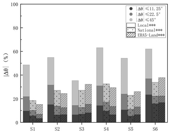
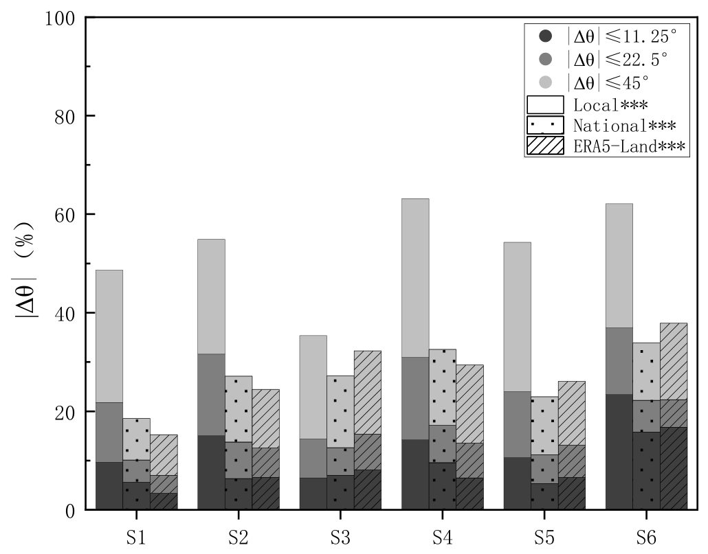
Wind direction simulations also show clear differences among the three wind sources (Figure 5), with statistically significant pairwise differences (p < 0.001). Simulations driven by Local observations produce a higher proportion of small angular errors at most stations, indicating better directional consistency with observations.

Figure 5. Cumulative distribution of angular differences between interpolated simulated and observed wind directions for the three initial wind sources. *** Indicates statistically significant differences among all pairwise comparisons (Two-sample Kolmogorov–Smirnov test, Bonferroni-corrected p < 0.001).

Among all stations, the hilltop station (S6) shows the highest proportion of small angular errors. The more exposed terrain setting likely reduces terrain blocking, allowing airflow direction to remain more consistent and enabling WindNinja to better reproduce local wind direction. Similar patterns have been reported in previous studies of wind fields in complex terrain [17].

3.3. Response of WindNinja Simulation Accuracy to Different Weather-Forcing Scenarios

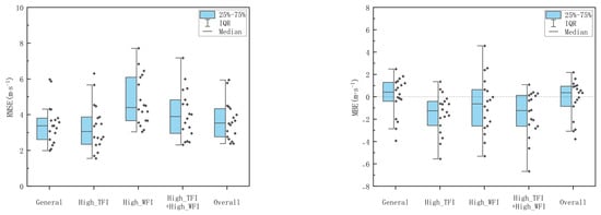
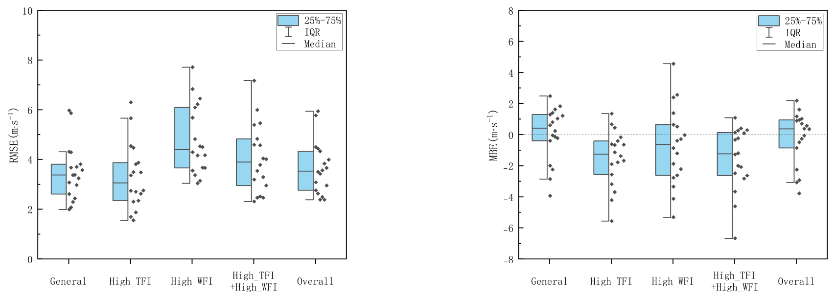
Based on the WFI and TFI indices, the study period was classified into four weather-forcing scenarios: General, High_TFI, High_WFI, and High_TFI + High_WFI. Wind-speed simulation errors show clear structural differences under these forcing conditions (Figure 6).

Figure 6. Comparison of WindNinja wind speed simulation errors under different weather-forcing scenarios.

Under the General scenario, wind speed errors remain relatively moderate and stable. When thermal forcing becomes strong (High_TFI scenario), the overall error magnitude does not increase substantially, but a noticeable negative bias appears in the simulations. This suggests that strong thermal forcing tends to introduce systematic underestimation of wind speed in WindNinja simulations.

In contrast, strong wind forcing (High_WFI scenario) significantly amplifies both the magnitude and dispersion of simulation errors. The wider range of wind-speed errors indicates lower model reliability under strong wind-forcing conditions.

Under compound forcing conditions (High_TFI + High_WFI scenario), the dispersion of wind speed errors increases further, and the negative bias becomes more pronounced. This indicates that the interaction between dynamic and thermal forcing can complicate the wind field structure and lead to more unstable model performance.

Overall, the magnitude and variability of wind-speed simulation errors are primarily controlled by wind forcing intensity. In contrast, strong thermal forcing tends to cause a systematic and stable decline in simulation accuracy.

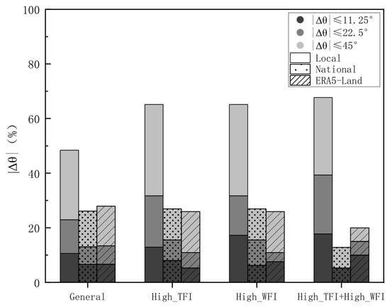
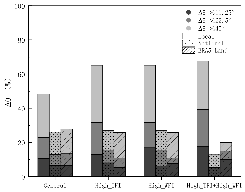
Wind direction simulations also respond differently to the various forcing scenarios (Figure 7). For simulations driven by Local data, the proportion of small angular errors gradually increases as forcing intensity strengthens. In contrast, simulations driven by National data and ERA5-Land data show a decreasing proportion of small angular errors under compound forcing conditions.

Figure 7. Comparison of wind direction simulation errors for the three data sources under different weather-forcing scenarios.

These results suggest that the interaction between dynamic and thermal forcing may amplify directional uncertainties in simulations driven by coarse wind sources. Meanwhile, high-resolution local observations provide more stable directional constraints for WindNinja.

4. Discussion

4.1. Input Sensitivity of WindNinja to Initial Wind Sources

The results indicate that simulations produced by WindNinja are significantly influenced by the initial input data, a characteristic closely related to its diagnostic model framework. Rather than solving the atmospheric momentum equations directly, WindNinja dynamically adjusts the wind velocity vectors based on the principle of mass conservation under given initial conditions [18]. Consequently, the initial wind sources not only determine the magnitude of the simulated wind speed but also largely constrain the degree of adjustment that the model can perform.

Local data can provide more detailed information on local wind conditions, and simulations driven by these data generally show better overall performance. However, the simulated wind speeds tend to be systematically overestimated. This bias may partly arise from systematic errors introduced during the wind speed conversion process. In complex terrain, the use of a uniform WAF value of 0.3 represents an idealized simplification. Although this parameter may be appropriate for partially sheltered forested environments, higher WAF values should be applied for stations such as S1, S3, S5, and S6, where vegetation shielding is relatively weak [19]. Applying a relatively low WAF to these stations may artificially increase the 20-ft input wind speed, which in turn propagates through the model dynamics and leads to an overall overestimation of simulated wind speeds across the study domain. Future studies should carefully address the treatment of initial input data in order to further disentangle errors arising from input preprocessing and those inherent to the modeling framework.

In contrast, the simulated wind speed driven by ERA5-Land data is generally low. This dataset was diagnosed as low wind speed during the initial wind-source comparison, and even after complex-terrain adjustments in the model, it still shows negative bias. This result indicates that, as a diagnostic model, WindNinja tends to inherit biases present in the initial input data, and its terrain-adjustment process cannot effectively correct systematic biases already contained in the initial wind sources. It also suggests that although complex terrain effects can substantially reshape the spatial distribution of the wind field, the magnitude of simulated wind speeds remains largely constrained by the initial input data. Therefore, increasing the resolution of the initial wind source does not necessarily lead to improved accuracy in wind speed simulations [13,20].

4.2. Error Structures of WindNinja Across Different Terrain Positions

The simulation accuracy of WindNinja exhibits pronounced spatial heterogeneity, with distinct error structures observed across different terrain positions. Specifically, stations located in valleys or low-lying areas experience near-surface wind fields that are strongly influenced by terrain channeling and sheltering effects, resulting in a relatively limited range of wind speed variability. Consequently, wind speed simulation errors at these stations are generally smaller, suggesting that the model shows relatively stable performance in reproducing wind speed under strong terrain constraints. However, the local airflow direction at these sites can easily shift with terrain morphology, leading to strong spatial variability in wind direction and, therefore, relatively larger wind direction simulation errors. In contrast, stations situated on ridges or hilltops, which are relatively exposed locations, experience less terrain obstruction to the incoming flow. As a result, the wind direction structure tends to exhibit greater temporal consistency. At these locations, WindNinja performs relatively well in reproducing wind direction changes, resulting in smaller angular errors in simulated wind direction. However, because wind speed at these exposed sites is more strongly influenced by both incoming flow variability and terrain-induced acceleration effects, the corresponding wind speed simulation errors also tend to increase.

These results indicate that the error structure of WindNinja varies across different terrain positions. In sheltered terrain, simulation errors are mainly reflected in wind direction, whereas in exposed terrain, errors are more prominently manifested in wind speed magnitude. This difference in error structure has important implications for the interpretation and application of WindNinja results.

This result further indicates that terrain complexity significantly affects the simulation accuracy of WindNinja. This influence does not arise solely from the degree of terrain relief itself, but is also reflected in the fact that, under complex terrain conditions, the initial input data experience a substantially greater number of dynamic adjustment pathways during the downscaling process [21,22]. In complex terrain, once the initial input data enter the model domain, they are simultaneously influenced by multiple dynamical processes, including terrain channeling, sheltering, terrain-induced acceleration, and channel effects. These combined processes make the simulated wind speed and direction highly sensitive to the quality of terrain information and relative terrain position [23]. Because the construction of the wind field in WindNinja relies primarily on terrain information and initial input data, and lacks representation of higher-order dynamical processes, terrain-based adjustments alone are insufficient to fully reproduce the fine-scale structural characteristics of wind fields in complex terrain. As a result, the model’s ability to accurately simulate wind fields becomes limited under conditions of high terrain complexity.

4.3. Response of WindNinja Under Different Weather-Forcing Scenarios

By introducing the WFI and TFI indices to classify the weather background conditions into different scenarios, the study period was divided into four categories: general weather and strong-wind conditions under both high-thermal-forcing and non–high-thermal-forcing environments. Based on this classification, the study further investigated how the simulation accuracy of WindNinja responds to different weather-forcing scenarios.

The results show that dynamic constraints are the dominant factor influencing the simulation accuracy of WindNinja, with error levels responding most strongly to variations in wind forcing intensity. Under non–high-thermal-forcing conditions, as the weather-forcing scenarios shift from general weather to strong wind conditions, wind speed errors rapidly increase. The simplified dynamic framework of WindNinja struggles to accurately capture the complex nonlinear interactions among terrain-induced acceleration, flow diversion, and other processes under high wind speeds. Previous studies have indicated that in complex terrain, wind speed exhibits a nonlinear relationship with incoming flow intensity and is strongly influenced by terrain-guidance effects, which simple diagnostic models cannot fully reproduce [24]. Therefore, in weather scenarios dominated by strong-wind conditions, the growth of model errors with increasing WFI is a natural consequence of the model’s dynamic assumptions.

Meanwhile, differences in the error structure under varying thermal forcing conditions indicate that the absence of thermal processes also has a significant impact on model accuracy. As thermal forcing increases, model errors do not exhibit random fluctuations; instead, they show stable and identifiable patterns in simulation accuracy, specifically manifesting as an amplification of systematic negative bias and a tendency toward more concentrated error distributions. This indicates that WindNinja’s mass-conserving diagnostic framework responds consistently to changes in the thermal forcing. The results show that under high thermal-forcing conditions, wind speed errors remain significantly higher than in non-thermal-forcing scenarios, even when wind-forcing intensity is not strong. When thermal forcing intensifies—such as slope winds or valley breezes triggered by strong insolation, or pronounced thermal buoyancy—local wind direction and shear structures can change markedly, processes that are not directly represented in WindNinja’s physical framework. In addition, under nocturnal stable boundary layer conditions, thermal processes can affect near-surface wind fields through inversion structures [25,26]. Such thermally–dynamically coupled phenomena are difficult to reconstruct using a single background wind field through diagnostic adjustments alone [12,27].

4.4. Impacts of WindNinja Simulated Wind Fields on Fire Spread and Associated Uncertainties

Previous studies have shown that terrain-driven local wind fields are a dominant factor controlling potential fire behavior [28]. In this study, WindNinja simulations reveal that under the strongly heterogeneous topographic conditions of the study area, near-surface wind fields exhibit pronounced spatial variability, manifested as slope acceleration zones, valley channeling effects, and ridgeline wind direction shear. These microscale features exert direct control on fire behavior evolution: slope wind acceleration can strongly promote upslope fire spread, channeling effects in valleys facilitate fireline convergence and intensification, and strong wind-direction shear near ridges can readily trigger abrupt transitions in fire behavior [29,30,31]. The high-resolution wind fields provided by WindNinja effectively capture these terrain-modulated effects, offering critical spatially explicit information for identifying preferential fire spread pathways and high-risk areas.

However, the practical application of such fine-scale spatial patterns is not without cost, with the primary challenge lying in the model’s high sensitivity to initial input data. In this study, a fixed wind adjustment factor (WAF) was used to convert wind speeds from local meteorological stations to the model reference height. In reality, vegetation structure varies across stations in the study area, leading to corresponding differences in vertical wind profiles [32]. Although the use of a uniform WAF ensures data standardization, it inevitably introduces systematic bias into the input wind field. This distortion in the initial wind field can directly affect fire spread simulations, leading to significant uncertainty in predicted fire propagation direction and rate.

In addition, the relatively low coefficient of determination (R²) between simulated and observed data further indicates that WindNinja is unable to fully reproduce short-term fluctuations in near-surface wind fields under complex terrain conditions. This discrepancy may arise, on the one hand, from the model’s limited ability to represent turbulent structures [21], and on the other hand, from the limited spatial representativeness of point observations, which cannot fully represent grid-scale mean wind fields, thereby introducing inconsistencies in model–observation comparisons. Therefore, WindNinja is more suitable for capturing spatial patterns and relative variations in wind fields, while its accuracy in absolute wind speed remains limited. In wildfire risk assessment applications, this limitation must be carefully acknowledged, as it may introduce uncertainty in predicting localized fire behavior transitions or extreme events such as spot fires.

5. Conclusions

This study employed three types of initial wind sources (Local, National, and ERA5-Land) to drive the WindNinja model and conducted high-resolution near-surface wind field simulations in a complex terrain. The accuracy of the model in simulating wind speed and wind direction was systematically evaluated. The results show that WindNinja exhibits strong input sensitivity, with its simulation accuracy jointly controlled by initial wind sources, terrain conditions, and weather background.

The influence of the initial wind source on simulation results shows clear directional and predictable patterns. Terrain position further regulates the error structure of the simulations, which is largely determined by the relative effects of terrain shielding and local wind acceleration. Weather-forcing conditions also play a significant role in controlling simulation accuracy. Wind forcing intensity is identified as the primary factor governing the magnitude and dispersion of simulation errors, whereas strong thermal forcing tends to produce a systematic decline in simulation accuracy and stability. The scenario-based analytical framework established using the Wind Forcing Intensity (WFI) and Thermal Forcing Intensity (TFI) indices provides an effective approach for identifying the applicability of WindNinja and diagnosing potential error sources under different weather background conditions.

Based on these findings, several directions for future improvement are suggested. First, the quality of initial wind sources could be enhanced through multi-source data fusion or scenario-based selection of optimal wind sources. Second, terrain-related parameters such as terrain shielding and local acceleration could be incorporated as auxiliary indicators for post-simulation bias correction. Third, thermal influences may be indirectly considered by introducing indicators representing boundary-layer stability or surface heating intensity (e.g., the air temperature change rate) into scenario classification or post-processing correction, thereby improving simulation accuracy under thermally dominated conditions.

References

- Sharples, J.J. An overview of mountain meteorological effects relevant to fire behaviour and bushfire risk. Int. J. Wildland Fire 2009, 18, 737–754. [Google Scholar] [CrossRef] [Scilit]
- Wani, A.H.; Varma, R.K.; Ahuja, A.K. Experimental investigation of wind flow characteristics over hills and escarpments: A review. Wind Struct. 2021, 32, 393–403. [Google Scholar] [CrossRef]
- Butler, B.W.; Wagenbrenner, N.S.; Forthofer, J.M.; Lamb, B.K.; Shannon, K.S.; Finn, D.; Eckman, R.M.; Clawson, K.; Bradshaw, L.; Sopko, P.; et al. High-resolution observations of the near-surface wind field over an isolated mountain and in a steep river canyon. Atmos. Chem. Phys. 2015, 15, 3785–3801. [Google Scholar] [CrossRef] [Scilit]
- Butler, B.; Quarles, S.; Standohar-Alfano, C.; Morrison, M.; Jimenez, D.; Sopko, P.; Wold, C.; Bradshaw, L.; Atwood, L.; Landon, J.; et al. Exploring fire response to high wind speeds: Fire rate of spread, energy release and flame residence time from fires burned in pine needle beds under winds up to 27 m s−1. Int. J. Wildland Fire 2020, 29, 81–92. [Google Scholar] [CrossRef] [Scilit]
- Liu, N.; Lei, J.; Gao, W.; Chen, H.; Xie, X. Combustion dynamics of large-scale wildfires. Proc. Combust. Inst. 2021, 38, 157–198. [Google Scholar] [CrossRef] [Scilit]
- Yan, W.; Liu, N.; Zhu, H.; Chen, H.; Xie, X.; Gao, W.; Du, Z. Firebrand burning under wind: An experimental study. Int. J. Wildland Fire 2024, 33, WF23151. [Google Scholar] [CrossRef] [Scilit]
- Wang, W.; Chen, F. Wind field modeling over hilly terrain: Methods, challenges, limitations, and future directions. Appl. Sci. 2025, 15, 10186. [Google Scholar] [CrossRef] [Scilit]
- Forthofer, J.M.; Butler, B.W.; McHugh, C.W.; Finney, M.A.; Bradshaw, L.S.; Stratton, R.D.; Shannon, K.S.; Wagenbrenner, N.S. A comparison of three approaches for simulating fine-scale surface winds in support of wildland fire management. Part II: Effect of simulated winds on fire growth simulations. Int. J. Wildland Fire 2014, 23, 982–994. [Google Scholar] [CrossRef] [Scilit]
- Wang, A.; Wang, C.; Gao, G.; Wu, N.; Su, H. Quantitative assessment of firefighting danger based on numerical simulation of forest fire spread in canyon wind fields. PLoS ONE 2025, 20, e0328733. [Google Scholar] [CrossRef] [Scilit] [PubMed]
- Poudel, R.C.; Tinnesand, H.; Baring-Gould, I.E. An evaluation of advanced tools for distributed wind turbine performance estimation. J. Phys. Conf. Ser. 2020, 1452, 012017. [Google Scholar] [CrossRef] [Scilit]
- Novikarany, R.; Briliano, B. Evaluasi model prediksi angin permukaan pada wilayah rawan kebakaran hutan: Kasus WindNinja di Kalimantan Selatan. J. Sains Teknol. Modif. Cuaca 2024, 25, 71–80. Available online: https://ejournal.brin.go.id/JSTMC/article/view/5758 (accessed on 10 May 2026).
- Seto, D.; Jones, C.; Siuta, D.; Wagenbrenner, N.; Thompson, C.; Quinn, N. Evaluation of HRRR wind speed forecast and WindNinja downscaling accuracy during Santa Ana wind events in Southern California. Weather Forecast. 2025, 40, 525–541. [Google Scholar] [CrossRef] [Scilit]
- Wagenbrenner, N.S.; Forthofer, J.M.; Lamb, B.K.; Shannon, K.S.; Butler, B.W. Downscaling surface wind predictions from numerical weather prediction models in complex terrain with WindNinja. Atmos. Chem. Phys. 2016, 16, 5229–5241. [Google Scholar] [CrossRef] [Scilit]
- Andrews, P.L. Modeling Wind Adjustment Factor and Midflame Wind Speed for Rothermel’s Surface Fire Spread Model; General Technical Report RMRS-GTR-266; U.S. Department of Agriculture, Forest Service, Rocky Mountain Research Station: Fort Collins, CO, USA, 2012; p. 39.
- Stull, R.B. Similarity theory. In An Introduction to Boundary Layer Meteorology; Atmospheric Sciences Library; Springer: Dordrecht, The Netherlands, 1988; Volume 13. [Google Scholar] [CrossRef] [Scilit]
- Quill, R.; Sharples, J.J.; Wagenbrenner, N.S.; Sidhu, L.A.; Forthofer, J.M. Modeling wind direction distributions using a diagnostic model in the context of probabilistic fire spread prediction. Front. Mech. Eng. 2019, 5, 5. [Google Scholar] [CrossRef] [Scilit]
- Wilks, D.S. Statistical Methods in the Atmospheric Sciences: An Introduction; Academic Press: San Diego, CA, USA, 1995; p. 467. [Google Scholar]
- Forthofer, J.M.; Butler, B.W.; Wagenbrenner, N.S. A comparison of three approaches for simulating fine-scale surface winds in support of wildland fire management. Part I: Model formulation and comparison against measurements. Int. J. Wildland Fire 2014, 23, 969–981. [Google Scholar] [CrossRef] [Scilit]
- Massman, W.J.; Forthofer, J.M.; Finney, M.A. An improved canopy wind model for predicting wind adjustment factors and wildland fire behavior. Can. J. For. Res. 2017, 47, 594–603. [Google Scholar] [CrossRef] [Scilit]
- Wang, W.; Shaw, W.J.; Seiple, T.E.; Rishel, J.P.; Xie, Y. An evaluation of a diagnostic wind model (CALMET). J. Appl. Meteorol. Climatol. 2008, 47, 1739–1756. [Google Scholar] [CrossRef] [Scilit]
- Wagenbrenner, N.; Atwood, L.; Forthofer, J.; Grenfell, I. Predicting terrain-induced wind turbulence for smokejumper parachute operations. Int. J. Wildland Fire 2024, 33, WF24112. [Google Scholar] [CrossRef] [Scilit]
- Buchs, M. Evaluation of WindNinja Simulations in Canyons and Complex Terrain. Master’s Thesis, San Jose State University, San Jose, CA, USA, 2025. [Google Scholar] [CrossRef] [Scilit]
- Mallare, R.A.; Shintani, T.; Yokoyama, K. Estimation of non-uniform wind fields over a meandering reservoir. J. Jpn. Soc. Civ. Eng. Ser. B1 (Hydraul. Eng.) 2022, 78, I_1039–I_1044. [Google Scholar] [CrossRef] [Scilit] [PubMed]
- Dimitrov, T.; Chervenkov, H. Preliminary results from the exploration of the WindNinja model at the local scale over Bulgaria. In Environmental Protection and Disaster Risks (EnviroRisks 2024); Dobrinkova, N., Fidanova, S., Eds.; Lecture Notes in Networks and Systems; Springer: Cham, Switzerland, 2025; Volume 883. [Google Scholar] [CrossRef] [Scilit]
- Mahrt, L. Stably Stratified Boundary Layer. In Encyclopedia of Atmospheric Sciences; Holton, J.R., Ed.; Academic Press: San Diego, CA, USA, 2003; pp. 298–305. [Google Scholar] [CrossRef] [Scilit]
- Lan, C.; Liu, H.; Li, D.; Katul, G.G.; Finn, D. Distinct turbulence structures in stably stratified boundary layers with weak and strong surface shear. J. Geophys. Res. Atmos. 2018, 123, 7839–7854. [Google Scholar] [CrossRef] [Scilit]
- Wagenbrenner, N.S.; Forthofer, J.M.; Page, W.G.; Butler, B.W. Development and evaluation of a Reynolds-averaged Navier–Stokes solver in WindNinja for operational wildland fire applications. Atmosphere 2019, 10, 672. [Google Scholar] [CrossRef] [Scilit]
- Robinson, D.; Brambilla, S.; Oliveto, J.; Brown, M.J.; Atchley, A.; Linn, R.R. The effect of terrain-influenced winds on fire spread in QUIC-Fire. Environ. Model. Softw. 2023, 167, 105727. [Google Scholar] [CrossRef] [Scilit]
- Sánchez-Monroy, X.; Mell, W.; Torres-Arenas, J.; Butler, B.W. Fire spread upslope: Numerical simulation of laboratory experiments. Fire Saf. J. 2019, 108, 102844. [Google Scholar] [CrossRef] [Scilit]
- Abouali, A.; Viegas, D.X.; Raposo, J.R. Analysis of the wind flow and fire spread dynamics over a sloped–ridgeline hill. Combust. Flame 2021, 234, 111724. [Google Scholar] [CrossRef] [Scilit]
- Hayajneh, S.M.; Alzghoul, M.I.; Naser, J. Wind and slope effects on wildland fire spread: A review of experimental, empirical, mathematical, and physics-based models. Fire 2026, 9, 100. [Google Scholar] [CrossRef] [Scilit]
- Maurer, K.D.; Hardiman, B.S.; Vogel, C.S.; Bohrer, G. Canopy-structure effects on surface roughness parameters: Observations in a Great Lakes mixed-deciduous forest. Agric. For. Meteorol. 2013, 177, 24–34. [Google Scholar] [CrossRef] [Scilit]
Disclaimer/Publisher’s Note: The statements, opinions and data contained in all publications are solely those of the individual author(s) and contributor(s) and not of MDPI and/or the editor(s). MDPI and/or the editor(s) disclaim responsibility for any injury to people or property resulting from any ideas, methods, instructions or products referred to in the content. |
© 2026 by the authors. Licensee MDPI, Basel, Switzerland. This article is an open access article distributed under the terms and conditions of the Creative Commons Attribution (CC BY) license.