


Abstract
Near-real-time wildfire monitoring is essential for situational awareness and emergency response. The Geostationary Operational Environmental Satellite (GOES) observes at 2 km every 5 min, whereas the Visible Infrared Imaging Radiometer Suite (VIIRS) observes at 375 m twice daily, leaving neither sensor able to track rapidly evolving fires in fine spatial detail. This study introduces a two-step deep learning approach that statistically infers VIIRS-like sub-pixel fire segmentation and brightness temperature (BT) from GOES imagery. The dataset comprises 257 U.S. wildfires within preselected regions of interest, pairing multi-spectral GOES imagery with VIIRS-derived references in four classes (Non-Fire, Small, Medium, and Large) defined by the number of fire pixels. Against an autoencoder-based baseline, the proposed method raises average precision from 0.105 to 0.368 and reduces the fire region BT root mean square error by 72.1% from 81.33 K to 22.69 K. Omission error rates fall from 9.41% to 1.96% for Medium fires and remain at zero for Large fires, whereas Small fires, 37% of the test set, remain at 39.91%. The false positive rate on Non-Fire images falls from 66.86% to 8.48%, near the operational GOES product’s 6.36% with lower omission (31.40% versus 40.35%). Inference completes within 5 min of observation for a monitored region.
1. Introduction
Wildfires have emerged as one of the most destructive and fast-growing natural hazards in the United States, with far-reaching impacts on communities, ecosystems, public health, and the economy. In 2023, the United States recorded 56,580 wildfires that burned 1.09 million hectares (2.7 million acres) and destroyed at least 4318 structures [1]. Active-fire response, an important part of wildfire management strategy, requires wildfire monitoring solutions that are fast, accurate, cost-effective, and spatially detailed. In operational contexts, detecting fire presence alone is insufficient. Operational systems must instead deliver georeferenced maps that accurately locate active fires and characterize their thermal signal, ideally with near-real-time latency.
Traditional wildfire monitoring systems, such as ground-based cameras, airborne sensors, and human reports, provide localized insights but suffer from information latency, high deployment costs, coverage gaps, and logistical challenges, especially when monitoring large or inaccessible areas. In contrast, satellite remote sensing offers a scalable and consistent means of observing vast landscapes. Among available satellites, polar-orbiting platforms such as Visible Infrared Imaging Radiometer Suite (VIIRS) and Moderate Resolution Imaging Spectroradiometer (MODIS) provide global coverage with spatial resolutions that are relevant to wildfire management problems (e.g., 375 m and 1 km, respectively). However, their temporal frequency is limited to just a few overpasses per day, which is often insufficient for tracking the rapid progression of wildfires. Geostationary satellites offer a compelling alternative. While they observe a fixed portion of the Earth’s surface at relatively low spatial resolution, they provide semi-continuous coverage over large regions at higher temporal resolution. For example, the Geostationary Operational Environmental Satellite-R (GOES-R) series, comprising GOES-16 through GOES-19, monitors the Americas. Although its infrared bands offer a relatively coarse spatial resolution of approximately 2 km compared to polar-orbiting sensors, the 5 min temporal frequency of GOES imagery makes it a valuable resource for near-real-time wildfire monitoring.
One of the most widely used methods is the Wildfire Automated Biomass Burning Algorithm (WF-ABBA), a dynamic contextual thresholding algorithm that has played a foundational role in operational fire detection [2,3,4]. It utilizes the 3.9 μm Middle Infrared (MIR) and 10.7 μm Thermal Infrared (TIR) bands, along with the visible band when available. It also incorporates the 12 μm band to help distinguish hot targets from opaque cloud cover. Despite its success, WF-ABBA suffers from limitations, including a high false-alarm rate due to atmospheric conditions such as solar reflectance and cloud edges, coarse spatial resolution, and an inability to resolve small or low-intensity fires [5,6]. To improve reliability, alternative thresholding-based frameworks such as the GOES Early Fire Detection (GOES-EFD) system were introduced, yet these methods remain constrained by predefined rules and sensitivity to atmospheric conditions [7]. The current operational GOES ABI Fire Detection and Characterization (FDC) product extends WF-ABBA and serves as a reference in this study [8].
To overcome the limitations of thresholding-based detection methods, recent studies explored deep learning (DL) models for automatic fire segmentation using satellite imagery. Toan et al. [9] presented one of the earliest DL studies to leverage GOES imagery for wildfire detection. This work was notable for being the first to aim toward a real-time streaming platform for wildfire monitoring based on pixel-wise classification. The authors utilized all 16 spectral bands from GOES-R, treating each multi-band image as a 3D input volume. The proposed model was a simple deep convolutional neural network (CNN) composed of 3D convolutional layers followed by fully connected layers, trained to classify each patch as fire or Non-Fire based on its center pixel label. Zhao and Ban [5] employed a temporal modeling strategy that applied Gated Recurrent Units to GOES-R time series imagery, which allowed the network to capture dynamic fire behavior over time. The input to the model was preprocessed using dedicated spectral indices, including a normalized difference between the MIR and TIR bands to enhance fire signals, and a custom smoke/cloud mask based on the 12.3 μm band (Band 15). Using VIIRS active fire points as supervisory labels, the network was trained to segment burning areas. The results showed improved early detection capability and spatial localization compared to the GOES-R operational active fire product, while also reducing false positive detection in mid-latitude regions. These developments demonstrate a growing shift toward data-driven approaches, where past snapshots are incorporated into the monitoring process. However, despite these advances, Koltunov et al. [6] and Zhao and Ban [5] relied on combining specific subsets of GOES bands using predefined equations and thresholds, which can ultimately lead to loss of valuable information. Additionally, studies including Malik et al. [10] and Toan et al. [9] were restricted to limited spatial domains, which hindered generalizability and operational scalability. Moreover, many models, such as Badhan et al. [11] and Toan et al. [9], used polar-orbiting VIIRS/MODIS data for supervision without accounting for the spatial disparities between GOES and VIIRS observations. These limitations highlight the need for a data-driven approach that exploits multi-spectral information from GOES imagery, scales to a continental domain, and explicitly accounts for spatial and temporal disparities between geostationary and polar-orbiting observations.
In a recent work [11], a DL framework was developed to infer fine-scale fire patterns from GOES-17 imagery. The model was trained using contemporaneous GOES–VIIRS observation pairs. Its objective was to generate VIIRS-scale fire maps at GOES’s high temporal frequency, enabling more accurate estimation of fire location and brightness temperature (BT). Although the potential of this approach was demonstrated, it tended to underestimate BT values compared to the VIIRS reference data. To address this critical challenge, here we propose a more general framework for near-real-time monitoring of wildfire events located across the contiguous United States (CONUS) and Hawaii. A key novelty of this work is a two-step DL pipeline, which is designed to address the underestimation of the BT values at fire locations. In this approach, segmentation first isolates fire-affected regions, and regression then estimates sub-pixel BT, outperforming the single-step approach in the prior work [11]. Since this framework prioritizes consistency with the co-registered GOES and VIIRS training pairs, generative approaches are not employed, as they risk producing spatially plausible fire structures that are not constrained by observations.
Furthermore, several other technical advancements are introduced over the previous work [11]. These include leveraging a broader set of GOES spectral bands to correct for environmental effects and improving preprocessing through parallax correction and normalization. We also examine the effects of hyperparameter choices, such as background value selection and loss function design, through a comprehensive ablation study. Finally, the near-real-time latency of the framework is assessed based on GOES-18 data availability on a public archive. These advancements address the key limitations of the earlier model and enable improved fire region BT estimation and active fire segmentation.
The remainder of the paper is organized as follows. Section 2 describes the satellite data sources and outlines the preprocessing steps for dataset construction and alignment. Section 3 details the proposed two-step segmentation-regression approach, including the DL architecture, loss functions, and evaluation metrics. Section 4 presents the training and testing results, including quantitative and visual evaluations, and discusses the impact of different loss functions and weights as well as background values through ablation studies. Section 5 assesses the near-real-time latency of the proposed pipeline. Finally, Section 6 concludes the paper with a summary of key findings and directions for future work.
2. Data Sources and Preprocessing
In this study, a wildfire dataset is developed to support training the DL model. The dataset is constructed from open-source satellite imagery and products, including low-spatial-resolution GOES imagery used as the model input and the VIIRS active fire product serving as the reference. This work advances the prior efforts of Badhan et al. [11] by improving the data quality, extending spatial and temporal coverage, incorporating additional spectral features, and correcting spatial misalignments. Fire event splits are kept disjoint across training and test sets to prevent data leakage. Data sources, region of interest (ROI), and dataset construction are described in this section.
2.1. Products and Data Sources
Two primary satellite products are used to construct the dataset, namely VIIRS I-band Active Fire Product [12] and GOES Advanced Baseline Imager (ABI) Cloud and Moisture Imagery product (ABI-CMIPC) [13]. VIIRS is onboard the Suomi-NPP, NOAA-20, and NOAA-21 satellites in polar orbits. Each satellite provides approximately two observations per day over most locations, with one ascending and one descending overpass, typically occurring during daytime and nighttime, respectively. The VIIRS I-band Active Fire Product detects fire locations using an algorithm described in the Algorithm Theoretical Basis Documents (ATBD) [14,15,16], which integrates multiple spectral bands to identify thermal anomalies. The algorithm identifies active fires through a sequence of fixed threshold and contextual tests. The algorithm uses BT values from bands I4 (3.55–3.93 μm) and I5 (10.50–12.40 μm), reflectance from I1 (0.60–0.68 μm), I2 (0.85–0.89 μm), and I3 (1.58–1.64 μm), along with geometric parameters such as solar and view zenith angles and relative azimuth, as well as moderate-resolution bands like M13 (3.97–4.13 μm) to address the I4 saturation problem and to calculate Fire Radiative Power (FRP).
The algorithm begins by classifying clouds and water bodies using BT value and reflectance thresholds from I1, I2, I3, and I5. Fixed thermal threshold tests are then applied to I4 and I5 to capture strong thermal anomalies typical of active fires, with special handling for saturated and folded I4 pixels that may otherwise produce classification errors. Pixels with anomalous MIR signals caused by such data artifacts are identified and treated separately as potential background fire pixels. Subsequently, additional exclusion tests are applied to identify and flag pixels affected by sun glint or bright surfaces (e.g., urban areas or bare soils) using geometric parameters and reflectance-based criteria. Candidate fire pixels are then selected using a dynamically adjusted I4 threshold rather than a fixed one. This threshold is derived from the median I4 BT value within a 501 × 501 sampling window centered on the pixel and is clamped to the range of 325 K to 330 K, and it is applied to daytime data only, whereas a single fixed value is used at night. For each candidate fire pixel, background conditions are subsequently characterized using a sampling window that expands from 11 × 11 to 31 × 31 pixels until at least 25% of the window pixels or at least 10 valid pixels are found. Valid pixels exclude clouds, potential background fire pixels, and non-nominal quality data, and are restricted to the same surface class (land or water) as the candidate. Contextual fire detection tests then compare the candidate’s thermal signal to this background using both absolute and relative BT differences. If insufficient valid pixels are available for background characterization, the pixel is labeled “unclassified.” Candidates that pass contextual tests are assigned a confidence level of low, nominal, or high, based on the strength of their anomaly, viewing geometry, and potential contamination. Secondary tests further identify residual low-confidence fires and screen out remaining false positives, particularly in sun glint zones and regions affected by the South Atlantic Magnetic Anomaly. The resulting detections are distributed by NASA Fire Information for Resource Management System (FIRMS) in CSV format and include fire coordinates, confidence levels, BT values from the I4 and I5 bands, and FRP. This product serves as the reference in this study. It is worth noting that, as a threshold-based, context-dependent detection product, the VIIRS active fire product carries inherent limitations, as it may miss low-intensity or obscured fires and can be affected by saturation and folding artifacts [16]. We partially mitigate these issues by excluding affected pixels from the evaluation processes as described in Section 2.2. However, the model is ultimately trained to reproduce a processed product, thereby inheriting the biases and omissions of the VIIRS data product rather than independently characterizing fire.
The second satellite product, GOES ABI-CMIPC, provides Cloud and Moisture Imagery (CMI) derived from ABI measurements across 16 spectral bands spanning the visible (0.47 μm) to infrared (13.3 μm) wavelengths. For reflective bands (1–6), the CMI product stores reflectance factors normalized by the solar zenith angle, while for emissive bands (7–16), BT values at the top of atmosphere are provided directly. Only the BT values from relevant infrared bands are used in this study. These data are provided in the NetCDF format and sourced from the GOES-East and GOES-West satellites. The GOES satellites jointly provide continuous multi-spectral coverage across the United States with a temporal resolution of 5 min. GOES-16 has operated as GOES-East throughout the study period, while GOES-18, which replaced GOES-17 in January 2023, has operated as GOES-West [17]. To ensure uninterrupted spatial and temporal coverage, data from GOES-16, GOES-17, and GOES-18 are all included, with the appropriate satellite selected based on each wildfire’s location and timestamp.
Three GOES spectral bands, namely Band 7 (3.80–4.00 μm), Band 14 (10.80–11.60 μm), and Band 15 (11.80–12.80 μm), are used as input to the DL model to leverage complementary thermal characteristics across the middle and thermal infrared ranges. Band 7 is sensitive to temperature associated with active fires and is commonly used in operational fire detection products [8]. Bands 14 and 15 provide BT values that help remove cloud coverage [18]. Zhao and Ban [5] introduced a multi-spectral fire detection approach that combines GOES Bands 7, 14, and 15 using a set of equations to identify active fires through the normalized difference between Bands 7 and 14, followed by cloud removal using Band 15. Their approach reduced the multi-band input to a single-band representation, which was then used as input to a deep recurrent network for pixel-level active fire classification. In the proposed DL framework, all three GOES Bands 7, 14, and 15 are provided as combined inputs to the model, allowing more intricate and adaptive relationships to be learned for delineating fire pixels rather than relying on a predefined combination of bands. By leveraging multi-spectral context, the model is anticipated to more accurately delineate fire boundaries within a preselected ROI compared to a single-band method.
2.2. Dataset Construction and Preprocessing
To support high-quality supervised learning and improve generalization across diverse landscapes and fire conditions, this study selects wildfire events spanning CONUS and Hawaii, covering a wide range of geographic regions and times of year. The wildfire events are selected from the Monitoring Trends in Burn Severity (MTBS) dataset [19], a joint project of the United States Geological Survey (USGS) and the United States Forest Service (USFS) that maps the extent and severity of large wildfire events across the United States. To ensure diversity among fire events, fires that burned more than 1000 acres (approximately 405 ha) are included. This threshold provides a balance between the number of events and the spatial prominence of fire signals. Using this criterion, 257 wildfire events from 2018 to 2024 are selected (Appendix F). Figure 1a depicts the spatial distribution of these fire events, where a dashed blue line at longitude −106.2° marks the boundary (as defined in this study) between GOES-East and GOES-West coverage zones [13]. Figure 1b summarizes their temporal distribution by month.
Figure 1.
(a) Geographic distribution of wildfire sites used in this study across the contiguous United States, with an inset showing the fire events located in Hawaii. Red dots indicate wildfire locations. Events sharing a common ROI are plotted at the same location, so the number of visible dots is less than the total number of events. The dashed blue line at longitude −106.2° separates regions observed by GOES-West (left) and GOES-East (right). (b) Histogram of wildfire events by month from 2018 to 2024, illustrating the temporal distribution of fire events in the dataset.
To construct the dataset, an ROI is defined for each wildfire event. For simplicity and consistency, we fix the ROI at 1° in both latitude and longitude and center it on representative coordinates of the wildfire site, with spatially proximate events sharing a common ROI. Within each ROI, GOES and VIIRS data are paired to form a snapshot, defined as a contemporaneous GOES–VIIRS image pair at a specific timestamp, with the GOES observation selected as the closest match within a ±5 min window to account for the asynchronous acquisition schedules of the two sensors. To ensure spatial alignment, GOES and VIIRS data are reprojected to a common geographic coordinate system (EPSG: 4326, WGS84). GOES data are resampled onto a fixed 600 × 600 pixel grid with 1/600 degree spacing to sufficiently capture the spatial resolution of VIIRS. VIIRS active fire (hotspot) points, distributed through FIRMS, are resampled onto the same 600 × 600 pixel grid as GOES to form a 2D BT map, and nearest-neighbor interpolation is applied to fill gaps between fire pixels [11]. This grid spacing, approximately 185 m by 142 m at 40° N, is finer than the nominal 375 m resolution of the VIIRS active fire product. Resampling does not create observational information at that scale, so the output grid spacing must be distinguished from the effective spatial resolution of the reference and inferred products, and areas derived from pixel counts on this grid are nominal. Since VIIRS active fire products do not include background radiance observations of Non-Fire regions, those pixels are filled with a uniform synthetic value of 240 K. This value is selected to preserve the bimodal distribution between background and fire pixels. Further justification of this background value is provided in Section 3 and Section 4. It should be noted that this procedure creates a partially synthetic regression target, in which fire pixel BT values are spatially interpolated within fire regions and background pixels carry no observed thermal information. Consequently, the regression model is trained to reproduce this constructed field, and its outputs should be interpreted as model-consistent reconstructions of a synthetic reference image rather than complete BT observations.
Beyond the treatment of background pixels, the validity of observed fire-pixel BT values themselves also requires careful consideration due to sensor saturation in the VIIRS I4 band. Saturation involves two primary thresholds, an effective saturation temperature of ~358 K, where BT retrievals become unreliable, and a nominal reportable maximum of 367 K [14]. Extremely intense fires may cause a folding of the digital number, which results in artificially low values near 208 K. Our dataset therefore flags pixels exceeding 358 K, as well as folded pixels, as invalid through a binary mask, hereafter referred to as the invalid-pixel mask and excludes them from subsequent evaluations. These pixels account for 14.4% of all annotated fire pixels.
Lastly, the parallax effect in GOES ABI imagery is corrected to improve geolocation accuracy and enable reliable alignment with higher-resolution VIIRS data. Parallax arises due to the satellite’s off-nadir viewing geometry, which causes elevated terrain features, such as mountains, to appear spatially displaced from their true locations. The dislocation grows with both elevation and viewing angle. In mountainous regions, this can lead to geolocation errors that exceed 5 km [20], resulting in misalignment between GOES imagery and VIIRS reference data. Standard ABI products project each pixel from the ABI Fixed Grid, defined by East–West scan angle and North–South elevation angle, onto geographic coordinates. This is done using a fixed satellite position and the GRS80 reference ellipsoid [21]. The GRS80 model approximates the Earth as an oblate spheroid, with a slightly larger equatorial radius than polar radius. However, the projection ignores actual land elevation and assumes all terrain lies on the reference ellipsoid surface. This introduces the parallax effect observed in ABI imagery over complex terrain. To correct the parallax effect, we use a geometric orthorectification correction method presented by Pestana and Lundquist [20]. The required digital elevation model (DEM) in the algorithm is sourced from the OpenTopography API, primarily SRTMGL3 (~90 m) [22], with Copernicus DEM GLO-90 (~90 m) [23] used as a fallback.
Figure 2 illustrates the orthorectification method, which computes the intersection between line-of-sight vectors , extending from the satellite sensor through the ABI Fixed Grid image plane, and the Earth’s surface, modeled using DEM-based elevations. The satellite is positioned at a constant distance from the Earth’s center, directly above the sub-satellite point, which is the point on the Earth’s surface located directly beneath the satellite, at longitude . For each DEM grid cell, defined by geodetic coordinates (latitude , longitude , and surface elevation ), the geocentric latitude is defined as the angle between the equatorial plane and the line connecting the Earth’s center to the point on the surface. It differs from the geodetic latitude, which is measured relative to the ellipsoid normal. The geocentric latitude can be computed as
where and denote the equatorial radius (semi-major axis) and the polar radius (semi-minor axis) of the Earth, respectively. These radii are approximately 6.378 × 10³ km and 6.356 × 10³ km. Next, the Earth-centered distance to the surface point is computed as
where is the eccentricity of the reference ellipsoid, which quantifies how much the Earth’s shape deviates from a perfect sphere (e.g., 0.0818 for GRS80).
Figure 2.
Transformation from geodetic coordinates (latitude , longitude , surface elevation ) to the GRS80 reference ellipsoid to the Advanced Baseline Imager (ABI) Fixed Grid image plane. The satellite is positioned at a constant distance H from Earth’s center, directly above the sub-satellite point at longitude .
The surface point is then expressed in the satellite-centered Cartesian coordinate system, where , , and are the components of the vector from the satellite to the surface point and are calculated as
where is approximately equal to 42.164 × 10³ km for GOES, and is −75° for GOES-East and −137° for GOES-West. Finally, the coordinates are projected onto the ABI Fixed Grid as scan angle and elevation angle , using the following equations.
This transformation creates a direct link between terrain-aware surface locations and the satellite’s viewing geometry, enabling correction of the apparent location of each pixel in GOES imagery. Appendix A illustrates the effects of parallax correction.
3. Deep Learning for Wildfire Segmentation and Brightness Temperature Estimation
The proposed method is a two-step framework that combines segmentation and regression to generate sub-pixel fire estimates from GOES imagery for active fire monitoring and BT estimation. This approach addresses a key challenge in the single-step method of the prior work [11], where performing background suppression and BT estimation simultaneously tends to underestimate fire pixel BT. GOES input is processed independently through segmentation and regression models. The segmentation process delineates active fire pixels and filters out background noise to produce a binary fire mask, while the regression process predicts BT values across the image independently of the segmentation output. The resulting probability map is binarized into the fire mask using the threshold that maximizes the Intersection over Union (IoU) score on the validation set, ensuring that the mask applied to the regression output reflects the best achievable balance between omission and commission errors. The final BT prediction is obtained by applying the binary fire mask to the regression output, retaining BT values only at predicted fire locations. This decoupling allows each model to focus on its respective sub-task, leading to more accurate results than the single-step approach and allowing task-specific architectures, normalizations, and loss functions for each sub-task.
A DL-based segmentation approach is used to produce a pixel-wise fire probability map that identifies active fire regions from background, by learning spatial and spectral features from GOES imagery with VIIRS fire masks as reference labels. To estimate BT values in active fire regions, a separate regression step is introduced to address the imbalance caused by the dominance of background pixels, which comprise approximately 99% of the ROI on average. In the prior work [11], the model was found to consistently underestimate BT values in fire regions due to the disproportionate influence of the background BT of 0 K in the reference. This imbalance shifts the optimization toward minimizing errors in Non-Fire areas, resulting in suppressed BT values even where active fire is present. To mitigate the effects of this background-driven bias and to stabilize the correspondence between GOES and VIIRS BT fields, a constant background value of 240 K is assigned to Non-Fire pixels in the VIIRS reference during training. This choice represents a practical compromise, necessitated by the fact that FIRMS provides no actual BT information for Non-Fire areas. This constraint aligns well with a training objective focused primarily on fire regions, providing a realistic baseline that mitigates the downward bias observed in the previous work, while remaining low enough to preserve a clear separation between fire and background in the model’s output. The sensitivity of this choice is further examined through ablation studies (Section 4.3.3), where different background BT values are compared to assess their impact on regression accuracy and fire background separability.
For both the model input and the VIIRS BT reference, per-image, per-channel z-score normalization is applied to enhance generalization across daytime and nighttime conditions. Each channel of the input is transformed by subtracting its per-channel mean and dividing by its per-channel standard deviation, as described in Equation (5).
where is the original BT value at pixel location for channel , is the mean BT value of channel across the image, and is the corresponding standard deviation.
This normalization preserves the internal contrast between fire and Non-Fire pixels while removing absolute BT differences caused by time of day or scene-wide variability, which is particularly beneficial given that VIIRS observations are limited to two fixed overpass times per day (~02:00 and ~14:00 local time). In previous work [11], global min–max normalization was used, which limited the model’s ability to generalize across varying conditions, whereas per-image z-score normalization allows the model to focus on relative BT patterns rather than being biased by global shifts in the ambient BT value. However, while the GOES statistics are available, the mean and standard deviation of the target images are not. To enable proper denormalization of the prediction, the regression model is trained to estimate these per-image statistics directly from the GOES input, as described in Section 3.1.
In summary, the proposed two-step approach decouples active fire segmentation and BT estimation, overcoming the underestimation bias of prior single-step methods. The segmentation model produces a probability map of fire using spatial and spectral context from GOES imagery. Adjusting the background value in the VIIRS reference establishes a clear contrast between background and fire pixels, preventing the regression model from suppressing predicted BT values in fire regions. Per-image, per-channel z-score normalization is applied to the inputs of both models and the VIIRS reference to enhance generalization across temporal conditions. It should be noted that this DL approach addresses an inherently ill-posed problem, as a single GOES pixel of approximately 2 km can correspond to multiple distinct sub-pixel fire configurations that produce similar radiance signals. The framework addresses this non-uniqueness statistically by learning the fire patterns most consistent with the co-registered GOES and VIIRS training pairs, and the outputs therefore represent data-driven estimates of the most likely sub-pixel fire configuration rather than physical recovery of unresolved spatial detail. Detailed descriptions of the model architecture, loss functions, and evaluation metrics are provided in the following subsections.
3.1. DL Architecture and Model Elements
The segmentation and regression models in this study are based on the UNet architecture [24], an encoder–decoder network originally developed for biomedical image segmentation. The encoder progressively reduces spatial resolution while capturing increasingly abstract features, and the decoder restores that resolution to produce predictions. A defining characteristic of UNet is the use of skip connections, which pass high-resolution feature maps from each encoder stage directly to the corresponding decoder stage, enabling the network to capture fine-grained spatial details lost during downsampling.
The fundamental building unit of the UNet used in this study is the DoubleConv block. Each DoubleConv block consists of two sequential 3 × 3 convolutional layers (Conv2d), each followed by Batch Normalization (BatchNorm2d) and a Rectified Linear Unit (ReLU) activation. The Conv2d layers extract spatial features using learnable filters. This block appears at every stage of both the encoder and decoder and forms the structural backbone of the network. Beyond the DoubleConv block, two additional operations govern spatial resolution changes. In the encoder, max pooling (MaxPool2d) halves the spatial dimensions by selecting the maximum value in each 2 × 2 window, preserving dominant features while compressing the feature maps. In the decoder, transposed convolution (ConvTranspose2d) performs learned upsampling by applying learned kernels that expand the spatial resolution of feature maps. Adaptive average pooling (AdaptiveAvgPool2d) is also used to reduce feature maps to a fixed spatial size by averaging over spatial regions, ensuring consistent output dimensions regardless of input size.
The segmentation model maps 3 × × GOES input images to a 1 × × probability map, where and denote the image height and width in pixels. The encoder consists of four blocks, each comprising a DoubleConv block followed by MaxPool2d, which progressively halves the spatial resolution and doubles the channel depth until reaching a 1024-channel representation at the bottleneck. The decoder mirrors this structure, where ConvTranspose2d upsamples the feature maps and skip connections concatenate the corresponding encoder outputs to restore spatial detail. Each decoder stage includes a DoubleConv block to process the combined features. A final 1 × 1 Conv2d projects the 64-channel decoder output to a single-channel map, and a sigmoid activation produces the probability map indicating active fire regions. Batch normalization is applied throughout the network to ensure stable feature learning. The architecture, including layer configurations and output dimensions at each stage, is detailed in Appendix B.
The regression model is a shallower, two-stage UNet variant that takes the same input as the segmentation model and produces three outputs in a single forward pass. These three outputs are a normalized BT map of size 1 × × , a per-image mean (), and a per-image standard deviation (), where and enable z-score denormalization to capture absolute BT values. The encoder consists of two DoubleConv blocks, each followed by MaxPool2d, with the bottleneck expanding to 256 channels. The decoder upsamples via ConvTranspose2d and restores spatial detail through skip connections. In the final decoder stage, BatchNorm2d is applied only after the first convolutional layer and omitted after the second, as full batch-wise normalization introduces statistical constraints that interfere with continuous-valued regression outputs [25]. Two output heads then branch from the final decoder feature map in parallel. The spatial head applies a 1 × 1 Conv2d to produce the normalized BT map, while the scalar head applies AdaptiveAvgPool2d to compress the feature map and passes it through two separate fully connected layers to predict and , with an exponential activation applied to to ensure positivity. The complete architecture is described in Table A2.
3.2. Loss Functions
For the segmentation task, Binary Cross-Entropy (BCE) loss, as defined in Equation (6), is used to train the model to predict a binary fire mask. BCE is commonly used in binary segmentation problems and is derived from the Bernoulli distribution. It minimizes the difference between predicted probabilities and reference labels.
where represents the binary label of the pixel in the VIIRS reference image (1: active fire and 0: no fire), represents the model-predicted probability of fire at that pixel, and represents the total number of pixels across the image.
For the regression task, we employ a Statistically Supervised, Region-Weighted Root Mean Square Error (RMSE) loss () to train the model to estimate pixel-wise BT values. This loss function not only penalizes raw prediction errors but also enforces statistical agreement between the predicted and reference BT distributions. Specifically, the “statistically supervised” component provides additional guidance on the mean and standard deviation, helping to align the BT characteristics of the generated imagery with the VIIRS-derived reference. The total loss contains three terms as follows.
where , , and denote the loss function of Mean RMSE, Standard Deviation RMSE, and Region-Weighted RMSE, respectively. The specific roles and formulations of these individual components are elaborated below.
To ensure that the generated output maintains the statistical characteristics and dynamic range of reference VIIRS imagery, and are introduced to align the first and second moments of the spatial statistics. measures the error between the reference mean and the predicted mean , while evaluates the discrepancy between the reference standard deviation and the predicted standard deviation .
By incorporating these statistical terms, the model is encouraged to produce outputs consistent with the dynamic range of VIIRS-derived references. Furthermore, to address the inherent class imbalance between small, intense fire regions and the much larger background, the Region-Weighted RMSE () is utilized to differentiate the importance of these areas, as defined in Equation (9).
where and are the RMSE for background and fire regions, respectively, and and are hyperparameters for weighting the fire regions and background, respectively. These weights are constrained to sum to 1 (i.e., = 1). This formulation reflects the disproportionate importance of fire pixels in wildfire monitoring. The two loss components, (background-region RMSE loss) and (fire region RMSE loss), are defined as
where is the reference BT of the pixel and is the predicted BT value at that pixel. The measures the prediction error in the much larger background, stabilizing the overall reconstruction and preventing spurious noise. In contrast, quantifies the prediction error only within fire regions, ensuring that localized BT within the fire region is captured accurately. Note that when , the corresponding sample’s error contributes solely to . Together, these terms are balanced by and to regress the BT value. The sensitivity to these weights is analyzed through subsequent ablation studies in Section 4.3.2.
3.3. Evaluation Metrics
The model is evaluated on two complementary tasks, fire pixel segmentation and BT regression. Prior to computing any metric, corrupted pixels are excluded from all evaluations. These pixels, affected by sensor artifacts such as detector saturation and folding, are identified through the invalid-pixel mask introduced in Section 2.2. Formal definitions of all evaluation metrics are provided in Appendix C.
For fire segmentation metrics, Average Precision (AP) is adopted as the primary evaluation metric. Active fire segmentation is characterized by extreme class imbalance, where fire pixels constitute less than 1% of the overall scene, causing conventional metrics such as accuracy to be dominated by true-negative background pixels and yield misleadingly optimistic scores [26]. AP is computed as the area under the Precision-Recall curve and evaluates the model’s intrinsic ability to distinguish fire from background across all possible confidence thresholds. This threshold-independent formulation provides a comprehensive measure of segmentation performance without being artificially inflated by the overwhelming number of background pixels, making it the most informative single measure of segmentation quality in this setting. In addition to AP, threshold-dependent metrics are reported to characterize performance at a fixed operating point. The segmentation probability threshold is selected by maximizing mean IoU on the validation set [27]. IoU, Precision, Recall, and F1 score are then computed at this threshold on the test set. Each of these metrics is first computed at the pixel level within each image and then averaged across images (macro-average). For this aggregation, only fire-containing samples, that is, samples with at least one fire pixel present in the reference, are included so that Non-Fire samples do not bias the averages. AP, by contrast, is not computed as a per-image macro-average. Instead, it is evaluated globally across all test samples, including Non-Fire scenes, because the Precision-Recall curve remains well-defined and informative even in the absence of fire.
At the image level, two complementary error rates are reported. Omission Error Rate (OER) measures the fraction of fire-containing images incorrectly classified as Non-Fire, while False Positive Rate (FPR) measures the fraction of Non-Fire images incorrectly classified as fire. For these two image-level metrics, an image counts as fire-containing when the reference contains at least one annotated fire pixel, regardless of whether those pixels survive the invalid-pixel mask. Together, these image-level metrics assess the reliability of the model for fire monitoring, capturing error modes that pixel-level metrics alone cannot reveal.
For BT regression metrics, three metrics are reported, namely, overall RMSE (), fire region RMSE (), and background-region RMSE (). The metric provides a global measure of BT reconstruction accuracy across all valid pixels in the scene. and decompose this error spatially, quantifying prediction accuracy within active fire regions and Non-Fire background regions, respectively, as defined by the reference binary label.
4. Results
This section presents the experimental results of the proposed framework. Section 4.1 describes the training procedure. Section 4.2 evaluates the performance of the proposed framework, covering segmentation performance, regression performance, and qualitative results. Section 4.3 presents ablation studies examining the segmentation loss function, loss weight hyperparameters, and background BT value.
4.1. Training
Each sample in the dataset is derived from an ROI of 600 × 600 pixels corresponding to a snapshot of a wildfire event. Critically, to prevent spatial and temporal leakage and to assess generalization to unseen fire events, the dataset is partitioned at the fire event level, such that the training, validation, and test sets are each composed of entirely mutually exclusive wildfire events, with no fire event appearing in more than one split. Of the 257 wildfires collected across CONUS and Hawaii, 154 are assigned to training, 22 to validation, and 81 to test, yielding 2001, 240, and 1001 snapshots, respectively. Each image is categorized into one of four classes, Non-Fire, Small, Medium, and Large, according to the number of fire pixels it contains. At a representative grid cell size of approximately 185 m by 142 m at 40° N (a nominal cell area of about 2.6 ha), Non-Fire corresponds to no fire pixels, Small to 1 to 500 fire pixels (a nominal 2.6 to 1300 ha), Medium to 501 to 2000 fire pixels (a nominal 1300 to 5300 ha), and Large to more than 2000 fire pixels (greater than a nominal 5300 ha). Note that the effective spatial resolution of the fire labels cannot exceed the native resolution of the VIIRS active fire product (375 m) from which they are derived. The distribution and sample counts for each class across all splits are detailed in Table 1, with Non-Fire, Small, Medium, and Large samples accounting for approximately 52%, 37%, 9%, and 2% of the data, respectively.
Table 1.
Number of data snapshots and class distributions across training, validation, and test splits. Fire size categories are defined by the number of fire pixels per image, with Non-Fire corresponding to 0 fire pixels, Small fire to 1–500 fire pixels, Medium fire to 501–2000 fire pixels, and Large fire to more than 2000 fire pixels. In the table, px denotes the number of fire pixels, and percentages indicate the proportion within each split.
All models are implemented in PyTorch 2.6.0 with CUDA 12.4 and trained on a single NVIDIA RTX A6000 graphics processing unit (GPU). The segmentation and regression tasks differ in their output characteristics, and their hyperparameters are therefore tuned individually. For the segmentation task, the model is trained for up to 300 epochs with a batch size of 16 and a learning rate of 8.0 × 10⁻⁵, requiring approximately five to six hours. For the regression task, an identical batch size and epoch count are used, with a learning rate of 3.0 × 10⁻⁵, requiring a similar training time. The remaining optimization settings are shared between the two tasks. The Adam optimizer [28] is used, and the learning rate is reduced by a factor of 0.5 if the validation loss plateaus, with a minimum improvement threshold of 1.0 × 10⁻⁵. In addition, early stopping is employed to prevent overfitting, halting training if the validation loss does not improve for 30 consecutive epochs. To increase diversity and reduce overfitting, basic data augmentation techniques are applied during training, including random horizontal and vertical flipping of all input channels and the corresponding reference. Finally, to assess robustness, all models are independently trained using three random seeds (0, 42, and 1234), and evaluation metrics are reported as the mean ± standard deviation over three seeds.
The learning curves for both regression and segmentation tasks are shown in Figure 3. These plots demonstrate smooth convergence of the training and validation losses without overfitting. In particular, the prediction losses for statistics estimation converge to low values during training, confirming that the model reliably learns per-image statistics.
Figure 3.
Training curves of the loss as a function of the epoch for (a) in the segmentation step, (b) in the regression step, (c) for the mean values of the reference and prediction, and (d) for the standard deviation values of the reference and prediction. Solid and dashed lines represent training and validation losses, respectively, and shaded regions indicate one standard deviation.
4.2. Testing of the Proposed Framework
This section presents the results of the proposed two-step approach described in Section 3. We compare our proposed approach against the autoencoder-based model [11], which is referred to as the “Baseline” hereafter. The Baseline follows the original training settings reported in that paper but is trained on the same GOES–VIIRS dataset used in this work. We additionally include the operational GOES FDC product as a second reference [8]. The FDC product is a dynamic, multi-spectral thresholding algorithm that uses GOES ABI to provide active fire detection. The FDC algorithm is built upon and is an extension of the WF-ABBA [2,3,4]. While these products provide timely fire monitoring information, it should be noted that they are limited by the coarse spatial resolution of GOES. Similar to the processing of the GOES bands, we perform orthorectification using a DEM. The orthorectified pixels are then converted into a binary mask, with any fire-related category code (processed/unprocessed fire pixels with high/medium/low confidence, including cloud-contaminated categories) assigned a value of 1 and all remaining pixels assigned a value of 0. The remainder of this section first evaluates the segmentation step, followed by the regression step, and finally the qualitative results.
4.2.1. Segmentation Performance
Table 2 reports the pixel-level segmentation results stratified by fire size. The proposed model outperforms both the Baseline and the FDC in nearly all categories and metrics. The only exception is Recall for Large fires, where the Baseline (0.634) exceeds both the FDC (0.524) and the proposed model (0.575). Relative to the Baseline, the proposed model raises the overall IoU from 0.058 to 0.155, AP from 0.105 to 0.368, Precision from 0.090 to 0.219, and Recall from 0.227 to 0.332, it also attains a higher F1 in every category. The relative gains are largest for Small (1 to 500 px) and Medium (501 to 2000 px) fires, which dominate the dataset, with IoU rising from 0.029 to 0.115 (AP 0.041 to 0.235) and from 0.144 to 0.294 (Precision 0.248 to 0.419), respectively. Large (>2000 px) fires also improve, with IoU of 0.314 versus 0.212 and AP of 0.444 versus 0.177, so the advantage of the proposed model holds across the entire range of fire sizes.
Table 2.
Segmentation performance on the test set, stratified by fire size. Categories are defined by the reference fire pixel count px before the invalid-pixel mask is applied, and is the number of test images per category (1001 total, 482 with fire). IoU, Precision, Recall, and F1 are macro-averaged over fire-containing images only. In one Small image, all fire pixels fall under the invalid-pixel mask, leaving pixel-level metrics undefined, so that image is excluded, giving effective samples of 374 (Small) and 481 (Overall). AP for the Overall row is computed over all test images including Non-Fire scenes, whereas category AP is computed within each category. AP is not reported for the FDC, which outputs discrete confidence categories rather than continuous scores. The threshold maximizes mean IoU over the fire-containing validation images. Values are the mean ± standard deviation over three seeds. The best result for each metric is in bold.
Table 3 reports image-level fire presence classification performance stratified by fire size. All three approaches achieve 0.00% OER for Large (>2000 px) fires. For Medium (501 to 2000 px) fires, the proposed model attains 1.96% OER against 10.00% for the FDC and 9.41% for the Baseline. For Small (1 to 500 px) fires, the FDC is worst (49.60%), and the proposed model shows a higher OER than the Baseline (39.91% versus 24.36%), although the Baseline standard deviation of 40.81% makes this comparison unreliable. The same caveat applies overall, where the apparent Baseline advantage (20.61% versus 31.40%) carries a standard deviation of 34.62%. This variance reflects polarization, in which the Baseline collapses toward predicting almost all pixels as fire or as background, depending on the random seed, and it explains the 66.86% FPR with a standard deviation of 55.25%. The same behavior recurred across additional seeds, indicating a genuine limitation rather than an unfortunate seed choice. The FDC, being a fixed operational algorithm, shows no seed-dependent variance and a low FPR of 6.36%, but it records the highest overall OER (40.35%). The proposed model achieves an FPR of 8.48% (1.07% standard deviation) and an overall OER standard deviation of 1.56%, giving stable performance across seeds together with substantially lower Small and Overall OER than the FDC.
Table 3.
Image-level fire presence classification performance on the test set (N = 1001), stratified by fire size. The Overall, Small, Medium, and Large columns report the Omission Error Rate (OER), defined as the fraction of fire images misclassified as Non-Fire, where px denotes the number of fire pixels. The Non-Fire column reports the False Positive Rate (FPR), defined as the fraction of Non-Fire images misclassified as fire. An image counts as fire-containing when the reference contains at least one annotated fire pixel before the invalid-pixel mask is applied. Values are the mean ± standard deviation over three seeds.
Figure 4 shows the per-image IoU against reference fire pixel count. Assuming a nominal grid cell size of 185 m by 142 m at 40° N, fire regions as small as approximately 10 pixels (a nominal 26 ha) are in some cases successfully delineated, although agreement at this scale remains sporadic. Performance becomes more consistent beyond approximately 100 pixels (a nominal 260 ha), and most fires exceeding 500 pixels (a nominal 1300 ha) stabilize above an IoU of 0.2. Fire regions below this size remain a persistent challenge, representing the practical lower size limit of the proposed model. All evaluations are conducted within a 1° by 1° ROI already centered on a known wildfire, so these results characterize fire segmentation within preselected monitored regions rather than operational discovery of new fires over the full GOES domain. Earlier identification of previously unknown fires is not demonstrated in this study.
Figure 4.
Scatter plot of IoU versus the number of reference fire pixels for the 481 fire-containing test samples for which IoU is defined. Of the 482 test samples containing annotated fire pixels, one is excluded because all of its fire pixels fall under the invalid-pixel mask. IoU is computed by binarizing the predicted probability map at a threshold of 0.179, which is determined by maximizing the mean IoU over the fire-containing samples of the validation set. Each point represents one image pair, color-coded by fire size category, namely Small fires (1–500 fire pixels) in blue crosses, Medium fires (501–2000 fire pixels) in orange open circles, and Large fires (more than 2000 fire pixels) in red filled circles. The x-axis reports the number of annotated fire pixels before the invalid-pixel mask is applied, and is displayed on a logarithmic scale, where px denotes the number of fire pixels.
4.2.2. Regression Performance
Table 4 reports regression performance across fire size categories. Although the Baseline achieves a lower overall of 0.95 K than the proposed model of 33.87 K, this is because background pixels account for approximately 99% of all pixels in each image, so the Baseline’s near-background predictions across the entire image yield a deceptively low overall RMSE despite an of 81.33 K, indicating that the Baseline essentially fails to reproduce fire pixel BT. Both models share the same training data, so the discrepancy reflects how each model handles background dominance rather than the data itself. In contrast, the proposed model is less influenced by the overwhelming proportion of background pixels and captures fire region BT variations more sensitively, reducing to 22.69 K. For Small fires (1–500 fire pixels), the proposed model reduces from 82.34 to 24.11 K. The improvement is more pronounced for Medium fires (501–2000 fire pixels), with decreasing from 78.20 to 17.80 K, and for Large fires (more than 2000 fire pixels), from 76.19 to 17.40 K.
Table 4.
Quantitative comparison of the regression performance across fire size categories. , and denote the overall RMSE, fire region RMSE, and background-region RMSE, respectively. Invalid pixels identified by the invalid-pixel mask are excluded from all error computations. N indicates the number of test samples per category, classified by the number of annotated fire pixels before the invalid-pixel mask is applied, and px denotes the number of fire pixels. and are averaged over all samples in the category, whereas is averaged only over samples that retain at least one valid fire pixel, giving an effective sample of 374 for the Small category and 481 overall. Values are the mean ± standard deviation over three seeds. The best result for each metric is highlighted in bold. A dash indicates that is not applicable for the Non-Fire category.
Figure 5 visualizes this trend as a scatter plot of against the number of reference fire pixels across the 481 fire-containing test samples for which the metric is defined, with points color-coded by fire size category. A clear negative trend is visible. As the number of fire pixels increases, both the magnitude and variance of decrease substantially. For Large fires containing more than 2000 fire pixels, values concentrate roughly in the 10–25 K range, suggesting that the model can reconstruct fire BT to within approximately 10–25 K when sufficient fire-affected pixels are present. In contrast, Small fires exhibit a wide spread of values extending beyond 70 K, reflecting the inherent difficulty of estimating fire region BT from only a few pixels.
Figure 5.
Scatter plot of (fire region RMSE) against the number of reference fire pixels for the 481 fire-containing test samples for which is defined. Of the 482 test samples containing annotated fire pixels, one is excluded because all of its fire pixels fall under the invalid-pixel mask. Errors are computed over valid fire pixels only, after excluding pixels identified by the invalid-pixel mask. Each point represents one image pair, color-coded by fire size category, namely Small fires (1–500 fire pixels) in blue crosses, Medium fires (501–2000 fire pixels) in orange open circles, and Large fires (more than 2000 fire pixels) in red filled circles. The x-axis reports the number of annotated fire pixels before the invalid-pixel mask is applied and is displayed on a logarithmic scale, where px denotes the number of fire pixels.
4.2.3. Qualitative Results
Figure 6 presents visual results for three representative wildfire events, one from each fire size category. Lost Lake (2022-05-27, Small, 493 fire pixels, a nominal 1300 ha), Luna (2020-10-18, Medium, 1095 fire pixels, a nominal 2900 ha), and Sugar (2021-07-10, Large, 5086 fire pixels, a nominal 13,400 ha) are selected to illustrate improvement across size categories. For each case, GOES input bands (Band 7, Band 14, Band 15) are shown in the first three columns, followed by the Baseline prediction, the proposed model prediction, and the VIIRS reference in the subsequent columns. Each row corresponds to one wildfire event. Across all three cases, the proposed model reduces substantially relative to the Baseline, with reductions ranging from approximately 49 K to 56 K. For IoU, the two models are comparable in the Small case (0.397 versus 0.396), whereas the proposed model is clearly higher for the Medium case (0.552 versus 0.457) and the Large case (0.565 versus 0.511). It should be noted that background pixels in the visualized results are set to 240 K, consistent with the background value used during training. In addition, the proposed model produces spatially smoother fire fields than the VIIRS reference and tends to under-represent fine-scale structure such as narrow fire fronts and fragmented burning regions. This behavior is consistent with the pixel-wise RMSE and segmentation loss training objectives.
Figure 6.
Qualitative comparison of GOES input bands (Band 7, Band 14, Band 15), Baseline output, proposed output, and reference for three representative wildfire events across size categories, namely Lost Lake (Small, 493 fire pixels), Luna (Medium, 1095 fire pixels), and Sugar (Large, 5086 fire pixels). IoU and [K] for each fire event are reported below the Baseline and Proposed panels. All panels are visualized using a unified BT scale (240 K to 360 K) with a 240 K background.
4.3. Ablation Studies
We conduct ablation studies to examine the effect of three key design choices in the proposed method, namely the segmentation loss function, the loss weight hyperparameters, and the background BT. Unless otherwise stated, each ablation fixes the remaining hyperparameters at the values selected in the preceding study. This section reports the quantitative results, while qualitative visualizations and per-category quantitative results are provided in Appendix E.
4.3.1. Segmentation Loss Function
Table 5 compares six segmentation loss functions on the test set across IoU, Precision, Recall, F1, and AP, namely BCE, Focal, Combo, Jaccard, Tversky, and Focal Tversky, with detailed formulations and hyperparameters provided in Appendix D. BCE achieves the highest AP of 0.368, although its IoU of 0.155, Precision of 0.219, and F1 score of 0.237 are not the highest. Jaccard, Tversky, and Focal Tversky losses achieve the highest Precision (0.239), Recall (0.442), and F1 score (0.252), respectively, and Jaccard ties Focal Tversky for the highest IoU (0.163), yet all three yield substantially lower AP than BCE (0.192, 0.191, and 0.199), suggesting that their single-threshold advantage does not carry over to AP’s threshold-independent ranking. Combo and Focal losses achieve AP values of 0.285 and 0.348, respectively. The spread in IoU across all six losses is only 0.019, compared with 0.177 in AP, indicating that AP is far more sensitive to differences among these loss functions than IoU. BCE is therefore selected as the segmentation loss for all subsequent experiments, since AP is adopted as the primary evaluation metric.
Table 5.
Ablation study on loss functions for fire segmentation. Six loss functions are compared on the test set across five metrics, namely IoU, Precision, Recall, F1, and AP. IoU, Precision, Recall, and F1 are macro-averaged over the 481 fire-containing test images for which pixel-level metrics are defined, whereas AP is computed over all 1001 test images including Non-Fire scenes, so AP is not directly comparable with the other four metrics. For each loss function, the threshold is selected independently by maximizing mean IoU over the fire-containing images of the validation set. Values are the mean ± standard deviation over three seeds. The best result for each metric is highlighted in bold.
4.3.2. Loss Weight Hyperparameters
Table 6 reports the sensitivity of regression performance to the loss weight hyperparameters and , which control the relative contribution of background and fire pixels to the regression loss. Assigning greater weight to background pixels (, ) = (0.75, 0.25) yields the lowest of 4.23 K and the lowest of 4.17 K but produces a substantially elevated of 52.38 K, indicating that the model severely underweights the reconstruction of fire pixels under this setting. The balanced setting (, ) = (0.50, 0.50) reduces to 36.26 K at the cost of higher overall RMSE of 13.13 K. Shifting further toward fire-pixel emphasis (, ) = (0.25, 0.75) reduces to 22.69 K, the lowest across all settings, while incurring the highest overall RMSE of 33.87 K due to reduced emphasis on background reconstruction. Since accurate reconstruction of fire regions is the primary objective of the regression module, we adopt (, ) = (0.25, 0.75) for all subsequent experiments.
Table 6.
Ablation study on loss weight hyperparameters (, ), where and denote the weights applied to background and fire pixels in the loss function, respectively. All metrics are reported as overall performance across the entire test set, shown as the mean ± standard deviation over three seeds. The best result for each metric is highlighted in bold.
4.3.3. Background Brightness Temperature
Table 7 examines the effect of the background BT value assigned to Non-Fire pixels on regression performance. A consistent trend is observed across all background values, with error decreasing across all three metrics as the background value increases. Raising the background value from 0 K to 280 K reduces from 87.86 to 15.93 K, from 72.48 to 18.22 K, and from 87.88 to 15.94 K. This is expected, as a higher background BT narrows the gap between background and fire regions, thereby reducing error. However, this trend must be interpreted with caution. The reduction in error partly reflects the narrowing gap between the background level and the fire BT distribution rather than a genuine improvement in the reconstruction of fire regions. Across the 472,323 valid annotated fire pixels in the training set, BT ranges from 275.60 K to 357.29 K with a mean of 321.65 K, and the 1st percentile is 292.35 K. A background value of 280 K therefore exceeds the lowest annotated fire pixel, a physically contradictory condition in which fire regions appear colder than the defined background. A background value of 260 K avoids this contradiction but leaves a margin of only 32.35 K from the coldest 1% of fire pixels, compared with 52.35 K at 240 K. We therefore select 240 K, which preserves a wider separation between the background and fire BT distributions while remaining below the lowest observed fire pixel BT. We note that 260 K yields lower error across all three metrics and remains physically consistent, so the choice of 240 K reflects a conservative preference for a wider background to fire separation rather than a strict constraint.
Table 7.
Ablation study on the background brightness temperature (BT) value assigned to Non-Fire pixels. Non-Fire pixels are assigned a uniform BT value, while fire regions retain the observed BT. All metrics are reported as the mean ± standard deviation over three seeds across the entire test set.
5. Near-Real-Time Latency
To evaluate inference speed after a GOES-18 scan, end-to-end latency is monitored over ten consecutive scans at 5 min intervals on 2026-06-28, between 20:54 UTC and 21:39 UTC. Latency is decomposed into four sequential components, namely (i) NOAA ground processing, from the midpoint of the satellite scan to remote data archive publication, (ii) publication latency, from data publication to local identification of newly published files via periodic polling, (iii) local processing time, covering download, orthorectification, and serialization to an intermediate array format, and (iv) model inference. As shown in Figure 7, total end-to-end latency ranged from 122 s to 297 s, with a mean of approximately 204 s (approximately 3.4 min). NOAA ground processing is the dominant contributor across all samples, with a mean of 160 s accounting for approximately 78% of mean total latency. This component is external to the proposed system and reflects variability in NOAA’s server-side processing queue. Publication latency, determined by the polling interval of the monitoring process, ranged from 21 s to 38 s (mean 30 s). Local processing required between 5 s and 31 s (mean 10 s). Model inference is the smallest contributor, completing in 2 s to 5 s (mean 3 s) per sample.
Figure 7.
End-to-end latency breakdown for ten consecutive GOES-18 ABI-CMIPC acquisitions on 2026-06-28 (20:54 to 21:39 UTC). Total latency is decomposed into four sequential components, namely NOAA ground processing (from scan midpoint to remote data archive publication, blue), publication latency (from data publication to local acquisition via periodic polling, orange), local processing (download, orthorectification, and serialization to an intermediate array format, green), and model inference (purple). NOAA ground processing constitutes the dominant fraction of total latency and is external to the proposed pipeline.
Excluding NOAA ground processing, the pipeline-controlled latency totaled between 29 s and 74 s (mean 43 s), indicating that output products are available within roughly 1 min of data publication. Including NOAA processing, total end-to-end latency remained below 5 min across all monitored acquisitions. As GOES-18 ABI-CMIPC provides CONUS coverage at 5 min intervals, these results demonstrate that the proposed pipeline is capable of near-real-time inference, producing inference outputs within approximately 5 min of observation.
6. Conclusions
This study aimed to improve wildfire monitoring through deep learning (DL) by estimating sub-pixel wildfire segmentation and brightness temperature (BT) from Geostationary Operational Environmental Satellite (GOES) imagery using the Visible Infrared Imaging Radiometer Suite (VIIRS) as a reference. Building upon previous work, the focus was to provide BT predictions while improving spatial accuracy. By combining segmentation and regression into a two-step framework, active fire regions and BT could be estimated within approximately 5 min of observation. Several methodological innovations distinguish this work from earlier studies. A comprehensive dataset was constructed spanning 2018–2024 across the contiguous United States (CONUS) and Hawaii and classified into four classes (Non-Fire, Small, Medium, and Large) according to the number of active fire pixels in each image, allowing the models to generalize across diverse geographic and climatic conditions. Preprocessing was improved through terrain-based parallax correction of GOES observations, which visually reduces geolocation errors relative to VIIRS reference data. Based on their documented thermal characteristics, three GOES bands, Band 7 (3.80–4.00 μm), Band 14 (10.80–11.60 μm), and Band 15 (11.80–12.80 μm), were selected as inputs. We adopted a decoupled architecture comprising separate segmentation and regression steps. For segmentation, a standard UNet architecture was employed. For regression, a shallower UNet variant was adopted, with batch normalization removed from the final convolutional layer of the last decoder stage. This network included additional output branches to predict the per-image mean and standard deviation, which were used to produce z-score normalized outputs. These predicted statistics were subsequently used to denormalize the prediction outputs, enabling the BT estimation. To improve regression accuracy, a weighted Root Mean Square Error (RMSE) loss was employed. Fire region pixels were given higher weights than background pixels to counter the strong pixel imbalance, ensuring that the model learns to predict BT in fire regions without being dominated by background signals. The framework generates fire predictions by multiplying binarized segmentation outputs with BT estimates from the regression model.
Evaluation demonstrated that the proposed framework delivers predictions that are reasonably close to the reference. For fire region segmentation, the segmentation design achieved an Average Precision (AP) of 0.368, while regression achieved a fire region RMSE () of 22.69 K. Visual comparisons with the reference showed that the framework captures the overall extent of fire regions and produces spatially consistent BT estimates, while under-representing fine-scale structure such as narrow fire fronts. At the image level, the framework reduced the false positive rate on Non-Fire images from 66.86% (Baseline) to 8.48%, near the FDC value of 6.36%, with lower overall omission (31.40% versus 40.35%) and markedly lower seed-to-seed variability than the Baseline. Segmentation of Small fires (1–500 fire pixels, 37% of the test set) remains the main limitation, with an omission error rate of 39.91% ± 1.93%, reflecting the difficulty of resolving events that occupy only a few VIIRS pixels within a GOES footprint. Overall, this study demonstrates that DL combined with terrain-based parallax correction, spectral band selection, and z-score normalization enables near-real-time monitoring of known fire events from geostationary satellites. The ability to deliver fire locations and BT estimates within approximately 5 min of observation for a monitored region of interest represents a useful capability for monitoring already identified fire events. The proposed framework can support firefighters, emergency managers, researchers, and policymakers by providing near-real-time, statistically inferred sub-pixel estimates of active fire location and BT.
It should be noted that the present framework was trained and evaluated on fire events located in CONUS and Hawaii. Its generalizability to other regions of the world, where vegetation types, topographic characteristics, atmospheric conditions, and fire behaviors may differ substantially from those observed across the United States, remains an open question and warrants dedicated investigation. A further limitation is that the training reference was partially synthetic, with background pixels assigned a constant BT and fire pixel BTs spatially interpolated. In addition, the VIIRS reference was resampled onto a grid finer than its native resolution, so the output should not be expected to resolve spatial detail beyond that resolution. The inversion from GOES to sub-pixel structure is also not unique since different fire configurations can produce similar GOES radiances. The fine spatial detail of the output therefore does not carry a corresponding amount of observational information. The deterministic output represents one statistically preferred configuration, and the mapped fire boundary should not be interpreted as known to the precision of the output grid. Temporal dependencies were also not modeled, so successive 5 min outputs are independently inferred sub-pixel configurations rather than a temporally constrained record of fire progression. For situational awareness, the outputs may still serve as rapidly updated estimates. However, they should not be treated as observations in applications such as fire model validation, data assimilation, or model initialization. Agreement with an inferred sub-pixel fire location does not necessarily establish agreement with the actual fire state. Such applications would require independent validation appropriate to their own requirements. Future work could extend the framework to global regions, incorporate temporal dependencies from past GOES observations, and integrate contextual factors such as wind direction and fuel type to further improve accuracy and reliability for operational deployment.
Author Contributions
Conceptualization, R.Y., M.B. (Mukul Badhan), N.P.L. and H.E.; methodology, R.Y., M.B. (Mukul Badhan), D.O., G.B., N.P.L. and H.E.; software, R.Y.; validation, R.Y.; formal analysis, R.Y., D.O., G.B. and H.E.; investigation, R.Y.; data curation, R.Y.; writing—original draft preparation, R.Y. and M.B. (Mukul Badhan); writing—review and editing, M.B. (Majid Bavandpour), K.S., D.O., G.B., N.P.L., Q.H. and H.E.; visualization, R.Y.; supervision, D.O., G.B. and H.E.; project administration, H.E.; funding acquisition, H.E. All authors have read and agreed to the published version of the manuscript.
Funding
This work has been supported through the National Science Foundation’s Leading Engineering for America’s Prosperity, Health, and Infrastructure (LEAP-HI) program by grant number CMMI-1953333, as well as by U.S. Army Engineer Research and Development Center (ERDC) contracts W912HZ24F0414 and W912HZ25CA008. The opinions and perspectives expressed in this study are those of the authors and do not necessarily reflect the views of the sponsors.
Data Availability Statement
The raw data supporting the conclusions of this article will be made available by the authors on request.
Conflicts of Interest
Author Kasra Shamsaei is employed by the company Cloudfire Inc. The authors declare that the research was conducted in the absence of any commercial or financial relationships that could be construed as potential conflicts of interest.
Appendix A. GOES–VIIRS Alignment Analysis
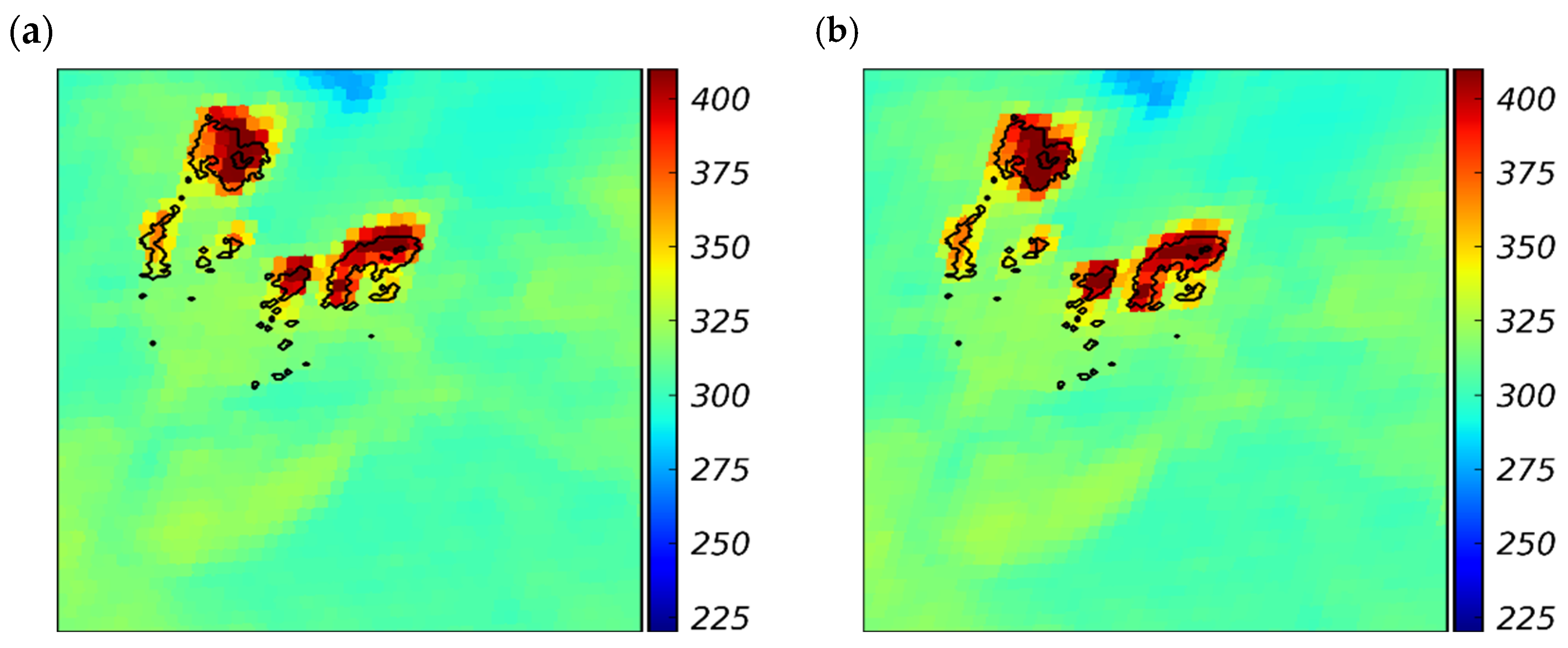
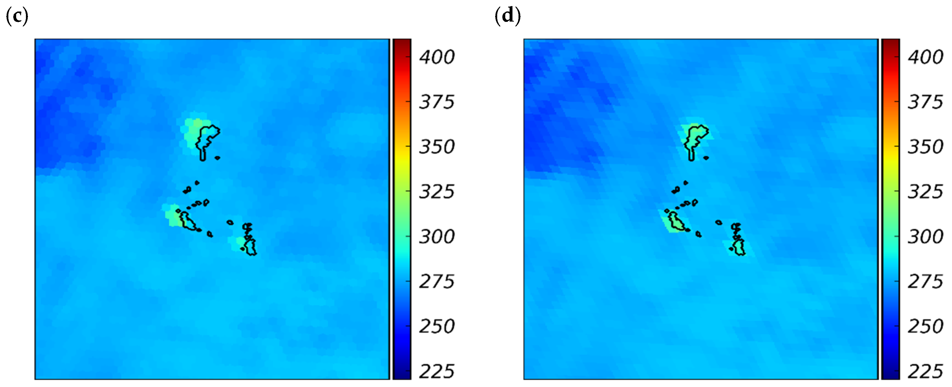
This appendix provides additional visual results supporting the data preprocessing steps. It shows examples of GOES–VIIRS spatial misalignment before and after parallax correction. Figure A1 illustrates the spatial misalignment between GOES Band 7 BT and VIIRS active fire boundaries, along with the improvement achieved through orthorectification [20]. Figure A1a,b correspond to GOES-17, which exhibits a northeastward shift relative to VIIRS. Figure A1c,d correspond to GOES-16, which exhibits a northwestward shift. In both cases, orthorectification reduces spatial displacement.
Figure A1.
Effect of orthorectification on the spatial alignment between GOES and VIIRS observations. Panels (a,b) show the Dixie Fire observed by GOES-17 on 5 August 2021 at 21:12 UTC, centered at −121° and 40° N. Panels (c,d) show the Hermits Peak Fire observed by GOES-16 on 4 May 2022 at 08:54 UTC, centered at −105° and 35° N. Panels (a,c) show the original imagery and panels (b,d) show the orthorectified imagery. Color indicates brightness temperature retrieved from GOES and black contours indicate fire boundaries derived from VIIRS. In the original imagery the GOES hot pixels are offset from the VIIRS contours, and this offset is largely removed after orthorectification.
Appendix B. Segmentation and Regression Model Architecture
This appendix details the DL architectures used in our approach. Table A1 describes the UNet variant that generates pixel-wise fire maps, and Table A2 describes the UNet-based regression model that predicts z-score normalized BT along with per-image statistical parameters ( and ) needed to reconstruct full-scale temperature values.
Table A1.
Architecture of the UNet variant used for fire segmentation. The model maps a 3-channel GOES image of size h × w to a 1-channel fire probability map, with a final sigmoid activation constraining outputs to [0, 1]. In the table, “Conv2d (3→64)” denotes a convolutional layer with 3 input and 64 output channels, “×2” denotes the two consecutive convolutions of a DoubleConv block, and “ConvTranspose2d” denotes the transposed convolution used for upsampling in the decoder. “BatchNorm2d” follows every convolutional layer unless noted otherwise.
Table A2.
Architecture of the UNet variant used for regression. The model takes a 3-channel GOES input and predicts a z-score normalized BT map for each pixel, along with the per-image mean of BT. These statistical parameters enable reconstruction of full-scale temperature values in Kelvin during evaluation. In the table, “Conv2d (3→64)” denotes a 2D convolutional layer with 3 input channels and 64 output channels, and “×2” indicates two consecutive convolutional operations within a DoubleConv block. “FC” refers to a fully connected layer. Two parallel fully connected branches produce the per-image mean and standard deviation, respectively, with an exponential activation (“Exp.”) applied to the standard deviation branch to ensure positivity. BatchNorm2d follows each convolutional layer unless otherwise specified.
Appendix C. Formal Metric Definitions
Appendix C.1. Notation
Let denote the total number of test images. For each image , let denote the full set of pixel indices in image prior to applying the invalid-pixel mask, which indicates artifact-corrupted pixels, and let denote the set of valid pixels that remain after the mask is applied. Every pixel is associated with a reference segmentation label . Every valid pixel is in addition associated with a predicted segmentation probability , a reference BT , and a predicted BT , where all BT values are expressed in Kelvin. Predicted quantities are undefined on and are never evaluated there. For a finite set , denotes its cardinality, and denotes the indicator function, which equals 1 when its argument is true and 0 otherwise. Unless stated otherwise, a summation over the image index runs over all test images, that is . The set of fire-containing test images is defined as . For a threshold , the hard segmentation prediction is . The same notation is applied to the validation set. In particular , , and carry the same meaning for validation images, and denotes the set of fire-containing validation images defined analogously to . The per-image confusion counts at threshold are defined as follows.
Appendix C.2. Fire Segmentation Metrics
AP is computed as the weighted mean of the Precision values attained at successive thresholds, where the weight assigned to each threshold is the increment in Recall achieved at that threshold. The per-image confusion counts defined in Appendix C.1 are aggregated globally across all valid pixels of all test images, including images that contain no annotated fire pixels, as follows.
At each threshold , Precision and Recall are defined as follows.
The Precision-Recall curve is anchored at zero Recall by an additional point that lies above every observed probability, for which = 0 and = 1 by convention. This point contributes no term to the sum below because the weight of index multiplies for ≥ 1. For every with ≥ 1 the denominator of is strictly positive because at least one pixel attains that probability, and the denominator of is strictly positive because the test set contains at least one annotated fire pixel.
where is the set of distinct predicted probabilities observed over all valid pixels of all test images, sorted in decreasing order so that Recall increases with . For the AP computation only, the hard prediction is taken as so that Recall reaches unity at the smallest observed probability, which is the convention adopted by the standard implementation used here, whereas all threshold-dependent metrics reported at use the strict inequality of Appendix C.1. This choice of grid makes AP exact in the sense that no interpolation between thresholds is required, and it reproduces the value returned by the standard implementation of AP. When AP is reported for a subset of test images grouped by annotated fire size, the global confusion counts are aggregated over the valid pixels of the images in that subset only, and the threshold grid is rebuilt from the probabilities observed within that subset. AP is undefined for the group of images that contain no annotated fire pixel because Recall is undefined there.
The operating threshold is selected on the validation set by maximizing the macro-averaged IoU over the fire-containing validation images introduced in Appendix C.1, that is
where the objective is a piecewise constant function of , so it is maximized over a finite grid of candidate thresholds rather than over the full interval. This grid is built in two stages. A coarse grid of 20 equally spaced values on the open interval is scanned first, and the three highest-scoring values are then searched over a local grid of 20 values within one coarse step on either side, so that contains 80 candidates at most. The denominator of the IoU is strictly positive for every because such an image contains at least one annotated fire pixel.
IoU, Precision, Recall, and F1 score are then computed at on the test set. The single obtained on the validation set is used for every threshold-dependent quantity reported in this study, including the image-level metrics defined below and every metric reported for a subset of test images grouped by annotated fire size, so no threshold is re-tuned per group. Per-image Precision, Recall, and F1 score are defined as follows.
The denominator of vanishes when the model predicts no fire pixel in image , and in that case is defined to be 0. Each metric is then macro-averaged over , the set of fire-containing test images. The averaging is shown below for IoU, and Precision, Recall, and F1 are averaged in the same manner.
For image-level metrics, an image is classified as fire-positive if at least one valid pixel exceeds . Formally, let . The invalid-pixel mask never removes every pixel of a test image, so is non-empty and the maximum is well defined for every . Image-level metrics are evaluated against the annotated reference before the invalid-pixel mask is applied, so let denote the set of images containing at least one annotated fire pixel, so that . This set is used because an image whose annotated fire pixels are all removed by the mask still represents a fire scene at the image level, whereas its pixel-level metrics are undefined. In this study = 1001, = 482 and = 481, the difference being a single test image in which every annotated fire pixel falls under the invalid-pixel mask. Then, the image-level omission error rate (OER) and false positive rate (FPR) are defined as follows.
Appendix C.3. BT Regression Metrics
For each image , let and denote the fire-pixel and background-pixel subsets, respectively. is computed only over images where is non-empty. The three RMSE metrics are defined as follows.
Appendix D. Details of Loss Functions
This appendix presents the details of the segmentation loss function. The study addresses the severe class imbalance caused by the small number of active fire pixels relative to the background. To address this, six loss functions are considered in the ablation study, each chosen for its ability to handle data sparsity, class imbalance, or limited spatial overlap. In addition to the BCE loss defined in Equation (6), other considered loss functions include the Focal loss, Combo loss, Jaccard loss, Tversky loss, and Focal Tversky loss. The goal of this evaluation is to determine which loss formulation provides more accurate localization of fire pixels. A smoothing constant of 1.0 × 10⁻⁶ is added to the numerator and the denominator of the region-based losses, which are computed per image and then averaged over the batch.
Focal loss integrates two key mechanisms into the BCE loss to better address the challenges of fire segmentation, namely a class weighting mechanism and a hard examples focusing mechanism [29]. These mechanisms are controlled by the hyperparameters and , respectively. The class weighting mechanism, governed by (ranging from 0 to 1), adjusts the relative importance of fire (foreground) and background pixels, where a higher assigns greater weight to fire pixels and a smaller assigns greater weight to background pixels. The focus on hard examples mechanism, controlled by , reduces the contribution of well-classified pixels (those where is close to the true label) by downweighting their loss using a modulating factor or . This shifts the training focus toward hard-to-classify pixels, such as low-intensity or small fires, which are often misclassified due to their similarity to background. Compared to standard BCE, which treats all pixels equally, Focal loss emphasizes learning from rare and hard-to-classify examples, making it particularly effective for tasks with high class imbalance and ambiguous boundaries. In practice, and interact with each other because the modulating factor already suppresses the contribution of the abundant and well-classified background pixels, which reduces the need for a large . Following the setting reported by Lin et al. [29], we use = 0.25. We set = 1, since a stronger focusing term was not found to be beneficial.
Combo loss [30] is formulated as a weighted sum of modified binary cross-entropy (MBCE) and Dice loss [31] to combine their complementary strengths as shown in Equation (A24). The MBCE component formulated in Equation (A22) introduces a weighting factor to address class imbalance by adjusting the relative importance of foreground/fire and background/Non-Fire terms. This loss provides a smooth gradient behavior, meaning it changes gradually with respect to the model’s predictions, which helps the model train steadily and avoid unstable jumps. Dice loss in Equation (A23), a special case of the Tversky loss in Equation (A26) with = = 0.5, enhances the learning signal from overlapping regions by weighting the intersection twice in the numerator. This property makes Dice loss particularly effective for segmenting small or sparse regions, such as active-fire pixels. This gives Dice a high sensitivity to spatial overlap, encouraging precise localization. By combining MBCE’s smooth gradient behavior with Dice loss’s sensitivity to spatial overlap, Combo loss balances pixel-wise classification and region-level accuracy. The hyperparameter controls the contribution of each component. In this study, = 0.25 and = 0.75 are used.
The Jaccard loss defined in the following equation is a region-based loss function that directly optimizes the IoU score, encouraging better overlap between predicted and reference binary masks and improving spatial alignment.
In the above equation, the numerator represents the soft intersection between the predicted fire probabilities and the reference mask, which reduces to the number of pixels correctly identified as fire when the predictions are binary. The denominator includes the union of the predicted and reference regions. Specifically, it sums all pixels identified as fire by either the reference or the model, then subtracts the overlapping pixels to avoid double-counting. In effect, this means the model is rewarded when it accurately predicts fire pixels and penalized when it predicts too many false positives (FP) or misses fire pixels.
Tversky loss [32], as defined in Equation (A26), is a region-based loss function and generalizes the Dice loss by introducing adjustable weights to balance the importance of FP and false negatives (FN). This flexibility is important in fire segmentation tasks, where missing active fire pixels (FN) can have serious consequences. The Tversky loss can be calculated as follows.
where and weight FP and FN respectively under the constraint + = 1, following the original formulation of Salehi et al. [32]. The second term in the denominator increases when the model predicts fire where there is no fire (FP), while the third term increases when it fails to predict fire where it exists (FN). A larger therefore penalizes FN more strongly and encourages the model to delineate more fire pixels at the risk of overprediction. Since missed active fires delay response and increase damage, we set = 0.25 and = 0.75 to prioritize Recall over Precision.
Finally, Focal Tversky loss [33] builds on Tversky loss by adding a focusing parameter , which acts as a spotlight, intensifying the penalty for incorrect or uncertain predictions while dimming the influence of easy, confidently correct ones. By raising the Tversky loss to the power of > 1, the loss becomes more sensitive to pixels where the model struggles such as small, faint, or partially resolved fires, forcing the network to pay more attention to these cases during training. In this study, we set = 2. The Focal Tversky loss is defined as follows.
Appendix E. Detailed Ablation Results
This appendix provides additional quantitative and qualitative results of the ablation studies. It reports visual comparisons and explains how each tested option, namely the loss function, loss-weight hyperparameters, and the background setting, affects the model performance.
Appendix E.1. Segmentation Loss Function
Figure A2 shows segmentation predictions from each loss function for three representative wildfires, Lost Lake (2022-05-27, Small, 493 fire pixels), Luna (2020-10-18, Medium, 1095 fire pixels), and Sugar (2021-07-10, Large, 5086 fire pixels), with corresponding IoU scores shown below. Table A3 provides aggregate performance stratified by fire size category, Small (1–500 fire pixels), Medium (501–2000 fire pixels), and Large (more than 2000 fire pixels).
BCE achieves IoU scores of 0.397, 0.552, and 0.565 for Lost Lake, Luna, and Sugar. Although its Lost Lake performance is among the lowest of all methods, with only Tversky loss lower at 0.377, BCE produces spatially compact fire regions that closely match the VIIRS reference on Medium and Large events. Table A3 confirms this trend, as BCE achieves the highest AP in every size category, 0.235 for Small, 0.441 for Medium, and 0.444 for Large fires. Focal loss achieves moderate performance across all three events, with IoU scores of 0.454, 0.442, and 0.548, outperforming BCE on Lost Lake but falling behind on Medium and Large events.
Combo loss demonstrates balanced IoU across events at 0.463, 0.528, and 0.506 for Lost Lake, Luna, and Sugar, avoiding extreme over- or underprediction, but fails to capture finer structural details at fire boundaries, particularly the thinner peripheral extensions in the Sugar case. In Table A3, Combo loss achieves the highest IoU of 0.124 for Small fires, yet its AP remains below BCE in all categories. Jaccard loss achieves the highest individual IoU among all methods on Luna at 0.608 and remains competitive on Lost Lake at 0.459, though its advantage narrows on the spatially complex Sugar fire at 0.510. Table A3 also shows Jaccard loss achieving competitive IoU for Medium fires at 0.299 and the highest Precision for Medium at 0.463 and Large fires at 0.459, though its AP stays substantially lower than BCE across all categories, 0.136 for Small, 0.255 for Medium, and 0.272 for Large, limiting its suitability under class-imbalanced conditions.
Tversky loss and Focal Tversky loss yield competitive per-event IoU scores. In Figure A2, Tversky loss yields IoU values of 0.377, 0.473, and 0.509, while Focal Tversky loss yields 0.461, 0.499, and 0.503 for Lost Lake, Luna, and Sugar, respectively. Despite these values, both Tversky-based losses fall below BCE on the Luna and Sugar events, and their Sugar predictions remain compact and miss the peripheral extensions of the reference. In Table A3, however, Tversky loss achieves the highest Recall for Medium fires at 0.626 and Large fires at 0.625, as well as the highest IoU of 0.321 and F1 of 0.465 for Large fires, while Focal Tversky loss achieves the highest IoU of 0.302 and F1 of 0.443 for Medium fires. Notwithstanding these aggregate strengths, both Tversky-based methods yield substantially lower AP values than BCE across all size categories, indicating weaker probability ranking across decision thresholds.
Given that the segmentation task is inherently class-imbalanced, AP is a more informative metric than IoU. BCE achieves the highest AP among all loss functions at 0.368 for Overall (Table 5) and is therefore selected as the preferred loss function for the final segmentation model.
Table A3.
Ablation study on loss functions for fire segmentation. Six loss functions are evaluated on the test set across five metrics for each fire size category, namely Small (1–500 px), Medium (501–2000 px), and Large (>2000 px), where px denotes the number of fire pixels. Results are the mean ± standard deviation over three seeds, with the best value per metric shown in bold.
Figure A2.
Qualitative comparison of segmentation outputs under different loss functions. Columns correspond to six loss functions and Reference. Rows correspond to three wildfire events, namely Lost Lake (Small), Luna (Medium), and Sugar (Large). Brightness temperature (BT) in fire regions is derived from the same regression model which is trained by (, ) = (0.25, 0.75) and background BT = 240 K.
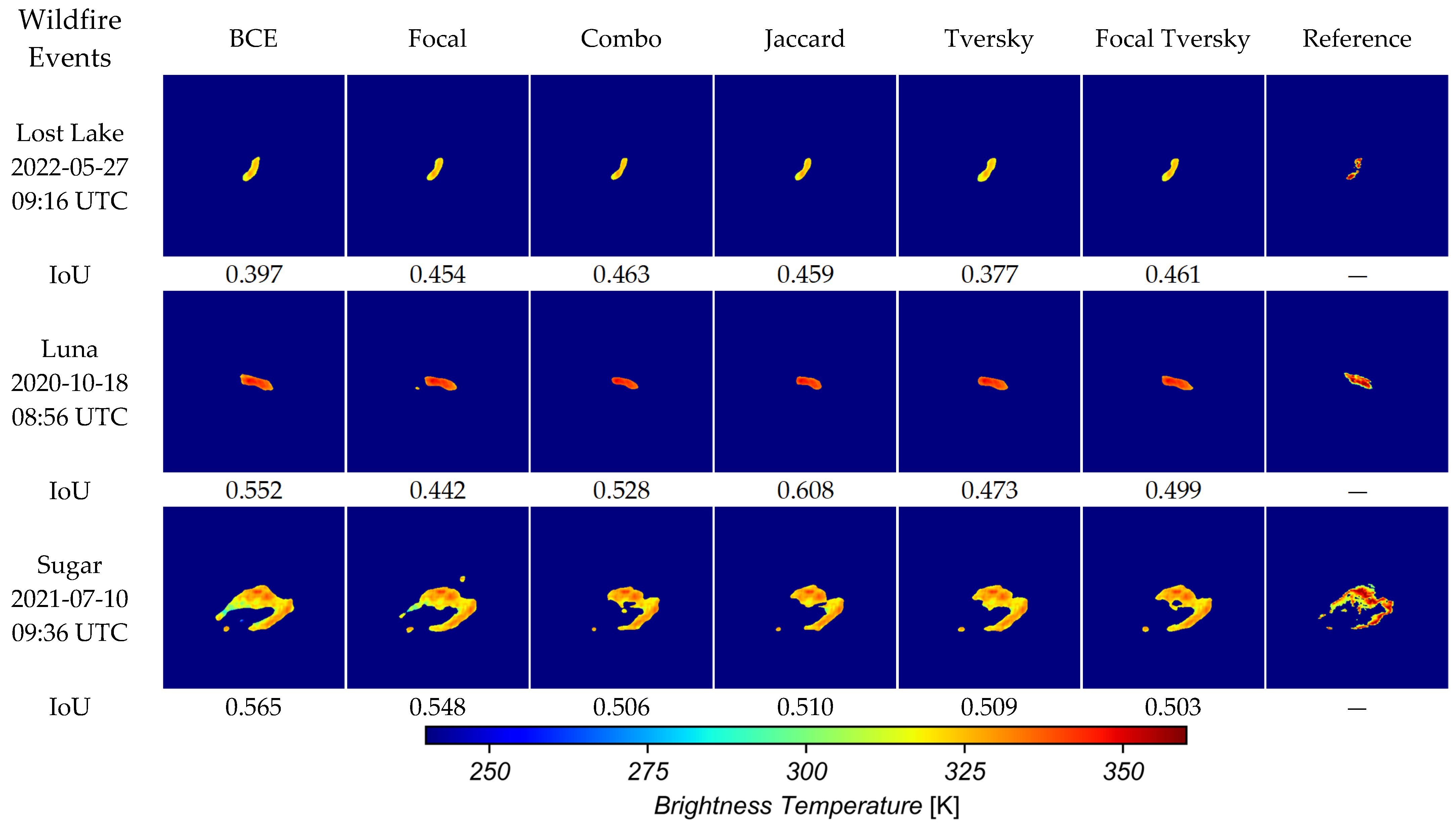
Appendix E.2. Loss Weight Hyperparameters
Table A4 and Figure A3 together characterize the effect of varying the loss weight hyperparameters and on reconstruction quality. Three configurations are evaluated, namely (, ) = (0.75, 0.25), (0.50, 0.50), and (0.25, 0.75). Table A4 reports , , and across fire size categories as the mean and standard deviation over three random seeds. Figure A3 presents qualitative sub-pixel estimation outputs for three representative wildfire events, Lost Lake (2022-05-27, Small, 493 fire pixels), Luna (2020-10-18, Medium, 1095 fire pixels), and Sugar (2021-07-10, Large, 5086 fire pixels).
Table A4 reveals a consistent trade-off between overall reconstruction accuracy and fire region fidelity. The background-weighted configuration achieves the lowest and across every category, with of 4.08 K for Small, 7.62 K for Medium, and 13.89 K for Large fires, reflecting the dominant influence of background pixels in scene-level metrics. However, it consistently yields the highest across all fire size categories at 56.77 K for Small, 37.10 K for Medium, and 36.65 K for Large fires, indicating substantially degraded fire region fidelity. Conversely, the fire-weighted configuration achieves the best in all three fire size categories at 24.11, 17.80, and 17.40 K for Small, Medium, and Large fires, respectively. These values decrease monotonically with fire size, indicating that fire region reconstruction is intrinsically more accurate when more fire pixels are available. The improvement relative to the background-weighted configuration is nevertheless present in every category, with the largest gain of 32.66 K for Small fires. This gain in fire region accuracy is accompanied by a substantial increase in and , reflecting degraded background reconstruction. The balanced configuration achieves intermediate values throughout, without incurring the substantial penalty of the fire-weighted setting.
A noteworthy pattern emerges when comparing Non-Fire and fire scene categories. Non-Fire scenes serve as a reference for pure background reconstruction. Under the background-weighted configuration, the Non-Fire is 3.38 K, whereas the corresponding in fire scenes is consistently higher and increases with fire size at 3.99, 7.37, and 13.56 K for Small, Medium, and Large fires, respectively. This degradation of background reconstruction in fire scenes is observed across all weight configurations, and the gap widens with fire size. This suggests that fire pixels adversely affect background reconstruction even under the background-weighted setting, likely because high-magnitude fire pixels near boundaries cause the model to overestimate BT in adjacent regions. These trends are consistent with the qualitative results in Figure A3. The background-weighted configuration produces spatially variable fire regions, yielding the highest per-event across all three events at 15.89 K for Lost Lake, 26.57 K for Luna, and 27.58 K for Sugar. Increasing the fire weight to 0.50 reduces substantially for Luna at 22.25 K and Sugar at 19.24 K, and achieves the lowest value for Lost Lake at 14.72 K. The fire-weighted configuration further improves performance for Luna and Sugar at 18.74 and 12.80 K, respectively, with predicted fire regions most accurately matching the VIIRS reference.
Overall, increasing improves fire region fidelity, while increasing yields lower background errors. The balanced configuration remains competitive for Small events such as Lost Lake, whereas the fire-weighted configuration is most effective for larger and spatially complex fires, as confirmed by both the aggregate statistics and Figure A3.
Table A4.
Ablation study on loss weight hyperparameters (, ), where and denote the weights applied to background and fire pixels in the loss function, respectively. Results are reported for Small (1–500 px), Medium (501–2000 px), Large (>2000 px), and Non-Fire categories, where px denotes the number of fire pixels, as the mean ± standard deviation over three seeds. The best result for each metric is highlighted in bold.
Figure A3.
Qualitative comparison of sub-pixel estimation outputs under varying weight settings. Columns correspond to weight combinations = (0.75, 0.25), (0.50, 0.50), and (0.25, 0.75), as well as Reference. Rows correspond to three wildfire events, namely Lost Lake (Small), Luna (Medium), and Sugar (Large). Fire segmentation masks are derived from the BCE-based segmentation output.
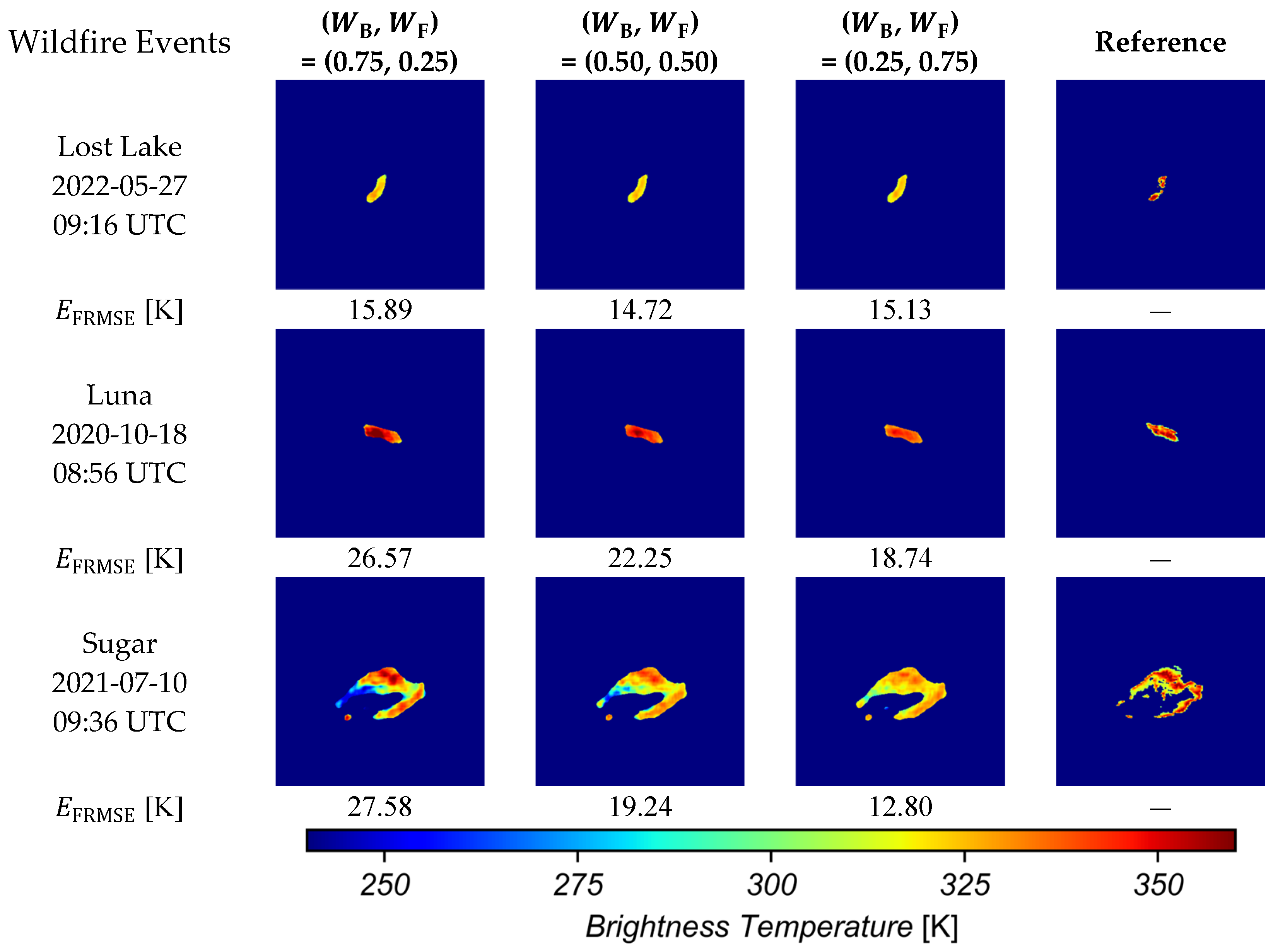
Appendix E.3. Background Brightness Temperature
Figure A4 presents qualitative sub-pixel estimation outputs under four background BT settings of 0 K, 220 K, 240 K, and 260 K, alongside the VIIRS reference for three representative wildfire events, Lost Lake (2022-05-27, Small, 493 fire pixels), Luna (2020-10-18, Medium, 1095 fire pixels), and Sugar (2021-07-10, Large, 5086 fire pixels). Overall, increasing the background BT from 0 K to 260 K leads to a consistent reduction in , as evidenced by the Luna event decreasing from 23.34 K to 17.40 K and the Sugar event decreasing dramatically from 34.71 K to 12.59 K. However, the Lost Lake event does not follow this trend, exhibiting relatively stable and low values across all background BT settings with a variation of only approximately 1.4 K, which may be attributable to its small spatial extent and simple elongated geometry rendering the estimation less sensitive to background thermal context. Within the physically plausible range of 220 K to 260 K, values stabilize across all events.
Table A5 quantitatively corroborates the trends observed in Figure A4 across all fire size categories. All metrics decrease monotonically as the background BT increases from 0 K to 280 K, with the most substantial improvement occurring between 0 K and 220 K. For example, for the Large fire drops from 117.50 K at 0 K to 48.15 K at 220 K, while the subsequent decrease from 220 K to 280 K amounts to approximately 28 K. Larger fire events consistently exhibit higher absolute errors at low background BT settings, suggesting that fires with greater spatial extent are more adversely affected by an unrealistic thermal background, a finding consistent with the qualitative observations in Figure A4. While these results suggest that a higher background BT of 280 K yields the lowest estimation errors across all categories, this trend must be interpreted with caution. As discussed in Section 4.3.3, 280 K exceeds the coldest annotated fire pixels in the training set and is therefore physically inconsistent, whereas both 260 K and 240 K remain below the observed fire pixel range. We adopt 240 K because it preserves the wider separation from the fire BT distribution, and we note that the difference in accuracy with respect to 260 K is modest.
Figure A4.
Qualitative comparison of sub-pixel estimation outputs under varying background brightness temperature (BT) settings. Columns correspond to background BT values of 0 K, 220 K, 240 K, and 260 K, as well as Reference. Rows correspond to three wildfire events, namely Lost Lake (Small), Luna (Medium), and Sugar (Large). The values listed below each panel denote the per-event [K]. Fire segmentation masks are derived from the BCE-based segmentation output. The background BT setting of 280 K was excluded from this comparison because it is physically inconsistent.
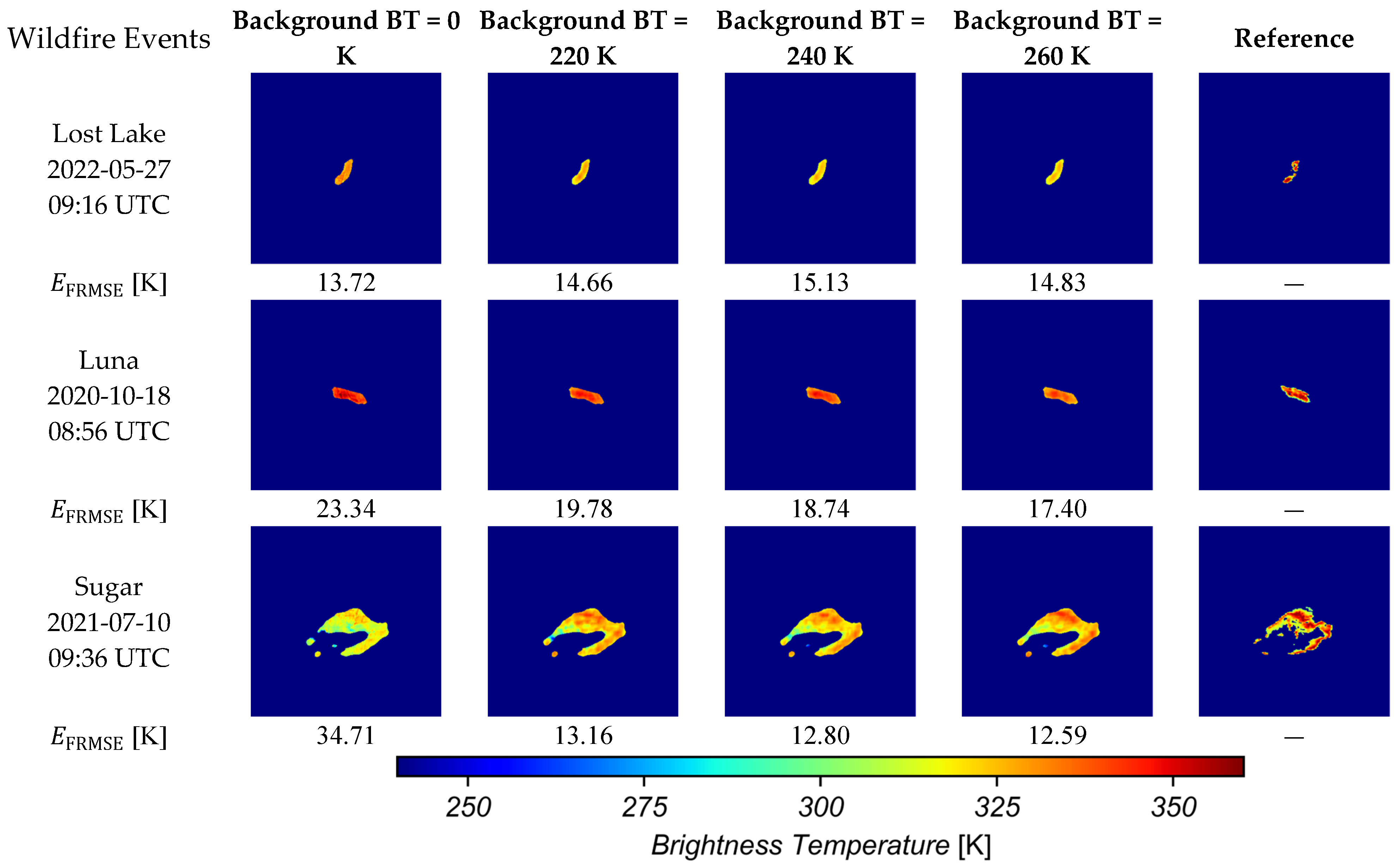
Table A5.
Ablation study on the background brightness temperature (BT). Results are reported for Small (1–500 px), Medium (501–2000 px), Large (>2000 px), and Non-Fire categories, where px denotes the number of fire pixels, as the mean ± standard deviation over three seeds.
Appendix F. Wildfire Event List
Table A6 summarizes the wildfire events used in this study. It provides the fire event name, MTBS ID, total burned area, geographic coordinates, time range, and splits for each fire included in the dataset.
Table A6.
Metadata for wildfire events in the dataset, including MTBS identifiers (name and ID), burned area in acres, geographic coordinates in degrees longitude and latitude, active burn period start and end dates, and dataset split assignment. Coordinates denote the ROI center. Events in close spatial and temporal proximity share a common ROI and therefore share identical center coordinates. One acre is approximately equal to 0.4 hectares. Two events, SMOKEHOUSE CREEK and GRAPE VINE CREEK, are each represented by two rows (suffixed 1 and 2), sharing a single MTBS ID but corresponding to spatially distinct burn centers that were processed as separate samples. As a result, the table contains 259 rows corresponding to 257 unique MTBS events, and the 83 test rows correspond to 81 unique test events.
References
- National Interagency Coordination Center. Wildland Fire Summary and Statistics Annual Report 2023; National Interagency Coordination Center: Boise, ID, USA, 2024.
- Prins, E.M.; Menzel, W.P. Geostationary Satellite Detection of Biomass Burning in South America. Int. J. Remote Sens. 1992, 13, 2783–2799. [Google Scholar] [CrossRef] [Scilit]
- Prins, E.M.; Menzel, W.P. Trends in South American Biomass Burning Detected with the GOES Visible Infrared Spin Scan Radiometer Atmospheric Sounder from 1983 to 1991. J. Geophys. Res. Atmos. 1994, 99, 16719–16735. [Google Scholar] [CrossRef] [Scilit]
- Prins, E.M.; Feltz, J.M.; Menzel, W.P.; Ward, D.E. An Overview of GOES-8 Diurnal Fire and Smoke Results for SCAR-B and 1995 Fire Season in South America. J. Geophys. Res. Atmos. 1998, 103, 31821–31835. [Google Scholar] [CrossRef] [Scilit]
- Zhao, Y.; Ban, Y. GOES-R Time Series for Early Detection of Wildfires with Deep GRU-Network. Remote Sens. 2022, 14, 4347. [Google Scholar] [CrossRef] [Scilit]
- Koltunov, A.; Ustin, S.L.; Prins, E.M. On Timeliness and Accuracy of Wildfire Detection by the GOES WF-ABBA Algorithm over California during the 2006 Fire Season. Remote Sens. Environ. 2012, 127, 194–209. [Google Scholar] [CrossRef] [Scilit]
- Koltunov, A.; Ustin, S.L.; Quayle, B.; Schwind, B. GOES Early Fire Detection (GOES-EFD) System Prototype. In Proceedings of the ASPRS 2012 Annual Conference, Sacramento, CA, USA, 19–23 March 2012; pp. 19–23. [Google Scholar]
- Schmidt, C.C.; Hoffman, J.; Prins, E.M.; Lindstrom, S. GOES-R Advanced Baseline Imager (ABI) Algorithm Theoretical Basis Document for Fire/Hot Spot Characterization, Version 2.7; NESDIS, NOAA: Silver Spring, MD, USA, 2020.
- Toan, N.T.; Thanh Cong, P.; Viet Hung, N.Q.; Jo, J. A Deep Learning Approach for Early Wildfire Detection from Hyperspectral Satellite Images. In Proceedings of the 2019 7th International Conference on Robot Intelligence Technology and Applications (RiTA); IEEE: Daejeon, Republic of Korea, 2019; pp. 38–45. [Google Scholar]
- Malik, A.; Jalin, N.; Rani, S.; Singhal, P.; Jain, S.; Gao, J. Wildfire Risk Prediction and Detection Using Machine Learning in San Diego, California. In Proceedings of the 2021 IEEE SmartWorld, Ubiquitous Intelligence & Computing, Advanced & Trusted Computing, Scalable Computing & Communications, Internet of People and Smart City Innovation (SmartWorld/SCALCOM/UIC/ATC/IOP/SCI); IEEE: Atlanta, GA, USA, 2021; pp. 622–629. [Google Scholar]
- Badhan, M.; Shamsaei, K.; Ebrahimian, H.; Bebis, G.; Lareau, N.P.; Rowell, E. Deep Learning Approach to Improve Spatial Resolution of GOES-17 Wildfire Boundaries Using VIIRS Satellite Data. Remote Sens. 2024, 16, 715. [Google Scholar] [CrossRef] [Scilit]
- Schroeder, W.; Giglio, L.; Hall, J. Collection 2 Visible Infrared Imaging Radiometer Suite (VIIRS) 375-m Active Fire Product User’s Guide Version 1.0; NASA: Washington, DC, USA, 2024.
- Schmit, T.J.; Griffith, P.; Gunshor, M.M.; Daniels, J.M.; Goodman, S.J.; Lebair, W.J. A Closer Look at the ABI on the GOES-R Series. Bull. Am. Meteorol. Soc. 2017, 98, 681–698. [Google Scholar] [CrossRef] [Scilit]
- Giglio, L.; Schroeder, W.; Csiszar, I.; Tsidulko, M. Algorithm Theoretical Basis Document for NOAA NDE VIIRS Active Fire, Version 2.6; NOAA: College Park, MD, USA, 2016.
- Schroeder, W.; Giglio, L. Visible Infrared Imaging Radiometer Suite (VIIRS) 375 m Active Fire Detection and Characterization Algorithm Theoretical Basis Document 1.0; University of Maryland: College Park, MD, USA, 2016. [Google Scholar]
- Schroeder, W.; Oliva, P.; Giglio, L.; Csiszar, I.A. The New VIIRS 375 m Active Fire Detection Data Product: Algorithm Description and Initial Assessment. Remote Sens. Environ. 2014, 143, 85–96. [Google Scholar] [CrossRef] [Scilit]
- NOAA Earth from Orbit: NOAA’s GOES-18 Is Now GOES West. Available online: https://www.nesdis.noaa.gov/news/earth-orbit-noaas-goes-18-now-goes-west (accessed on 28 June 2026).
- Barducci, A.; Guzzi, D.; Marcoionni, P.; Pippi, I. Comparison of Fire Temperature Retrieved from SWIR and TIR Hyperspectral Data. Infrared Phys. Technol. 2004, 46, 1–9. [Google Scholar] [CrossRef] [Scilit]
- Eidenshink, J.; Schwind, B.; Brewer, K.; Zhu, Z.-L.; Quayle, B.; Howard, S. A Project for Monitoring Trends in Burn Severity. Fire Ecol. 2007, 3, 3–21. [Google Scholar] [CrossRef] [Scilit]
- Pestana, S.; Lundquist, J.D. Evaluating GOES-16 ABI Surface Brightness Temperature Observation Biases over the Central Sierra Nevada of California. Remote Sens. Environ. 2022, 281, 113221. [Google Scholar] [CrossRef] [Scilit]
- Moritz, H. Geodetic Reference System 1980. Bull. Geod. 1980, 54, 395–405. [Google Scholar] [CrossRef] [Scilit]
- NASA SRTM. Shuttle Radar Topography Mission (SRTM) Global; NASA: Washington, DC, USA, 2013.
- European Space Agency. Copernicus Global Digital Elevation Model; European Space Agency: Paris, France, 2024. [Google Scholar]
- Ronneberger, O.; Fischer, P.; Brox, T. U-Net: Convolutional Networks for Biomedical Image Segmentation. In Proceedings of the Medical Image Computing and Computer-Assisted Intervention–MICCAI 2015; Springer: Berlin/Heidelberg, Germany, 2015; Volume 9351, pp. 234–241. [Google Scholar]
- Lim, B.; Son, S.; Kim, H.; Nah, S.; Lee, K.M. Enhanced Deep Residual Networks for Single Image Super-Resolution. In Proceedings of the IEEE Conference on Computer Vision and Pattern Recognition Workshops (CVPRW), Honolulu, HI, USA, 21–26 July 2017; pp. 1132–1140. [Google Scholar]
- Saito, T.; Rehmsmeier, M. The Precision-Recall Plot Is More Informative than the ROC Plot When Evaluating Binary Classifiers on Imbalanced Datasets. PLoS ONE 2015, 10, e0118432. [Google Scholar] [CrossRef] [Scilit]
- Wu, Z.; Gao, Y.; Li, L.; Xue, J.; Li, Y. Semantic Segmentation of High-Resolution Remote Sensing Images Using Fully Convolutional Network with Adaptive Threshold. Connect. Sci. 2019, 31, 169–184. [Google Scholar] [CrossRef] [Scilit]
- Kingma, D.P.; Ba, J. Adam: A Method for Stochastic Optimization. In Proceedings of the 3rd International Conference on Learning Representations, San Diego, CA, USA, 7–9 May 2015. [Google Scholar]
- Lin, T.-Y.; Goyal, P.; Girshick, R.; He, K.; Dollár, P. Focal Loss for Dense Object Detection. In Proceedings of the IEEE International Conference on Computer Vision (ICCV), Venice, Italy, 22–29 October 2017; pp. 2980–2988. [Google Scholar]
- Taghanaki, S.A.; Zheng, Y.; Zhou, S.K.; Georgescu, B.; Sharma, P.; Xu, D.; Comaniciu, D.; Hamarneh, G. Combo Loss: Handling Input and Output Imbalance in Multi-Organ Segmentation. Comput. Med. Imaging Graph. 2019, 75, 24–33. [Google Scholar] [CrossRef] [Scilit] [PubMed]
- Milletari, F.; Navab, N.; Ahmadi, S.A. V-Net: Fully Convolutional Neural Networks for Volumetric Medical Image Segmentation. In Proceedings of the 2016 Fourth International Conference on 3D Vision (3DV), Stanford, CA, USA, 25–28 October 2016; IEEE: New York, NY, USA, 2016; pp. 565–571. [Google Scholar]
- Salehi, S.S.M.; Erdogmus, D.; Gholipour, A. Tversky Loss Function for Image Segmentation Using 3D Fully Convolutional Deep Networks. In Proceedings of the Machine Learning in Medical Imaging (MLMI 2017); Springer: Berlin/Heidelberg, Germany, 2017; Volume 10541 LNCS, pp. 379–387. [Google Scholar]
- Abraham, N.; Khan, N.M. A Novel Focal Tversky Loss Function with Improved Attention U-Net for Lesion Segmentation. In Proceedings of the 2019 IEEE 16th International Symposium on Biomedical Imaging (ISBI 2019), Venice, Italy, 8–11 April 2019; IEEE: New York, NY, USA, 2019; pp. 683–687. [Google Scholar]
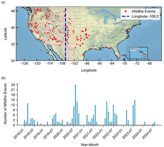
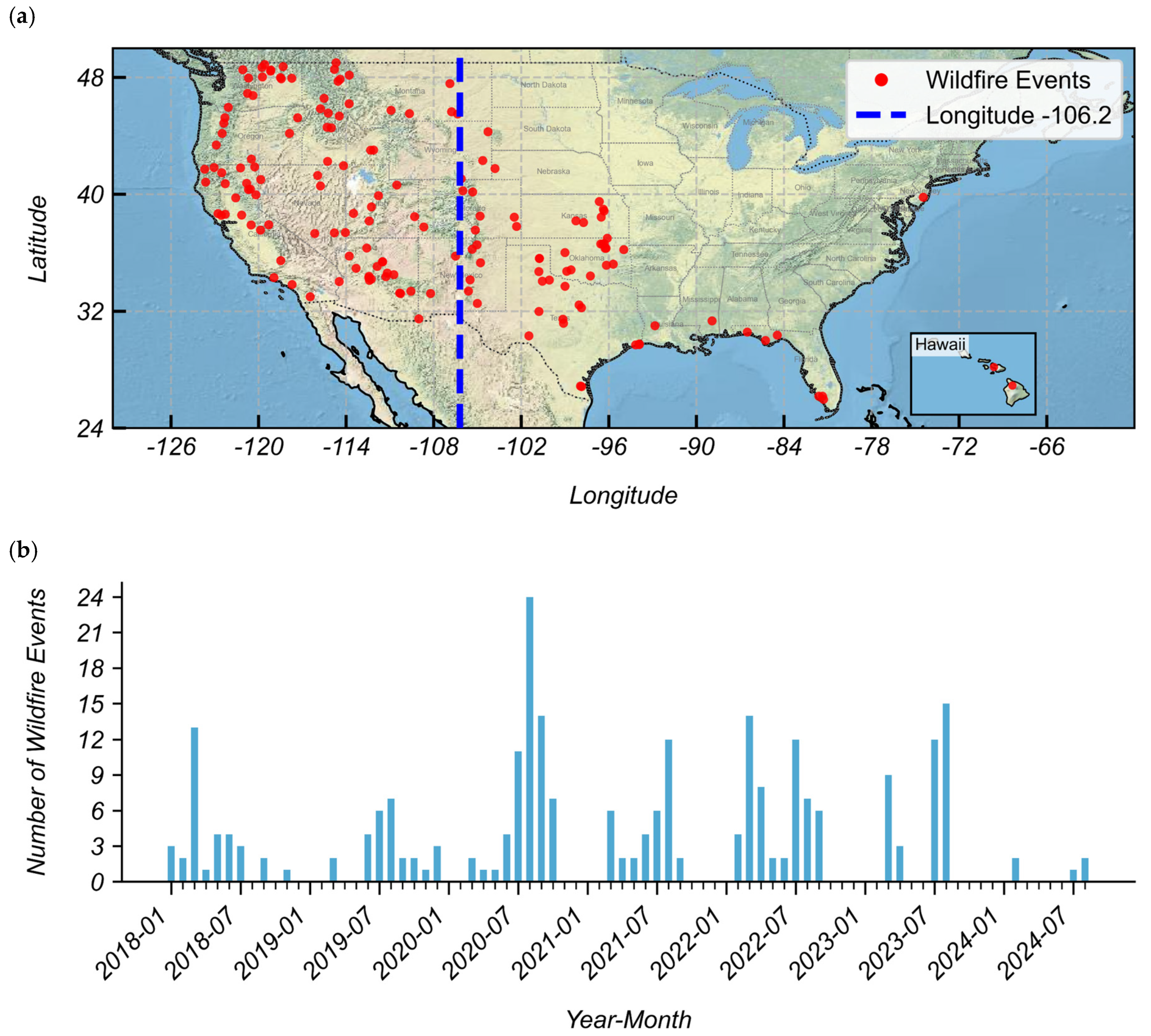
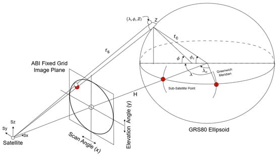
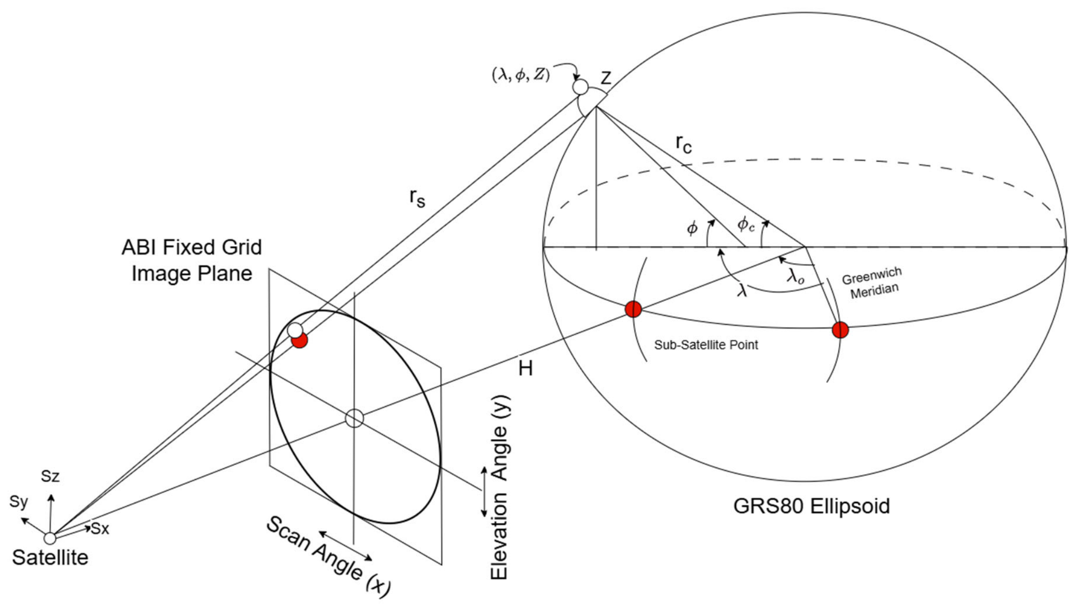
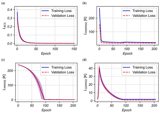
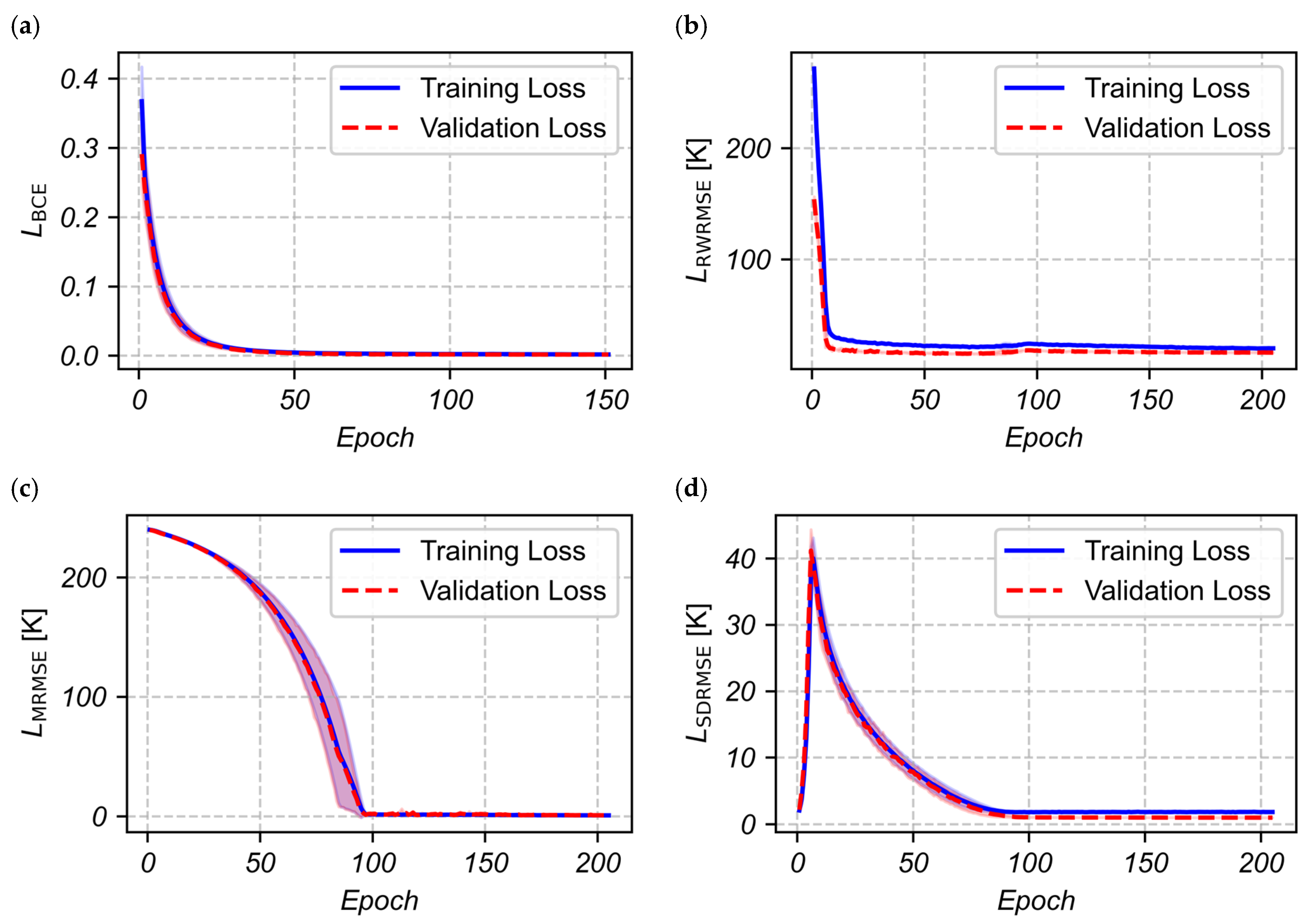
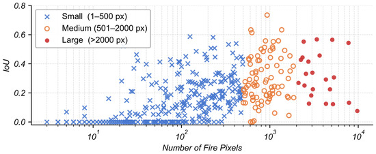
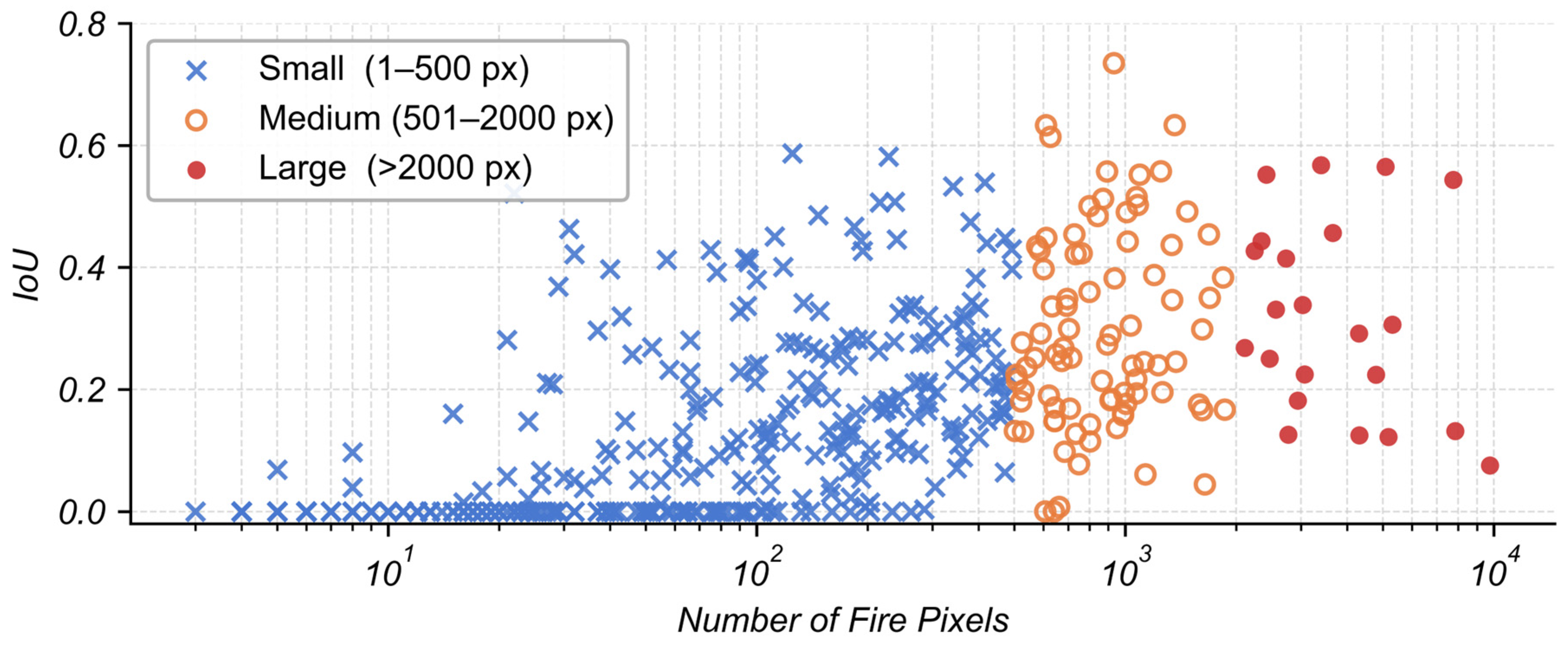
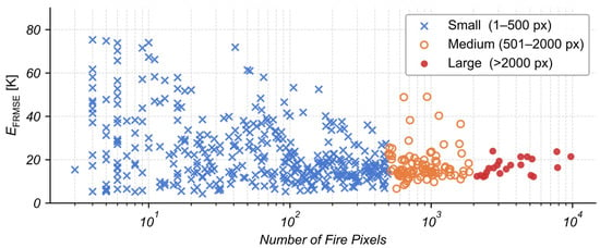
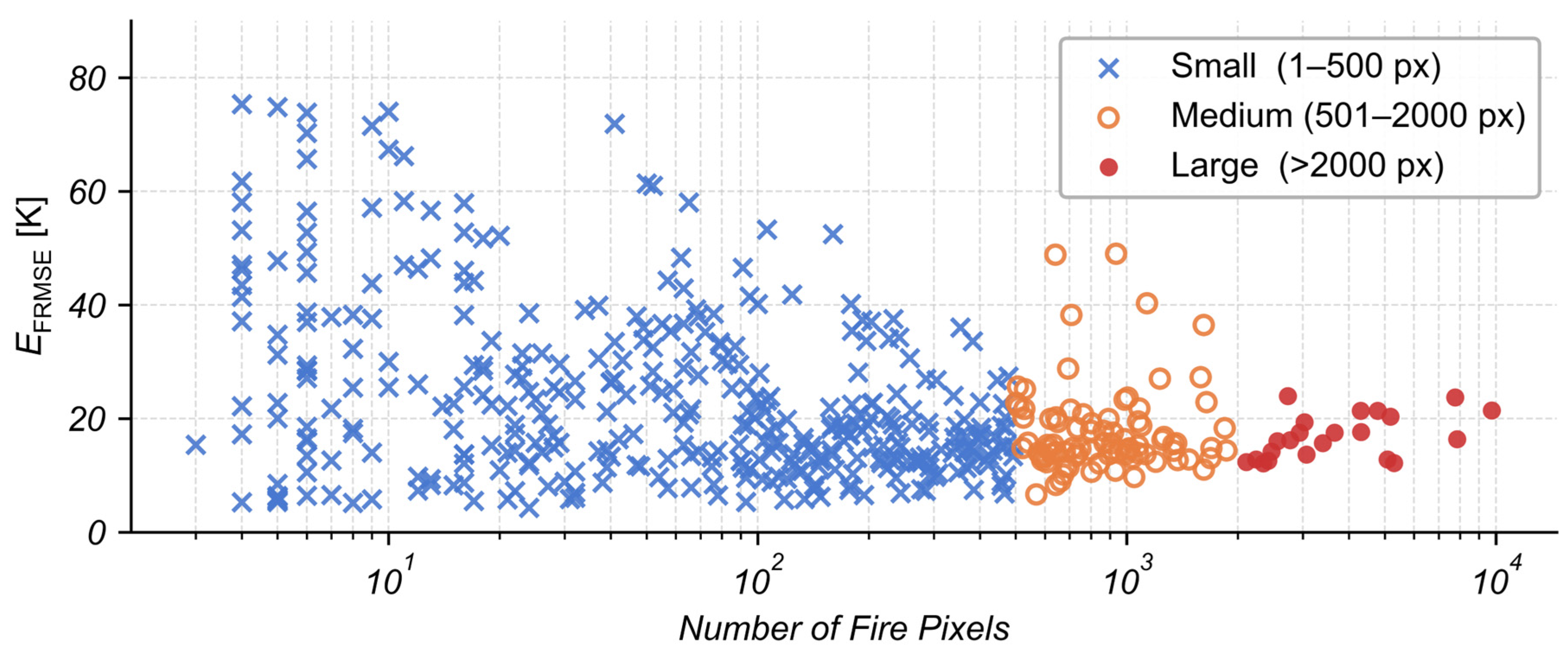
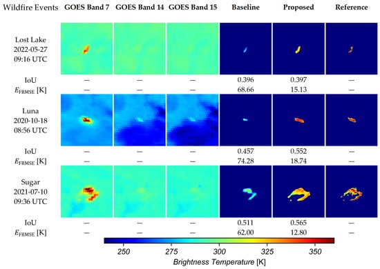
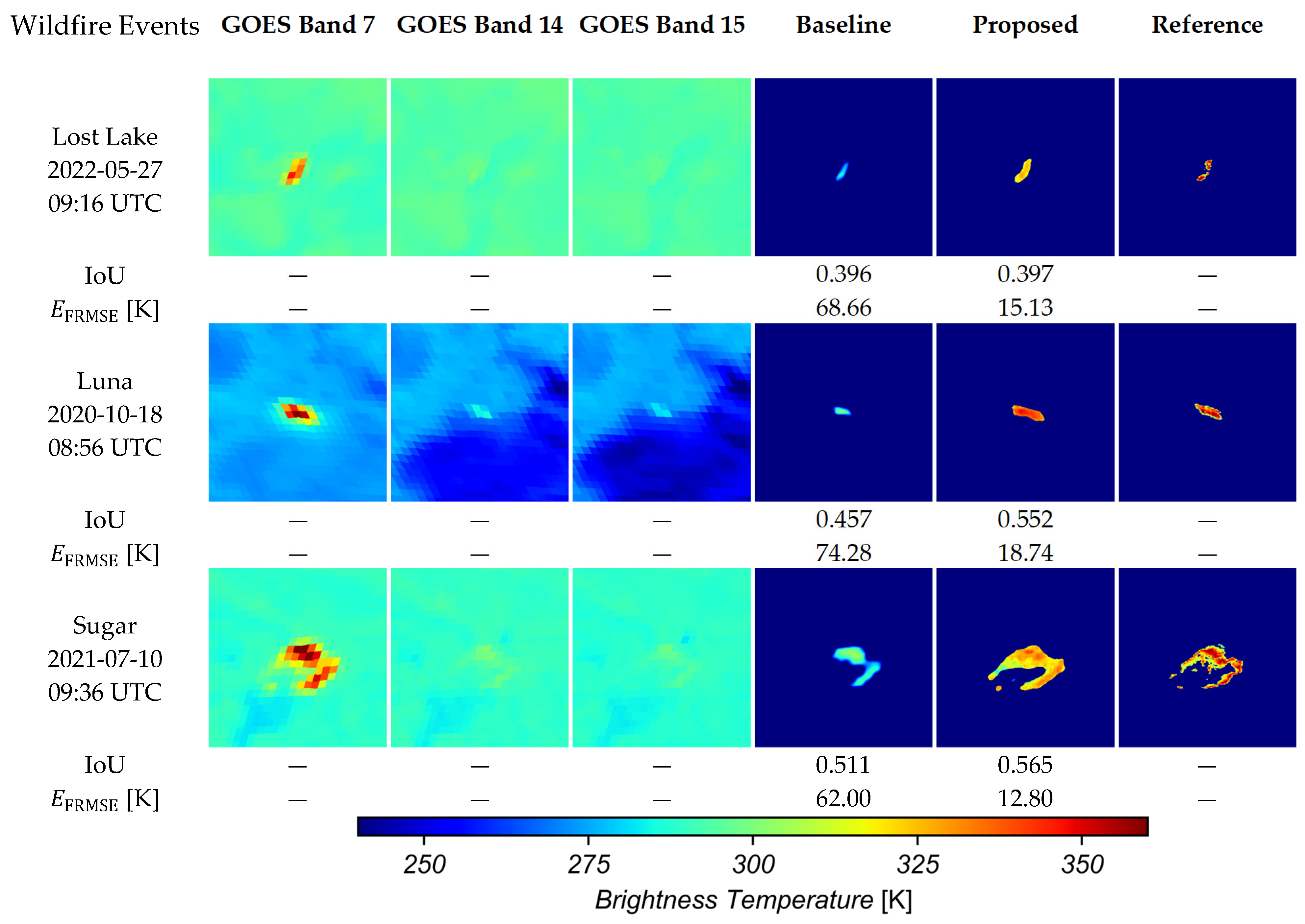
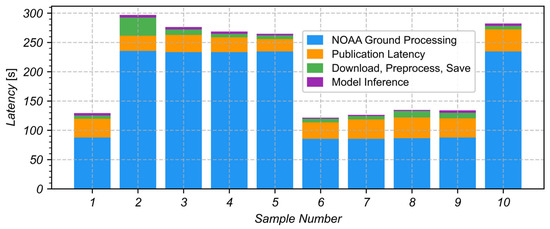
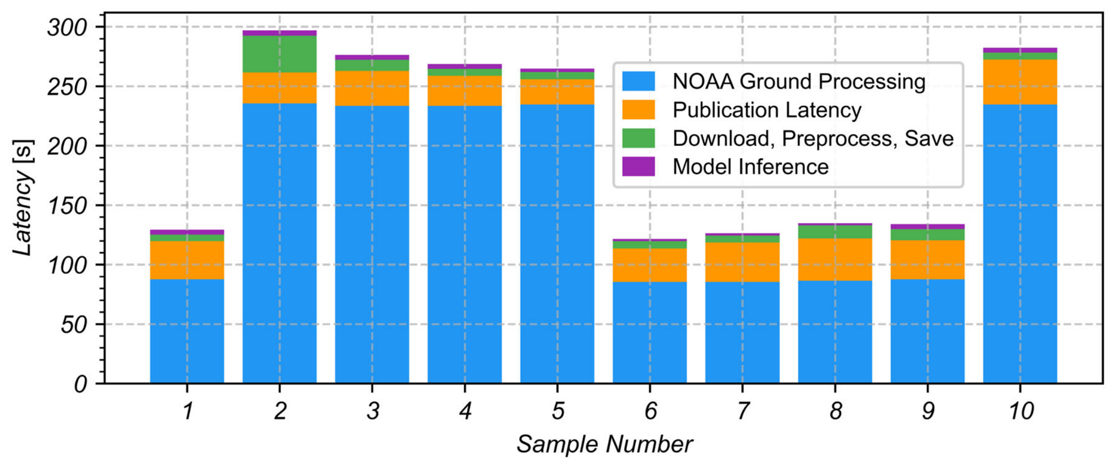

Disclaimer/Publisher’s Note: The statements, opinions and data contained in all publications are solely those of the individual author(s) and contributor(s) and not of MDPI and/or the editor(s). MDPI and/or the editor(s) disclaim responsibility for any injury to people or property resulting from any ideas, methods, instructions or products referred to in the content. |
© 2026 by the authors. Licensee MDPI, Basel, Switzerland. This article is an open access article distributed under the terms and conditions of the Creative Commons Attribution (CC BY) license.