


Abstract
Wildfire smoke contains complex mixtures of inorganic and organic species, yet metals in experimental smoke preparations are rarely quantified in a manner directly useful for toxicology. Here, an inductively coupled plasma–mass spectrometry (ICP-MS) workflow for multi-element analysis of bushfire smoke preparations was explored for use in future cell-based studies. The novel contribution is the integration of matrix-matched blank correction, near-LOD handling, micromolar unit conversion and multivariate visualisation into a reproducible workflow for preparation-specific smoke exposure characterisation. This study is an analytical-methods contribution that provides composition-based exposure-characterisation inputs for future toxicological and risk-assessment studies, rather than a direct assessment of biological toxicity or health risk. Eight case-study preparations were analysed: two laboratory-generated bushfire smoke stock solutions (BF#1, BF#2); four laboratory bushfire smoke filter extracts with dominant vegetation types of Eucalyptus, Pine, Banksia, and Mallee; and paired blue gum smoke chamber T- and G-phase samples, each with matched blanks. The workflow combined blank mapping and subtraction, handling of values near the limit of detection, and conversion of concentrations to blank-corrected micromolar units in analytical extracts. Major ions (Na, K, Ca, Mg, P, S) dominated the metal burden, redox-active metals (Al, Mn, Fe, Cu, Zn) were present at sub- to low-micromolar levels, and toxic metals (Pb, Cd) were generally low, with Pb elevated in one filter extract. Silicon was negligible in stock and chamber samples but high in filter extracts, consistent with quartz filter contributions. Heatmaps, burden indices and principal component analysis provided illustrative views of between-sample differences. This workflow enables high-quality single-sample metal characterization and supports more transparent interpretation of wildfire smoke toxicology studies.
1. Introduction
Landscape fires are becoming more frequent and severe in many regions, driven in part by climate change and land-use patterns [1]. The resulting wildfire smoke is now recognized as a major contributor to episodic air pollution peaks and to excess cardiorespiratory and all-cause mortality [2]. Recent reviews and epidemiological studies show that smoke-driven increases in fine particulate matter (PM2.5) are associated with respiratory and cardiovascular morbidity, adverse pregnancy outcomes, and impacts on neurological health [3,4]. In large fire seasons such as the 2019–2020 Australian ‘Black Summer’, smoke affected cities hundreds of kilometres from the fire front, exposing entire populations, including firefighters and communities, to prolonged periods of poor air quality [5].
Wildfire smoke is chemically complex, containing thousands of organic and inorganic species, but most health research has focused on PM mass as a proxy for the whole mixture [6]. There is growing evidence that metals in wildfire particles form an important toxicologically active subset. Elemental analyses of wildfire PM and ash have reported elevated concentrations of alkali and alkaline-earth elements (e.g., K, Na, Ca, Mg), redox-active transition metals (e.g., Mn, Fe, Cu, Zn), and classical cyto-toxic metals (e.g., Pb, Cd, As) compared with non-fire periods [7]. Post-fire soil and ash studies likewise show increased leaching and mobility of Mn, Zn, Cu, Pb and Cd, with potential implications for groundwater and ecosystem health [8]. More broadly, reviews of heavy metals in airborne particulate matter identify Mn, Cu, Zn, Pb, Cd and others as high-risk elements with established links to oxidative stress, cardiometabolic disease, and neurotoxicity [9]. Together, these findings suggest that profiling metals in wildfire smoke is relevant for both environmental impacts and human health.
Despite this, there are still important gaps in how metals are measured and interpreted in the context of wildfire toxicology. Previous wildfire smoke metal studies have provided important evidence from specific fire events, regions and sample types, including ambient particulate matter collected during wildfire episodes, smoke-impacted filters, and post-fire ash or soil samples. For example, studies of wildfire particulate matter have identified potentially toxic elements in smoke-affected fine particles and urban wildfire episodes, while ash and heated-soil studies have shown that fire can alter the leaching and mobility of nutrients and trace metals after burning [5,7,8]. These studies are valuable because they establish that wildfire smoke and fire residues can contain enriched alkali and alkaline-earth elements, redox-active metals and toxic metals relevant to environmental and health interpretation [5,7,8,9]. However, most of these outputs are reported as atmospheric concentrations, filter-associated particle composition, or ash/soil concentrations and are therefore not always directly transferable to the liquid stocks, aqueous extracts or exposure media used in cell-based smoke studies. Standard methods and protocols for measuring metals in airborne particulate matter are well established [10], but these approaches are not always adapted to the specific requirements of experimental smoke preparations, where matched blanks, dilution factors, near-LOD values and exposure-relevant concentration units must be handled transparently.
In addition, field-based wildfire smoke studies are inherently case-specific. The composition measured in any one study reflects local fuel type, combustion phase, plume age, meteorology, soil and ash entrainment, sampling method, and possible mixing with urban or structural emissions. Results from one fire source, region or sampling context therefore cannot be assumed to represent all wildfire smoke exposures. A remaining methodological need is a reproducible workflow for characterising the specific smoke preparation actually delivered in laboratory studies. Such a workflow should include matched-blank subtraction, explicit treatment of near-LOD and zero values, conversion to biologically interpretable micromolar concentrations, and visualisation of preparation-specific metal fingerprints. The present study addresses this gap by applying multi-element ICP-MS to defined bushfire smoke preparations as composition-based exposure media, rather than attempting to define universal wildfire smoke metal concentrations.
Systematic metal profiling of exposure media has several potential benefits for wildfire toxicology. First, it improves understanding of exposure chemistry by identifying which families of metals, major ions, redox-active transition metals, or toxic metals, are present at biologically relevant concentrations in each preparation. Second, it provides quantitative inputs for modelling dose–response relationships, for example by linking redox-active metal burden to oxidative stress outcomes, or Pb/Cd burden to specific toxicity endpoints. Finally, it offers a way to interpret health risks to firefighters and exposed communities by connecting experimental models back to the metal patterns measured in ambient wildfire PM and ash [9].
A further methodological challenge is that wildfire smoke is inherently non-replicable. Composition varies with fuel type, combustion conditions, fire behaviour, mixing with urban or industrial emissions, and the involvement of structures and other anthropogenic materials [11,12]. Studies of trace elements during individual wildfire events show substantial differences between fires, and between locations within the same fire event, including strong anthropogenic contributions of Cd and Pb in some plumes [13]. Consequently, most metal datasets from wildfires effectively reveal limited replicates, and the relevant unit of analysis for toxicology is often the single preparation used in experiments rather than an idealized average smoke [14,15]. Any analytical method intended to support wildfire toxicology therefore needs to characterize individual samples reliably, with clarity in handling of blanks, detection limits and concentration units.
In this study, an ICP-MS-based workflow for multi-element analysis of bushfire smoke preparations is presented that is tailored to these constraints. The novelty of the work is not the ICP-MS platform itself but the integration of matrix-matched blank correction, near-LOD and zero-value handling, conversion to exposure-relevant micromolar units, and visualisation of preparation-specific metal profiles using burden indices, heatmaps and PCA. Using a set of laboratory smoke samples as case studies, this study demonstrates how individual smoke preparations can be characterised as distinct chemical mixtures suitable for composition-based exposure interpretation. The aim was not to define standardised metal concentrations for wildfire smoke, or to replace field-based wildfire smoke studies, but to provide a practical analytical workflow that can support future toxicology, exposure-assessment and risk-assessment studies using defined smoke preparations or field-collected wildfire samples.
2. Materials and Methods
2.1. Samples
This study used a set of eight bushfire smoke-derived preparations and four matched blanks. The preparations comprised two independent laboratory-generated bushfire smoke stock solutions (BF#1 and BF#2), four laboratory-based filter extracts (Eucalyptus, Pine, Banksia, Mallee), and two chamber-derived samples representing a particle-rich phase (Blue_gum T-phase) and a gas-phase-dominated sample (Blue_gum G-phase). Matching blanks were analysed for each preparation type: OptiMEM medium blanks for the BF stocks, water blanks for the 5% filter extracts, and separate chamber air blanks for the T- and G-phase samples. These samples formed the basis for all ICP-MS analyses and subsequent data processing.
These preparations were used as defined analytical case-study materials rather than as a geographic or ecological baseline for all bushfire smoke. The study was therefore not designed as a deterministic field case study of a single wildfire location or fuel ecosystem. Instead, it was intended to demonstrate how individual smoke preparations used in experimental exposure studies can be chemically characterized in a reproducible and preparation-specific manner.
2.2. Bushfire Stock Preparations (BF#1 and BF#2)
BF#1 and BF#2 were two independent liquid smoke preparations generated from bushfire combustion experiments using vegetation representative of bushfire-prone regions of the Adelaide Hills, South Australia. Equal weights of the following species were used as fuel sources: Acacia baileyana (Cootamundra wattle) leaves and stems, Acacia melanoxylon (blackwood) leaves and stems, Acacia vestita (weeping acacia) leaves and stems, Eucalyptus camaldulensis (river red gum) leaves, and Eucalyptus globulus (blue gum) leaves. Plant material from each species was blended separately using a CG2B spice grinder (Breville, Sydney, NSW, Australia). Equal masses of the ground material from each species were then combined to generate the bushfire fuel mixture. Half of the mixed material was stored immediately at −80 °C (“wet”), while the remaining half was dehydrated using a DT5600 food dehydrator (Sunbeam, Botany, NSW, Australia) for 4 h at approximately 55 °C (“dried”) and subsequently stored in a desiccator until use.
Bushfire smoke was generated by igniting 2 g of the vegetation mixture (1.5 g dried and 0.5 g wet material). Smoke produced during combustion was drawn through 20 mL of Opti-MEM medium using a vacuum pump (Busch Elmo Rietschie VC02 pump, Germany), allowing the smoke to bubble through the solution for approximately 15 min until all plant material had combusted. The resulting solution was defined as 100% bushfire smoke extract (BFSE). The pH of the extract was measured and adjusted to neutrality where required. Aliquots of each preparation were stored at −80 °C to avoid repeated freeze–thaw cycles. A control solution consisting of Opti-MEM medium exposed to bubbled ambient air for 15 min was prepared in parallel and stored under identical conditions. BF#1 and BF#2 were used as independent biological preparations to ensure experimental reproducibility.
2.3. 5% Filter Extracts (Eucalyptus, Pine, Banksia, Mallee)
Sample collection was carried out using a custom-built high-volume air sampler designed and constructed by CSIROduring experimental burns at the CSIRO Fire Laboratory, Canberra, Australia. The sampler used a 0.8 m × 0.8 m hood positioned 0.5–4 m above the source [16,17]. Smoke was drawn at ~1 m3/min through a 6 m, 90 mm sample line, a 250 mm × 200 mm quartz filter, and a 130 mm XAD2/PUF trap following EPA Method TO9A. A small bypass flow was directed to a Gascard II CO and CO2 analyser to measure gas concentrations. Total suspended particles were collected on 250 mm × 200 mm quartz filters (prebaked at 600 °C for 4 h). Filters were wrapped in baked foil and stored frozen before and after sampling. Fuels included eucalypt leaf litter, mallee heath, pine needles, and banksia leaves and seed. All fuels were conditioned before burning to achieve moisture contents of approximately 5%. Following collection, sections of the particulate-laden filters were immersed in ultrapure water and subjected to sonication to elute deposited smoke particles from the filter matrix. The resulting aqueous suspensions constituted the filter-derived bushfire smoke particulate extracts. Extracts were classified according to the dominant fuel type of the burn (Eucalyptus, Pine, Banksia, or Mallee). Aliquots of the extracts were stored at −80 °C until use. Ultrapure water processed in parallel was used as the blank control.
2.4. Blue Gum Chamber Samples (T-Phase and G-Phase)
Two blue gum (Eucalyptus globulus) samples were obtained from a controlled combustion experiment conducted in a laboratory combustion chamber, representing a particle-enriched “T-phase” and a gas-phase–dominated “G-phase” [18,19]. Approximately 4 g of blue gum leaves were burned to generate smoke. The produced smoke emissions were sampled using the Particle Into Nitroxide Quencher (PINQ) system [20]. The “T-phase” sample contained both particulate and gas-phase components of the smoke emissions, whereas the G-phase sample contained only the gas-phase components of the smoke emissions by filtering the particles prior to entering the PINQ.
A gas stream of 16.7 L min−1 was sampled into a liquid at a flow rate of 1 mL min−1, with each 10 mL sample collected over a 10 min period. The sampling system operated in 15 min cycles, consisting of ten minutes of active sampling followed by five minutes of idle time without collection. The idle period was to ensure transition between the G- and T-phase. Ultrapure water was used as the collection medium in the QUT PINQ system prior to ICP-MS analysis.
2.5. Blanks and Control Media
Matched blanks were analysed for each sample type to allow blank subtraction and assessment of detection behaviour.
Media blank (OptiMEM): OptiMEM medium (Thermofisher, #31985070) processed identically to BF#1 and BF#2 without exposure to smoke served as the blank for both BF stocks.
Water blank: Ultrapure water subjected to the same extraction and handling procedures as the 5% filter extracts served as the blank for the 5% preparations.
Chamber blanks: Separate samples of chamber air or extraction medium collected under identical conditions but without combustion (one for the T-phase line, one for the G-phase line) served as blanks for the Blue_gum T- and G-phase samples.
Stocks (OptiMEM, BF#1 and BF#2 were stored at −80 °C, thawed prior to analysis and aliquoted into 500 µL aliquots. Additional samples were prepared as 150 µL aliquots in ultrapure water, including 5% Eucalyptus, 5% Pine, 5% Mallee, 5% BA, chamber air (total and gas phase), and blue gum smoke (total and gas phase) for ICP-MS analysis.
2.6. Extraction, Dilution, and Preparation
2.6.1. Thawing, Mixing and Primary Handling
All smoke preparations and blanks were stored at −80 °C until analysis. On the day of extraction, tubes were allowed to equilibrate to room temperature and were vortex-mixed gently to resuspend any settled material. For each preparation (BF#1, BF#2, 5% Eucalyptus, Pine, Banksia and Mallee extracts, Blue_gum T-phase and G-phase) and each matched blank (OptiMEM, water, chamber blanks), a fresh aliquot was transferred into acid-cleaned polypropylene tubes. All subsequent steps were performed using low-trace plasticware and gloves to minimize contamination.
2.6.2. Acidification and Extraction
To bring samples into a matrix suitable for ICP-MS and to solubilize acid-extractable metals, aliquots were acidified and diluted with 1% HNO3 to a defined final volume. For example, 500 or 150 µL of sample was transferred to acid-treated ultra-clean ICPMS vials and diluted with 1% purified nitric acid to 10 mL, yielding an acid concentration of approximately 1% v/v in the analytical solution. Samples and blanks were then equilibrated under identical conditions. After dilution, tubes were allowed to equilibrate overnight night, and any remaining insoluble material was removed by centrifugation. The media blanks (OptiMEM and water) and chamber blanks, underwent the same acidification and dilution protocol as their corresponding samples to ensure that matrix-derived metals were captured and could be subtracted during data processing.
2.6.3. Dilution Scheme and Total Dilution Factor
Where necessary, additional dilutions were made to bring analyte concentrations within the linear dynamic range of the ICP-MS. The OptiMEM samples were initially diluted 20-fold and then further diluted 10-fold using the auto-dilution function of the ICPMS auto-sampler (prepFAST ESI autosampler). These secondary dilutions were performed with the same acidified matrix. The overall total dilution factor for each tube was recorded as the product of all volumetric steps between the original preparation and the solution introduced to the instrument.
For the eight experimental preparations analysed in this study, the dilution factors used in calculations were determined from Supplementary Tables S1 and S2 and were as follows:
- BF#1 and BF#2: [204.187× and 203.235×];
- 5% Eucalyptus, Pine, Banksia, Mallee extracts: [66.374–66.852×];
- Blue_gum T-phase and G-phase: [68.370–68.184].
Matched blanks were diluted by the same factors as their corresponding samples (e.g., OptiMEM blank matched to BF stocks, water blank matched to all 5% extracts, T-phase chamber blank matched to Blue_gum T, G-phase blank matched to Blue_gum G). The ICP-MS output provided concentrations in ppb for the diluted analytical solutions. These values were first blank-corrected (sample minus matched blank) and then converted to micromolar units using atomic masses (Supplementary Table S2).
2.7. ICP-MS Instrument Parameters
All measurements were carried out using an inductively coupled plasma–mass spectrometer (ICP-MS): Agilent 8900 triple quadrupole ICPMS (ICP-QQQ) with prepFAST ESI autosampler.
2.7.1. Acquisition Mode
Isotopes reported for this study were as follows:
- Na (23Na), Mg (24Mg), Al (27Al), Si (28Si), P (31P), S (32S), K (39K), Ca (40Ca);
- Mn (55Mn), Fe (56Fe), Cu (63Cu), Zn (66Zn);
- Cd (111Cd), Pb (208Pb).
Four different tune modes were used depending on the element. Multiple tune modes and isotopes were analysed per element for validation of results. He and H2 are used as collision gases, and O2 is used as a reaction gas. Certain elements/isotopes require the collision or reaction gas for interference removal.
- No gas mode: Single quad scan.
- He mode: Single quad scan.
- H2 mode: MS/MS scan.
- O2 mode: MS/MS scan.
The isotope or mass transition, tune mode, scan type and assigned internal standard used for each reported element are provided in Supplementary Table S3.
2.7.2. Sweeps, Dwell Times and Integration
Data were acquired in time-resolved peak-hopping mode. For each mass, the dwell time was set to 50 ms–1 s depending on the isotope and tune mode, with 10 sweeps per reading and 3 points per mass peak readings per replicate, giving a total analysis time of approximately 4 min and 31 s per analysis. Each sample and blank was measured in 3 replicate readings, and the instrument software reported the mean concentration and relative standard deviation (RSD) across these replicates (Supplementary Table S1).
2.7.3. Internal Standards (ISTDs)
To correct for short-term instrumental drift and matrix-dependent signal suppression, a multi-element internal standard solution was added on-line. For the elements reported in this study, the assigned internal standards were 45Sc, 72Ge, 73Ge and 115In, with element-specific tune-mode assignments listed in Supplementary Table S3. Signals were ratio-corrected in the vendor software using the assigned internal standard for each analyte.
2.7.4. Calibration, Backend Software and Data Export
Calibration standards were prepared by serial dilution of a multi-element stock solution into the same acid matrix used for samples. Data acquisition and quantification were performed in the manufacturer’s software, Agilent MassHunter 5.2. Concentrations and RSDs for each analyte and sample were exported as a spreadsheet (Supplementary Tables S1 and S2), which formed the basis for all subsequent data processing and blank-correction steps.
2.7.5. Quality Controls
Quality control procedures included the following:
Instrument blanks: acid matrix without sample or internal standards, run at the start of each batch and after high-concentration samples to monitor carry-over.
Calibration verification standards: mid-level standards analysed every 12 samples to check calibration stability; recalibration was triggered if recoveries drifted outside [±10%].
Certified reference material samples were analysed before and after the samples at various dilutions to cover the concentration range differences due to the sample matrix.
These parameters ensured that the ICP-MS operated within a stable performance window across the full run and that the concentration values used in downstream analyses had well-defined precision and traceability.
Certified reference and QC materials were analysed as part of the ICP-MS batch. Where target or nominal concentrations were available in the QC workbook, recovery values were calculated as measured concentration divided by target concentration × 100. These values are provided in Supplementary Table S4 for the reported elements with available CRM/QC target values. Recovery values were used as a batch-performance check and were not used to correct sample concentrations. Elements without available target or nominal CRM/QC values were not included in the recovery table.
Available brand, model and operating details for the main preparation, sampling and analytical devices are summarized in Supplementary Table S5. Manufacturer range and precision specifications are reported only where available from the study records; unrecorded specifications were not inferred.
2.8. Calculation of RSD
For each sample and blank, the ICP-MS software reported a relative standard deviation (RSD) for every analyte. This RSD reflects instrumental precision only, that is, variability across repeated measurements of the same analytical solution (multiple sweeps/readings within a single run), and did not represent biological or preparation-level replication. RSD values were used solely to characterize short-term instrument stability and counting statistics, not to infer variability between independent smoke preparations.
2.9. Data Processing
All data processing was performed using custom scripts in Python.
2.9.1. Blank Correction
Each experimental sample was paired with a matched blank:
- BF#1 and BF#2 → OptiMEM medium blank;
- All 5% extracts (Eucalyptus, Pine, Banksia, Mallee) → water blank;
- Blue_gum T-phase → T-phase chamber blank;
- Blue_gum G-phase → G-phase chamber blank.
For each element, concentrations in µg L−1 (“ppb”) from the ICP-MS export were first converted to numerical values. The blank-corrected concentration for a given sample and element was calculated as follows:
Cblank-corr = Csample − Cblank
Negative values after subtraction were set to zero, on the rationale that such differences reflected noise around the blank rather than true depletion.
2.9.2. Handling of <LOD Values
In the raw export, values below the instrument’s reporting limit were denoted as strings of the form “<x” (e.g., “<0.05”). For each such entry,
- The numeric reporting limit (x) was extracted.
- For descriptive purposes and to avoid losing low-level information in multivariate analyses, an estimated concentration of (x/2) was assigned (LOD/2 rule).
This estimated value was then treated like any other concentration for subsequent blank subtraction and unit conversion. If both sample and matched blank were <LOD, the blank-corrected concentration was effectively zero after subtraction.
2.9.3. Conversion to Micromolar Units
Blank-corrected concentrations in µg L−1 were converted to micromolar units using tabulated atomic masses (M) for each element:
CμM,extract = Cblank-corr
M
M
2.10. Definition of Metal Groups and Burden Indices
For interpretation, elements were grouped into three functional classes:
- Ionic metals: Na, K, Ca, Mg, P, S.
- Redox-active metals: Al, Mn, Fe, Cu, Zn.
- Toxic metals: Pb, Cd.
Group-level ‘burden indices’ were calculated from the blank-corrected extract-level micromolar concentrations as follows:
- Iionic = CNa + CK + CCa + CMg + CP + CS.
- Iredox = CAl + CMn + CFe + CCu + CZn.
- Itoxic = CPb + CCd.
All indices are reported in µM and were used only descriptively, without formal hypothesis testing.
2.11. Software and Reproducibility
All data handling (blank mapping, <LOD parsing, unit conversion, burden indices, PCA input matrices) and figure-ready tables were generated using custom scripts in Python (3.11.2) with standard libraries (pandas 2.2.3/numpy 1.24.0, matplotlib 3.7.5). The workflow consisted of the following:
- Import of the ICP-MS (Supplementary Table S1).
- Application of the blank-correction and <LOD rules.
- Conversion to micromolar units.
- Generation of derived variables, including metal-group indices and log-transformed matrices for PCA and heatmaps.
For heatmap visualisation and PCA, zero values generated after blank correction were retained in the concentration tables but handled prior to log transformation by adding a fixed pseudocount of 1 × 10⁻⁴ µM to every blank-corrected concentration. Log-transformed values were therefore calculated as log10 (CµM + 1 × 10⁻⁴), so values equal to zero were represented as −4. This offset was selected as a numerical regularisation term rather than as an imputed measured concentration. It was two orders of magnitude below the smallest reported non-zero concentrations in the PCA input matrix (0.01 µM) and therefore had negligible effect on non-zero measured values, while allowing blank-corrected zero values to be represented consistently as −4 on the log10 scale. No samples or metals were excluded because of zero values. For PCA, the log-transformed variables were centred and scaled to unit variance before analysis. Because the PCA matrix contained eight preparations and 12 metals, PCA was used as a descriptive visualisation of multivariate structure rather than as an inferential statistical test.
3. Results
3.1. Instrument Precision (Relative Standard Deviation (RSD) Examples)
This study examined the performance and application of an ICP-MS workflow using eight representative bushfire smoke preparations, including two bushfire smoke stock solutions (BF#1, BF#2), four filter extracts (Eucalypt, Pine, Mallee, Banksia), and paired blue gum (Eucalyptus globulus) chamber samples representing particle-rich (T-phase) and gas-phase-dominated (G-phase) exposures. For each preparation, multi-elemental data were processed through a standardized pipeline comprising blank matching and subtraction, handling of values near the limit of detection, and conversion of concentrations to blank-corrected micromolar units in the analysed extracts. These data were used to evaluate basic method performance (RSDs, detection behaviour, BF#1 vs. BF#2 comparison), to derive metal ‘fingerprints’ and burden indices (redox-active, toxic, and ionic metals), and to visualize multivariate structure among preparations via heatmaps and principal component analysis.
Across all elements with numerical readings (i.e., those not reported as <LOD), the ICP-MS analysis showed good short-term precision. For the set of key metals used in the case study (Na, K, Ca, Mg, P, S, Mn, Fe, Cu, Zn, Al, Pb, Cd, Si), the median relative standard deviation (RSD) was approximately 3% (Supplementary Table S1). Occasional higher RSD values (>20%) occurred almost exclusively at very low concentrations close to blank, particularly for Cd and some Fe measurements, where small absolute fluctuations were magnified in percentage terms.
The BFS preparations illustrate these outcomes. In BF#1, major ions and redox-active metals were measured with low RSDs: Na 2.2%, K 1.1%, Mg 0.7%, P 1.1%, S 1.1%, Mn 3.2% and Cu 3.3%. Similar values were obtained for BF#2 with Na 1.0%, K 0.7%, Mg 1.6%, P 0.5%, S 1.8%, Mn 3.4% and Cu 4.0% (Supplementary Table S1). In both preparations, Zn and Al also showed RSDs in the 1–8% range, whereas Cd exhibited higher RSDs (~60–70%), consistent with being near the lower end of the quantifiable range. Overall, these data indicate that, for metals present clearly above background, the workflow delivers RSDs comfortably within typical acceptance criteria for ICP-MS trace analysis (i.e., <5–10% for environmental samples), with only near-blank readings showing appreciably larger uncertainty. Accordingly, the lowest trace metal concentrations, particularly Cd values close to blank, should be interpreted as near-blank estimates with greater relative uncertainty than metals present clearly above background.
3.2. Detection Limits and Reporting Thresholds
For the relevant key metals in this paper, essentially all experimental and blank solutions were reported as numeric concentrations, indicating that their levels in these preparations fell above the instrument’s reporting LOD. The only <LOD codes among the metals of interest were seen for Cu in a small number of solutions (e.g., <0.09 µg L−1), which implies an effective Cu LOD of ≤0.09 µg L−1 for this run (Supplementary Table S1). For other metals (Na, K, Ca, Mg, P, S, Mn, Zn, Al, Pb, Cd, Si), the absence of <LOD flags means their concentrations in both blanks and samples remained above the instrument’s internal detection threshold throughout.
Because the instrument LOD was not limiting for the elements highlighted here, the practical definition of a usable signal was based on blank-corrected concentration rather than instrument-reported level. A measurement was classified as analytically robust when the blank-corrected concentration (i.e., sample minus matched blank) was >0, and negative differences were set to zero (Supplementary Table S2). Under this criterion, the major ions (Na, K, Ca, Mg, P) and several redox-active metals (Mn, Cu, Zn, Al) were above blank in most preparations, while Pb and Cd were above blank in a subset of the filter-derived extracts (particularly the banksia sample) but near blank in others.
3.3. Consistency Across BF#1 and BF#2 Preparations
The BF#1 and BF#2 samples were prepared as quasi-replicate bushfire smoke stocks and provided a simple check on between-preparation consistency of the workflow. For the major ionic species, the two BF samples again exhibited consistent patterns but with some differences driven by blank subtraction. BF#1 showed high blank-corrected Na and S in the analysed extract (mM levels) (Table 1), whereas Ca and Mg were effectively near blank; BF#2, conversely, had clear Ca, K and Mg enrichment above blank but a lower Na signal (Table 1). In both cases, the BF stocks were dominated by a combination of Na/K salts, S and P, with multivalent cations present at lower levels. The high levels of ionic elements such as Na and S are consistent with reported foliar and plant-biomass elemental composition in native Australian vegetation [21].
Table 1.
Ionic metal levels in bushfire smoke samples (mM).
Using the blank-, and dilution-corrected concentrations in the analysed extracts, Mn and Cu in BF#1 were approximately 195 µM and 86 µM, respectively, compared with 288 µM and 31 µM in BF#2 (Table 2). Thus, both preparations show Mn and Cu in the lower-micromolar range. For most other redox and toxic metals (Zn, Fe, Al, Pb, Cd) the blank- and dilution-corrected concentrations in both BF preparations were at or near zero in the extract (Table 2 and Supplementary Table S1).
Table 2.
Redox and toxic metals in bushfire smoke samples (mM).
Taken together, the BF#1 vs. BF#2 comparison suggests that the ICP-MS method was stable in terms of instrumental precision (similar RSDs across runs) and that between-preparation variability in absolute concentrations for complex smoke matrices was similar, which is realistic for single-batch quartz filter or HVAC-derived samples. For a methods-oriented study, these quasi-replicates therefore served primarily to demonstrate that the workflow provided reproducible elemental ‘fingerprints’ and that observed differences were more likely to reflect real heterogeneity in smoke composition and extraction rather than analytical variability.
3.4. Composition of Bushfire Smoke Preparations
Blank-corrected micromolar concentrations for the main metal groups (ionic, redox-active, toxic) in the analysed extracts (Table 1 and Table 2, Supplementary Table S1) are visualized in heatmaps (Figure 1). Across all eight preparations, the overall non-organic features are dominated by the main ions of Na, K, Ca, Mg, P and S, with redox-active metals Mn, Fe, Cu, Zn and Al as well as classical toxic metals (Pb, Cd) present at much lower micromolar levels.
Figure 1.
Heatmap visualization of metal profiles across bushfire smoke preparations. (A) Redox and toxic metals. Heatmap showing blank-corrected metal concentrations (µM) in the analysed extracts for Al, Cu, Fe, Mn, Zn, Cd and Pb across the eight preparations (rows: BF#1, BF#2, four 5% filter extracts, and blue gum chamber T- and G-phase samples). Colours represent absolute concentration on a linear scale (0–9 µM; green = low, red = high). (B) Ionic metals. Heatmap showing blank-corrected ionic metal concentrations (µM) for Ca, K, Mg, Na, P and S across the same samples. Values were visualised on a log scale as log10(µM). Colours represent log10 concentration (−4 to ~4.5; green = low, red = high).
For the ionic metals (Table 1), total blank-corrected concentrations (Na, K, Ca, Mg, P, S) span almost four orders of magnitude, from ~5 µM in the blue gum T-phase chamber extract to ~4.7 × 10⁴ µM in BF#1 (sum of 27.0 mM Na, 0.33 mM P and 19.8 mM S, with Ca, K and Mg effectively at blank). BF#2 also shows a substantial ionic burden (~4.8 × 10³ µM total), but with a different profile: Ca, K and Mg are clearly enriched above blank (214, 449 and 159 µM, respectively), while Na and S are much lower than in BF#1 (3.3 mM and 0.61 mM). Among the 5% filter extracts, the Banksia (BA) and Mallee samples had the highest ionic totals (~530 and ~1930 µM, respectively), driven mainly by K and Na, whereas the Eucalyptus (Euc) and Pine extracts were somewhat less enriched (~230–310 µM). The blue gum G-phase sample is unusual in having essentially only S above blank (195 µM S, with other ions at or near zero), giving a modest total ionic burden compared with the BF and 5% extracts.
The redox-active and toxic metals (Table 2) were present at substantially lower absolute concentrations, generally in the low-micromolar or sub-micromolar range. Summed redox-plus-toxic metals (Al + Mn + Fe + Cu + Zn + Pb + Cd) range from ~0.6–0.7 µM in the blue gum T and G chamber extracts, through to ~1.4–1.6 µM in BF#1 and BF#2, up to ~4–10 µM in the 5% extracts. The Pine and Mallee 5% extracts were richest in this group (totals ≈10.2 and 10.0 µM), followed by the Euc and BA extracts (≈5.8 and 4.4 µM). Within this set, Mn and Cu are the principal redox-active metals in the BF preparations (0.96 and 0.42 µM in BF#1; 1.42 and 0.15 µM in BF#2), whereas the 5% extracts are characterized by higher Al and Zn (e.g., Al at 5.28–9.06 µM and Zn at 3.25–4.57 µM in Pine and Euc). Toxic metals were comparatively minor but detectable in several extracts: Pb was essentially absent above blank in BF and chamber samples, modest in the Euc, Pine and Mallee extracts (0.01–0.05 µM), and clearly elevated in the BA extract (0.65 µM), while Cd was present at low levels (≤0.05 µM) in the 5% extracts and at or near blank elsewhere.
Silicon behaved distinctly from the other elements (Table 3). In the BF and chamber preparations, blank-corrected Si was negligible (0–1.08 µM), whereas in the 5% filter extracts it was high, reaching 2.3–3.4 × 10³ µM (2.35 mM in Euc, 2.50 mM in Pine, 3.36 mM in Mallee and 3.43 mM in BA). This pattern was consistent with substantial silica contributions from the quartz filters used for field sampling and highlights that the 5% extracts deliver a mixed particle/media exposure comprising both combustion products and filter-derived mineral material.
Table 3.
Silicon levels in bushfire smoke samples (mM).
Overall, this overview showed that (i) all preparations shared a common hierarchy of major ionic species >> redox-active metals >> toxic metals, (ii) the BF stocks and 5% extracts carried much larger ionic and redox burdens than the blue gum chamber samples, and (iii) the 5% extracts were uniquely enriched in Si likely due to the use of quartz filters. These differences provided a useful context for the subsequent detailed fingerprint, burden index, phase partitioning and multivariate analyses.
3.5. Metal ‘Fingerprints’ and Within-Sample Structure
To further characterize the metal composition of each preparation, the study examined ranked metal profiles (‘fingerprints’) based on blank-corrected micromolar concentrations in the analysed extracts and the ten most enriched elements per sample. These fingerprints revealed distinctive combinations of major ions, redox-active metals, toxic metals, and Si for each preparation. The 5% filter extracts were characterized by fingerprints dominated by Si and alkali/alkaline-earth ions (Supplementary Table S6). In all four filter extracts, Si was the single most enriched element as described above (Supplementary Table S6). The Top-10 list for the Euc, Pine, Mallee and BA extracts showed Si followed by K, Na, S and Ca, with Mg and P also present, and redox metals (Al, Zn) appearing in the lower part of the ranking. For example, in the 5% Pine extract the leading elements were Si, K, Ca, S and Na, with Mg and Zn next, and Al, Fe and P making up the Top-10. Consistent with this, ionic elements showed K and Na had higher levels across the 5% extracts, while Al and Zn were substantially lower (Supplementary Table S6). Toxic metals occupied only the tail of the fingerprints: Cd was present at very low levels in all four extracts, whereas Pb was modest in the Euc, Pine and Mallee extracts, but emerged as a prominent component in the BA extract, where it was located adjacent to Zn and Al in the Top-10 list.
The BF stock preparations showed somewhat different internal structure. In BF#1, the Top-10 metals were dominated by S, Na and P, followed by Mn and Cu and then a set of lower-level trace metals (Supplementary Table S6). This matched the extract-level tables, where Na and S were extremely high (27.0 mM and 19.8 mM), P was ~0.33 mM, and Mn and Cu were present at 0.96 and 0.42 µM, respectively, with essentially no Al, Zn, Pb or Cd above blank (Table 1 and Table 2, Supplementary Table S6). In BF#2, the fingerprint shifted towards a more ‘balanced’ cation mix: the ranking began with Na, S, K, Ca and Mg, followed by P and Mn, with Si, Sr and Rb completing the Top-10. Numerically, Na and S were much lower than in BF#1 (3.3 mM and 0.61 mM), while Ca, K and Mg were enriched (214, 449 and 159 µM) (Table 1 and Table 2, Supplementary Table S6). Mn remained a key redox metal at 1.42 µM and Cu was present at 0.15 µM (Table 1 and Table 2, Supplementary Table S6). Thus, both BF stocks shared a common hierarchy of abundant Na/S/P salts plus low-µM Mn/Cu but differed in whether the ionic fingerprint was dominated by Na/S (BF#1) or included substantial Ca/K/Mg contributions (BF#2).
The blue gum chamber samples exhibited yet another pattern. In the T-phase (particle-rich) sample, the Top-10 elements were K, Na, Zn, Mn and Ca, followed by B, Al, Mg and two minor trace metals. This is reflected in the extract-level µM data, where K and Na were modestly elevated above blank (2.8 and 1.8 µM), Mn and Zn were present at 0.28 and 0.25 µM, and Al was ~0.11 µM, with other ions near blank (Table 1 and Table 2, Supplementary Table S6). In contrast, the G-phase (gas-phase-dominated) sample had a fingerprint led by S, Mn, Al, Fe and Cu, with several ultra-trace metals at low levels. Here, S was the only major ion clearly above blank (195 µM), while Mn, Al, Fe and Cu appeared at 0.19, 0.31, 0.07 and 0.03 µM, respectively, and Na/K/Ca/Mg were essentially absent (Table 1 and Table 2, Supplementary Table S6). These contrasting fingerprints showed that the chamber T-phase was cation-rich with moderate Zn/Mn contributions, whereas the G-phase carried relatively more S and a suite of low-µM redox metals but very little of the alkali/alkaline-earth ions.
Taken together, these fingerprints show that each preparation has a distinct internal metal structure: BF stocks dominated by Na/S/P salts with low-µM Mn/Cu; 5% filter extracts dominated by Si and K/Na (plus variable Pb in BA); and chamber samples with relatively sparse but compositionally distinct suites of ions and redox metals in the T and G phases. This within-sample structure provides a basis for interpreting toxicological responses in terms of specific metal mixtures rather than only total metal load.
3.6. Metal Burden Indices Relevant to Toxicology
To provide simple toxicological summaries, three composite burden (metal sum) indices were calculated for each preparation using the blank-corrected micromolar concentrations in the analysed extracts (Table 4). The ionic index (I-ionic) was defined as the sum of Na, K, Ca, Mg, P and S; the redox-active index (I-redox) as the sum of Al, Mn, Fe, Cu and Zn; and the toxic-metal index (I-toxic) as the sum of Pb and Cd. All indices were expressed in µM and represented the approximate pool of each functional class available in the exposure medium.
Table 4.
Sum of metals (Index, I) within classes for each bushfire smoke sample (mM).
Across the eight preparations, I-ionic was consistently the largest index and showed the widest range. It was dominated by BF#1, where the combination of Na, P and S produced an ionic burden of approximately 4.7 × 10⁴ µM (27.0 mM Na, 0.33 mM P and 19.8 mM S; (Table 4). BF#2 also had a substantial ionic index (~4.8 × 10³ µM), driven by Na, K, Ca and Mg. The 5% filter extracts had intermediate I-ionic values: 5% Euc and Pine were relatively modest (≈2.3 × 10² and 3.1 × 10² µM), whereas the 5% Mallee and BA extracts were higher (≈1.9 × 10³ and 5.3 × 10² µM). The blue gum chamber preparations had the smallest ionic indices, with the T-phase sample at ~5 µM and the G-phase sample at ~195 µM, reflecting the absence of most major cations and the presence of S as the main ionic component in the G-phase.
The redox-active index I-redox was much smaller in absolute terms but showed clear variation among preparations. BF#1 and BF#2 had I-redox values of 1.38 and 1.57 µM, respectively, largely determined by Mn and Cu in BF#1 and by Mn in BF#2 (Table 4). The 5% extracts, particularly Pine and Mallee, had noticeably larger redox indices: 5% Pine and 5% Mallee both reached ~10 µM (dominated by Al and Zn, with contributions from Cu and Fe), while 5% Euc and BA had intermediate I-redox values of 5.73 and 3.76 µM. The blue gum T- and G-phase chamber extracts had the smallest redox indices, each at ~0.6 µM, reflecting low-µM levels of Mn, Zn and Al (T-phase) or Mn, Al, Fe and Cu (G-phase). When expressed as a fraction of the ionic burden, I-redox/I-ionic was extremely small in BF#1 and BF#2 (~3 × 10⁻⁵ and 3 × 10⁻⁴), larger but still modest in the 5% extracts (~3 × 10⁻³–3 × 10⁻²), and highest in the blue gum T-phase sample (~0.13) where ionic concentrations were very low but redox metals remained detectable.
The toxic-metal index I-toxic was the smallest of the three and was strongly preparation-dependent. In the BF stocks and both blue gum chamber samples, Pb and Cd were at or near blank, so I-toxic was effectively zero. In the 5% extracts, I-toxic ranged from ~0.02–0.10 µM in the Euc, Pine and Mallee extracts to 0.66 µM in the BA extract, where Pb alone contributed 0.66 µM (Table 4). Consequently, the ratio I-toxic/I-redox was close to zero for BF#1, BF#2 and the chamber samples, low but non-zero for the Euc, Pine and Mallee extracts), and highest for the BA extract), where toxic metals represented nearly one-fifth of the redox-metal pool.
Taken together, these indices showed that all preparations were dominated numerically by major ions, with redox-active metals present at much lower micromolar levels and classical toxic metals forming only a small but potentially important fraction of the metal burden. The indices also highlighted that, within this framework, the BF stocks represented high-ionic, low-redox and very low-toxic mixtures; the 5% extracts, especially Pine and Mallee, represented moderate-ionic, higher-redox mixtures; and the BA extract was distinctive in combining a moderate ionic and redox burden with the highest relative contribution from Pb and Cd.
3.7. Visualization of Metal Patterns
Patterns in metal composition across the eight preparations were visualized using two heatmaps derived from the blank-corrected micromolar data: a linear-scale heatmap for redox-active and toxic metals, and a log10-scale heatmap for the major ionic species (Figure 1). In both cases, samples were plotted as rows and elements as columns, and cell colours were mapped using a green-yellow-red gradient calibrated to the underlying concentration range.
The redox/toxic heatmap (Figure 1A) was based on the extract-level concentrations of Al, Cu, Fe, Mn, Zn, Cd, and Pb. Concentrations spanned ~0.0–9 µM, and the colour scale was anchored to this range so that low µM values appeared green and the highest values approached red. This plot showed that the 5% Pine and Mallee extracts were the most enriched in redox-active metals, with warm colours across Al and Zn and, for Pine, Fe as well, consistent with their summed redox indices of about 10 µM. The 5% Euc and BA extracts showed intermediate intensities, while BF#1 and BF#2 displayed moderate Mn and Cu but little Al, Zn, Pb or Cd above blank. The blue gum chamber samples appeared as largely cool-coloured rows, with only small patches of colour for Mn, Zn and Al in the T-phase and for Mn, Al, Fe and Cu in the G-phase, matching their low total redox burdens. Pb was visually prominent only in the BA extract, where the corresponding cell showed one of the warmest colours in the toxic-metal columns.
The ionic heatmap (Figure 1B) was constructed from the extract-level data for Na, K, Ca, Mg, P and S. Because these ions spanned several orders of magnitude (from 0.1 µM up to approximately 2.7 × 10⁴ µM for Na in BF#1), concentrations were transformed as log10(µM) before plotting. The colour scale for this heatmap was fixed using the same green-yellow-red gradient over a log10 range. This representation emphasized the high ionic burden in BF#1 and, to a lesser extent, BF#2 and the 5% Mallee and BA extracts, which appeared as predominantly yellow-orange-red rows. In contrast, the blue gum T-phase sample showed mostly dark-green cells with only small patches of colour for Na and K, and the G-phase sample showed a single bright S cell with all other ions at or near background.
Together, the heatmaps provided an intuitive visual summary of how the different preparations differed in both the magnitude and composition of their metal burdens. They complemented the numerical indices by showing, visually, which sample–metal combinations contributed most strongly to the overall redox, toxic, and ionic profiles described in the preceding sections.
3.8. Multivariate Structure
Principal component analysis (PCA) was used to summarize the joint variation in key metals across the eight preparations (Figure 2). The PCA input matrix consisted of blank-corrected micromolar concentrations for Mn, Fe, Cu, Zn, Al, Pb, Na, K, Ca, Mg, P and S in the analysed extracts, after log10 transformation. The first two principal components explained 40.4% and 28.2% of the total variance, respectively, so that PC1–PC2 together captured approximately 69% of the multivariate structure.
Figure 2.
Principal component analysis of metal profiles across preparations. Dashed red lines show groupings of relevant preparations.
PC1 was dominated by opposite contributions from ash- and salt-related metals versus Mn and S. Loadings for K, Ca, Mg, Zn, Pb and Al were strongly negative on PC1, with additional negative contributions from Na, whereas Mn and S loaded positively. As a result, samples that were rich in alkali/alkaline-earth ions and associated trace metals tended to plot at negative PC1 scores, while those with comparatively stronger Mn/S signatures plotted at positive PC1 scores. PC2 contrasted Cu, Na, P and S (all with positive loadings) against Al and Zn (negative loadings), with smaller positive contributions from Mg and Ca and a modest negative loading for Fe. This pattern meant that samples with relatively higher Cu, Na, P and S tended to lie at high PC2 scores, whereas Al/Zn-enriched samples were displaced towards lower PC2 values.
The sample scores reflected these underlying gradients and showed clear qualitative grouping of preparation types. The four 5% filter extracts clustered together at negative PC1 values, consistent with their shared enrichment in K, Na, Ca, Mg and Al/Zn. Among these, the Euc, Pine, Mallee and BA extracts differed slightly along PC2, reflecting modest shifts in the balance between Cu/Na/P/S and Al/Zn. The BF stocks occupied high PC2 scores: BF#1 and BF#2 formed a loose pair at positive PC2, driven by their relatively greater Na, P and S contributions and low Al/Zn compared with the 5% extracts. The blue gum chamber samples were clearly separated from both the BF stocks and the 5% extracts. The T-phase sample lay near the origin on PC1 but had a strongly negative PC2 score, reflecting low Na/P/S and modest Al/Zn, whereas the G-phase sample was shifted to high PC1 and negative PC2, consistent with its relatively strong S signal and low concentrations of most ionic and ash-related metals.
Overall, the PCA provided a compact visual summary of the compositional differences that were evident in the univariate tables and heatmaps. Preparations derived from the same general source (5% filter extracts; BF stocks; blue gum T/G) were located close together in PC space, while the distinct metal mixtures characterizing filter extracts, bushfire stock solutions and chamber phases were clearly separated along combinations of the ash/ionic-metal axis (PC1) and the Cu/Na/P/S versus Al/Zn axis (PC2).
Principal component analysis (PCA) of blank-corrected metal profiles after log10(CµM + 1 × 10⁻⁴) transformation, centring and scaling, summarising multivariate similarity among the eight preparations. Points represent individual preparations (BF#1, BF#2, blue gum chamber T- and G-phase, and the four 5% field filter extracts). PC1 and PC2 explained 40.4% and 28.2% of the variance, respectively (axis labels). The dashed outlines highlight clustering of preparation types (5% extracts, BF stocks, and chamber samples). PCA was used descriptively only because the analysis included eight preparations and 12 metal variables.
3.9. Variation Across the Four Filter Extracts
To evaluate whether the four filter extracts (Euc, Pine, Mallee, BA; n = 4) shared broadly similar metal composition despite different vegetation sources, extract-level blank-corrected micromolar concentrations were summarized for ionic, redox-active, and toxic metals (Table 5) and calculated per-metal mean, standard deviation (SD), coefficient of variation (CV), and range across the four extracts (Table 6).
Table 5.
Metal group totals for filter extracts of bushfire smoke (mM).
Table 6.
Per-metal variation across bushfire smoke filter extracts (mM). CV% is included only as a descriptive measure of spread across the four one-off filter extracts and should not be interpreted as an inferential statistic or as evidence of vegetation-type effects; the min–max range provides the primary summary of variation.
At the group level (Table 5), the ionic metal burden (Na + K + Ca + Mg + P + S) showed the greatest spread, ranging from 227.83 µM (5% Euc) and 307.51 µM (5% Pine) to 529.92 µM (5% BA) and 1928.30 µM (5% Mallee). Across the four extracts, the ionic total had a mean of 748.39 µM with SD 796.93 µM (CV 106%), indicating that ionic composition differed substantially between individual filter extracts, with the Mallee extract contributing most strongly to the high end of the range. Per-metal summaries (Table 6) showed that this spread was driven primarily by Na and K, which varied over large ranges (Na at 18.08–783.28 µM; K at 91.29–978.06 µM), while S and P varied more moderately (S at 42.23–163.56 µM; P at 0.47–2.55 µM).
In contrast, the redox-active burden (Al + Mn + Fe + Cu + Zn) was more consistent across extracts (Table 5). Redox totals ranged from 3.76 µM (5% BA) to 5.73 µM (5% Euc) and approximately 10 µM for both 5% Pine (10.19 µM) and 5% Mallee (10.00 µM). Across all four extracts, the mean redox total was 7.42 µM with SD 3.19 µM (CV 43%). Per-metal data (Table 6) showed that the redox pool was dominated by Al and Zn (Al at 1.15–9.06 µM; Zn at 0.56–4.57 µM) with Cu present at low concentrations in all four extracts (0.01–0.11 µM). Mn and Fe were near blank in several extracts (Mn > 0 in one extract; Fe > 0 in two extracts), consistent with their low contribution to the redox totals in this subset.
Toxic metals (Pb + Cd) showed the strongest extract-specific behaviour (Table 5). Toxic totals were low in three extracts (0.02–0.10 µM in Euc, Pine, Mallee) but were markedly higher in the BA extract (0.66 µM). This pattern was driven almost entirely by Pb, which was 0.65 µM in the BA extract but only 0.01–0.05 µM in the other three extracts (Table 6). Cd was present at low levels across all four extracts and was highest in the Euc extract (0.05 µM) relative to the other three (0.01 µM).
Overall, these summaries showed that the four 5% extracts shared a broadly similar qualitative composition (major ions >> redox metals >> Pb/Cd), but that the magnitude of specific components varied substantially between individual filter-derived preparations. In this subset, Na/K largely determined ionic variability, Al/Zn largely determined redox variability, and Pb uniquely distinguished the Banksia extract. These comparisons were descriptive and were intended to characterize overlap and divergence across one-off extracts rather than to infer vegetation-type effects in the absence of within-type replication.
3.10. Non-Statistical Context of n = 1 Samples
The bushfire smoke preparations covered a wide range of metal burdens when expressed as blank-corrected micromolar concentrations in the extracts. Across all samples, major ions (Na, K, Ca, Mg, P and S) were present at low to high µM, redox-active metals (Al, Mn, Fe, Cu, Zn) were generally in the sub- to low-µM range, and classical toxic metals (Pb, Cd) were mostly ≤0.1 µM, with the exception of Pb in the 5% Banksia extract (~0.65 µM). This hierarchy was therefore ionic metals » redox-active metals » Pb/Cd.
Published measurements of wildfire particulate matter showed a broadly similar pattern. During the 2019–2020 Black Summer fires in Sydney, Gill et al. reported that wildfire PM captured on HVAC filters was dominated by inorganic ions, with substantially elevated sulphate and nitrate mass fractions compared with a non-fire reference period, and with enrichments of dissolved and particulate Mn and selected other trace elements [5]. Additional study of the Sydney region bushfire episodes showed that atmospheric concentrations of Mn, Ni, K and Si were significantly higher during fire periods than before or after and that factor analysis separated a soil/ash component (Ca, Si, Ti, Zn) from an anthropogenic toxic-metal component carrying Cd and Pb, which was also enhanced during fire periods [13]. In a North American wildfire smoke episode, Wagner et al. observed particles enriched in Cu, Zn, Sn and Pb that were rare or absent under non-wildfire conditions, and they confirmed higher Cu, Zn and Pb concentrations in filters sampled during the wildfire by ICP-MS [7]. Wildland–urban interface fires and structural burning have likewise been reported to increase the contribution of metals such as Pb and other potentially toxic elements to air and water, with the US EPA noting that lead concentrations during the Camp Fire were more than forty-fold higher on smoke-impacted days at a downwind monitoring site [22].
Taken together, these studies indicated that wildfire smoke typically contained a family of elements similar to those quantified in the preparations: abundant alkali and alkaline-earth species (including K as a biomass-burning marker), moderate levels of redox-active transition metals such as Mn, Fe, Cu and Zn, and lower but non-negligible levels of toxic metals including Pb and Cd. The workflow reproduced this qualitative hierarchy in a controlled experimental context and linked it directly to exposure media used in in vitro work. It therefore provides a bridge between ambient measurements of wildfire PM composition and laboratory models of bushfire smoke, allowing cell-culture or mechanistic studies to be interpreted against the same families and relative patterns of metals that had been documented in field smoke plumes.
4. Discussion
This study presented a practical workflow for multi-element ICP-MS characterization of bushfire smoke preparations, suitable for in vitro and mechanistic experiments. This combined handling of values near the limit of detection, and conversion to blank-corrected micromolar concentrations in analysed extracts. Applying this pipeline to eight preparations—two bushfire stock solutions, four 5% filter extracts, and paired blue gum chamber T- and G-phase samples—showed that the method produced a largely anticipated set of major ions, redox-active metals, and toxic metals across very different matrices. The workflow consistently recovered the same broad hierarchy of components observed in ambient wildfire particulate matter, dominant alkali/alkaline-earth ions, moderate levels of redox-active transition metals, and lower levels of toxic metals such as Pb and Cd, while also revealing strong sample-to-sample differences in total burden and internal metal configuration [7].
4.1. Limited Sampling Can Provide Useful Outcomes for Wildfire Smoke Metals Analysis
A central feature of this work was that many of the analyses were effectively based on a single sample per preparation. This limitation was associated with a difficulty in obtaining multiple samples of equivalent wildfire smoke, especially for filter samples. While this remains a significant constraint on the data interpretation of the study, single-preparation characterization is common in wildfire smoke chemical analysis and can be methodologically appropriate [14,23,24].
Empirical wildfire smoke is inherently non-replicable. The composition of smoke depends on the mix of vegetation and other fuels, combustion phase, fire behaviour, plume age and mixing, soil minerals, and, in some cases, the involvement of structures and other anthropogenic materials [25]. Studies of wildland fire emissions and smoke chemistry have emphasized the large variability in emitted species and aerosol composition as fuels, moisture, and burning conditions change from one fire to the next, and even within a single fire source [26]. Policy and public-health reports likewise describe that wildfire smoke contains a highly variable mixture of particulate matter, gases and trace metals, and that composition differs substantially between wildfires, and between regions within the same event [27]. Where structures burn, the mix shifts again, with increases in toxic metals, especially lead, relative to vegetation-only fires. Under these conditions there was no meaningful way to ‘repeat’ identical sampling, even from within a single wildfire event in the field.
In addition, many previous studies of wildfire metal composition were effectively case studies of one or limited fire episodes, with the primary goal of describing the chemical mixture associated with that specific event rather than estimating a population average. For example, Wagner et al. characterized Cu-, Zn- and Pb-enriched particles in PM collected during a single wildfire smoke episode using microscopy and ICP-MS; the comparison was between wildfire and non-wildfire periods, not between replicate wildfires [7]. A NIST study of residential indoor air quality during a wildfire likewise treated a single large fire as the exposure scenario, quantifying indoor/outdoor PM2.5 and gas-phase pollutants over the course of that event [28]. Trace metal studies near Sydney, Australia have examined filters collected before, during and after individual fire episodes to show that concentrations of Al, Ca, K, Mn, Pb, Si, Ti and Zn increased during fire days relative to non-fire periods, again focusing on event-level contrasts rather than replicated fires [13]. In this context the BF, 5% extract, and chamber preparations can be viewed as case-study samples from particular smoke episodes or experimental burns, rather than as replicates of a generalized ‘bushfire smoke’.
Moreover, for toxicology and mechanistic studies, a key aspect of the study is that the method reliably quantifies individual preparations. Each exposure experiment in cell culture typically uses a specific stock or extract, and the question for interpretation is understanding the mixture of metals being delivered, rather than the average metal level across various wildfires situations. The workflow developed here was therefore deliberately built around robust single-sample quantification, with careful blank matching, explicit reporting of detection/blank behaviour, and internally consistent conversion to micromolar units that map directly onto biological exposure.
The quasi-replicate pair BF#1/BF#2 illustrated the level of natural variability that could be expected when preparations were generated from similar fires. The two stocks shared a common structure, high major ion burdens with low-µM Mn and Cu, but differed by up to several-fold in their ionic composition (Na/S-dominated in BF#1 versus greater contributions from Ca/K/Mg in BF#2) and in the exact balance of redox-active metals. This degree of divergence was consistent with the variability noted in ambient trace metal measurements across different wildfire events and locations [5]. Rather than undermining the approach, the BF#1/BF#2 comparison provided support that closely related preparations could not be assumed to be chemically identical, reinforcing the need for high-quality n = 1 characterization of each smoke sample used in experimental work.
An important limitation is that laboratory-generated and chamber-derived smoke preparations cannot reproduce the full atmospheric evolution of real wildfire plumes. In natural wildfires, smoke composition is shaped by fire scale, heterogeneous fuels, combustion phase, plume temperature, wind-driven dilution, soil and ash entrainment, mixing with urban or industrial emissions, wet and dry deposition, and photochemical ageing. Secondary organic and inorganic aerosol formation can also change the overall particulate mixture during transport, even though photochemistry does not create new elemental metal mass. These processes may alter particle coatings, acidity, metal solubility and the relative contribution of primary versus secondary particulate matter. Therefore, the preparations analysed here should be interpreted as defined experimental exposure media, not as complete surrogates for ambient wildfire smoke. The workflow is nevertheless directly transferable to real-fire samples, including wildfire-impacted ambient PM filters, samples collected at different plume ages or distances from the fire front, and chamber-aged smoke, where it could be combined with organic, carbonaceous and gas-phase analyses to better bridge laboratory toxicology with real-world wildfire exposure.
The main contribution of this study is therefore methodological rather than toxicological or epidemiological. While multi-element ICP-MS is an established analytical technique, this work provides a reproducible workflow for applying it to bushfire smoke preparations used as experimental exposure media. The workflow links matrix-matched blank correction, treatment of near-LOD and zero values, conversion to exposure-relevant micromolar units, metal-group burden indices and visualisation of multivariate metal fingerprints. This provides a practical framework for comparing individual smoke preparations and for supplying quantitative compositional inputs to future toxicological, exposure assessment and risk assessment studies.
4.2. Wildfire Smoke Metal Burden and Implications for Metal-Driven Toxicity in Cell Culture Models
The multi-element profiles obtained in this study show that the bushfire smoke preparations carry metal mixtures that are qualitatively consistent with those reported for ambient wildfire sources [5,29]. Across all preparations, major ions (Na, K, Ca, Mg, P and S) are present at concentrations from a low µM to low mM in the extracts and corresponding stocks, whereas redox-active metals (Al, Mn, Fe, Cu, Zn) generally fall in the sub- to low-µM range, and classical toxic metals (Pb, Cd) are mostly ≤0.1 µM. Silicon is negligible in the BF and chamber preparations but reached 2–3 mM in all 5% extracts, consistent with quartz/filter contributions.
Field studies of wildfire smoke report a similar hierarchy. Analyses of air filters collected before, during and after major fires around Sydney showed that wildfire periods led to enrichment in K, Ca and Si, together with trace metals such as Mn, Zn, Pb and Cd, relative to non-fire periods [13]. During the 2018 Camp Fire in California, the California Air Resources Board documented spikes in Pb and other toxic metals in PM2.5 coincident with peak smoke, superimposed on already high particle mass concentrations [30]. HVAC-filter studies from the 2019–2020 Black Summer fires in Sydney also report a ‘potentially toxic fingerprint’ with abundant alkali/alkaline-earth ions, elevated Mn, Cu, Zn and other trace metals, and lower but detectable Pb and Cd when wildfire smoke dominates the aerosol mix [5]. Ash and post-fire soil likewise showed that wildfires can mobilize Mn, Cu, Zn, Pb, Cd and related metals into leachates and downstream environments [8]. Although these studies report concentrations in ng m−3 or µg g−1 rather than µM, they consistently describe the same family structure that was shown here: dominant alkali and alkaline-earth species, moderate transition-metal burdens (Mn, Fe, Cu, Zn, Al) and lower levels of toxic metals such as Pb and Cd.
The toxicological literature also indicates that such metal mixtures are mechanistically plausible contributors to the health effects attributed to wildfire smoke. Reviews of PM-induced oxidative stress highlight the role of redox-active transition metals in generating reactive oxygen species (ROS) and promoting downstream inflammation and cell injury in vitro and in vivo [31]. Detailed studies on ambient PM2.5 also suggest that transition metals need to be solubilized as metal ions to express their biological activity, and they link metal-rich PM fractions to cardiovascular events via oxidative stress and vascular dysfunction [32]. Wildfire-specific toxicology studies further support a similar picture: coarse PM collected during fires induces oxidative stress and cytotoxicity in mouse lungs, indicating that wildfire particles are intrinsically capable of driving ROS-mediated injury [33]. These data do not isolate metals as the sole harmful component, as organic compounds and environmentally persistent free radicals also contribute, but they do establish metals as one important aspect of the toxic mixture.
Within this context, the micromolar concentrations measured in the preparations (taking in account the limited sample numbers), could potentially have toxicological relevance in cell culture studies. Sub-µM to low-µM levels of Mn, Cu, Fe and Zn are at the lower end of concentrations reported to perturb cells in toxicology studies, although the effective toxic concentration depends strongly on metal speciation, cell type, exposure duration, and the difference between nominal and free concentrations in culture media [34,35], but they could have synergistic actions when delivered as part of complex PM extracts rather than as single salts [31]. In addition, the Banksia 5% extract, with Pb ≈ 0.65 µM and low-level Cd, represents a mixture in which classical toxic metals form a non-trivial fraction of the redox metal pool, similar to the anthropogenic metal factor (Cd + Pb) that source-apportionment work has identified in Sydney wildfire smoke [13]. Furthermore, the large excess of Na, K, Ca and Mg in some preparations suggests that ionic strength and competition for binding sites could modulate the effective activity of transition and toxic metals, underlining the importance of working with the full mixture rather than isolated components.
Given that each preparation represents a single chemical event, it cannot be claimed that the measured concentrations define a general ‘typical’ metal dose for wildfire smoke. However, the data do show that realistic smoke preparations used in cell culture can deliver dissolved metal mixtures whose magnitudes and relative patterns resemble those observed in ambient wildfire PM [5]. This supports the use of the workflow as a bridge between field measurements and experimental toxicology. It allows future studies to correlate metal burden indices (for example, total redox metals or Pb + Cd) with cellular outcomes such as ROS production, inflammation, or barrier dysfunction, while explicitly acknowledging that metals are only one component of a broader, highly heterogeneous wildfire smoke mixture.
4.3. Metal Variation Across the Four Filter Extracts
The four 5% filter extracts provided a useful internal check on how much overlap versus divergence might be expected among one-off filter-derived smoke preparations, even when the dominant vegetation type differed. At the group level, all four extracts retained the same qualitative hierarchy observed across the wider dataset, with major ions dominating the inorganic burden, redox-active metals present at low-µM levels, and Pb/Cd generally lower again (Table 5). However, the magnitude of these groups varied substantially between extracts. The ionic total spanned nearly an order of magnitude (227.83–1928.30 µM), indicating that Na/K-rich salt content differed strongly between preparations, with the Mallee extract driving the upper end of the range. In contrast, redox totals were more tightly clustered (3.76–10.19 µM), suggesting a greater degree of commonality in Al/Zn-dominated redox-active metal burdens across the four filter extracts from divergent vegetation. At the individual metal level, several features supported the idea that these one-off samples reflected both shared ‘smoke-like’ composition and event-specific differences. S and P varied moderately across extracts, while Na and K accounted for much of the ionic variability (Table 6). Within the redox group, Al and Zn dominated and were present in all four extracts, but the spread in their concentrations still approached an order of magnitude, consistent with real-world heterogeneity in ash/mineral content and sampling conditions [25]. Toxic metals showed the clearest extract-specific signature, with Pb elevated in the Banksia (BA) extract compared with the other three. Importantly, because each vegetation type was represented by a single extract, these comparisons should not be interpreted as vegetation effects; rather, they illustrate that even nominally similar field sampling can yield materially different metal mixtures. This reinforces the central rationale of the paper: for wildfire smoke toxicology, the approach is to characterize each preparation as its own chemical event and interpret biological outcomes in relation to its measured metal fingerprint and burden indices.
4.4. Limitations and Strengths
This study has several important limitations. The most important is that many of the preparations are represented by single samples. As discussed above, this reflects the reality that wildfire and experimental smoke events are not readily repeatable, but it does mean that the quantitative ranges reported here cannot be generalized to actual wildfires or even to burns of a given fuel. Instead, the results should be interpreted as case-study examples of what individual preparations can contain. A second limitation is that the study characterized only the dissolved, acid-extractable fraction of metals and did not resolve oxidation state, coordination environment or detailed speciation, all of which can influence biological reactivity. Finally, the 5% filter extracts demonstrate that quartz-fibre filters can introduce large Si backgrounds into collected wildfire smoke material. Standard operating procedures for aerosol monitoring already emphasize pre-firing and acceptance testing of quartz filters to reduce artefacts and ensure low blank levels for carbon and ionic analyses [36], and manufacturers specifically market low-metal quartz filters for trace metal work. The data underline that, for ICP-MS metal analysis, extensive pre-washing or pre-firing and rigorous filter blanks are essential if Si and any filter-borne metals are to be distinguished from genuine smoke-derived material. The study also analysed a limited suite of elements and did not include important non-metal species (e.g., PAHs, carbonaceous fractions, reactive organics), so the results cover only the metal-based component of the broader toxic mixture present in wildfire smoke.
This study did not assess biological toxicity, dose–response relationships, clinical outcomes, or health effects of any individual preparation. For example, the BF#1 profile identifies the metal composition of that preparation but does not establish what health effects BF#1 would cause in cells, animals or humans. Instead, the workflow provides exposure characterization data that can be used to design and interpret future toxicological studies linking defined smoke-metal profiles with biological endpoints.
This workflow should also be distinguished from formal wildfire smoke risk assessment. Risk assessment requires integration of hazard identification, exposure magnitude and duration, dose–response information, population vulnerability and health outcomes. A composition-informed risk assessment would further require metal concentrations to be linked with bioavailability and toxic potency. The present study does not estimate these parameters and therefore should not be interpreted as a risk assessment. Instead, it provides composition-based exposure-characterisation data that can be combined with toxicological endpoints, field exposure measurements or epidemiological data in future studies.
This study also has several strengths. Methodologically, it presented a transparent, stepwise workflow that can be reproduced in other laboratories: explicit mapping of each sample to an appropriate blank, consistent treatment of <LOD values, and conversion of concentrations to blank-corrected micromolar units. Instrument-level precision was high for most metals above blank, with low RSDs in the BF preparations and consistent behaviour across the diverse matrices, indicating that the ICP-MS platform is technically capable of handling complex smoke digests. The use of simple burden indices, heatmaps and PCA provides a useful path for describing metal mixtures without over-claiming statistical generality. Perhaps most importantly, the workflow is directly aligned with actual filter exposure assessment in cell and tissue models; quantifies the soluble metal mixture actually delivered by a given smoke preparation, rather than an abstract average; and makes the assumptions and limitations of that characterization explicit.
Future applications of this workflow could be designed around deterministic field case studies with clearly defined fire source, fuel ecosystem, location, plume age and meteorological conditions. Such studies could include forest, temperate eucalypt forest, grassland, peatland or wildland–urban interface fires, and could compare laboratory-generated smoke with field-collected particulate matter from the same or related fuel types. The present study provides the analytical framework for such comparisons, but does not itself define a location-specific wildfire baseline.
5. Conclusions
This study presents a reproducible analytical workflow for multi-element ICP-MS profiling of bushfire smoke preparations used as experimental exposure media. The novelty is not the ICP-MS platform itself but the integration of matrix-matched blank correction, handling of near-LOD and zero values, conversion to exposure-relevant micromolar units, and visualisation of preparation-specific metal fingerprints using burden indices, heatmaps and PCA. This provides a practical way to characterise individual smoke preparations as distinct chemical mixtures rather than assuming that nominally similar smoke exposures are compositionally equivalent.
Across the eight analysed preparations, major ionic species dominated the inorganic burden, redox-active metals were present at sub- to low-micromolar concentrations, and classical toxic metals were generally low but preparation-dependent. The workflow also identified preparation-specific features, including differences between the two BF stocks, higher redox-metal burdens in selected filter extracts, elevated Pb in the Banksia extract, and substantial Si enrichment in filter-derived extracts consistent with quartz filter contribution.
This approach provides transparent exposure-characterisation data that can support future toxicological and risk-assessment studies while not itself measuring toxicity or health risk. The results should be interpreted as preparation-specific case studies rather than generalisable wildfire smoke concentration ranges. Future work should apply this workflow to field-collected wildfire PM, plume-aged or chamber-aged smoke, and preparations paired with biological dose–response endpoints.
Supplementary Materials
The following supporting information can be downloaded at https://www.mdpi.com/article/10.3390/fire9100425/s1.
Author Contributions
Conceptualization, P.F.A., F.R., E.R.V., F.E., Z.D.R., P.N.R., A.R.W., H.Q.; methodology, P.F.A., F.R., S.E., Z.L., F.E., H.Q., W.-P.H.; investigation, P.F.A., F.R., S.E., Z.L., F.E., H.Q., W.-P.H.; resources, P.F.A., F.R., E.R.V., F.E., Z.D.R., P.N.R., A.R.W., H.Q.; data curation, P.F.A., F.R., S.E., Z.L., F.E., A.R.W., H.Q., W.-P.H.; writing—original draft preparation, A.R.W., H.Q., P.N.R., Z.D.R.; writing—review and editing, all authors, supervision, A.R.W., H.Q., P.N.R., Z.D.R. All authors have read and agreed to the published version of the manuscript.
Funding
This research was funded by private donations to A.R.W.
Institutional Review Board Statement
Research was undertaken in accordance with ethics approval from QIMR Berghofer, Project P2197. The research was conducted in accordance with the Australian Code for the Responsible Conduct of Research, 2018. Acacia baileyana (Cootamundra wattle) leaves and stems, Acacia melanoxylon (blackwood) leaves and stems, Acacia vestita (weeping acacia) leaves and stems, Eucalyptus camaldulensis (river red gum) leaves, and Eucalyptus globulus (blue gum) leaves were collected by Dr. Parick Asare in bushfire-prone regions of the Adelaide Hills, South Australia.
Informed Consent Statement
Not applicable.
Data Availability Statement
The original contributions presented in this study are included in the article/Supplementary Material. Further inquiries can be directed to the corresponding authors.
Acknowledgments
During the preparation of this manuscript/study, the authors used ChatGPT 5.5 for the purposes of data curation from the ICP-MS Excel results file and preparation of tables and figures from the ICP-MS Excel data. The authors have reviewed and edited the output and take full responsibility for the content of this publication.
Conflicts of Interest
The authors declare no conflicts of interest. A.R.W. is a guest editor and now associate editor of Fire. The manuscript was reviewed and handled by Fire editors and external referees not associated with this work. The funders had no role in the design of the study; in the collection, analyses, or interpretation of data; in the writing of the manuscript; or in the decision to publish the results.
Abbreviations
The following abbreviations are used in this manuscript:
| BA | Banksia |
| BF | Bushfire smoke preparation |
| BFSE | Bushfire smoke extract |
| Ca | Calcium |
| Cd | Cadmium |
| CO | Carbon monoxide |
| CO2 | Carbon dioxide |
| Cu | Copper |
| CV | Coefficient of variation |
| Fe | Iron |
| G-phase | Gas-phase-dominated sample |
| HNO3 | Nitric acid |
| ICP-MS | Inductively coupled plasma–mass spectrometry |
| ICP-QQQ | Triple-quadrupole inductively coupled plasma–mass spectrometry |
| ISTD | Internal standard |
| K | Potassium |
| LOD | Limit of detection |
| Mg | Magnesium |
| Mn | Manganese |
| Na | Sodium |
| P | Phosphorus |
| Pb | Lead |
| PCA | Principal component analysis |
| PINQ | Particle Into Nitroxide Quencher |
| PM | Particulate matter |
| PM2.5 | Fine particulate matter with aerodynamic diameter ≤ 2.5 µm |
| ppb | Parts per billion, equivalent to µg/L in aqueous ICP-MS outputs |
| RSD | Relative standard deviation |
| S | Sulphur |
| SD | Standard deviation |
| Si | Silicon |
| T-phase | Particle-rich/total-phase chamber sample |
| µM | Micromolar |
| Zn | Zinc |
References
- Xu, R.; Yu, P.; Abramson, M.J.; Johnston, F.H.; Samet, J.M.; Bell, M.L.; Haines, A.; Ebi, K.L.; Li, S.; Guo, Y. Wildfires, Global Climate Change, and Human Health. N. Engl. J. Med. 2020, 383, 2173–2181. [Google Scholar] [CrossRef] [PubMed]
- Chen, G.; Guo, Y.; Yue, X.; Xu, R.; Yu, W.; Ye, T.; Tong, S.; Gasparrini, A.; Bell, M.L.; Armstrong, B.; et al. All-cause, cardiovascular, and respiratory mortality and wildfire-related ozone: A multi country two-stage time series analysis. Lancet Planet. Health 2024, 8, e452–e462. [Google Scholar] [CrossRef] [Scilit]
- Rizzo, L.V.; Rizzo, M.C.F.V. Wildfire smoke and health impacts: A narrative review. J. Pediatr. 2025, 101, S56–S64. [Google Scholar] [CrossRef] [Scilit]
- White, A.R. The firestorm within: A narrative review of extreme heat and wildfire smoke effects on brain health. Sci. Total Environ. 2024, 922, 171239. [Google Scholar] [CrossRef] [Scilit] [PubMed]
- Gill, R.L.; Fleck, R.; Chau, K.; Westerhausen, M.T.; Lockwood, T.E.; Violi, J.P.; Irga, P.J.; Doblin, M.A.; Torpy, F.R. Fine particle pollution during megafires contains potentially toxic elements. Environ. Pollut. 2024, 344, 123306. [Google Scholar] [CrossRef] [Scilit] [PubMed]
- Johnston, F.H. Understanding and managing the health impacts of poor air quality from landscape fires. Med. J. Aust. 2017, 207, 229–230. [Google Scholar] [CrossRef] [Scilit] [PubMed]
- Sparks, T.L.; Wagner, J. Composition of particulate matter during a wildfire smoke episode in an urban area. Aerosol Sci. Technol. 2021, 55, 734–747. [Google Scholar] [CrossRef] [Scilit]
- Abrantes, N.; Campos, I.; Junior, C.; Coelho, C.; Keizer, J.J. Assessing the leaching of nutrients and trace metals from wildfire ashes and heated soils through soil column tests: Potential impacts on groundwater. J. Hazard. Mater. 2025, 492, 138097. [Google Scholar] [CrossRef] [Scilit] [PubMed]
- Qi, X.; Han, Y.; Che, H.; Zhou, J.; Peng, C.; Bao, Z.; Liu, Y.; Meng, L.; Zhang, S.; Yang, F.; et al. Characteristics and health risks assessment of PM2.5-bound heavy metals during winter in urban areas of northern China: A case study in Kaifeng. Sci. Total Environ. 2024, 955, 177050. [Google Scholar] [CrossRef] [Scilit] [PubMed]
- Caridi, F.; Paladini, G.; Messina, M.; Majolino, D.; Venuti, V. Heavy Metals Content and Health Risk Assessment in Airborne Particulate from the Calabria Region Southern Italy. Int. J. Environ. Res. Public Health 2024, 21, 426. [Google Scholar] [CrossRef] [Scilit] [PubMed]
- Holder, A.L.; Sullivan, A.P. Emissions, Chemistry, and the Environmental Impacts of Wildland Fire. ACS EST Water 2024, 4, 3614–3618. [Google Scholar] [CrossRef] [Scilit]
- Holder, A.L.; Ahmed, A.; Vukovich, J.M.; Rao, V. Hazardous air pollutant emissions estimates from wildfires in the wildland urban interface. PNAS Nexus 2023, 2, pgad186. [Google Scholar] [CrossRef] [Scilit] [PubMed]
- Faye, I.C.; Patrick, T.M. Release of Trace Metals During Wildfires, Thirtieth Annual Goldschmidt Conference; European Association of Geochemistry: Aubière, France, 2020; p. 1150. [Google Scholar]
- Dong, T.T.T.; Hinwood, A.L.; Callan, A.C.; Zosky, G.; Stock, W.D. In vitro assessment of the toxicity of bushfire emissions: A review. Sci. Total Environ. 2017, 603–604, 268–278. [Google Scholar] [CrossRef] [Scilit] [PubMed]
- Koval, L.E.; Carberry, C.K.; Kim, Y.H.; McDermott, E.; Hartwell, H.; Jaspers, I.; Gilmour, M.I.; Rager, J.E. Wildfire Variable Toxicity: Identifying Biomass Smoke Exposure Groupings through Transcriptomic Similarity Scoring. Environ. Sci. Technol. 2022, 56, 17131–17142. [Google Scholar] [CrossRef] [Scilit] [PubMed]
- Black, R.R.; Meyer, C.P.; Touati, A.; Gullett, B.K.; Fiedler, H.; Mueller, J.F. Emissions of PCDD and PCDF from combustion of forest fuels and sugarcane: A comparison between field measurements and simulations in a laboratory burn facility. Chemosphere 2011, 83, 1331–1338. [Google Scholar] [CrossRef] [Scilit] [PubMed]
- Black, R.R.; Meyer, C.P.; Yates, A.; Van Zweiten, L.; Mueller, J.F. Formation of artefacts while sampling emissions of PCDD/PCDF from open burning of biomass. Chemosphere 2012, 88, 352–357. [Google Scholar] [CrossRef] [Scilit] [PubMed]
- Fortenberry, C.F.; Walker, M.J.; Yaping, Z.; Mitroo, D.; Brune, W.H.; Williams, B.J. Bulk and molecular-level characterization of laboratory-aged biomass burning organic aerosol from oak leaf and heartwood fuels. Atmos. Chem. Phys. 2018, 18, 2199–2224. [Google Scholar] [CrossRef] [Scilit]
- Wu, C.; Brown, R.A.; Brown, Z.E.; Trounce, H.; Horchler, E.J.; Wang, L.; Miljevic, B.; Zhang, C.; Wang, H.; Wang, B.; et al. A new oxidation flow reactor for the measurements of secondary aerosol formation: Characterisation and a case study. Atmos. Environ. 2023, 309, 119886. [Google Scholar] [CrossRef] [Scilit]
- Brown, R.A.; Stevanovic, S.; Bottle, S.; Ristovski, Z.D. An instrument for the rapid quantification of PM-bound ROS: The Particle Into Nitroxide Quencher (PINQ). Atmos. Meas. Tech. 2019, 12, 2387–2401. [Google Scholar] [CrossRef] [Scilit]
- Orpheus, M.B.; James, J.E.; Tom, L.; Sarah, C.M.; Mehran, R.R.; Chengrong, C. The multi-element stoichiometry of wet eucalypt forest is transformed by recent, frequent fire. Plant Soil 2020, 447, 447–461. [Google Scholar] [CrossRef] [Scilit]
- Alshehri, T.; Wang, J.; Singerling, S.A.; Gigault, J.; Webster, J.P.; Matiasek, S.J.; Alpers, C.N.; Baalousha, M. Wildland-urban interface fire ashes as a major source of incidental nanomaterials. J. Hazard. Mater. 2023, 443, 130311. [Google Scholar] [CrossRef] [Scilit] [PubMed]
- Hatch, L.E.; Rivas-Ubach, A.; Jen, C.N.; Lipton, M.; Goldstein, A.H.; Barsanti, K.C. Measurements of I/SVOCs in biomass-burning smoke using solid-phase extraction disks and two-dimensional gas chromatography. Atmos. Chem. Phys. 2018, 18, 17801–17817. [Google Scholar] [CrossRef] [Scilit]
- Robinson, M.S.; Zhao, M.; Zack, L.; Brindley, C.; Portz, L.; Quarterman, M.; Long, X.; Herckes, P. Characterization of PM(2.5) collected during broadcast and slash-pile prescribed burns of predominately ponderosa pine forests in northern Arizona. Atmos. Environ. 2011, 45, 2087–2094. [Google Scholar] [CrossRef] [Scilit] [PubMed]
- Sánchez-García, C.; Santín, C.; Neris, J.; Sigmund, G.; Otero, X.L.; Manley, J.; González-Rodríguez, G.; Belcher, C.M.; Cerdà, A.; Marcotte, A.L.; et al. Chemical characteristics of wildfire ash across the globe and their environmental and socio-economic implications. Environ. Int. 2023, 178, 108065. [Google Scholar] [CrossRef] [Scilit] [PubMed]
- Urbanski, S.; Hao, W.M.; Baker, S. Chapter 4 Chemical Composition of Wildland Fire Emissions. Dev. Environ. Sci. 2008, 8, 79–107. [Google Scholar] [CrossRef] [Scilit]
- Schneider, S.R.; Abbatt, J.P.D. Wildfire atmospheric chemistry: Climate and air quality impacts. Trends Chem. 2022, 4, 255–257. [Google Scholar] [CrossRef] [Scilit]
- Emmerich, S.; Antonopoulos, C.; Graef, P.; Karg, R.; Singer, B.; Werling, E. Wildfire Smoke Impacts on Residential Indoor Air Quality. ASHRAE J. 2022. Available online: https://tsapps.nist.gov/publication/get_pdf.cfm?pub_id=934224 (accessed on 12 July 2026).
- Boaggio, K.; LeDuc, S.D.; Rice, R.B.; Duffney, P.F.; Foley, K.M.; Holder, A.L.; McDow, S.; Weaver, C.P. Beyond Particulate Matter Mass: Heightened Levels of Lead and Other Pollutants Associated with Destructive Fire Events in California. Environ. Sci. Technol. 2022, 56, 14272–14283. [Google Scholar] [CrossRef] [Scilit] [PubMed]
- CARB. New Analysis Shows Spikes of Metal Contaminants, Including Lead, in 2018 Camp Fire Wildfire Smoke; Release Number 21–30; California Air Resources Board: Sacramento, CA, USA, 2021. [Google Scholar]
- Vânia, V.-B.; Nivedita, C.; Andreia, C.; Ernesto, A.-M. Particulate matter-induced oxidative stress-Mechanistic insights and antioxidant approaches reported in in vitro studies. Environ. Toxicol. Pharmacol. 2024, 110, 104529. [Google Scholar] [CrossRef] [Scilit] [PubMed]
- Wang, L.; Wang, B.; Liao, J.; Zhang, J.; Su, X.; Yan, J.; Xu, W.; Lin, J.; Sun, G.; Wang, L.; et al. Cardiovascular Emergency Hospitalization Risks of PM2.5 Transition Metals: A Time-Stratified Case-Crossover Study. Environ. Health 2025, 3, 402–413. [Google Scholar] [CrossRef] [Scilit] [PubMed]
- Williams, K.M.; Franzi, L.M.; Last, J.A. Cell-specific oxidative stress and cytotoxicity after wildfire coarse particulate matter instillation into mouse lung. Toxicol. Appl. Pharmacol. 2013, 266, 48–55. [Google Scholar] [CrossRef] [Scilit] [PubMed]
- Pradhan, S.H.; Liu, J.Y.; Sayes, C.M. Evaluating Manganese, Zinc, and Copper Metal Toxicity on SH-SY5Y Cells in Establishing an Idiopathic Parkinson’s Disease Model. Int. J. Mol. Sci. 2023, 24, 16129. [Google Scholar] [CrossRef] [Scilit] [PubMed]
- Jaffar, K.; Henner, H.; Ciarán, F.; Marcel, L. Chemical concentrations in cell culture compartments (C5)-free concentrations. ALTEX 2020, 37, 693–708. [Google Scholar] [CrossRef] [Scilit] [PubMed]
- Chow, J.C.; Watson, J.G.; Robles, J.; Wang, X.; Chen, L.W.; Trimble, D.L.; Kohl, S.D.; Tropp, R.J.; Fung, K.K. Quality assurance and quality control for thermal/optical analysis of aerosol samples for organic and elemental carbon. Anal. Bioanal. Chem. 2011, 401, 3141–3152. [Google Scholar] [CrossRef] [Scilit] [PubMed]
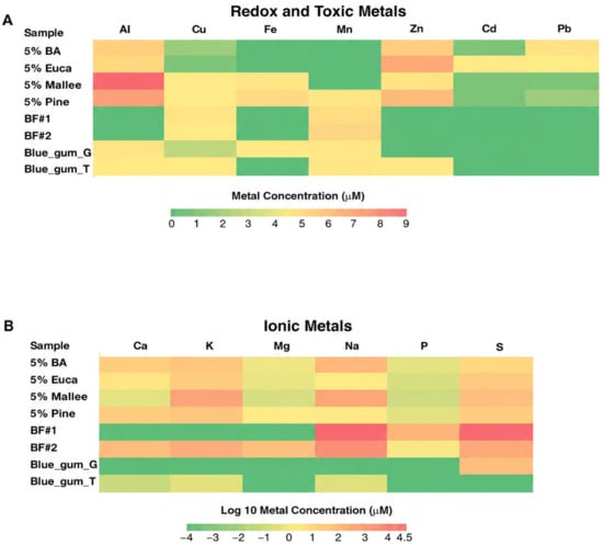
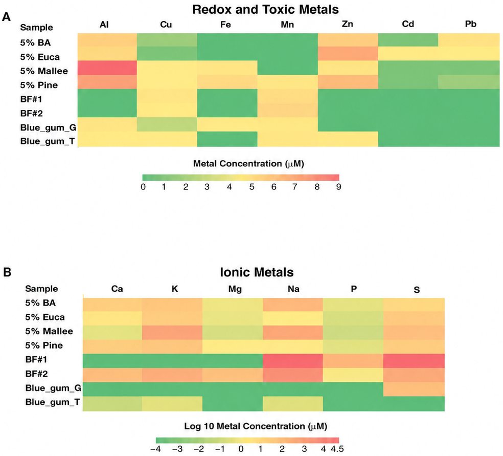
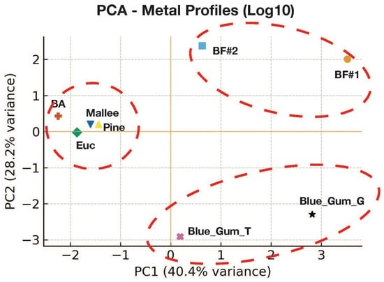
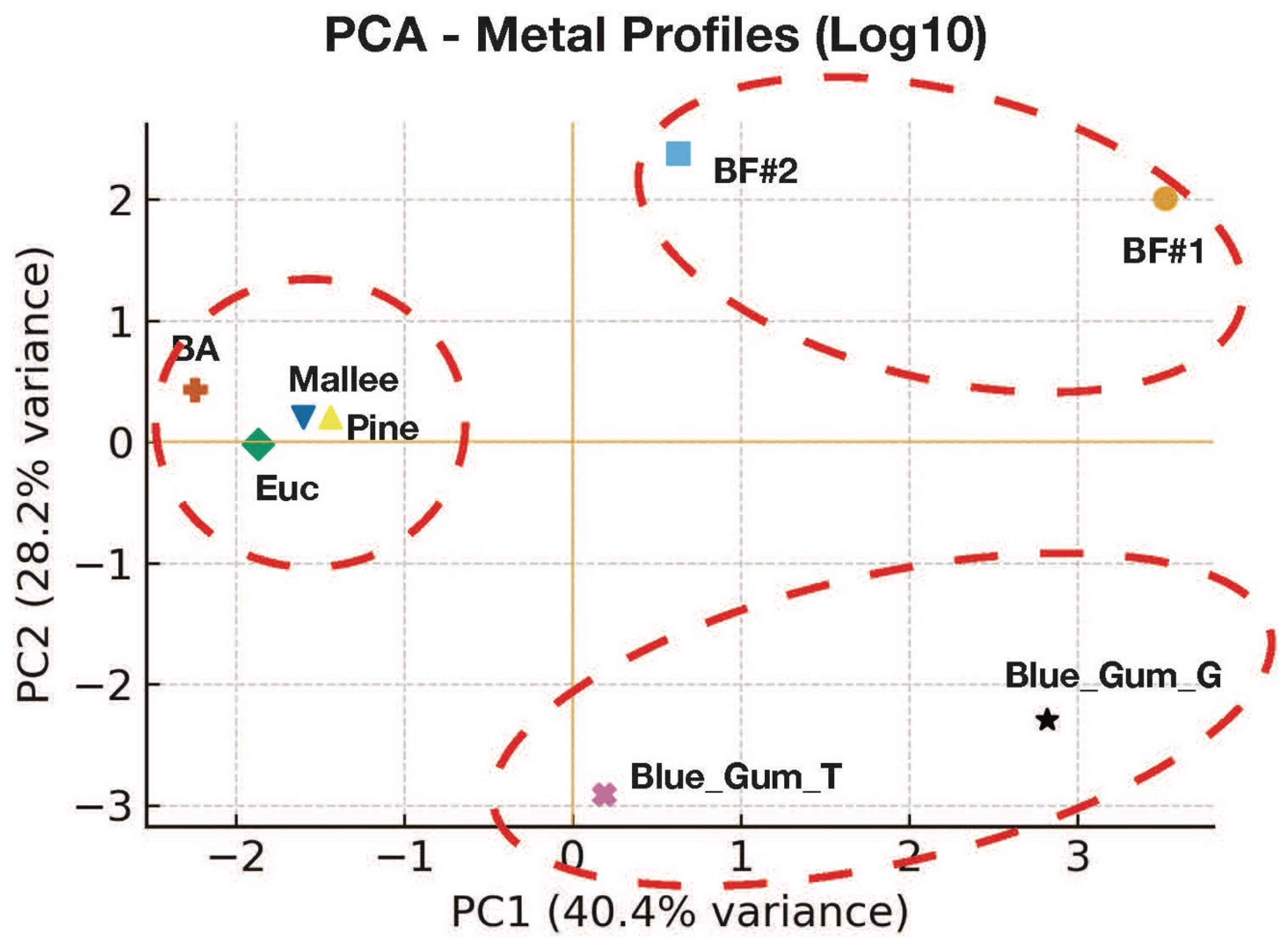

Disclaimer/Publisher’s Note: The statements, opinions and data contained in all publications are solely those of the individual author(s) and contributor(s) and not of MDPI and/or the editor(s). MDPI and/or the editor(s) disclaim responsibility for any injury to people or property resulting from any ideas, methods, instructions or products referred to in the content. |
© 2026 by the authors. Licensee MDPI, Basel, Switzerland. This article is an open access article distributed under the terms and conditions of the Creative Commons Attribution (CC BY) license.